1. Introduction
According to the statistics published by the United Nations Conference on Trade and Development (
https://unctadstat.unctad.org/wds/reportfolders/reportFolders.aspx, accessed on 30 January 2024), the 2022 merchant fleet worldwide adds up to about 2199 deadweight Mtons (102,889 ships), against 1418 Mtons in 2011 (83,283 ships). This increase in vessels and transported goods makes maritime traffic surveillance essential for different needs, such as border control, fisheries regulations, enforcement and monitoring of illegal activities, as well as for general security and emergency management [
1]. Following the annual reports of the European Maritime Security Agency (EMSA, [
2]), a growing tendency in the occurrence of maritime accidents becomes apparent; indeed, the number of incidents and casualties in 2011 (about 1300) more than doubled in 2016 (about 3300). The awareness about such a critical scenario fostered the scientific effort towards the development of novel solutions to counteract this worsening trend. At least for regions of particular interest, the integration of diverse tools and methods has been considered appropriate to build a robust maritime situation awareness system over an extended timeframe.
Whereas this is made possible by terrestrial or space-based identification systems, such as the Automatic Identification System (AIS,
https://www.imo.org/en/OurWork/Safety/Pages/AIS.aspx, accessed on 30 January 2024) and Long-Range Identification and Tracking (LRIT,
https://www.imo.org/en/OurWork/Safety/Pages/LRIT.aspx, accessed on 30 January 2024), in areas not covered by vessel traffic services, or when dealing with falsified or corrupted identification messages [
3], remote sensing remains the only means to achieve situational awareness by the maritime authorities. Satellite-borne Synthetic Aperture Radar (SAR) sensors are insensitive to weather and light conditions and capable of covering vast oceanic areas. This is why SAR is often a choice in the implementation of maritime surveillance systems.
Marine traffic understanding, however, is not only ship identification and tracking. Complete situational awareness must include specific tools to monitor the activities performed by ships at sea and to foresee their future behavior and potential effects. Aside from remote sensing, data science represents a valuable tool to enlarge the perspective attainable from individual observations or intermediate signal processing products to provide more complex assessments regarding maritime traffic status. This promising integration between field measurements and high-level data analysis is expected to represent significant beneficial progress regarding awareness of the operators and decisionmakers involved, thus ensuring valuable support for fast and proper actions.
In this paper, we first summarize the desired features of a marine traffic understanding system, with reference to the available literature; then, we present a real implementation developed within the framework of the European Space Agency (ESA) project OSIRIS Follow-On, which is the upgraded version of OSIRIS (Optical and SAR data and system integration for rush identification of ship models [
4]), a former ESA project ended in 2018.
Compared to the previous version, the implementation described herein introduces several innovations concerning (i) a new ship detection module modified to accept and process Thermal Infrared Imagery as additional input data, (ii) a revised ship classification module including a random forest classifier, whose performance has been assessed through a dedicated validation analysis, (iii) an additional procedure in the ship kinematics estimation module, in charge of estimating the speed of moving targets based on the analysis of SAR spectrum alterations, (iv) an SAR-AIS Data Fusion module in charge of matching the ship detection output with the collected AIS data through a properly defined similarity criterion, and, finally, (v) a ship route prediction module based on a supervised machine learning algorithm trained with a large-size ship reporting dataset.
In the following, the changes introduced are described in detail both for what concerns the theoretical innovation and the validation performed on selected experimental data. Also, a sequence of block diagrams, one for each module of the pipeline, has been produced as
Supplementary Material attached to this paper. Each diagram visually provides immediate insights about the main functionalities of the respective module in the pipeline.
This paper is organized as follows:
Section 2 briefly accounts for the state of the art concerning each module that usually forms a maritime monitoring platform pipeline.
Section 3 provides an overview of the platform, focusing on its salient features and functions.
Section 4,
Section 5,
Section 6,
Section 7 and
Section 8 report the novel solutions developed within each task of the pipeline, each accompanied by the respective experimental results.
Section 9 synthesizes outstanding aspects of the processing pipeline, either in terms of specific advantages or disadvantages. Conclusions are drawn in
Section 10.
2. Related Work
The maritime platform described in this paper operates through the integration of multiple functionalities that are sequentially applied to remote sensing data. The input imagery, captured by satellite-borne sensors within given time and space ranges, is injected into the system together with contextual AIS data obtained through independent dedicated sources (e.g., MarineTraffic,
https://www.marinetraffic.com, accessed on 30 January 2024, or equivalent providers). These images are processed through the cascade of multiple functional modules that constitute the platform core, each extracting the specific information of interest from the data. The entire set of outcomes is then conveyed to a WebGIS database, which is dedicated to data collection, management, and access.
Figure 1 provides a pictorial representation of the platform mode of operation, illustrating the chronological order of the processing pipeline and the main outcomes provided by each module.
The following sections report about the state of the art concerning each component of the proposed maritime traffic monitoring platform, with specific focus on the modules devoted to ship detection (SD), ship classification (SC), ship kinematics estimation (SKE), SAR-AIS Data Fusion (SADF), and ship route prediction (SRP).
2.1. Ship Detection
For many years, remote sensing tools and methods have been employed in maritime scenarios to ensure security and safety. Radar and SAR have been used for sea state monitoring, oil spill or ship detection, exploiting the capability of mapping large-scale areas, as well as the possibility to be operated with any weather and light (diurnal and nocturnal) conditions. In [
4], we present the module used in our platform to implement the task of ship detection based on SAR imagery, which feeds the related downstream modules. The detection technique used is based on a Constant False Alarm Rate (CFAR) approach. A sufficiently large area is then allowed around some target pixel, such that the largest possible ship can be entirely contained in it. This strategy is justified if we assume we are dealing with an open sea scenario where any two vessels are sufficiently far apart from each other. This algorithm, used on Sentinel-1 SAR imagery, is robust, reliable, and fairly fast. It produces high detection scores with a very low number of false negatives and positives. The algorithm was also parallelized to speed up the processing. In a general scenario, accurate instance segmentation could be necessary to distinguish any ship target from different objects, such as other ships, rocks, or harbor facilities [
5]. This is conducted, for example, in [
6] through a dedicated convolutional neural network. In our system, the task of finding a refined target footprint is assigned to the ship classification module. Some literature contributions propose a combined use of CFAR and deep learning algorithms (see, e.g., [
7,
8]). Those procedures are faster and more accurate, so they are worthwhile to be investigated.
Passive optical sensors in high-resolution panchromatic mode can serve the ship detection task, although they are mainly employed for ship identification purposes due to the excessive cost of commercial data and because the coverage area is small due to limited satellite swath at very high resolution. Further limitations are represented by meteorological and illumination factors that may strongly affect the signal quality (e.g., in the case of cloudy weather or nighttime conditions).
The thermal infrared band allows for several applications in remote sensing, such as monitoring urban heat islands and thermal plumes of warm water discharges caused by power plants and fire detection (see, for example, [
9,
10]). With respect to previous literature approaches, one of the novelties introduced in this work is represented by the usage of spaceborne thermal infrared (TIR) data for ship detection purposes. A few studies have previously been carried out using data acquired by TIR sensors mounted on ships and coasts in a local sensing configuration [
11,
12]. We propose the use of nocturnal TIR imagery for ship detection, taking advantage of the temperature difference between the main deck of ships and the surrounding seawater.
To the best of the authors’ knowledge, this is an unprecedented way to exploit this type of data. In
Section 4, the usability, benefits, and limitations of spaceborne TIR data for the implementation of a novel ship detection module are presented and discussed.
2.2. Ship Classification
In [
13], three basic approaches for ship identification from SAR imagery are recognized: (1) decision-based [
14], (2) pattern matching [
15], and (3) multi-channel classification [
16,
17,
18]. The features used for non-deep-learning classification, that is, the ones that are handcrafted to feed a specific classifier, can be divided into three classes: spatial (size and shape parameters), transformed (Fourier, Radon, Hough, etc.), and motion (course and velocity) [
19]. Aside from spatial (i.e., geometric) features, ship classification from SAR images can also rely on scattering measurements extracted from calibrated data. Indeed, different ship types can be characterized from both their geometry—size, aspect ratio, compactness, etc.—and the strength and distribution of the scattering centers in the ship structure. Of course, these possibilities depend strongly on the spatial resolution of the images at hand. The possibility of measuring geometric attributes in a reliable and repeatable way decreases as the resolution decreases; the same is true with scattering attributes. The spatial resolutions available, normally of meters or tens of meters in SAR images relevant to maritime applications, thus constitute a limitation for the grain of feasible classification and the related performance. As far as deep learning is concerned, it is proving to be increasingly effective in marine object recognition [
20,
21,
22], but the results produced from low-resolution data are not so overwhelmingly better than those obtained by algorithms based on handcrafted features [
23,
24,
25]. In [
26], it is proposed to improve the effectiveness of a convolutional neural network (CNN) classifier by leveraging handcrafted features in addition to the abstract features learned by the network. This hybrid approach deserves to be examined in depth as it provides solutions that avoid some common drawbacks of CNNs, such as the need for very large training sets associated with the number of learnable parameters in the network.
The possibilities provided by interferometry, Doppler processing, and polarimetry need high resolutions and image types that are not always available [
27,
28,
29,
30]. With moderate-resolution, single-channel images, many authors maintain that the only useful features are the geometric ones [
31,
32,
33]. As a high-resolution SAR image is obtained at the cost of a narrow swath, which is unsuitable for maritime surveillance, those authors also propose to work with moderate resolutions. Then, as the distribution of the strong scattering centers in moderate-resolution images does not have a clear pattern shown by high-resolution images, their discriminative power is reduced. This is partly confirmed by experiments (see
Section 5), even though the overall classification accuracy is improved anyway by using scattering features. Conversely, the geometric features are ‘relatively stable’. In our experience (see, e.g., [
4,
34]), we also noted that using strictly defined geometric features does not present any advantage over approximate geometric features with moderate resolutions. Thus, following [
32], we adopt the so-called “naive geometric features” (NGF) in our work with Sentinel 1 SAR images [
4,
35].
2.3. Ship Kinematics Estimation
The problem of estimating the speed of a moving vessel plays a key role in the processing pipeline of a maritime traffic surveillance system. Currently, a direct method to obtain the dynamic information of a vessel is based on the AIS. Alternatively, the vessel velocity information can be indirectly estimated by processing imagery captured by twin satellite constellations, such as TanDEM-X [
36]. Nevertheless, single SAR sensing missions can also serve the purpose, as illustrated in the following.
In general, SAR represents a powerful methodology to remotely survey and understand the heterogeneous properties of extended Earth regions. It captures punctual information related to individual scatterers, either concerning their scatterometric, geometric, or also kinematic properties. This is true for SAR products captured in different modalities, such as Single Look Complex (SLC) in StripMap (SM) mode or Interferometric Wide Swath (IW) in Ground Range Detected (GRDH) mode. Image processing techniques can be exploited to extract the velocity-related information intrinsically contained in the data and provide a reliable assessment of the target dynamics.
SAR imagery has been previously exploited for ship kinematics estimation purposes. In [
37], the kinematics estimation goal has been pursued by developing algorithms in charge of detecting, in IW GRDH input images, specific patterns relating to the ship velocity. For example, the wake pattern generated on the marine surface by the vessel passage carries information associated with the motion of the vessel itself. The plane waves directly observable on the boundaries of the wake cone (Kelvin wakes) feature a frequency value related to the target velocity magnitude. Thus, a spectral estimation procedure, e.g., based on the periodogram of the signal, enables the estimation of the plane wave frequency and accordingly of the velocity amplitude. Another approach exploits the visual representation of a moving target in SAR, which is affected by a fictitious displacement, called azimuth shift. The moving target in the image is represented in a location that deviates from the natural one, i.e., attached to the tip of the wake. The amplitude of this deviation increases with the radial component (along the range direction) of the target velocity; thus, its measurement represents a method to estimate the radial component of the velocity. Integrating with the outcome of auxiliary processing modules that also return the main orientation axis of the object (e.g., the ship segmentation procedure described in
Section 5.1), a complete estimation of the target velocity can be provided.
A number of considerations can be pointed out against each of the above mentioned methodologies. On average, the wake pattern in SAR imagery is very hard to capture due to the low intensity of the backscattered radiation. Moreover, the spatial extent of the Kelvin waves corresponds to a few pixels in the image, often too few to meet the Nyquist frequency constraint required for spectral estimation. Optical sensing also exhibits performance limitations since this type of sensor is operational only during daytime and can be affected by the presence of clouds. The awareness of these drawbacks and weaknesses motivated the request for a novel approach to the ship estimation task.
With respect to the mentioned literature approaches, the kinematics estimation problem in this work has been tackled from a different perspective. Indeed, it can be proven that the SLC SM SAR product retains velocity-related information in its phase value [
38] and, in particular, that the signal spectrum of a moving target is shifted with respect to the spectrum related to the neighboring water, assumed stationary. As will be further discussed in the following, the deviation between the centroids of these two spectra relates to the along-range target velocity, relative to the sea background. Following this direction, the ship kinematics estimation module presented in [
4,
39] has been further developed to include the novel approach. In
Section 6, the theoretical details of the implementation are described and results corresponding to the application of the software to a selected dataset are presented and discussed.
2.4. SAR-AIS Data Fusion
In recent years, there has been a growing interest in leveraging AIS data in conjunction with other technologies, such as SAR imaging, to improve situational awareness and enable more effective maritime surveillance, including vessel detection, tracking, and identification [
40,
41,
42].
AIS is a widely used technology in the maritime industry for ship tracking and collision avoidance. Its data provides time-based information about a ship’s ID, location, speed, heading, and other relevant parameters, which can be transmitted to other vessels, shore-based stations within range (74 km maximum), and satellites (S-AIS) [
43]. One of the main limitations of AIS data is that they are only available for vessels equipped with AIS transponders, which are not mandatory for all types of vessels and may be turned off for various reasons, including privacy concerns, malfunction, or illicit activities. Moreover, AIS data may not always provide accurate information about a ship’s identity as this information can be falsified or intentionally obscured by malicious actors. These limitations highlight the need for complementary technologies to overcome the gaps and inaccuracies and provide a more comprehensive view of maritime activity.
As said before, SAR images are first processed through dedicated ship detection methods to estimate the geographic coordinates of candidate targets. Then, the geographic positions of the targets are matched with the samples from AIS. SAR image metadata provide the timestamp of capture, which is used in conjunction with the SAR-derived positions to select a subset of AIS data. A time interval of several minutes before and after the SAR image acquisition is considered in order to find one or (preferably) two suitable AIS samples [
40]. In the next step, different techniques are usually employed to estimate the position of each AIS-identified ship at the time corresponding to the SAR image acquisition. If two samples are available, one after and one before, an interpolation is performed (usually linear, geodesic, or using a Hermite spline) [
42]. If only one sample is found, the ship position can be extrapolated instead, leveraging the velocity information to perform a Dead Reckoning (or an Inverse Dead Reckoning if the sample has been found only after the capture time) [
40]. The final step is to actually match the targets with the best possible estimated positions computed in the previous step, thus assigning each target to an AIS-identified ship (or mark the target as not found, and potentially non-cooperative, if no good match is found). Typical approaches employ a Nearest Neighbor (NN) algorithm, or a Global Nearest Neighbor (GNN) variant, such as the Hungarian algorithm [
42,
44], where the cost is defined as the Euclidean distance between the pair. It has been demonstrated that this matching phase can also be improved by relying on additional information that could be extracted from SAR images, such as ship category, size, heading, or velocity [
45].
2.5. Ship Route Prediction
A great deal of literature exists about SRP [
46,
47,
48]. Algorithms for SRP can be classified into three categories: (1) points-based, which predict only the immediately next position of the ship, (2) trajectory-based, which predict the whole trajectory, and (3) hybrid-based, which combine the previous two categories.
Points-based algorithms split the area to be monitored in different non-overlapping cells, all of which have the same size. Given the current status of a ship, they calculate the probability that each cell of the area will be occupied after a given period. This analysis is carried out based on historical data, generally extracted from AIS messages. This class of algorithms is implemented through different approaches, such as neural networks [
49,
50,
51], associative rules [
52], Kernel density estimation [
53], and K-NN [
54].
Trajectory-based algorithms exploit historical data to build clusters to extract and classify routes. Routes are then represented through a model, which can be improved through the inclusion of waypoints (harbors, offshore platforms, and entry and exit points in the area). Examples of trajectory-based algorithms exploit extended Kalman filter [
55], the similarity-based approach and kernel-based machine learning methods [
56], synthetic route knowledge [
57], a data-driven nonparametric Bayesian model based on a Gaussian process [
58], neural networks [
59], deep learning [
60], and generative models [
61].
In [
62], the authors describe an example of a hybrid-based approach called Traffic Route Extraction for Anomaly Detection (TREAD). TREAD uses the Density-Based Spatial Clustering of Applications with Noise (DBSCAN, [
63]) algorithm to cluster waypoints. Waypoints are then connected to form routes based on the AIS attributes of the ships (e.g., ship type). Once routes are built, predictions on ship routes can be performed. Given the current status of the ship (position, speed, and course), an ideal circular region is built around its position. All the routes included in this circular region are considered compatible with the ship. Finally, a compound probability is associated with each compatible route to determine the future trajectory.
Compared to the current literature, a focus on the specific area of Malta is considered, and an SRP module is implemented to work as a near-real-time application.
3. Platform Main Features
This section provides operational details about the proposed maritime traffic monitoring platform as a whole (illustrated in
Figure 1), such as the typologies of exploited data, the preliminary processing steps, and the interaction with the high-level interface.
Several data typologies have been considered as input data for the proposed platform. Among the available systems devoted to remote sensing purposes, the aforementioned SAR has been selected as a primary input source due to its capability to operate with any weather and illumination conditions. Suitable imaging resolution is ensured, as fine as 10 m in the case of ESA Sentinel IW GRDH. Even better accuracy is available if Spotlight imaging mode is chosen, providing a spatial resolution of a few meters for Cosmo Sky Med and TERRA Sar-X. Additionally, TIR sensors have also been considered and tested for the ship detection module. As described in the following, the usage of a thermal sensor enables implementing the detection task throughout the entire day, featuring a spatial resolution value around 100 m. Optical imagery may also be exploited for maritime monitoring purposes: high resolution and the additional color information enable implementing powerful recognition algorithms. The main drawback is represented by meteorological and illumination factors, which heavily affect this type of data. In this work, optical imagery has mainly been exploited to perform the manual matching between AIS data and satellite imagery in order to generate a ground truth for the SADF task. Also, in the experimental circumstances discussed in the following, AIS was exploited as a benchmark to assess the platform quality. In general, as described in
Section 7 and
Section 8, the AIS represented a ground truth source to test the accuracy of our procedures’ results. Finally, AIS also represented a source of data to build a training set and a test set to be exploited by the SRP learning algorithm, as discussed in
Section 8.
Since the region of interest (ROI) addressed in this work is located in the southern part of Sicily, including the Pelagie Archipelago, Pantelleria, and Malta, contextual AIS data have been accordingly collected. Actually, the collected data were not sufficiently numerous to provide training and test sets for the classification task; thus, the OpenSARShip (
https://opensar.sjtu.edu.cn, accessed on 30 January 2024) annotated dataset was employed as an additional data source for the ground truth generation (see
Section 5.2).
Before applying any platform algorithm, a preliminary discarding stage is applied to the data in order to detect and exclude land regions from the subsequent processing steps. This is carried out following the operations described in [
4].
An interested user will access the data processing services of the maritime platform through a dedicated WebGIS interface. Such a tool, a first prototype of which was formerly presented in [
4], supplies a wide range of functionalities, such as (i) have a quick look at real-time events, (ii) access historical information, and (iii) submit a request for monitoring a marine area of interest. Within this work, a novel implementation of the interface has been released, featuring a refinement in the input data retrieval process. In particular, given a new request from the user, the corresponding data are automatically downloaded by the system through the Copernicus Data Access Hub API. For this purpose, the interface download subsystem has been programmed to execute a series of API calls in order to check the availability of the requested imagery.
Ultimately, it is worth pointing out that one of the relevant goals of the proposed monitoring platform is to identify non-collaborative vessels. AIS transponder is indeed prone to malicious counterfeiting, potentially enabling a non-collaborative vessel to conceal any kind of illicit activity. Our system aims at providing a reliable tool to identify target ships that are not correctly monitored through the currently available systems and to extract from the data meaningful information that can be exploited to enrich the awareness of any concerned operator about the traffic status of an observed maritime area.
4. Ship Detection
As mentioned in
Section 2.1, in this upgraded version of our platform, the ship detection module based on SAR imagery has been complemented by an algorithm based on the acquisition and processing of TIR data. In particular, the proposed approach focuses on the detection of anomalies in the thermal infrared radiation emitted by anthropic targets at sea. In the first place, some effort has been devoted to the retrieval of TIR data, made available through reference public platforms (NASA and JAXA). This step was crucial to analyze the peculiarities of this type of data and to identify specific information about the physics of the sensors, information to be considered also during the operational implementation of the vessel detector. In the following, a CFAR implementation of a TIR anomaly detector is described and the related performance is discussed through quantitative metrics.
4.1. TIR Payloads Analysis
A comparison among a few relevant and publicly available TIR datasets (
https://database.eohandbook.com/esatpm/index.aspx, accessed on 30 January 2024) was performed. This data survey activity focused on the possible uses of spaceborne TIR imagery to support ship detection (both for diurnal and nocturnal satellite overpasses) and anthropic hot spots detection at sea (e.g., for emergency services), complementing SAR and Visible/Near Infrared optical sensors in maritime awareness systems. Specifically, data provided by Landsat (NASA-USGS), ALOS-2 (JAXA), and TERRA (NASA) missions have been considered and an analysis aiming at the identification of the relevant parameters that may affect the detector performance has been carried out.
The temperature of the main deck of a ship varies according to the sun radiation intensity throughout the day; hence, a first crucial parameter affecting the detection algorithm is the acquisition time, specifically the Local Time at Descending Node (LTDN) and the Local Time at Ascending Node (LTAN). In [
64], the entire-day trend of the temperature difference between the main deck of a ship and the surrounding water is described. From this analysis, it is clear that a ship thermal detector operating at daytime must be configured to identify hot radiating targets in the sensor field of view, while, in the opposite circumstance of night operation, it must be set up to search targets that are colder than the surrounding water background. In particular, it is observed that, during most of the daylight time, the deck temperature exceeds the surrounding water temperature (by an amount that depends on the sun position and the ship heading), while, after sunset, the deck temperature decreases due to nocturnal thermal radiation. As time passes by, and under the same environmental conditions (in terms of wind speed and temperature), the deck temperature value decreases more quickly compared to the surrounding water, and the absolute value of the deck–water temperature gradient increases. Hence, the optimal conditions to detect cold targets at nighttime occur before sunrise.
Another parameter affecting the detection is the Noise Equivalent Temperature Difference (NETD). This value indicates the minimum temperature difference resolvable by the TIR sensor. The NETD value can also be interpreted as a property of the ship detector sensitivity: the lower the noise (and thus the NETD value) of the detector, the smaller the temperature differences that can be detected by the infrared camera.
A third parameter affecting the CFAR-based detector performance is the geometric resolution, namely the Ground Sampling Distance (GSD) or the Ground-Resolved Distance (GRD), representing, respectively, the pixel resolution of the TIR camera and the minimum distance between two resolvable points on the ground.
Finally, the accuracy of the temperature measurement deserves some consideration. It does not affect the detection capability of the CFAR algorithm, which is based on temperature variations, but it directly affects the Land Surface Temperature (LST) and the Sea Surface Temperature (SST) maps production. Additionally, for the purposes of improving the measurement of the actual temperature, atmospheric correction by using a certified radiometric transfer model and ancillary meteorological data is desirable.
Table 1 reports a summary of several TIR satellite sensing campaigns, with quantitative specification of the parameters identified as relevant for the detection purpose. To this aim, the satellite/payload combination providing the best fitting features is the ALOS-2/CIRC mission.
4.2. Target Detection Results
An already available CFAR-based detector (see
Section 2.1) has been adapted for the new purpose and calibrated to extract thermal anomalies inside TIR images. The algorithm detects the image cells with temperature values that meaningfully deviate from the surrounding ones. Concerning the ship detection module, it is worth remarking that the detector is robust against the presence of near-shore targets. This is obtained thanks to a pre-processing stage that, exploiting the openstreetmap dataset (
https://www.openstreetmap.org/, accessed on 30 Janaury 2024), produces a 100 m buffer zone around the shoreline that enables removing land and fixing georeferencing errors.
Two types of images were elaborated: the native panchromatic TIR and the elaborated panchromatic Brightness Temperature. The latter provides a relative measurement of the temperature; in particular, the pixel amplitude value does not refer to the temperature value at sea altitude but represents instead the radiometric value measured by the sensor at the top of the atmosphere (ToA).
Table 2 and
Table 3 report the analysis of the ship detection results obtained by processing two TIR images, captured by Landsat-8.
The evaluation metrics were calculated by visual inspection of the Blue–Green–Red image in the first case and of the B10 ToA radiometry image (i.e., the ToA radiance measured by the Landsat-8 TIR sensor in the 10.6–11.19
m band) in the second case. Note that
Table 3 shows zero false negatives; in fact, many targets could possibly be missed by a simple visual inspection, and no ground truth is available in the absence of AIS data.
5. Ship Classification
5.1. Feature Extraction
The ship detection module provides rectangular image chips extracted from the SAR scene, each containing one of the detected targets. When processing one of those images, a segmentation algorithm needs to extract the, at least approximate, location and shape of the target to be classified. This can be obtained easily by binarizing the image with a suitable threshold, eliminating the spots that are too small to represent a ship, and merging the connected components that are very close to each other to represent potentially different parts of the same ship. The gross target footprint thus obtained then needs to be refined in order to enable the relevant features to be extracted. Indeed, any classification technique not based on deep learning needs first to select the features that are potentially useful to discriminate between the different ship types to be identified. Our refinement approach starts by determining the principal inertia axes of the input footprint to evaluate the ship size and heading. The heading information and the refined target location are not used for classification but passed to the kinematics module (see
Section 6). The subsequent strategy to refine the footprint is partly described in [
4] and the references therein. A further refinement follows [
65]. The result is a connected domain with its minimum enclosing rectangle, from which the target length, breadth, and other shape characteristics can be evaluated.
As mentioned in
Section 2.2, we use the NGF features proposed in [
32] and reported at the first eight positions in
Table 4. All of them only derive from the length overall and the breadth overall of the ship. For the strict geometric definitions, also depending on the shape of the footprint, see [
32]. Moreover, we need to know whether some scattering features are also useful to reduce the classification error, contrary to [
31,
32,
33], where these features were ignored, with the motivations mentioned in
Section 2.2. The features chosen, reported at positions 9–16 in
Table 4, can be computed, as described in [
34], from the calibrated SAR image cropped to the refined footprint; see
Figure 2 for an example.
The peaks referred to in the table are derived from the longitudinal scattering profile, also reported in the figure, obtained by averaging the scattering intensity within the refined footprint along lines orthogonal to the ship keel. The mean values at positions 9 and 14–16 in
Table 4 are evaluated, respectively, by averaging the intensities over the whole footprint and its stern, midship, and bow sections, highlighted in the figure and delimited by the stern abscissa, the bow abscissa, and the profile relative minima closest to one third and two thirds of the length overall. Since the most common location of the maximum scattering in ships is at the stern, in our implementation, the “stern” is always assumed to coincide with the highest between the first and the last peak in the scattering profile.
5.2. Classification
The ship classification module was conceived as a machine learning algorithm assisted by a “ground truth” database, populated by feature sets derived from reliably identified targets; see [
4]. This database was designed to establish links between possibly multiple feature sets and any single identified ship. Its structure is thus split into two parts. The so-called “static part” features a single record per each unique ship, containing its name, type, and other administrative and dimensional information, such as the Maritime Mobile Service Identity (MMSI), the length, and the breadth overall. A record in the static part may not be related to any extracted SAR feature set since the relevant information is derived from some maritime database or official ship register. Conversely, the “dynamic part” of the database contains all the feature sets that have been reliably associated with an identified ship. Of course, during the system operation, several feature sets can be associated with the same ship. A dedicated table in the database is devoted to establishing the links between features and ships at any time when a target identification is reliably validated by an accredited supervisor. By this mechanism, the ground truth database can be updated during the normal system operation. It can be used to either cluster the feature sets and infer the most likely type associated with the current input or periodically retrain a classification algorithm and keep it updated with the current ground truth.
This second option has been pursued in the current implementation of the classification module, where a random forest strategy [
66] has been designated as the classifier and tested using the annotated OpenSARShip dataset [
67] to form both the training and the test sets. The ground truth database was populated by the static data extracted from about 2700 records in OpenSARShip and by the “dynamic” features computed from the related Sentinel 1 image chips in VV and VH polarizations, representing four ship types: bulk carriers, cargo ships, container ships, and tankers. Some of these data were used to train a number of random forest classifiers, each with a different feature set, and the remaining data were used to form never-seen-before test sets with numbers of ships per type as balanced as possible. For the time being, the polarization has not been included among the features, and the classification has been performed separately for the VV and VH cases. The best overall accuracy [
34], within a 95% confidence interval [0.58, 0.69], was obtained from VH images using 11 features:
,
P,
L,
A,
,
,
W,
,
,
, and
(sorted by decreasing importance, computed as the mean decrease in the Gini impurity after replacing each feature with a random value [
68]). The corresponding confusion matrix, obtained with a test set including 100 bulk carriers, 100 cargo ships, 64 container ships, and 22 tankers, is reported in
Table 5. The results from all the experiments are reported in
Figure 3 in terms of estimated accuracies and 95% confidence intervals for feature subsets with increasing cardinality. The test set used is the same in all the experiments, so the no-information rate (NIR) is constant: 0.35 in all cases. As seen above, the feature set reaching the best accuracy contains five scattering features, thus demonstrating their positive effect even with moderate resolutions. Indeed, the best accuracies obtained from the geometric features alone are always much lower than the ones obtained with both kinds of features. Note, however, that the features that characterize the spatial distribution of the peaks in the scattering profile (
,
, and
) are not included in the feature set obtaining the best accuracy.
6. Ship Kinematics Estimation
Given a point-like stationary scatterer, the series of frequency values of the SAR backscatterings (the Doppler history) depends on the relative distance between target and sensor, and it is possible to prove (see [
38] for details) that the frequency has a linear dependency on the time variable and thus that the related power spectrum has an approximately rectangular shape (linear chirp-like), centered on the zero frequency value. In the case of a target with non-null along-range velocity component, the spectrum of the corresponding signal deviates from the center symmetry as a consequence of the additional Doppler effect. The deviation
depends on the along-range velocity component
:
where
is the radar center wavelength,
is the corresponding frequency value, and
c is the speed of light.
According to this, the velocity estimation algorithm has been implemented based on the following sequence of operations: (i) estimate the spectrum of a signal portion including the candidate target alone, (ii) repeat the spectral estimation operation on a stationary reference region, i.e., with no target displayed, and, finally, (iii) compute and compare the frequency centroids of the estimated spectra. If the target heading is known or estimated, e.g., returned by the ship classification module presented in
Section 5, the entire velocity vector can be eventually obtained.
The estimation of the spectrum of the azimuth signal is performed by extracting, at fixed range, a sequence of complex signal samples along the azimuth direction (see
Figure 4) and computing the corresponding power spectrum. Since a target’s SAR footprint typically spans more than a single range value, multiple spectral estimations can be computed for one target. A single final estimate is eventually obtained by averaging the multiple estimated spectra.
The proposed method has been validated on a small dataset, assembled starting from two Sentinel 1 A SLC SM scenes (scenes downloaded through
https://scihub.copernicus.eu/, accessed on 30 January; Id scene 1:
{S1A_S2_GRDH__1SDV_2016072 7T060537_20160727T060606_012330_01331F_14B3, S1A_S2_SLC__1SDV_20160727T060537_ 20160727T060606_012330_01331F_3D33}; Id scene 2:
{S1A_S1_GRDH_1SDH_20160609T060 543_20160609T060611_011630_011C9B_E709, S1A_S1_SLC__1SDH_20160609T060543_20160 609T060611_011630_011C9B_3DD0}), captured off the Dutch coast, in front of the North Sea. For every moving vessel identified in each map, a small image has been generated, cut out from the original one, in order to include the vessel only. A total of 15 targets have been detected and exploited to assemble the dataset. Every target has been processed to estimate the radial component of the velocity, first adopting the azimuth-shift-based method and employing the estimated value
as ground truth reference, then adopting the Doppler-centroid-based method, which returned the corresponding estimate
. The results are compared in
Table 6 and through the scatterplot in
Figure 5.
To assess the method accuracy, a few statistical quantities have been computed, namely the maximum observed deviation, the root mean square deviation, and the correlation coefficient. The resulting values obtained employing the entire dataset are reported in the first row of
Table 7. A few elements (number 2, 4, 5, and 13 in
Table 6, red marked dots in
Figure 5) exhibit a discrepancy in the estimated velocity values. A possible reason for these observed anomalies may relate to the lack of a sufficient number of pixels employed for the spectrum estimation. As known, the resolution of the discrete Fourier transform depends on the number of signal samples (i.e., the length of the azimuth SAR sequence), which indirectly affects the accuracy in the measurement of the centroids deviation. For the identified anomalies, too few pixels were available, causing the output results to deviate from the expected ground truth values (i.e., the azimuth shift measurements). As reported in the second row of
Table 7, the performance improves if the strongest outliers are excluded from the test dataset.
7. SAR-AIS Data Fusion
The SAR-AIS Data Fusion module integrates SAR and AIS data for ship detection and identification by applying the state-of-the-art approaches discussed in
Section 2.4. It takes as input a set of vectors representing the coordinates of the ships (targets) as identified from SAR imagery by the SD module, and a series of AIS data corresponding to the area and time interval of interest related to the image. The matching algorithm provides, for each vector, zero or one matching vessel MMSI derived from AIS data, as well as a confidence score for each match. Positions are always handled by converting them to n-vectors [
69], i.e., 3D vectors normal to the Earth ellipsoid. This ensures reliability of the module’s computations at any geographic location, minimizing errors associated with different coordinate systems and projections, as well as avoiding complex handling of corner cases (e.g., projection discontinuities, poles, or crossing of the international date line). Similarly, the module addresses possible ambiguities regarding time (e.g., other modules using different formats for dates, ships entering a different time zone, or switching to daylight saving time) by adopting a mandatory timezone-aware approach, enhancing data consistency.
The matching module performs several steps to identify matches between SAR image targets and AIS vessel positions. First, it conducts a spatio-temporal query to the database of AIS historical data to extract ships having samples comprised within the spatial and temporal coverage of each target ship detected in the SAR image. Then, it queries the AIS database to search for two samples relative to each of the extracted ships, one before and one after the SAR image acquisition time. Next, it converts the obtained coordinates to n-vectors in order to perform a geodesic interpolation to estimate the ship’s position at the central time of the SAR image acquisition interval (see
Figure 6).
The module then uses geodesic distance-based scoring to rank the candidate matches based on their estimated proximity to the position of the corresponding target ship in the SAR image, discarding possible matches that would be over a specified threshold distance. All the obtained target–candidate–score tuples are then added to a global list of possible matches. The best matches are then extracted from the global list on a first-come-first-served basis.
Ideally, the data fusion module has been designed to also take as input the speed and ship type values estimated by the SKE and SC modules. As a matter of fact, we ascertained that, in the collected dataset, the reported speed and ship type values were not reliable (this is not uncommon, as also stated in [
45]), so better results were achieved by neglecting those additional inputs.
Evaluation
In order to perform an evaluation of the SAR-AIS Data Fusion module, we created a ground truth dataset (GT) from two SAR images and three optical images with corresponding AIS data (both T-AIS and S-AIS). The chosen area of interest (AoI) is the sea east of Malta, including both near-shore and open sea traffic. A total of 299 targets found in the images have been manually annotated by experts. The images and AIS samples have been inspected on GIS software (Qgis 3.16) and for each target the corresponding MMSI was indicated, if present. A null value indicated that the expert was not able to find any match.
The module was provided as input the same targets and AIS data provided to experts, and the output results were compared with the ground truth (see
Figure 7). The confidence score distribution was analyzed to identify a suitable threshold for distinguishing between reliable and unreliable matches. A small number of false positives were still present at higher confidence scores. This observation suggests that choosing larger threshold values may be suitable to further reduce the occurrence of false alarms.
The final evaluation has been conducted by organizing the results in a confusion matrix with values defined as follows: true positive (TP): module and GT assigned the same MMSI to a given target; true negative (TN): module and GT did not assign an MMSI to a given target; false positive (FP): module assigned an MMSI to a given target, but the GT assigned none; false negative (FN): module did not assign an MMSI to a given target, and the GT assigned one; mismatch (MM): module and GT assigned different MMSIs to a given target.
The resulting overall accuracy is 85.95%. See
Figure 8 for details.
8. Ship Route Prediction
The SRP problem can be solved with the differentiation of an AoI into cells followed by the identification of the cell that will be occupied by a ship after some time. This is a multiclass classification problem where every target class corresponds to a cell of the grid identified by a row and a column. As input features, we consider the current status of the ship, which includes its current latitude, longitude, speed over ground, course over ground, and class. As an additional feature, we could consider a date time variable. However, we proved in [
70] that the use of the date time feature does not improve the performance of the SRP algorithm in a practical scenario.
In a previous work [
71], we developed a comparison among different multiclass classification algorithms to solve the SRP problem. Here, we focus the analysis on the K-Nearest Neighbors classifier and retrain it with new data. The adopted approach can be described as the sequence of two steps, i.e., data preparation followed by model training and evaluation.
8.1. Data Preparation
The dataset used to train the two algorithms was built from 188,130,529 AIS messages extracted from Astra Paging, covering a time interval from 26 December 2015 to 24 December 2017 and referring to the AoI near Malta. We considered a cell size of squared degrees.
To prepare the data for model training and evaluation, we created a new dataset, actually a subset of the original one, properly cleaned and balanced. We applied the following preprocessing techniques to the raw dataset: (a) cleaning, (b) discretization, (c) normalization, and (d) balancing.
Data cleaning consisted, in this case, of the deletion of all the records, which did not satisfy the following criteria: speed smaller than or greater than , course greater than 360°, and records where the MMSI was present only once.
Data discretization represented the transformation of values from a continuous domain to a discrete one. We discretized the course over ground, the speed, the latitude, and the longitude. To obtain the discretization of the course over ground, we divided the course into eight clock faces, as illustrated in
Table 8.
Speed was discretized by adopting four slots, as shown in
Table 9. Finally, latitude and longitude were discretized by setting the latitude to the value of the row in the matrix representing the AoI and the longitude to the column in the same matrix.
Data normalization involved adjusting values measured on different scales to a common scale. In this work, we applied single-feature scaling to each input feature.
Finally, data balancing involved setting the number of samples for each target class to a fixed value, in this case . To this aim, the following approach was adopted: (1) undersample the classes with more than records through random undersampling; (2) undersample the classes with a number of records between and through cluster centroids; and (3) oversample the classes with less than records through random oversampling. At the end of the data preparation phase, 2397 classes remained, each representing a different cell of the AoI.
8.2. Model Training and Evaluation
After the data preparation stage, the resulting dataset contained 2,397,000 records with 2397 classes. We performed model training through grid search with K-fold cross-validation, with k = 5. The training set contains 2,157,300 records and the test set the remaining records. To evaluate the model’s performance, we compared it with a baseline model, which generates randomly uniform predictions from the list of unique classes.
Table 10 compares the two models regarding precision, recall, and accuracy.
The baseline model has very poor performance due to the high number of classes (2397). The explanation is quite intuitive. The probability that the ship will be in a cell at some point is 1/number of classes, i.e., 1/2397 = approximately 0.0004. This value more or less corresponds to the metrics in the case of the baseline model. This situation occurs because the baseline model does not consider the previous position of the ship. Our model, instead, considers the ship’s previous position, which provides a notable reduction in the number of cells potentially occupied at the next position of the ship. A further improvement in the SRP system could be developing a mathematical model considering the ship’s motion. We postpone comparing this mathematical model and our model for future work.
8.3. SRP Results
To test the performance of the algorithms in a real case, we set up a practical experiment. We extracted the satellite image used in this experiment from the Copernicus Open Access Hub (
https://scihub.copernicus.eu/, accessed on 30 January). In detail, we looked for a satellite image that referred to a date also contained in our AIS dataset to check the correctness of the results. The extracted image is related to an area south of Sicily and refers to the date 25 May 2017, 16:55:56 (the image is S1A_IW_GRDH_1SDV_20170525T165531_20170 525T165556_016741_01BCE3_614D.SAFE). Through the various modules of the OSIRIS project, we extracted the ship’s position, speed, direction, and class. The ship detection module detected about 100 ships in the image. Then, we included the results of the previous modules as input to the SRP module to predict the position after one hour.
Through the data fusion module, we built mapping between the AIS data and the ships extracted from the image. This permitted us to reconstruct the correct path of the ship and verify the correctness of the predicted values by SRP.
Figure 9 shows the predicted cells for ships with corresponding ID 100. The initial position is identified by a black dot, with a direction going towards the top left part of the figure. The dotted line (in orange) shows the path of the ship identified by the data fusion model according to AIS data. The red dot shows the ship’s signaled position after an hour. The four rectangles represent the next positions in terms of cells predicted by the SRP module after an hour. The darker the cell color, the higher the probability that the cell will be occupied by the ship after an hour. As we can see from the figure, our model perfectly predicts the most probable cell after one hour.
9. Discussion
This paper describes a system for maritime situation awareness based on remote-sensed data, possibly helped by fusing them with AIS information. It is structured as a pipeline of independent modules working asynchronously, only bound to comply with specific data exchange protocols. If these protocols are maintained, each software module can be amended or replaced with no harm for the other modules and no need to alter the system backbone. Also, since the data exchange is based on a unique file system, located anywhere, there is no need to host all the modules in the same machine. Conversely, it could be necessary to change or enrich the data exchange protocol in the case where some system functionalities are to be extended. This could entail either adding new input or output variables to the existing modules, with the need to change the content of some exchange files, or add new modules, with the consequent need to alter the backbone structure and produce new data exchange files. Even the current prototypical system implementation is quite fast in producing all its outputs, taking typically less than an hour to process a scene with a few hundred targets.
This implementation does not include a supervisor process. Any error in a module, even if detected, does not help the downstream system to cope with the lack of some parameter. If the downstream modules are able to usefully process the available data, then just some global output information will be missing; otherwise, all the information regarding the affected target will be lost. We could attempt to overcome this limitation, indeed, by adding a suitable supervisor module and possibly some feedback between downstream and upstream modules. Before designing a generally usable system, we should improve the reliability of all the modules and optimize their operation.
Specifically, this includes:
Concerning the ship detection module, possible false positives may emerge in nocturnal imagery due to pixels with abnormal low brightness amplitudes, a condition that could take place, e.g., in the presence of clouds. On the other hand, false negatives can also be generated by weakly radiating targets (e.g., in the case of small targets or in case the backscattered data are captured when hot winds hit the main deck). Under these conditions, the detection procedure generates missed targets because the ship and the surrounding sea temperatures are almost the same. Intrinsic physical limitations of the TIR detector and lens (low spatial resolution, low detector sensitivity, NETD, and reduced lens diameter) entail that such targets cannot be detected. New generations of TIR detectors, with the highest performance, are required.
The new functionality of classification from SAR images provides accuracies of less than 70% through the entire test set. The problems to be solved to improve this result include increasing the granularity of the classification by enabling the module to include more ship types and increasing the classification accuracy, thus making the results more reliable and useful in practice. These two requirements are somewhat contradictory since the classification accuracy normally decreases with an increasing number of classes, even though it is maintained well above the NIR.
As mentioned in
Section 6, the performance of the kinematics algorithm based on the Doppler history in SAR images is heavily affected by the number of pixels exploited for spectrum estimation. Indeed, the accuracy of the spectral centroid estimate is inversely proportional to the length of the azimuth sample sequence. As a consequence, the module performs badly with targets occupying too few resolution cells. It is worth remarking that the outliers identified in the module validation correspond to those with the smallest number of target-related pixels and that their exclusion from the dataset boosts the estimation performance. A second factor of concern is represented by the presence in the region of interest of secondary scatterers (additional vessels and portions of secondary targets wakes), i.e., objects whose reflection magnitude is comparable with that of the primary target. This may affect the accuracy and the reliability of the spectral estimation since the spurious reflectors may have statistical properties that differ from those of the background clutter. Finally, the signal coming from the primary target must reflect a sufficient portion of the incident radiation, possibly some orders of magnitude above the surrounding clutter, in order to have relevant weight in the spectral estimation procedure.
The SADF module has a significant limitation when AIS data are insufficient, causing issues with sample retrieval and interpolation, leading to false negatives. On the other hand, in an overly congested area, there is an increased risk of mismatches. The threshold to distinguish between reliable and unreliable matches may vary accordingly.
The validation experiments concerning the SRP module confirmed that estimating the ship’s trajectory is a hard task to accomplish. Despite the limited number of experimental samples employed for validation purposes, the achieved results are encouraging since they show that the described methodology is correct.
10. Conclusions
The maritime surveillance pipeline presented here is able to display the traffic situation in a large area with a relatively low elapsed time from the ingestion of the remote-sensed data. The current version has been tested extensively and presents several improvements over the one presented in [
4]. The residual limitations and drawbacks discussed above can be overcome by either improving the algorithms or extending the system functionalities by adding new computational models. By virtue of the system structure, both tasks are feasible with minimal or no intervention regarding the pipeline protocols. However, the mentioned opportunity to introduce a supervisor process and/or suitable feedback loops between modules could require a complete rethinking of the entire system. This is one of the aspects that will be dealt with in the future. The individual modules will also be analyzed to correct possible malfunctions and optimize their performance.
The TIR data processing capabilities can help in reducing the number of undetected targets, especially with small-target vessels, but also present difficulties. Acquiring a larger TIR database can make the ship detection module more robust against threshold errors, thus increasing the recall of targets that are small or characterized by low temperature contrasts with respect to the sea surface. Moreover, since clouds appear as cold objects in the TIR images, searching a ship as a cold spot during nocturnal overpasses has a twofold limitation: the clouds can hide the targets and also generate noise. On the other hand, the area generally covered by clouds is often larger than the largest ships, so a size-based filter could partially mitigate these effects. The influence of the sensor performance in terms of spatial resolution (GRD/GSD) and radiometric performance (resolution, accuracy, and precision) on detection accuracy has to be investigated. A massive data fusion between AIS data and TIR imagery will enable the creation of significant statistics, on whose basis the performances of the available orbiting TIR sensors can be analyzed and compared.
As far as classification is concerned, further studies on deep learning methods could solve the problems mentioned in
Section 9 if the methods developed are able to extract meaningful features when trained on small sets of moderate-resolution images. This would also avoid the need of identifying and selecting the most significant handcrafted features. Recently, several deep learning proposals have been presented in the literature (e.g., [
21,
26]) that could overcome the existing difficulties.
As far as the velocity computation task is concerned, it is worth emphasizing that the presented approach is built on the detection of spectral alterations in the SAR azimuth signal and, in particular, on the measurement of the spectrum centroid deviations, currently tested on ESA Sentinel images with medium resolution (≳10 m). The accuracy of the centroid estimation process depends on the sampling resolution in the discrete frequency domain; hence, the acquisition of SAR imagery featuring finer resolutions (COSMO-SkyMed 2nd Generation, TERRA SAR X) could enhance the estimation performance. A potential solution to the lack of experimental data for validation purposes may be represented by methods, proposed in recent years (e.g., [
72]), for the artificial generation of data. Such methods are mainly based on the usage of deep neural network architectures. Future work will be devoted to the assessment of the potentialities expressed by advanced machine learning tools, also as a means to tackle data scarcity issues.
The matching algorithm implemented for the data fusion proved effective in correlating SAR-detected targets and AIS vessel positions. Further improvements will focus on the analysis of areas exposed to heavy traffic, implementing refinements in the selection of the threshold exploited to distinguish between reliable and unreliable matches. An expected hindrance for future developments is represented by the lack of data for testing purposes. For this reason, the expansion of the ground truth dataset, an operation currently performed by hand, will represent the main and most time-consuming task to be developed.
Future work will be devoted to an in-depth analysis of alternative methods, such as those based on deep learning or large language models.
Author Contributions
M.R. (Marco Reggiannini) realized and tested the kinematics module, conceived the structure of the paper, and led the writing. C.D.P. and C.M. conceived the overall system structure, realized and tested the ship detection module, and, in collaboration with all the authors, defined the data exchange procedures in the OSIRIS system. M.M. and M.T. conceived and realized the ground truth database in the SC module and its integration with the overall system. M.R. (Marco Righi) and E.S. realized and tested the classification algorithm. A.L.D., C.B., A.D. and A.M. (Andrea Marchetti) realized and tested the data fusion and the ship route prediction modules. A.M. (Antonino Mistretta) realized and tested the WebGIS interfaces. C.D.P. coordinated the entire project. All authors have read and agreed to the published version of the manuscript.
Funding
Partial support was provided by ESA General Support Technology funding Programme, RFQ/ITT no. ESA-IPL-POE-SBo-sp-RFP-1008-2015.
Data Availability Statement
Data are contained within the article.
Acknowledgments
The authors would like to thank Michela Corvino (ESA) for useful discussions and suggestions.
Conflicts of Interest
Claudio Di Paola and Costanzo Mercurio were employed by the company Mapsat S.R.L. Antonino Mistretta was employed by the company SisTer S.R.L. The remaining authors declare that the research was conducted in the absence of any commercial or financial relationships that could be construed as a potential conflict of interest.
References
- Heiselberg, H.; Stateczny, A. Remote Sensing in Vessel Detection and Navigation. Sensors 2020, 20, 5841. [Google Scholar] [CrossRef] [PubMed]
- European Maritime Safety Agency. Annual Overview of Marine Casualties and Incidents 2022. 2022. Available online: https://emsa.europa.eu/csn-menu/items.html?cid=14&id=4867 (accessed on 3 February 2022).
- Iphar, C.; Napoli, A.; Ray, C. Detection of false AIS messages for the improvement of maritime situational awareness. In Proceedings of the OCEANS 2015-MTS/IEEE Washington, Washington, DC, USA, 7–12 June 2015; pp. 1–7. [Google Scholar] [CrossRef]
- Reggiannini, M.; Righi, M.; Tampucci, M.; Lo Duca, A.; Bacciu, C.; Bedini, L.; D’Errico, A.; Di Paola, C.; Marchetti, A.; Martinelli, M.; et al. Remote sensing for Maritime Prompt Monitoring. J. Mar. Sci. Eng. 2019, 7, 202. [Google Scholar] [CrossRef]
- Ke, X.; Zhang, T.; Shao, Z. Scale-aware dimension-wise attention network for small ship instance segmentation in synthetic aperture radar images. J. Appl. Remote Sens. 2023, 17, 046504. [Google Scholar] [CrossRef]
- Chen, P.; Zhou, H.; Li, Y.; Liu, B. A Novel Deep Learning Network with Deformable Convolution and Attention Mechanisms for Complex Scenes Ship Detection in SAR Images. Remote Sens. 2023, 15, 2589. [Google Scholar] [CrossRef]
- Yasir, M.; Wan, J.; Xu, M.; Sheng, H.; Zhe, Z.; Liu, S.; Colak, A.T.I.; Hossain, M.S. Ship detection based on deep learning using SAR imagery: A systematic literature review. Soft Comput. 2022, 27, 63–84. [Google Scholar] [CrossRef]
- Cao, H.; Duan, Y.; Li, J.; Wang, R.; Zhao, Y. Study on the Combined Application of CFAR and Deep Learning in Ship Detection. J. Indian Soc. Remote Sens. 2018, 46, 1413–1421. [Google Scholar] [CrossRef]
- Karyati, N.E.; Sholihah, R.I.; Panuju, D.R.; Trisasongko, B.H.; Nadalia, D.; Iman, L.O.S. Application of Landsat-8 OLI/TIRS to assess the Urban Heat Island (UHI). IOP Conf. Ser. Earth Environ. Sci. 2022, 1109, 012069. [Google Scholar] [CrossRef]
- Sobrino, J.A.; Del Frate, F.; Drusch, M.; Jiménez-Muñoz, J.C.; Manunta, P.; Regan, A. Review of Thermal Infrared Applications and Requirements for Future High-Resolution Sensors. IEEE Trans. Geosci. Remote Sens. 2016, 54, 2963. [Google Scholar] [CrossRef]
- Zhang, M.M.; Choi, J.; Daniilidis, K.; Wolf, M.T.; Kanan, C. VAIS: A dataset for recognizing maritime imagery in the visible and infrared spectrums. In Proceedings of the 2015 IEEE Conference on Computer Vision and Pattern Recognition Workshops (CVPRW), Boston, MA, USA, 7–12 June 2015; pp. 10–16. [Google Scholar] [CrossRef]
- Li, Y.; Li, Z.; Zhu, Y.; Li, B.; Xiong, W.; Huang, Y. Thermal Infrared Small Ship Detection in Sea Clutter Based on Morphological Reconstruction and Multi-Feature Analysis. Appl. Sci. 2019, 9, 3786. [Google Scholar] [CrossRef]
- Ouchi, K. Recent Trend and Advance of Synthetic Aperture Radar with Selected Topics. Remote Sens. 2014, 5, 716–807. [Google Scholar] [CrossRef]
- Margarit, G.; Tabasco, A. Ship classification in single-Pol SAR images based on fuzzy logic. IEEE Trans. Geosci. Remote Sens. 2011, 49, 3129–3138. [Google Scholar] [CrossRef]
- Gibbins, D.; Gray, D.A. Classifying Ships Using Low Resolution Maritime Radar. In Proceedings of the Fifth International Symposium on Signal Processing and Its Applications, Brisbane, QLD, Australia, 22–25 August 1999; pp. 325–328. [Google Scholar]
- Touzi, R.; Charbonneau, F.J.; Hawkins, R.K.; Vachon, P.W. Ship detection and characterization using polarimetric SAR. Can. J. Remote Sens. 2004, 30, 552–559. [Google Scholar] [CrossRef]
- Touzi, R.; Raney, R.K.; Charbonneau, F. On the Use of Permanent Symmetric Scatterers for Ship Characterization. IEEE Trans. Geosci. Remote Sens. 2004, 42, 2039–2045. [Google Scholar] [CrossRef]
- Paladini, R.; Martorella, M.; Berizzi, F. Classification of Man-Made Targets via Invariant Coherency-Matrix Eigenvector Decomposition of Polarimetric SAR/ISAR Images. IEEE Trans. Geosci. Remote Sens. 2011, 49, 3022–3034. [Google Scholar] [CrossRef]
- Wang, J.; Sun, L. Study on Ship Target Detection and Recognition in SAR imagery. In Proceedings of the 1st International Conference on Information Science and Engineering (ICISE2009), Nanjing, China, 26–28 December 2009; pp. 1456–1459. [Google Scholar] [CrossRef]
- Duan, J.; Wu, Y.; Luo, J. Ship Classification Methods for Sentinel-1 SAR Images. In Proceedings of the CSPS 2019, Urumqi, China, 20–22 July 2019; Liang, Q., Wang, W., Liu, X., Na, Z., Jia, M., Zhang, B., Eds.; Springer Nature: Berlin/Heidelberg, Germany, 2020; Volume 571, pp. 2259–2269. [Google Scholar] [CrossRef]
- Wang, Y.; Wang, C.; Zhang, H. Ship Classification in High-Resolution SAR Images Using Deep Learning of Small Datasets. Sensors 2018, 18, 2929. [Google Scholar] [CrossRef]
- Lu, C.; Li, W. Ship Classification in High-Resolution SAR Images via Transfer Learning with Small Training Dataset. Sensors 2019, 19, 63. [Google Scholar] [CrossRef] [PubMed]
- Bentes, C.; Velotto, D.; Tings, B. Ship Classification in TerraSAR-X Images with Convolutional Neural Networks. IEEE J. Ocean. Eng. 2018, 43, 258–266. [Google Scholar] [CrossRef]
- Sharma, S.; Senzaki, K.; Aoki, H. CNN-based ship classification method incorporating SAR geometry information. SPIE Proc. 2018, 10789, 107890C. [Google Scholar] [CrossRef]
- Dechesne, C.; Lefèvre, S.; Vadaine, R.; Hajduch, G.; Fablet, R. Ship identification and characterization in Sentinel-1 SAR images with multi-task deep learning. Remote Sens. 2019, 11, 2997. [Google Scholar] [CrossRef]
- Zhang, T.; Zhang, X. Injection of Traditional Hand-Crafted Features into Modern CNN-Based Models for SAR Ship Classification: What, Why, Where, and How. Remote Sens. 2021, 13, 2091. [Google Scholar] [CrossRef]
- Margarit, G.; Mallorqui, J.J.; Fàbregas, X. Single-Pass Polarimetric SAR Interferometry for Vessel Classification. IEEE Trans. Geosci. Remote Sens. 2007, 45, 3494–3502. [Google Scholar] [CrossRef]
- Du, P.; Samat, A.; Waske, B.; Liu, S.; Li, Z. Random Forest and Rotation Forest for fully polarized SAR image classification using polarimetric and spatial features. ISPRS J. Photogramm. Remote Sens. 2015, 105, 38–53. [Google Scholar] [CrossRef]
- Armenise, D.; Biondi, F.; Addabbo, P.; Clemente, C.; Orlando, D. Marine Targets Recognition Through Micro-Motion Estimation from SAR data. In Proceedings of the 2020 IEEE 7th International Workshop on Metrology for AeroSpace (MetroAeroSpace), Pisa, Italy, 22–24 June 2020; pp. 37–42. [Google Scholar] [CrossRef]
- Ahishali, M.; Kiranyaz, S.; Ince, T.; Gabbouj, M. Dual and Single Polarized SAR Image Classification Using Compact Convolutional Neural Networks. Remote Sens. 2019, 11, 1340. [Google Scholar] [CrossRef]
- Lang, H.; Zhang, J.; Zhang, X.; Meng, J. Ship Classification in SAR Image by Joint Feature and Classifier Selection. IEEE Geosci. Remote Sens. Lett. 2016, 13, 212–216. [Google Scholar] [CrossRef]
- Lang, H.; Wu, S. Ship Classification in Moderate-Resolution SAR Image by Naive Geometric Features-Combined Multiple Kernel Learning. IEEE Geosci. Remote Sens. Lett. 2017, 14, 1765–1769. [Google Scholar] [CrossRef]
- Snapir, B.; Waine, T.W.; Biermann, L. Maritime Vessel Classification to Monitor Fisheries with SAR: Demonstration in the North Sea. Remote Sens. 2019, 11, 353. [Google Scholar] [CrossRef]
- Salerno, E. Using Low-Resolution SAR Scattering Features for Ship Classification. IEEE Geosci. Remote Sens. Lett. 2022, 19, 4509504. [Google Scholar] [CrossRef]
- European Space Agency. Sentinel Online. 2022. Available online: https://sentinel.esa.int/web/sentinel/home (accessed on 22 September 2022).
- Ao, D.; Datcu, M.; Schwarz, G.; Hu, C. Moving Ship Velocity Estimation Using TanDEM-X Data Based on Subaperture Decomposition. IEEE Geosci. Remote Sens. Lett. 2018, 15, 1560–1564. [Google Scholar] [CrossRef]
- Reggiannini, M.; Bedini, L. Multi-Sensor Satellite Data Processing for Marine Traffic Understanding. Electronics 2019, 8, 152. [Google Scholar] [CrossRef]
- Renga, A.; Moccia, A. Use of Doppler Parameters for Ship Velocity Computation in SAR Images. IEEE Trans. Geosci. Remote Sens. 2016, 54, 1–17. [Google Scholar] [CrossRef]
- Reggiannini, M.; Bedini, L. Synthetic Aperture Radar Processing for Vessel Kinematics Estimation. Proceedings 2018, 2, 91. [Google Scholar] [CrossRef]
- Chaturvedi, S.K.; Yang, C.S.; Ouchi, K.; Shanmugam, P. Ship recognition by integration of SAR and AIS. J. Navig. 2012, 65, 323–337. [Google Scholar] [CrossRef]
- Galdelli, A.; Mancini, A.; Ferrà, C.; Tassetti, A.N. A synergic integration of AIS data and SAR imagery to monitor fisheries and detect suspicious activities. Sensors 2021, 21, 2756. [Google Scholar] [CrossRef] [PubMed]
- Rodger, M.; Guida, R. Classification-Aided SAR and AIS Data Fusion for Space-Based Maritime Surveillance. Remote Sens. 2021, 13, 104. [Google Scholar] [CrossRef]
- International Telecommunication Union. Recommendation M.1371. Technical Characteristics for an Automatic Identification System Using Time-Division Multiple Access in the VHF Maritime Mobile Band. 2014. Available online: https://www.itu.int/rec/R-REC-M.1371 (accessed on 10 June 2023).
- Hou, X.; Ao, W.; Song, Q.; Lai, J.; Wang, H.; Xu, F. FUSAR-Ship: Building a high-resolution SAR-AIS matchup dataset of Gaofen-3 for ship detection and recognition. Sci. China-Inf. Sci. 2020, 63, 140303. [Google Scholar] [CrossRef]
- Graziano, M.D.; Renga, A.; Moccia, A. Integration of Automatic Identification System (AIS) data and single-channel Synthetic Aperture Radar (SAR) images by SAR-based ship velocity estimation for maritime situational awareness. Remote Sens. 2019, 11, 2196. [Google Scholar] [CrossRef]
- Montiel, E.A.R.; Klunk, R.F.; Tijan, E.; Jović, M. Using Automatic Identification System Data in Vessel Route Prediction and Seaport Operations. J. Marit. Transp. Sci. 2021, 61, 45–56. [Google Scholar]
- Tu, E.; Zhang, G.; Rachmawati, L.; Rajabally, E.; Huang, G.B. Exploiting AIS data for intelligent maritime navigation: A comprehensive survey from data to methodology. IEEE Trans. Intell. Transp. Syst. 2017, 19, 1559–1582. [Google Scholar] [CrossRef]
- Cazzanti, L.; Pallotta, G. Mining maritime vessel traffic: Promises, challenges, techniques. In Proceedings of the OCEANS 2015, Genova, Italy, 18–21 May 2015; pp. 1–6. [Google Scholar]
- Zhang, S.; Wang, L.; Zhu, M.; Chen, S.; Zhang, H.; Zeng, Z. A bi-directional LSTM ship trajectory prediction method based on attention mechanism. In Proceedings of the 2021 IEEE 5th Advanced Information Technology, Electronic and Automation Control Conference (IAEAC), Chongqing, China, 12–14 March 2021; Volume 5, pp. 1987–1993. [Google Scholar]
- Park, J.; Jeong, J.; Park, Y. Ship trajectory prediction based on bi-LSTM using spectral-clustered AIS data. J. Mar. Sci. Eng. 2021, 9, 1037. [Google Scholar] [CrossRef]
- Rhodes, B.J.; Bomberger, N.A.; Zandipour, M. Probabilistic associative learning of vessel motion patterns at multiple spatial scales for maritime situation awareness. In Proceedings of the 2007 10th International Conference on Information Fusion, Quebec, QC, Canada, 9–12 July 2007; pp. 1–8. [Google Scholar]
- Deng, F.; Guo, S.; Deng, Y.; Chu, H.; Zhu, Q.; Sun, F. Vessel track information mining using AIS data. In Proceedings of the 2014 International Conference on Multisensor Fusion and Information Integration for Intelligent Systems (MFI), Beijing, China, 28–29 September 2014; pp. 1–6. [Google Scholar]
- Ristic, B. Detecting anomalies from a multitarget tracking output. IEEE Trans. Aerosp. Electron. Syst. 2014, 50, 798–803. [Google Scholar] [CrossRef]
- Virjonen, P.; Nevalainen, P.; Pahikkala, T.; Heikkonen, J. Ship movement prediction using k-NN method. In Proceedings of the 2018 Baltic Geodetic Congress (BGC Geomatics), Olsztyn, Poland, 21–23 June 2018; pp. 304–309. [Google Scholar]
- Perera, L.P.; Oliveira, P.; Soares, C.G. Maritime traffic monitoring based on vessel detection, tracking, state estimation, and trajectory prediction. IEEE Trans. Intell. Transp. Syst. 2012, 13, 1188–1200. [Google Scholar] [CrossRef]
- De Vries, G.K.D.; Van Someren, M. Machine learning for vessel trajectories using compression, alignments and domain knowledge. Expert Syst. Appl. 2012, 39, 13426–13439. [Google Scholar] [CrossRef]
- Volkova, T.A.; Balykina, Y.E.; Bespalov, A. Predicting ship trajectory based on neural networks using AIS data. J. Mar. Sci. Eng. 2021, 9, 254. [Google Scholar] [CrossRef]
- Tafa, L.N.; Su, X.; Hong, J.; Choi, C. Automatic Maritime traffic synthetic route: A framework for route prediction. In International Symposium on Pervasive Systems, Algorithms and Networks; Springer: Berlin/Heidelberg, Germany, 2019; pp. 3–14. [Google Scholar]
- Murray, B.; Perera, L.P. A dual linear autoencoder approach for vessel trajectory prediction using historical AIS data. Ocean Eng. 2020, 209, 107478. [Google Scholar] [CrossRef]
- Rong, H.; Teixeira, A.; Soares, C.G. Ship trajectory uncertainty prediction based on a Gaussian Process model. Ocean Eng. 2019, 182, 499–511. [Google Scholar] [CrossRef]
- Sørensen, K.A.; Heiselberg, P.; Heiselberg, H. Probabilistic Maritime Trajectory Prediction in Complex Scenarios Using Deep Learning. Sensors 2022, 22, 2058. [Google Scholar] [CrossRef]
- Pallotta, G.; Vespe, M.; Bryan, K. Vessel Pattern Knowledge Discovery from AIS Data: A Framework for Anomaly Detection and Route Prediction. Entropy 2013, 15, 2218–2245. [Google Scholar] [CrossRef]
- Ester, M.; Kriegel, H.P.; Sander, J.; Xu, X. A Density-Based Algorithm for Discovering Clusters in Large Spatial Databases with Noise. In Proceedings of the Second International Conference on Knowledge Discovery and Data Mining, Portland, OR, USA, 2–4 August 1996; AAAI Press: Washington, DC, USA, 1996; pp. 226–231. [Google Scholar]
- Hechtman, R.A. Thermal Stresses in Ships; Technical Report; The George Washignton University: Washington, DC, USA, 1956. [Google Scholar]
- Stasolla, M.; Greidanus, H. The exploitation of Sentinel-1 images for vessel size estimation. Remote Sens. Lett. 2016, 7, 1219–1228. [Google Scholar] [CrossRef]
- Breiman, L. Random Forests. Mach. Learn. 2001, 45, 5–32. [Google Scholar] [CrossRef]
- Huang, L.; Liu, B.; Li, B.; Guo, W.; Yu, W.; Zhang, Z.; Yu, W. OpenSARShip: A Dataset Dedicated to Sentinel-1 Ship Interpretation. IEEE J. Sel. Top. Appl. Earth Obs. Remote Sens. 2018, 11, 195–208. [Google Scholar] [CrossRef]
- Belgiu, M.; Drăguţ, L. Random forest in remote sensing: A review of applications and future directions. ISPRS J. Photogramm. Remote Sens. 2016, 114, 24–31. [Google Scholar] [CrossRef]
- Gade, K. A non-singular horizontal position representation. J. Navig. 2010, 63, 395–417. [Google Scholar] [CrossRef]
- Lo Duca, A.; Marchetti, A. Towards the Evaluation of Date Time Features in a Ship Route Prediction Model. J. Mar. Sci. Eng. 2022, 10, 1130. [Google Scholar] [CrossRef]
- Lo Duca, A.; Marchetti, A. Exploiting multiclass classification algorithms for the prediction of ship routes: A study in the area of Malta. J. Syst. Inf. Technol. 2020, 22, 289–307. [Google Scholar] [CrossRef]
- Li, J.; Yu, Z.; Yu, L.; Cheng, P.; Chen, J.; Chi, C. A Comprehensive Survey on SAR ATR in Deep-Learning Era. Remote Sens. 2023, 15, 1454. [Google Scholar] [CrossRef]
Figure 1.
Pictorial representation of a maritime traffic monitoring platform.
Figure 1.
Pictorial representation of a maritime traffic monitoring platform.
Figure 2.
(Following [
34]) Top: longitudinal scattering profile from the ship footprint of bulk carrier GUO DIAN 9 (MMSI 414136000), as estimated from a Sentinel 1 image in VH polarization. Horizontal scale in meters; vertical scale in absolute calibrated scattering values. Bottom: rotated target image, partially saturated for visibility, divided into the stern, midship, and bow sections. The distance between the two dots is assumed as a refined length estimate.
Figure 3.
(Following [
34]) Classification accuracies and 95% confidence intervals, VH polarization, as functions of the number of features. (
a) Geometric features alone; (
b) scattering features alone; (
c) both geometric and scattering features.
Figure 3.
(Following [
34]) Classification accuracies and 95% confidence intervals, VH polarization, as functions of the number of features. (
a) Geometric features alone; (
b) scattering features alone; (
c) both geometric and scattering features.
Figure 4.
Doppler Shift-Ship Kinematics Estimation Pipeline. (1) Region of interest selection (blue corresponds to target, red to background); (2) azimuth signal spectrum estimation within a given ROI (the red shape indicates the target contour and the red arrow its orientation); (3) Doppler shift estimation based on the deviation of the centroid of the target spectrum from the centroid of the background spectrum.
Figure 5.
Scatterplot of the radial speed estimates (m/s), obtained through the azimuth shift (on the X-axis) and Doppler centroid shift (on the Y-axis) methods. Outliers are marked in red color. In green color is the first quadrant bisector y = x.
Figure 5.
Scatterplot of the radial speed estimates (m/s), obtained through the azimuth shift (on the X-axis) and Doppler centroid shift (on the Y-axis) methods. Outliers are marked in red color. In green color is the first quadrant bisector y = x.
Figure 6.
Two details of the same SAR image, showing near-shore (top) and open sea (bottom) traffic. Black dots are the targets as identified by the ship detection module, labeled with a unique ID. Yellow dots represent the positions of ships as interpolated from AIS data.
Figure 6.
Two details of the same SAR image, showing near-shore (top) and open sea (bottom) traffic. Black dots are the targets as identified by the ship detection module, labeled with a unique ID. Yellow dots represent the positions of ships as interpolated from AIS data.
Figure 7.
The same SAR image shown in
Figure 6. Green dots represent correct matches (TP or TN), while red dots are errors (FP, FN, or MM). Dots are labeled with the name of the matched ship, instead of MMSI, for readability purposes.
Figure 7.
The same SAR image shown in
Figure 6. Green dots represent correct matches (TP or TN), while red dots are errors (FP, FN, or MM). Dots are labeled with the name of the matched ship, instead of MMSI, for readability purposes.
Figure 8.
The overall evaluation reports the results shown above. For all 5 images (299 targets), the accuracy is 85.95%. There is a 6.35% error for both false positive and false negative results, and a 1.34% error for mismatches.
Figure 8.
The overall evaluation reports the results shown above. For all 5 images (299 targets), the accuracy is 85.95%. There is a 6.35% error for both false positive and false negative results, and a 1.34% error for mismatches.
Figure 9.
An example of usage of the SRP model. The blue arrow defines ship orientation.
Figure 9.
An example of usage of the SRP model. The blue arrow defines ship orientation.
Table 1.
TIR payloads characteristics chart.
Table 1.
TIR payloads characteristics chart.
| Satellite/Payload | LTDN/LTAN [UTC] | TIR Channels | GSD [m] | NETD [K] @300 K | T Accuracy [K] |
|---|
| LANDSAT-9/TIRS-2 | 09:27/20:48 | Band 10: 10.6–11.19 m | 100 | ≤0.4 K | ≤4 K |
| | | Band 11: 11.5–12.51 m | | | |
| LANDSAT-8/TIRS | 09:27/20:48 | Band 10: 10.6–11.19 m | 100 | ≤0.4 K | ≤4 K |
| | | Band 11: 11.5–12.51 m | | | |
| LANDSAT-7/ETM+ | 09:35/20:45 | Band 6: 10.4–12.5 m | 60 | ≤0.5 K | ≤4 K |
| TERRA/ASTER | 09:51/21:00 | Band 10: 8.125–8.475 m | 90 | ≤0.3 K | ≤3 K |
| | | Band 11: 8.475–8.825 m | | | |
| | | Band 12: 8.925–9.275 m | | | |
| | | Band 13: 10.25–10.95 m | | | |
| | | Band 14: 10.95–11.65 m | | | |
| ALOS-2/CIRC | 12:05/22:15 | Band 1: 8.0–12.0 m | 200 | ≤0.2 K | ≤4 K |
| ISS-CALET/CIRC | - -/19:10 | Band 1: 8.0–12.0 m | 130 | ≤0.2 K | ≤4 K |
Table 2.
Ship detection results: Landsat-8 diurnal overpasses, scene ID: LC08_L1TP_188035_20190707_20200827_02_T1.
Table 2.
Ship detection results: Landsat-8 diurnal overpasses, scene ID: LC08_L1TP_188035_20190707_20200827_02_T1.
| Detected Targets | TP | FP | FN | TN | Precision | Recall | Accuracy | F1-Score |
|---|
| 97 | 93 | 4 | 7 | 0 | 95.9% | 93.0% | 89.4% | 94.4% |
Table 3.
Ship detection results: Landsat-8 nocturnal overpasses, scene ID: LC08_L1GT_052209_20190730_20200827_02_T2.
Table 3.
Ship detection results: Landsat-8 nocturnal overpasses, scene ID: LC08_L1GT_052209_20190730_20200827_02_T2.
| Detected Targets | TP | FP | FN | TN | Precision | Recall | Accuracy | F1-Score |
|---|
| 3 | 3 | 0 | 0 | 0 | 100% | 100% | 100% | 100% |
Table 4.
Geometric and scattering features considered for ship classification.
Table 4.
Geometric and scattering features considered for ship classification.
| Feature | Symbol/Formula | Notes |
|---|
| (1) Length | L | Estimated |
| (2) Width | W | Estimated |
| (3) Perimeter | | Naive def. [32] |
| (4) Area | | Naive def. |
| (5) Elongatedness | | Naive def. |
| (6) Aspect Ratio | | Naive def. |
| (7) Circularity | | Naive def. |
| (8) Compactness | | Naive def. |
| (9) Mean, Overall | | – |
| (10) No. of Peaks | | From the mean scattering profile |
| (11) Pos. of Max Peak | | From stern |
| (12) Value, Max Peak | | – |
| (13) No. of Top Peaks | | Higher than |
| (14) Mean, Stern | | From the mean scattering profile |
| (15) Mean, Midship | | From the mean scattering profile |
| (16) Mean, Bow | | From the mean scattering profile |
Table 5.
Confusion matrix testing the best-performing model. Overall accuracy 0.64. NIR 0.35; p-value for accuracy > NIR: 2.2 × . Balanced accuracies per class (mean of sensitivity and specificity): bulk carriers 0.70; cargo ships 0.76; container ships 0.86; tankers 0.70.
Table 5.
Confusion matrix testing the best-performing model. Overall accuracy 0.64. NIR 0.35; p-value for accuracy > NIR: 2.2 × . Balanced accuracies per class (mean of sensitivity and specificity): bulk carriers 0.70; cargo ships 0.76; container ships 0.86; tankers 0.70.
| | Reference |
|---|
| Prediction | Bulk Carrier | Cargo | Container Ship | Tanker |
|---|
| Bulk Carrier | 53 | 15 | 5 | 3 |
| Cargo | 14 | 63 | 2 | 5 |
| Container Ship | 24 | 6 | 55 | 3 |
| Tanker | 9 | 16 | 2 | 11 |
Table 6.
Azimuth shift vs. Doppler centroid estimation.
Table 6.
Azimuth shift vs. Doppler centroid estimation.
| Ship ID | (m/s) | (m/s) |
|---|
| 1 | −4.29 | −3.77 |
| 2 | 1.76 | 5.62 |
| 3 | 1.72 | 1.57 |
| 4 | 1.32 | −0.96 |
| 5 | 3.55 | 7.05 |
| 6 | −3.43 | −3.44 |
| 7 | 2.49 | 2.50 |
| 8 | 3.00 | 4.98 |
| 9 | 4.02 | 4.04 |
| 10 | 3.02 | 2.28 |
| 11 | 4.01 | 4.58 |
| 12 | −3.19 | −4.56 |
| 13 | −3.83 | 1.17 |
| 14 | 3.56 | 5.14 |
| 15 | −3.86 | −3.68 |
Table 7.
Statistical analysis of the SKE module results.
Table 7.
Statistical analysis of the SKE module results.
| Dataset | Max Deviation (m/s) | RMS Deviation (m/s) | Correlation Coefficient |
|---|
| Entire | 5.00 | 2.10 | 85% |
| Without Outliers | 1.97 | 0.92 | 97% |
Table 8.
Course discretization into 8 clock faces.
Table 8.
Course discretization into 8 clock faces.
| Course over Ground (deg) | Discrete Value | Description |
|---|
| 337.5–22.5 | 0 | North |
| 22.5–67.5 | 1 | Northeast |
| 67.5–112.5 | 2 | East |
| 112.5–157.5 | 3 | Southeast |
| 157.5–202.5 | 4 | South |
| 202.5–247.5 | 5 | Southwest |
| 247.5–292.5 | 6 | West |
| 292.5–337.5 | 7 | Northwest |
Table 9.
Speed discretization into 4 slots.
Table 9.
Speed discretization into 4 slots.
| Speed Interval (kn) | Discrete Value | Description |
|---|
| [0.5–3] | 0 | slow |
| (3, 14] | 1 | medium |
| (14, 23] | 2 | high |
| (23, 60] | 3 | very high |
Table 10.
Comparison of metrics between baseline and our model (KNN).
Table 10.
Comparison of metrics between baseline and our model (KNN).
| Metrics | Baseline Model | Our Model (KNN) | Percentage Increase |
|---|
| Precision | 0.0003944 | 0.64 | ∼159,900% |
| Recall | 0.0003984 | 0.63 | ∼157,400% |
| Accuracy | 0.0003984 | 0.63 | ∼157,400% |
| Disclaimer/Publisher’s Note: The statements, opinions and data contained in all publications are solely those of the individual author(s) and contributor(s) and not of MDPI and/or the editor(s). MDPI and/or the editor(s) disclaim responsibility for any injury to people or property resulting from any ideas, methods, instructions or products referred to in the content. |
© 2024 by the authors. Licensee MDPI, Basel, Switzerland. This article is an open access article distributed under the terms and conditions of the Creative Commons Attribution (CC BY) license (https://creativecommons.org/licenses/by/4.0/).


 ,
, 


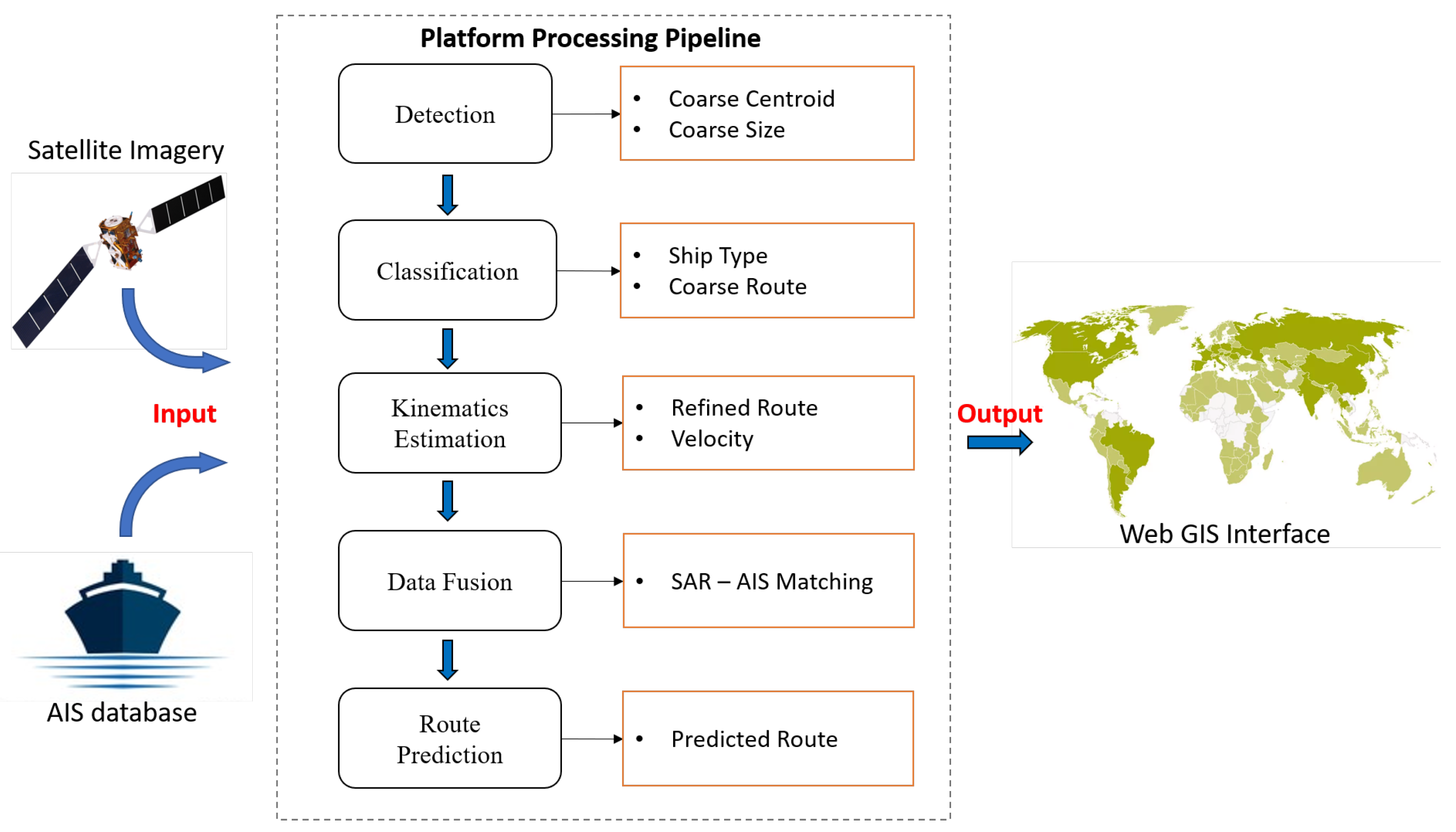
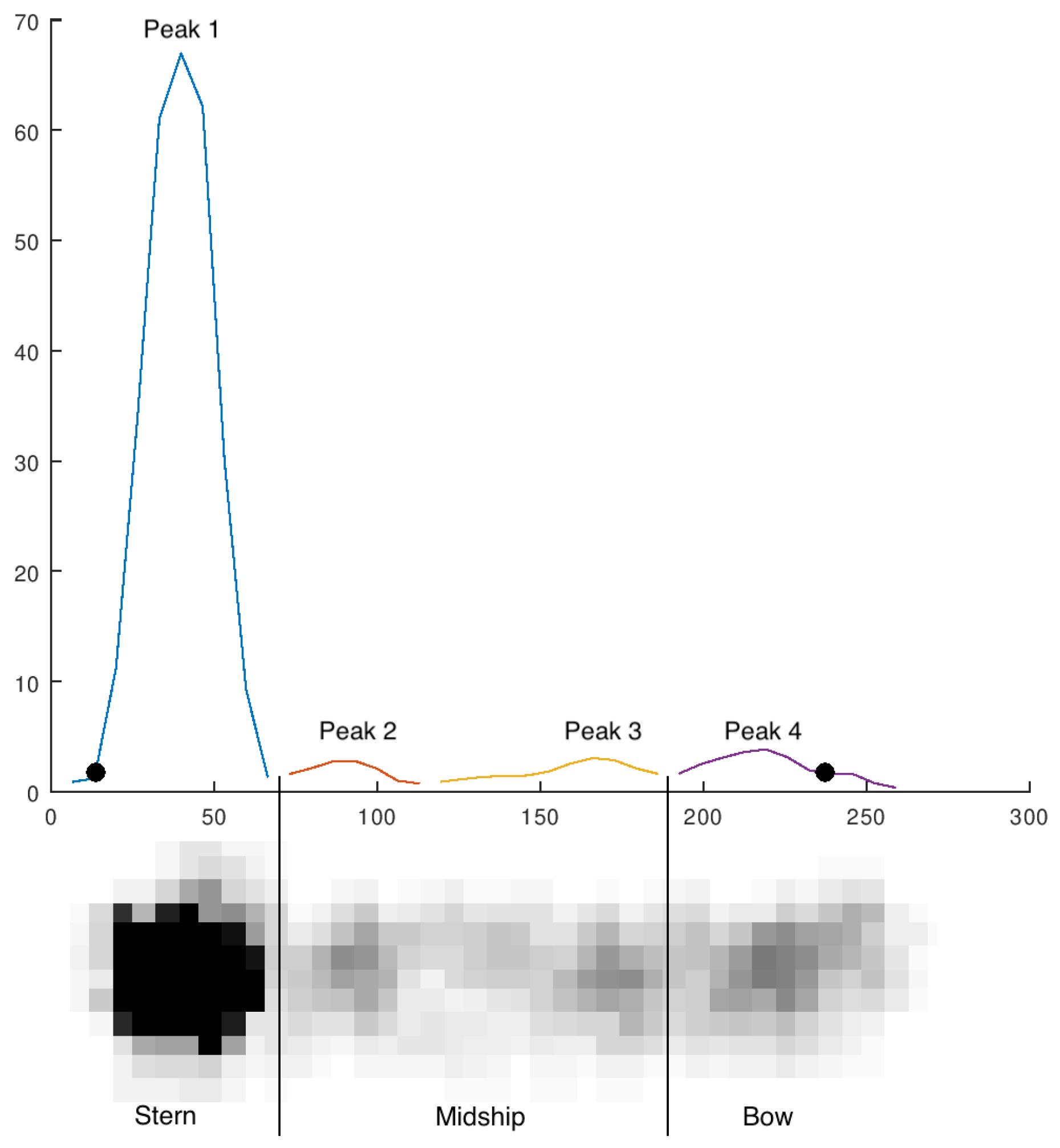
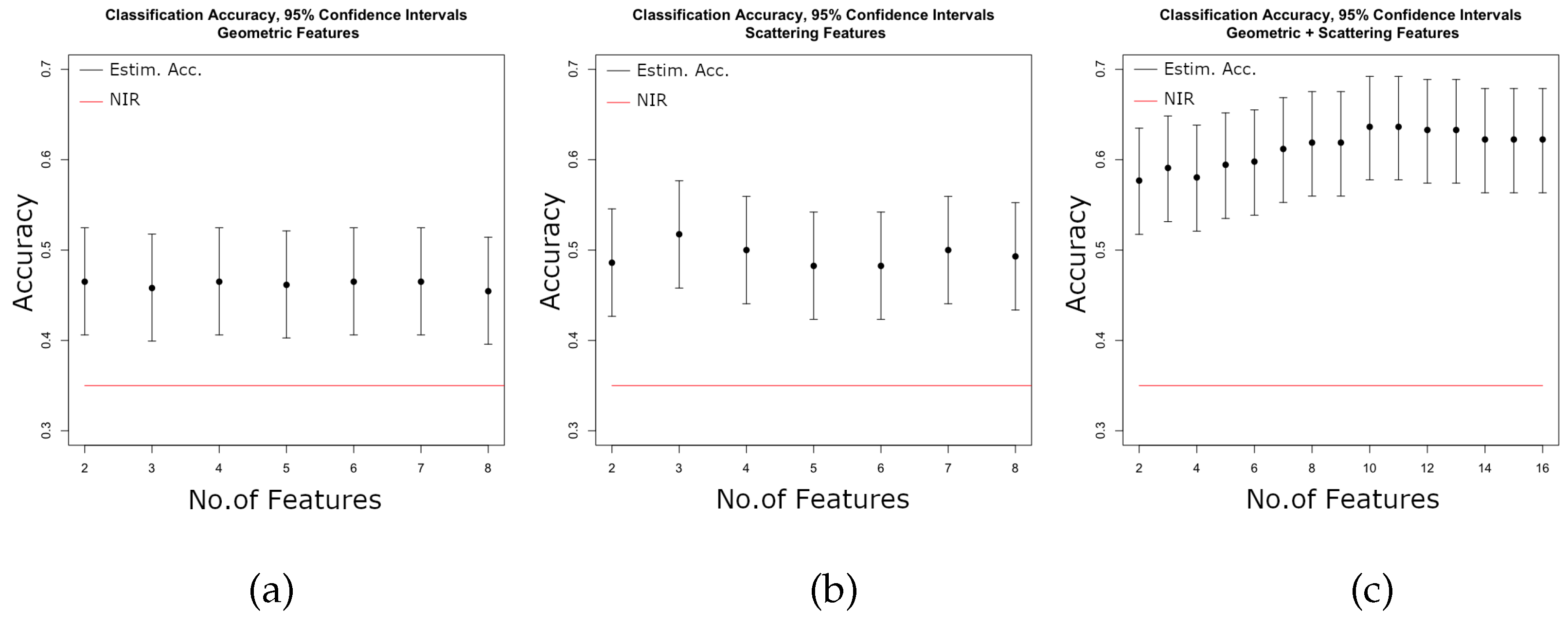
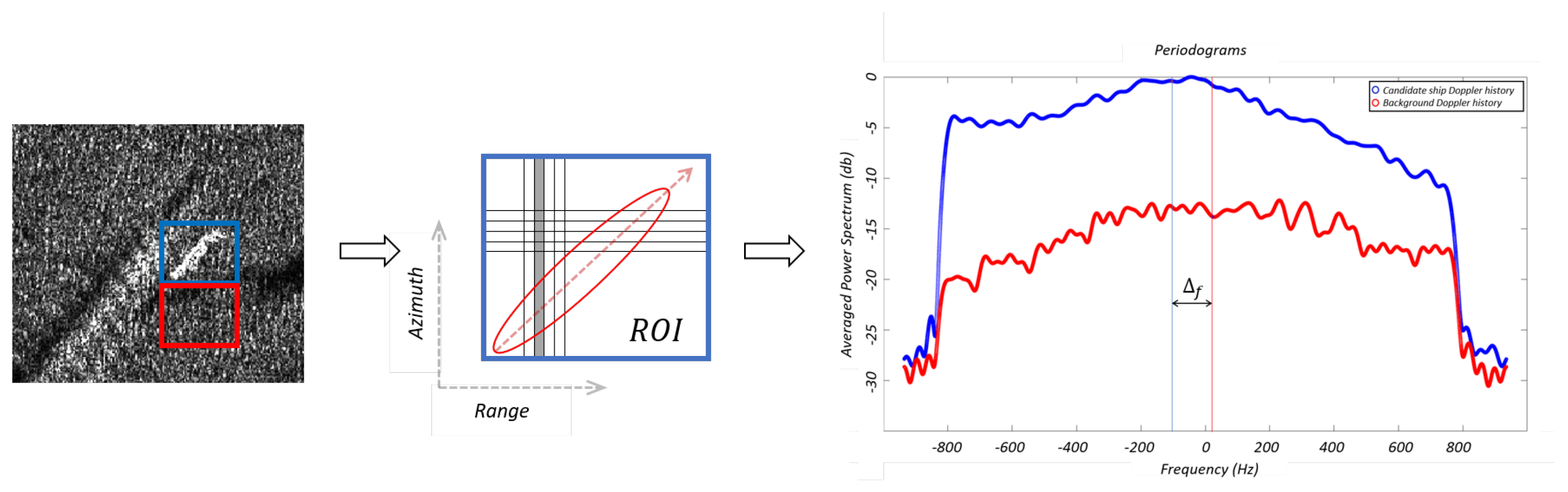
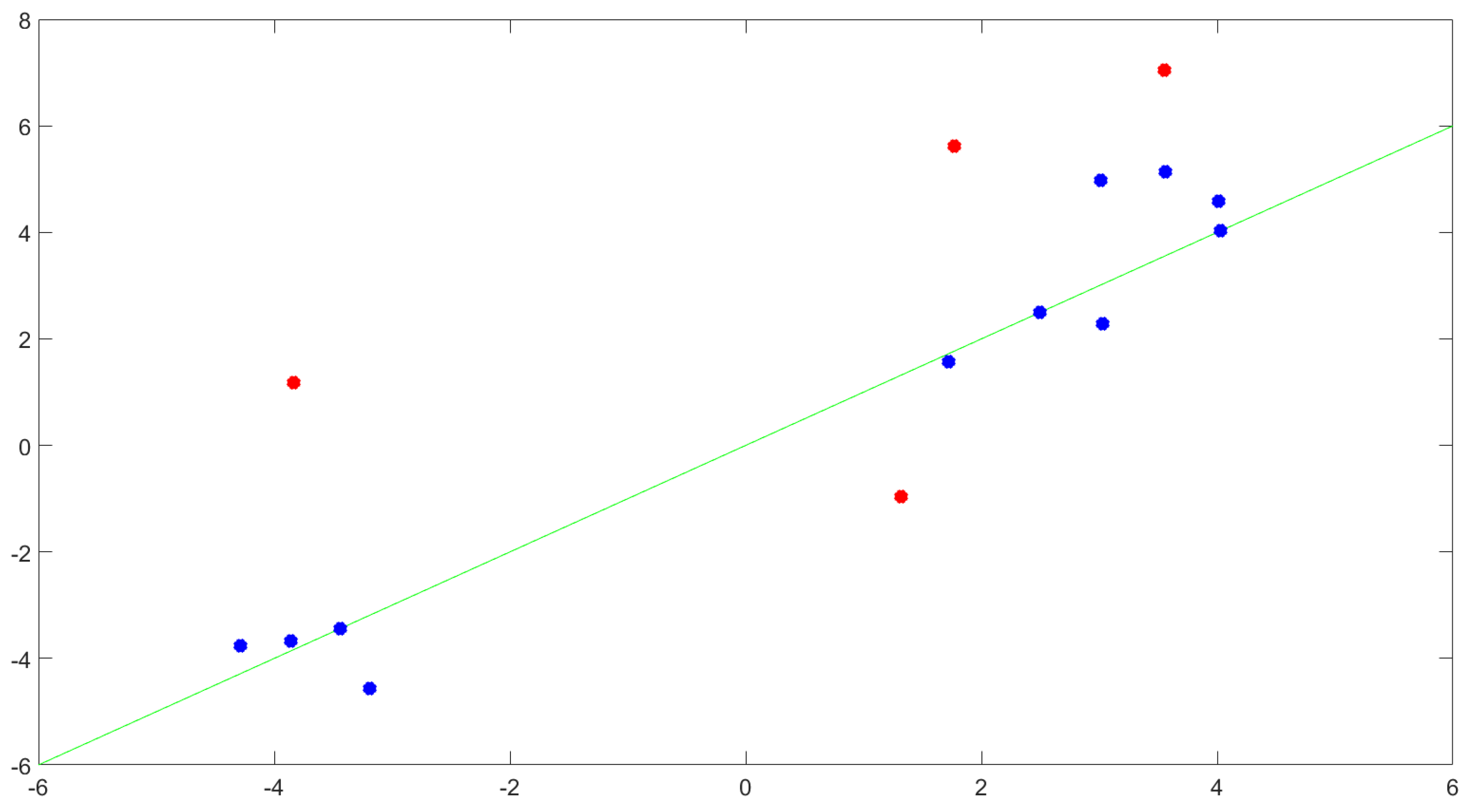
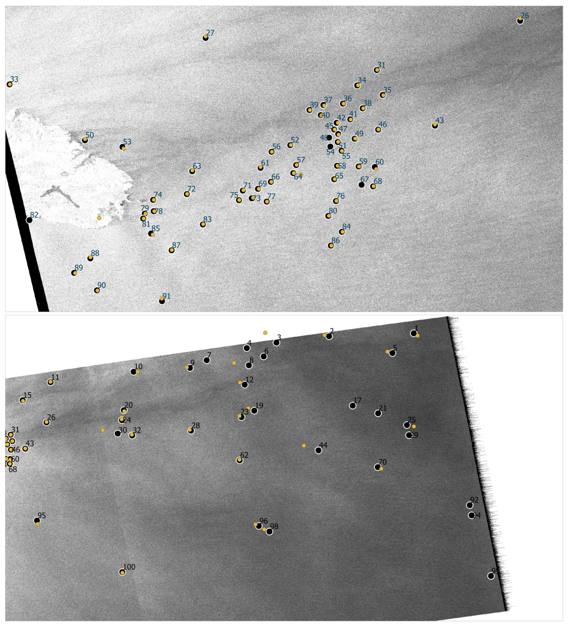
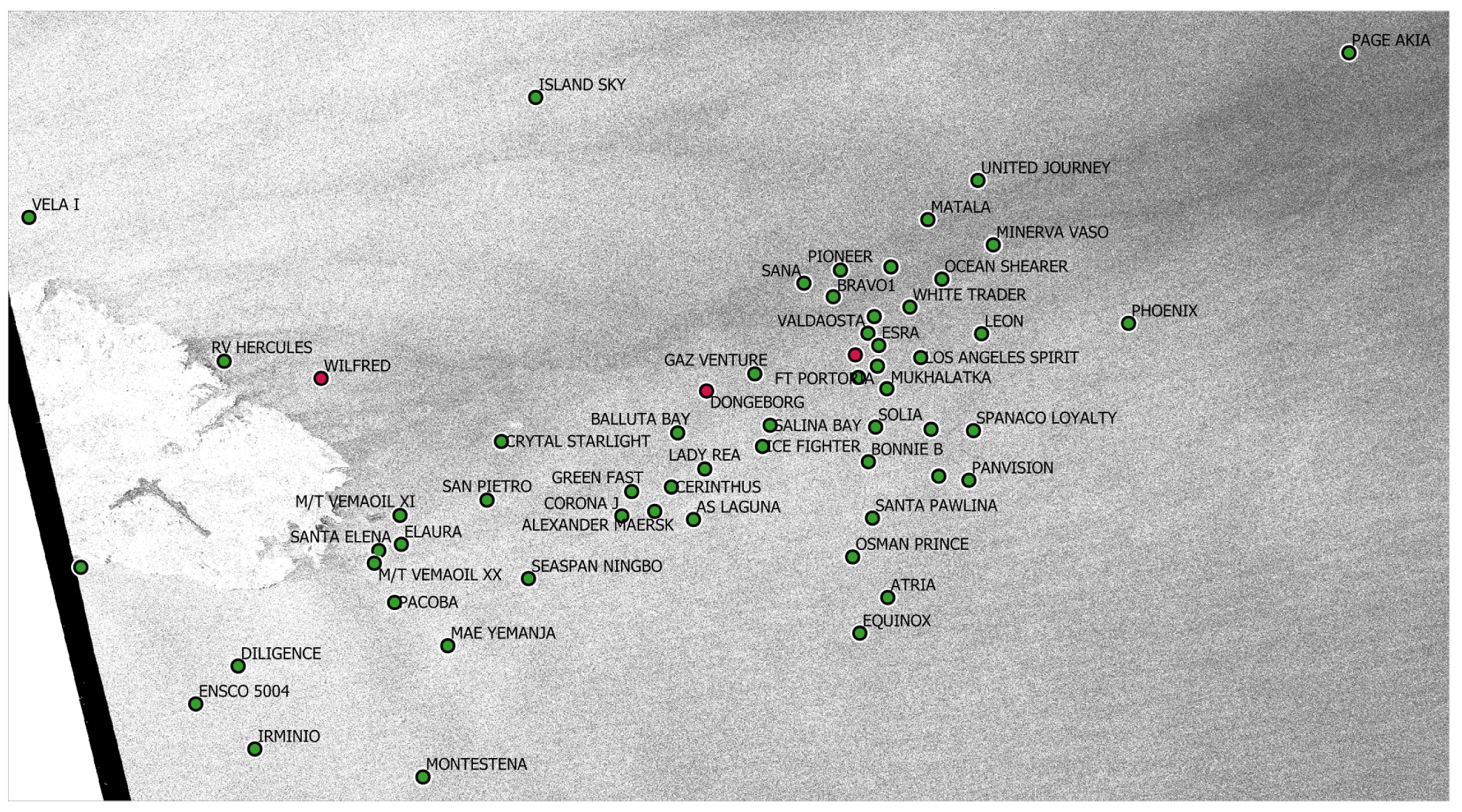
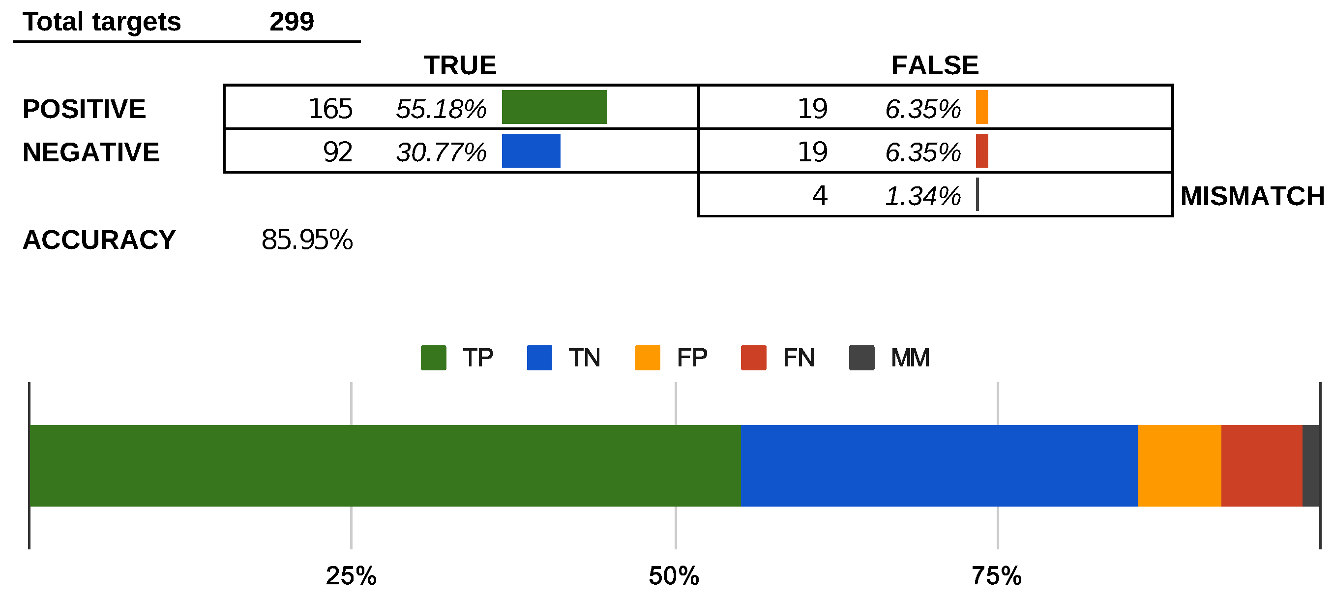
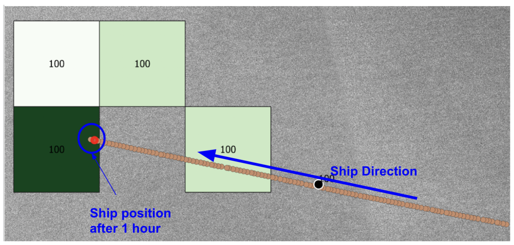