
Integrated Framework for Unsupervised Building Segmentation with Segment Anything Model-Based Pseudo-Labeling and Weakly Supervised Learning

Department of Civil and Environmental Engineering, Seoul National University, Seoul 08826, Republic of Korea
*
Author to whom correspondence should be addressed.
Remote Sens. 2024, 16(3), 526; https://doi.org/10.3390/rs16030526
Submission received: 12 December 2023
/
Revised: 18 January 2024
/
Accepted: 26 January 2024
/
Published: 30 January 2024
(This article belongs to the Section AI Remote Sensing)
Abstract
:The Segment Anything Model (SAM) has had a profound impact on deep learning applications in remote sensing. SAM, which serves as a prompt-based foundation model for segmentation, exhibits a remarkable capability to “segment anything,” including building objects on satellite or airborne images. To facilitate building segmentation without inducing supplementary prompts or labels, we applied a sequential approach of generating pseudo-labels and incorporating an edge-driven model. We first segmented the entire scene by SAM and masked out unwanted objects to generate pseudo-labels. Subsequently, we employed an edge-driven model designed to enhance the pseudo-label by using edge information to reconstruct the imperfect building features. Our model simultaneously utilizes spectral features from SAM-oriented building pseudo-labels and edge features from resultant images from the Canny edge detector and, thus, when combined with conditional random fields (CRFs), shows capability to extract and learn building features from imperfect pseudo-labels. By integrating the SAM-based pseudo-label with our edge-driven model, we establish an unsupervised framework for building segmentation that operates without explicit labels. Our model excels in extracting buildings compared with other state-of-the-art unsupervised segmentation models and even outperforms supervised models when trained in a fully supervised manner. This achievement demonstrates the potential of our model to address the lack of datasets in various remote sensing domains for building segmentation.
1. Introduction
Remote sensing has been a prevalent method for building segmentation tasks, playing a crucial role in urban planning, monitoring, and the development of smart cities. Technologies such as satellite or aerial photography enable image acquisition covering vast areas without physical presence, significantly reducing the cost of building masks and establishing remote sensing as a dominant method for building segmentation [1,2].
In recent years, the accumulation of very high-resolution aerial images and the launch of sub-meter optical satellites have improved the accuracy and building segmentation. Datasets such as ISPRS Potsdam [3], LoveDA [4], and SpaceNet [5]; building segmentation challenge datasets have been widely used in both remote sensing and computer vision to advance building segmentation algorithms. Recent progress in deep learning algorithms has further enhanced the accuracy and efficiency of building segmentation. Unlike traditional methods that rely on unstable features such as spectral information or building edges, a deep learning algorithm utilizes deep features for object segmentation. Encoder–decoder-based convolutional neural networks (CNNs), such as U-Net [6], Feature Pyramid Network [7], and DeepLab [8], have yielded breakthrough results in image segmentation. The encoder–decoder structure enables the model to learn deep features and classify the pixels to corresponding labels based on these features. Transformer-based models [9,10], adopting either the Vision Transformer (ViT) [11] or the Swin Transformer [12] on the model, have also demonstrated state-of-the-art performance, although with high computational cost and the requirement of large-scale datasets.
Despite the significant increase in dataset and technical resources, building segmentation remains challenging in various satellite or aerial images due to variations in spatial and spectral resolution. Existing datasets often fail to capture all these variations, and creating new datasets is often a labor-intensive task [13,14]. To address these limitations, training models with limited image resources have been extensively investigated. Unsupervised learning involves training models without labeled datasets [15,16,17], which is one such approach. Invariant Information Clustering (IIC) [15] transforms images through weak augmentation and segments them by maximizing mutual information between the features. Recent methods include self-distillation with no labels (DINO) [18], which was trained in a self-supervised manner. STEGO [16] used DINO as a backbone architecture to match corresponding features for segmentation, whereas HP [17] created the models that learned semantically similar pairs, known as global hidden positives, and used DINO as a feature extractor. However, unsupervised learning often results in less control over the model, and classification outcomes are highly dependent on the input data.
Another approach for training models with limited image resources is weakly supervised learning. This method typically involves generating pseudo-labels, initially through low-cost labels and subsequently training the segmentation model with these pseudo-labels in a fully supervised manner [19]. Pseudo-label refers to generating low-cost labels for unlabeled data that have the maximum predicted probability and utilizing low-cost labels for trainable input data as if they were true labels [20]. Low-cost labels in weakly supervised learning can be categorized as image- [21] and pixel-level labels, including scribbles [22], points [23], and bounding boxes [24,25]. Although image-level labels are cost-effective, they cannot infer high-quality and dense locations. Pixel-level labels, on the other hand, provide insufficient spatial information, often resulting in challenges related to recovering dense label structures. Edge features are commonly used as guidance in these tasks, but poor and insufficient edge-detection results can significantly degrade weakly supervised learning performance [26]. Therefore, generating pseudo-labels and implanting proper guidance to prevent overfitting is critical for weakly supervised segmentation.
Pseudo-labels in this context are generally obtained from superpixel segmentation [27] class activation map (CAM) [21,28] or pretrained models. Xu et al. [27] conducted an image classification approach using label constraint and edge penalty based on a superpixel algorithm. Li et al. [21] introduced a two-step segmentation network, which consisted of generating pseudo-labels and training, applying CAM and threshold to obtain the pseudo-label, and adopting CRF-loss [29] to enhance the pseudo-label. However, these tasks require image-level labels, and it is also difficult to infer high-quality and dense location information from image-level labels [30,31].
Meanwhile, the Meta AI research team, operating within the broader context of artificial intelligence at Meta (formerly known as Facebook), has proposed a foundation segmentation model named the Segment Anything Model (SAM) [32]. Trained extensively with a large amount of data, SAM demonstrates versatility in various domains, particularly in remote sensing applications. Ren et al. [33] conducted a comprehensive study, assessing SAM performance on various remote sensing segmentation datasets, including Solar [34], Inria [35], DeepGlobe and DeepGlobe Roads [36], 38-Cloud [37], and Parcel Delineation [38]. Their findings indicated that SAM exhibits comparable performance to the supervised model in building and cloud segmentation but faces challenges in road segmentation and parcel delineation, primarily due to occlusion in partial objects such as cars or buildings. SAM operates on a prompt-based mechanism, necessitating prompt or additional class information for the accurate annotation of segmented masks. While the model can automatically generate point prompts, the “segment anything” approach in spreading points from the background often leads to false positive segmentation.
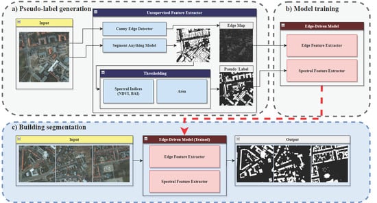
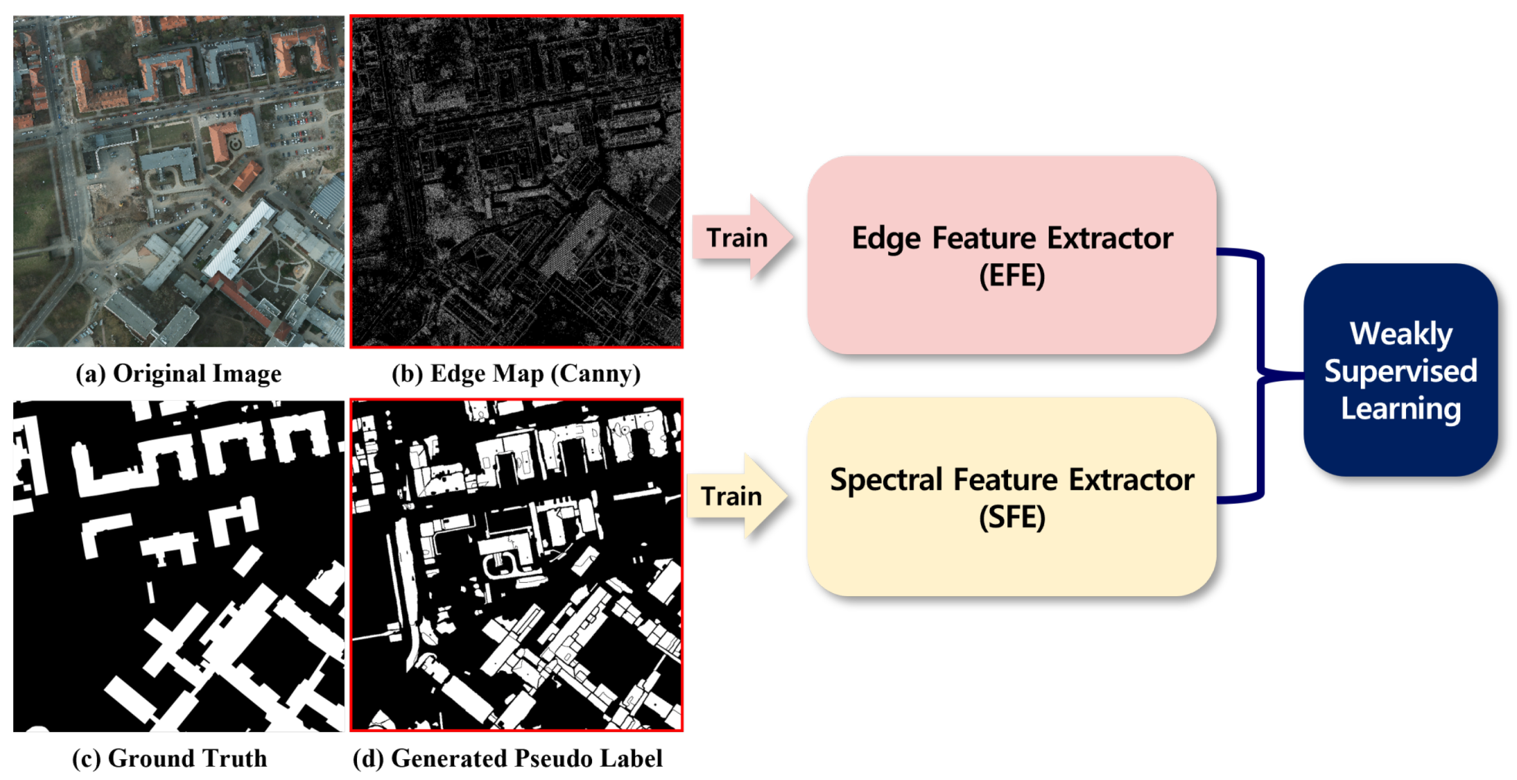
Based on the segmentation results of SAM, our research aims to create an unsupervised building segmentation framework using SAM and spectral index-based pseudo-labels coupled with a lightweight edge-driven weakly supervised model. Our framework follows the general weakly supervised learning structure for generating pseudo-labels and applying a weakly supervised model. However, unlike other weakly supervised learning frameworks, our approach generates pseudo-labels in an unsupervised manner, eliminating the need for datasets for the entire process. Our framework begins by extracting features using SAM and spectral indices. After extraction, these features are used as inputs for the weakly supervised models. The model uses edge information derived from the Canny edge detector [39] and generates a saliency map corresponding to classes based on this edge information. The saliency map guides object boundaries, preventing the model from overfitting to pseudo-labels. The results show that our model achieves greater accuracy in extracting buildings than previous unsupervised models for building segmentation. The overall process is shown in Figure 1.
2. Materials and Methods
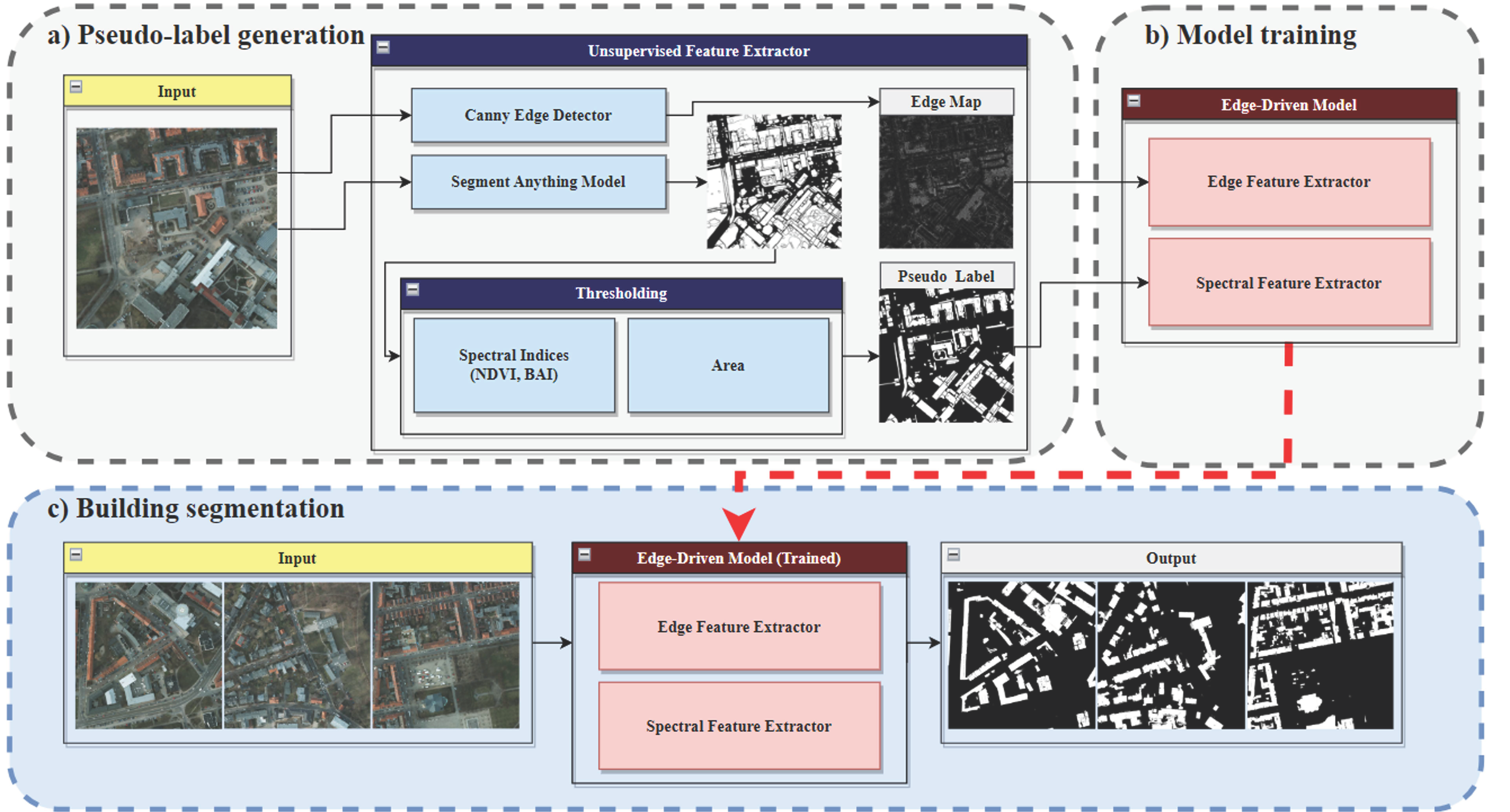
The overall process consists of two main subtasks: the unsupervised feature extractor and weakly supervised learning. In the first subtask, the unsupervised feature extractor extracts features from the image and generates pseudo-labels. This involves the use of SAM, spectral indices, and the Canny edge detector. Given that SAM tends to yield over-segmented results and that spectral indices necessitate thresholding for segmentation, a combination of area and index value-based thresholding was employed to generate the pseudo-label. Subsequently, in the weakly supervised learning phase, the pseudo-label and edge map were used as inputs to the proposed model. This model strategically uses the extracted edge features to prevent overfitting to the pseudo-label. To further enhance the results, conditional random fields (CRFs) [40] were applied as a post-processing step. The following subsections provide a detailed explanation of each step in the methodology.
2.1. Unsupervised Feature Extractor
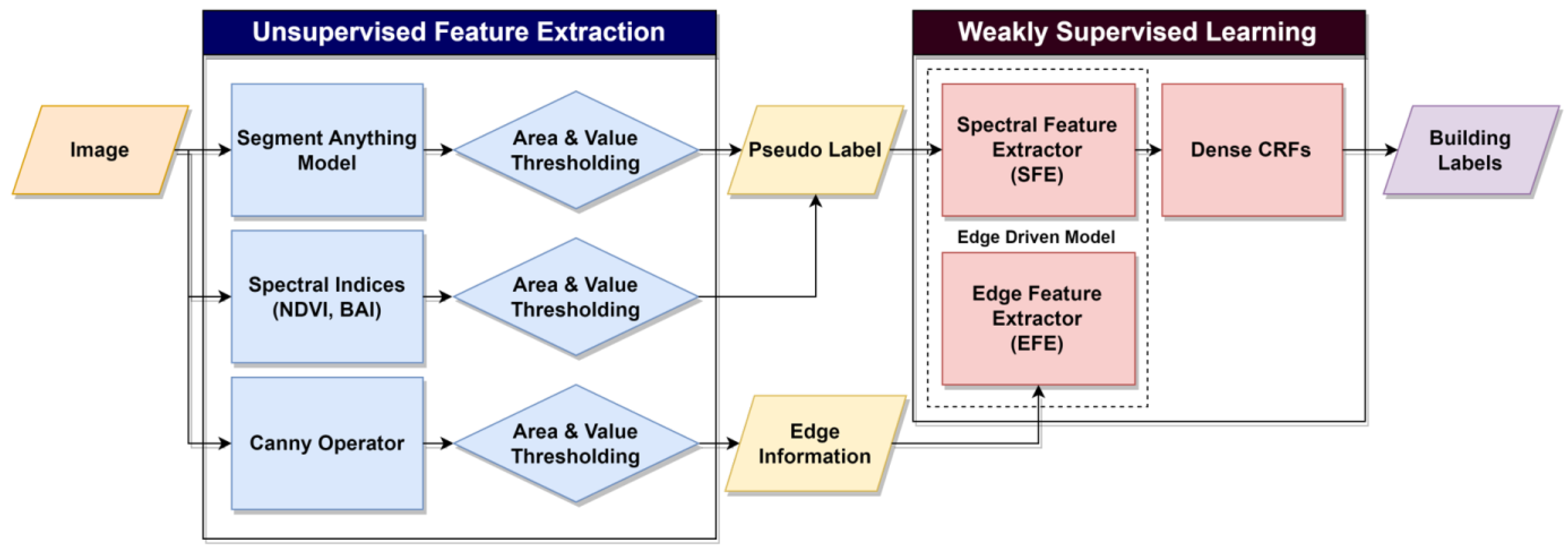
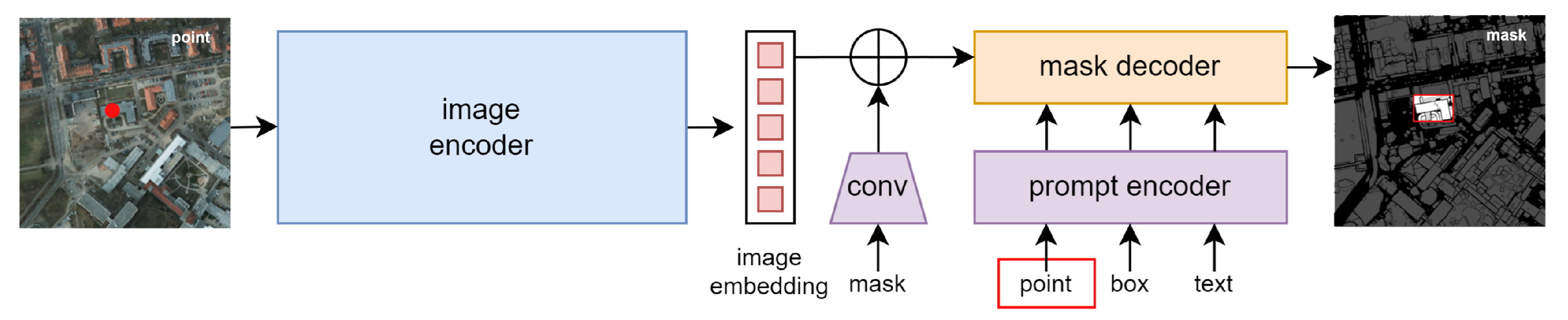
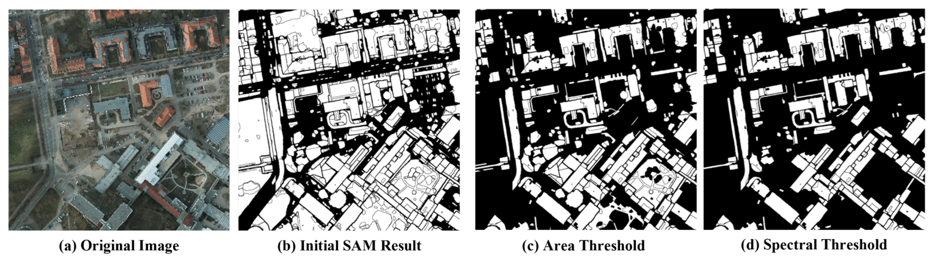
The foundation of our unsupervised feature extractor lies in the SAM, a well-established model for segmentation tasks. The structure of SAM can be seen in Figure 2. The model generates image embedding from the image encoder and the decoder producing segmented objects, queried by a variety of input prompts. The initial segmented objects obtained using the spreading point method are shown in Figure 3. The detailed inspection on initial segmented objects in Figure 3 demonstrates that SAM encounters challenges, notably in the omission and over-segmentation of objects. While SAM demonstrates proficiency in extracting various objects, its criteria for extracting cars and roads exhibit instability, leading to omission errors. In addition, although buildings are generally well-extracted, the model tends to over-segment buildings, creating multiple masks instead of a singular one.
To address these issues, we incorporate spectral index-based thresholding algorithms, which are known for being computationally straightforward [41] and for the independence from prior information on imagery [42]. Spectral indices, which leverage bands such as near-infrared (NIR), are widely used for classifying generated polygons. Given that NIR exhibits distinct radiation characteristics in water, vegetation, shadows, and other objects, it is frequently used for discrimination. One commonly used spectral index is the normalized difference vegetation index (NDVI), which is renowned for its effectiveness in emphasizing vegetation and is still applicable for dense vegetation detection. NDVI is widely employed for vegetation detection due to its algorithmic simplicity and the prevalent availability of the NIR band in remote sensing data; it is also known to be efficient when used as a low-cost pseudo-label [43]. In our approach, we applied an area and spectral index-based thresholding algorithm to annotate, mask out, and merge objects. Predominantly segmented objects include buildings, cars, trees, and roads. To refine the results, we implemented a heuristic thresholding algorithm, rejecting objects with sizes exceeding 2500 m2 or falling below 10 m2. This strategic thresholding significantly reduces the false-positive segmentation rate and enhances the Precision of the final results.
After applying area-based thresholding algorithm on polygons, we calculated the mean value of the spectral indices on the extracted polygons to mask out unwanted objects. NDVI and BAI [44] were sequentially applied to identify polygons in which vegetation and road predominate. Each object was then classified based on the heuristically determined threshold value. Recognizing that a heuristic approach to thresholding may introduce human intervention and bias into the model, we mitigated this by setting the threshold as low as possible, thereby minimizing commission errors. Given that our model operates on weakly supervised learning and uses edge information to distinguish objects, it does not entirely rely on pseudo-labels and is intrinsically robust to imperfect pixel label classes and threshold values. Therefore, the bias introduced by pixel classes from the heuristic approach can be disregarded to some extent. Considering the performance of the spectral index, building classes were first extracted, followed by the sequential removal of vegetation and roads. The result of the generated pseudo-label is shown in Figure 4.
where Blue, Red, and NIR refer to the brightness values of the corresponding bands: blue, red, and near-infrared.
While misclassified polygons are eliminated through the application of spectral indices, the pseudo-label results still exhibit various misclassifications. Consequently, although the model incorporates the generated pseudo-label during training, it must not solely rely on this information and requires additional data to prevent overfitting. To address this, we used the Canny edge detector to extract edge information from objects. The resulting edge information is used as guidance for reconstructing the building shapes. Compared with other well-known edge detectors, such as Sobel or Laplacian edge detectors, the Canny edge detector incorporates a Gaussian noise-filtering algorithm. This feature enhances the robustness of the result to speckle noises or rough textures, rendering it more reliable for guiding the identification of building structures [45]. Thus, the Canny edge detector was considered suitable for the edge extraction module.
2.2. Weakly Supervised Learning
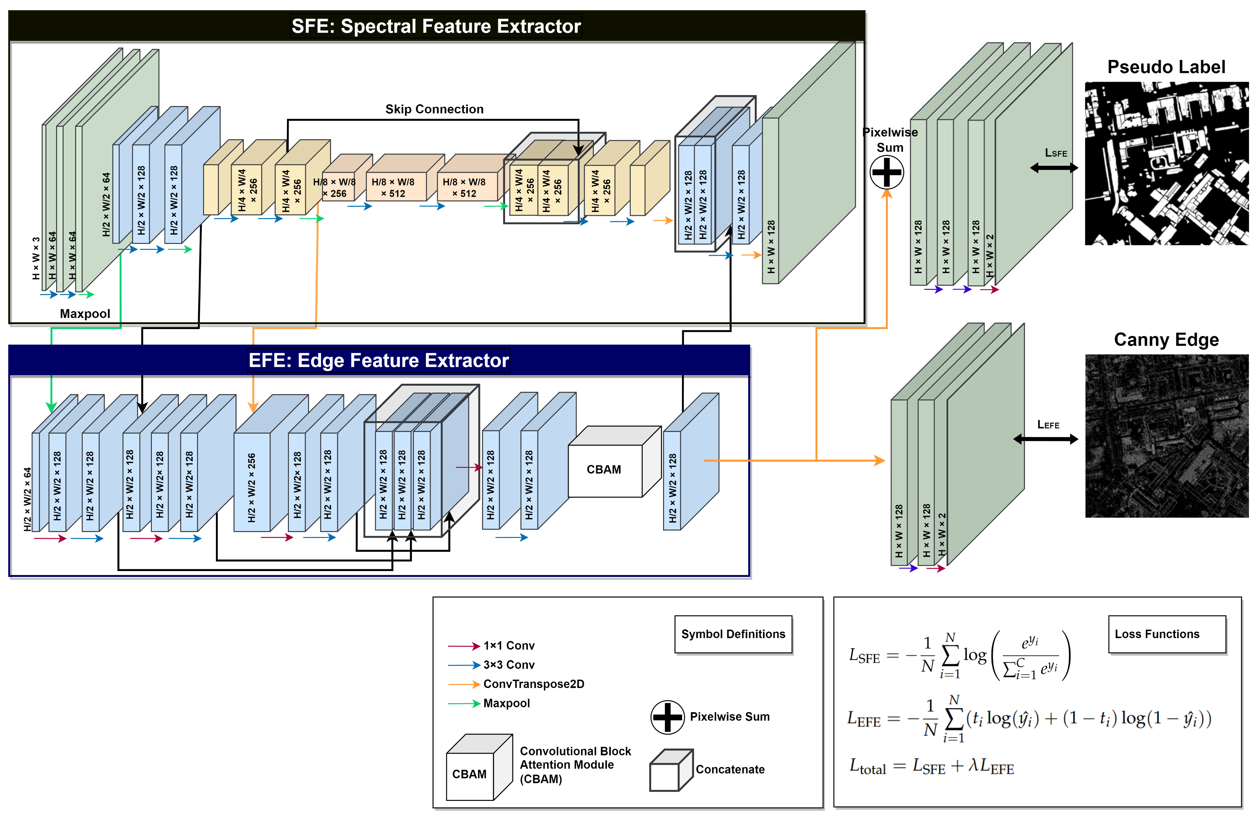
Drawing inspiration from the one-stage structure-aware weakly supervised network (SAWSN) [26], we incorporated edge information into our model to prevent overfitting and enhance shape accuracy. While the original model focuses on weakly supervised building extraction using scribble and edge inputs, our approach uses pseudo-labels instead of scribble. Moreover, our model is designed to be versatile and trainable in various domains, implying the need to represent various remote-sensing image domains while maintaining a lightweight structure that is suitable for training on a limited amount of data. Therefore, substantial modifications were made to our model, as illustrated in Figure 5.
Our model is designed with two major objectives, each associated with specific corresponding loss functions. The first objective involves pixel classification to assign pixels to corresponding objects, while the second focuses on generating object edges for the reconstruction of a building structure. To address these objectives, we introduce two branches: the Spectral Feature Extractor (SFE) and Edge Feature Extractor (EFE). The SFE is responsible for learning the classes of the objects at the pixel level and classifying each pixel. We use a standard CNN encoder–decoder structure for SFE, given the model’s training on a single remote-sensing image and the efficiency of CNNs with relatively small amounts of images compared with recent Transformer-based models. The loss function of the SFE is defined by Equation (3). Although most encoder–decoder structures use skip-connection structures to obtain spatial information, the role of SFE is concentrated solely on spectral features. Hence, we apply skip connection exclusively to the deepest convolution block, thereby obtaining the required spatial information from the EFE branch:
where and are the output and output after the sigmoid function, C is the number of classes, and N is the batch size.
The EFE branch’s primary role is to extract edge information from the features generated by SFE. To achieve this, EFE receives deep and shallow features from SFE and passes these features through a pooling block, consisting of 1 × 1 and 3 × 3 convolution blocks, and a scale adjustment layer to standardize features in terms of size and channels. After the pooling block, the layers are concatenated and further adjusted by passing through 1 × 1 and 3 × 3 convolution layers.
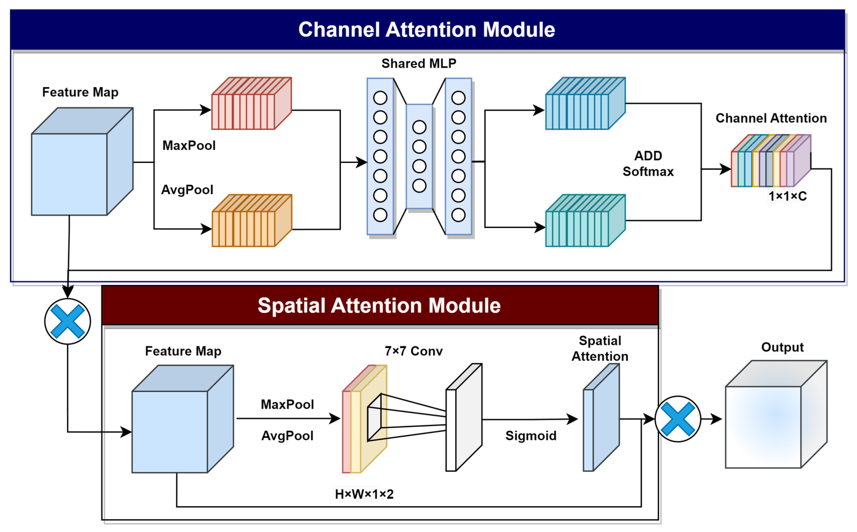
The EFE branch integrated attention mechanism is used to reduce the weight of unwanted edge features. The attention mechanism enhances the model’s performance by gaining information on key elements. There are two general types of attention mechanisms, which are channel attention (CA) and spatial attention (SA). CA refers to the channel dimensions of the input features and assigns different weights according to the importance of each channel. Similarly, SA refers to giving different weights to different spatial locations in a feature map. The Convolutional Block Attention Module (CBAM) [46] integrates both attention mechanisms. CBAM consists of two sequential channel and spatial sub-modules, using max and average pooling on both channel and spatial dimensions to generate an attention map (Figure 6). The CBAM module plays a fundamental role in the EFE branch of our model, emphasizing important features and de-emphasizing unimportant edge features, thereby making the model robust to the edges of small objects.
After passing through an additional pooling block and sigmoid function, the result is compared to the edge label generated by the Canny edge detector. The loss function for EFE and are defined in Equations (4) and (5), respectively:
where , are the output and output after the sigmoid function, C is the number of classes number, is the value of the true label, N is the batch size, is the weight for adding the loss function.
The EFE branch induces edge information, generating sharper building segmentation results and preventing overfitting to pseudo-labels. However, this method also incorporates point edge noises on the results and makes the model susceptible to edge noises. We implement dense conditional random fields (CRFs) for enhancing the building edges while reducing noises. The objective of applying dense CRFs in our model is to enhance the pseudo-label without requiring additional human-annotated labels, resulting in improved sharpness and accuracy of the edges in the segmentation results. CRFs are a class of probabilistic graphical models that have proven to be effective in various machine learning tasks, particularly in image segmentation. CRFs model the relationships between pixels through two types of potentials: unary and pairwise. Unary potentials capture the individual likelihood of each pixel belonging to a particular class, which is often derived from pre-trained classifiers or deep neural networks. Pairwise potentials encode the interactions between neighboring pixels by considering the pixel-to-pixel relationship. The total energy function E could be defined as the summation of unary and pairwise potential, and our goal could be defined as the minimization problem of the energy function E:
where is unary potential calculated from our model, is pairwise potential, x represents the set of binary building labels, and i and j represent the pixel location.
The equation for unary potential and pairwise potential can be defined using Equations (8) and (9). Unary potential is calculated from our trained model and pairwise potential is calculated from the relationship between nearby pixels:
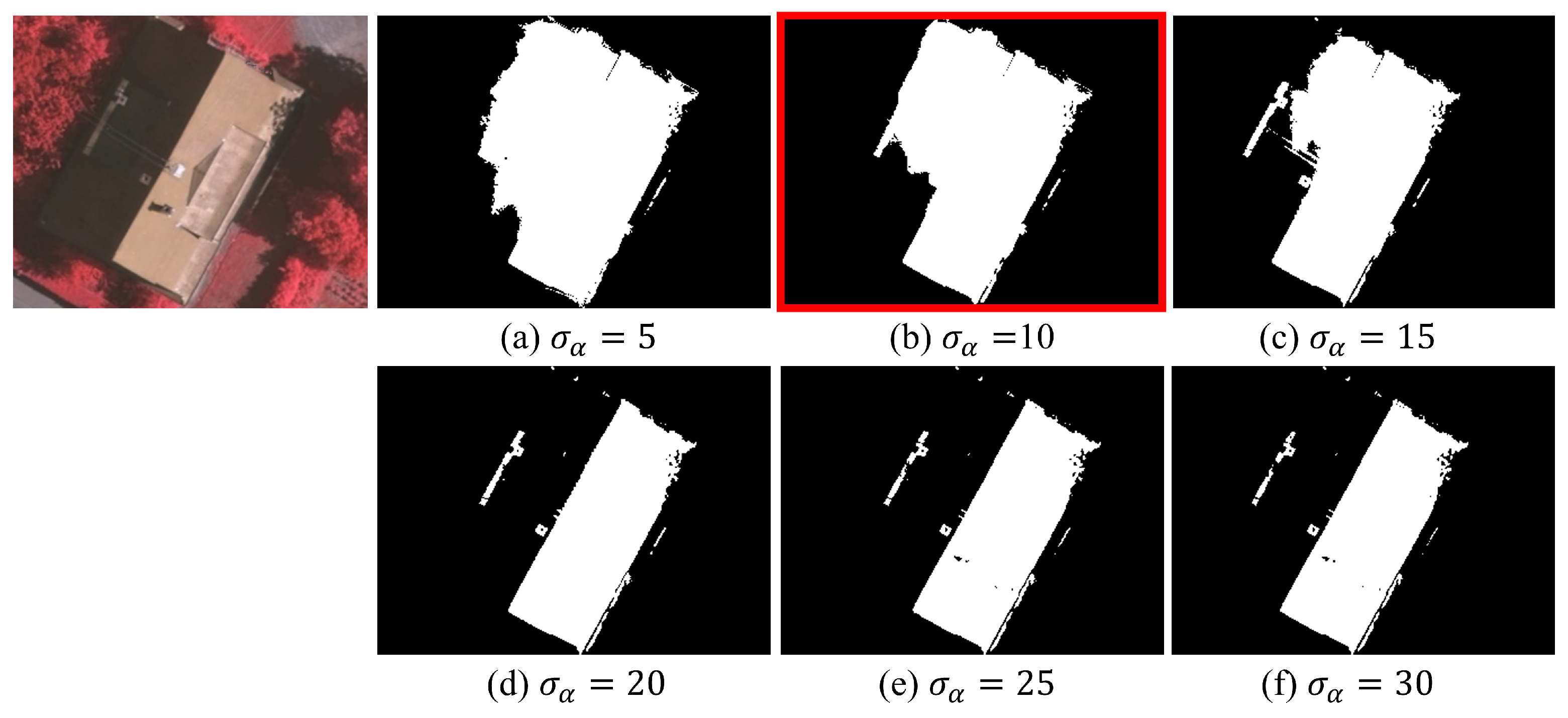
is the binary term that penalizes the nearby pixels with different labels: if , and otherwise zero. The term calculates contrast between two nearby pixels with summation of appearance kernel and smoothness kernel, with weight of and for each. The appearance kernel uses the difference in their positions p and the information of pixel color I, controlled by the standard deviation of and for each. The smoothness kernel uses pixel proximity to remove small isolated regions and give the mask a much sharper boundary, controlled by the degree of smoothness with standard deviation value of . The terms , , and are adjusted to match the purpose. was set low to focus on high-frequency building edges and was set high to consider color variety in roofs. was set low for localized smoothing. This fine-tuning on Figure 7 optimizes the CRF’s impact without additional labeled data, ensuring precise corrections to the model’s predictions, particularly in capturing building details while mitigating potential inaccuracies.
3. Experiments
3.1. Datasets
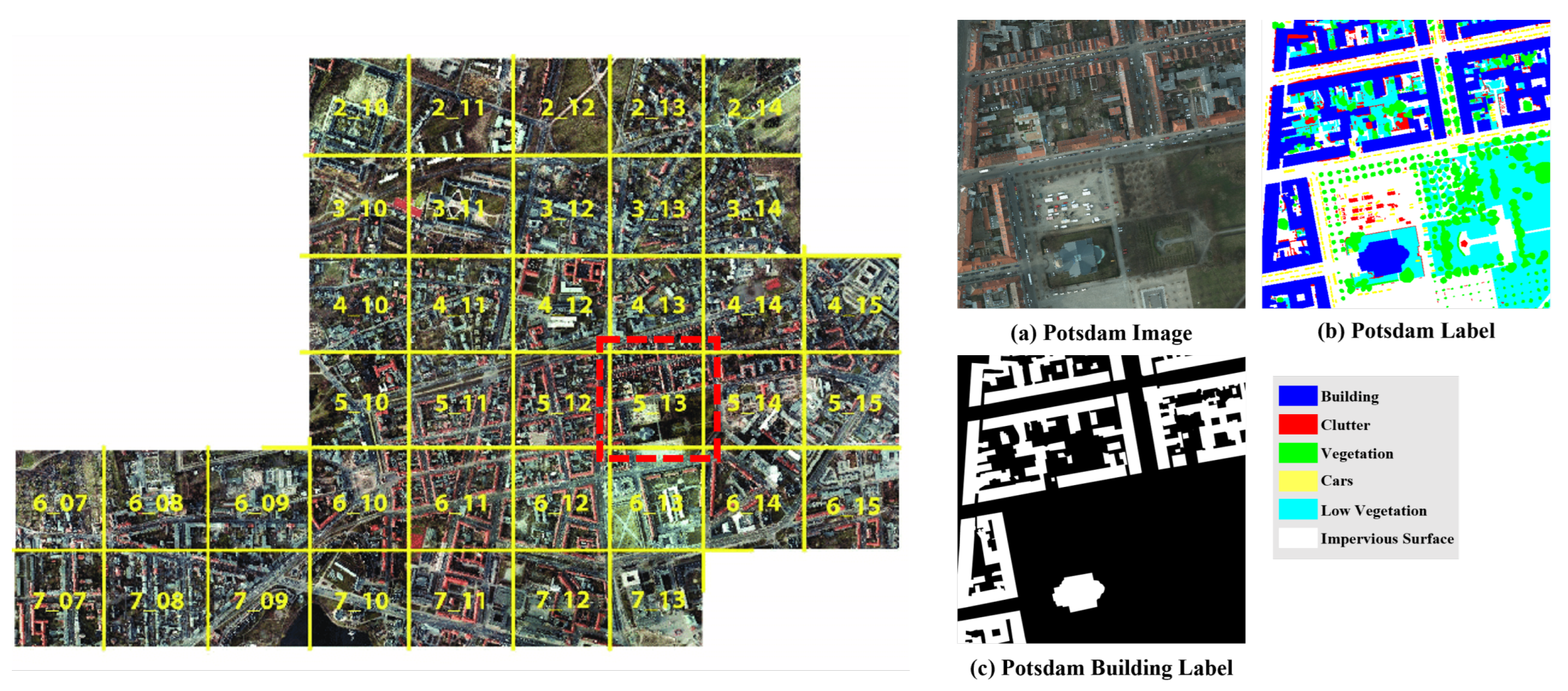
Our approach eliminates the need for human-annotated ground-truth labels during training. Labels were exclusively used to evaluate the unsupervised segmentation results and model performance. For evaluation, we used the building class of the Potsdam dataset (Figure 8) and Vaihingen dataset. The Potsdam dataset consists of 38 patches with size of 6000 × 6000, with 6 classes: building, clutter, tree, low vegetation, car, and impervious surfaces. The spatial resolution of the dataset is 0.05 m, and the images are accurately orthorectified. This dataset is widely used in various segmentation tasks, including unsupervised building segmentation, vegetation segmentation, and road segmentation. In our experiments, we used 24 patches of the Potsdam dataset for training and reserved the remaining 14 patches for evaluation purposes. The patches were divided into size of 500 × 500, and one out of nine train patches was used for validation. Thus, 3072 out of 3456 divided patches were used for train and the remaining 384 patches were used for validation. The 2016 divided patches were used for evaluation.
The Vaihingen dataset consists of 33 patches with 6 classes: building, clutter, tree, low vegetation, car, and impervious surfaces. The spatial resolution of the dataset is 0.09 m and the dataset includes a digital surface model within the file. The Vaihingen dataset has 3 bands of red, green, and near-infrared. Among the 33 patches, the Vaihingen dataset has 16 labeled patches for evaluation, which were used for evaluation in our research. We also divided the patches into size of 500 × 500, and one out of nine train patches were used for validation. Thus, 249 out of 280 divided patches were used for train and the remaining 31 patches were used for validation. The 241 divided patches were used for evaluation.
3.2. Evaluation
In our evaluation process, we chose the f1-score and IoU (Intersection over Union) for comparison. These metrics are among the most widely used evaluation measures in segmentation tasks. The f1-score determines the harmonic mean of Precision and Recall. Precision is defined as the ratio of accurately predicted positive results to the total number of positive results predicted by the model. Conversely, Recall denotes the ratio of true positive results to the total number of actual positive results. By calculating the harmonic mean, the f1-score can indicate whether the segmentation rate of the model is balanced. We also used IoU to follow the tradition of evaluating building segmentation. IoU refers to the ratio of the intersection area between the ground-truth and predicted masks to the union area of the two. The metric is expressed in Equation (14):
where TP represents true positives, FP corresponds to false positives, and FN denotes false negatives.
3.3. Training and Validation
In terms of training strategies, we incorporated Gaussian noise augmentation and random crop augmentation. Given that our model classifies pixels based on SAM-based pseudo-labels and reconstructs building structures using edge information, introducing edge information to the model inherently makes it susceptible to point or edge noise. Gaussian noise augmentation was applied to enhance the model’s robustness to noises. For random crop augmentation, we cropped the image size to 500 × 500 and then randomly cropped them to 384 × 384. For the training strategy, the weight in Equation (5) was set to 0.2, and a learning rate of 0.001 was used with the Adam optimizer [47]. The batch size was set to 8, and the model was trained on a single NVIDIA GeForce RTX 2080 Ti GPU with 8 GB memory using the PyTorch library. DINO backbone models, HP and STEGO, and ResNet50 backbone models, IIC and MANet, were initialized in pretrained weights, and the rest were initialized in Kaming initialization [48].
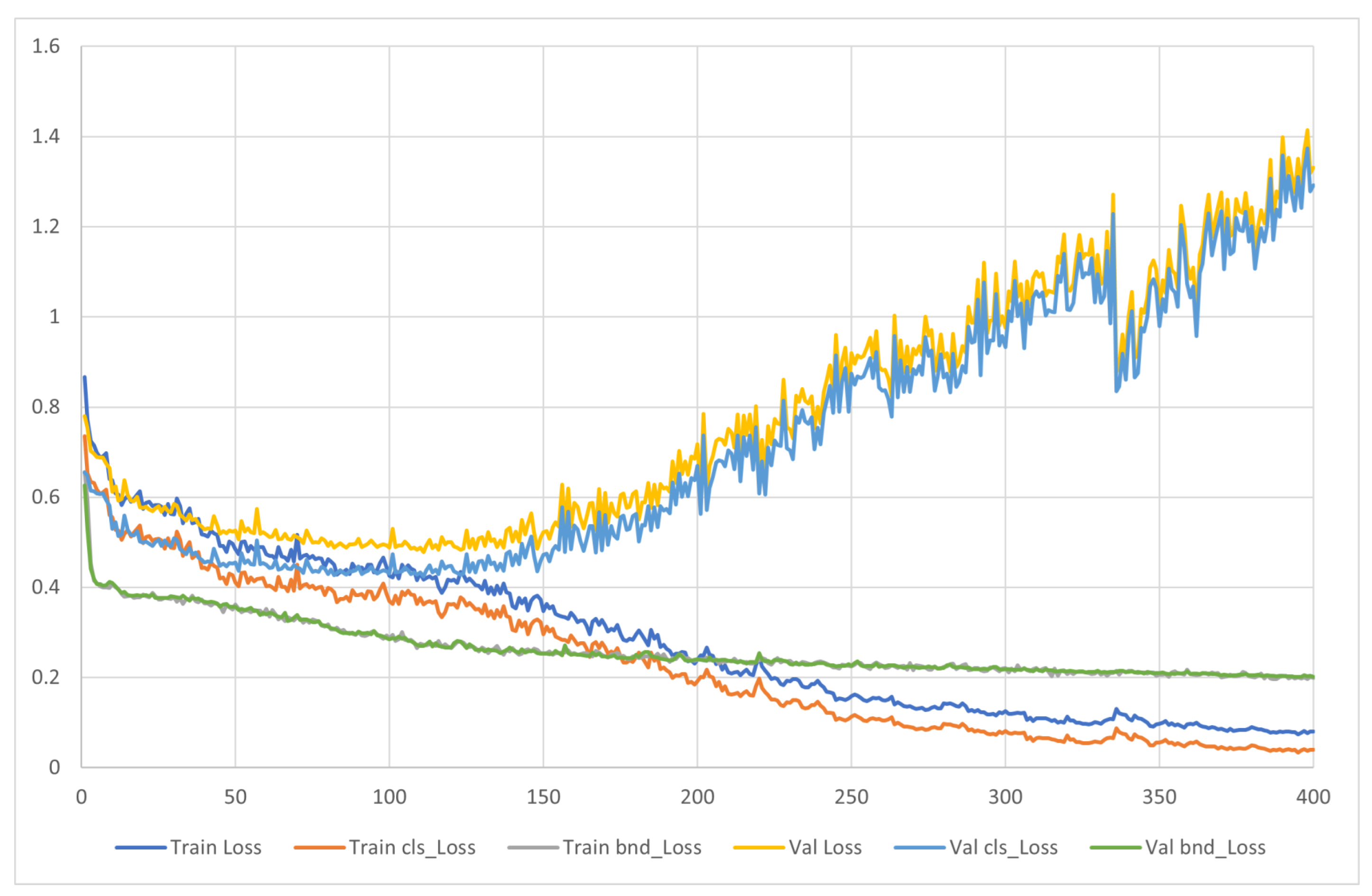
Figure 9 represents the corresponding loss value of our model. The validation loss is calculated within the generated pseudo-label and edge map. Our model has two loss functions: , which is boundary loss, and , which is classification loss. Each represents the loss value for boundary and spectral information and guides the model to focus on corresponding features. The analysis of the loss value implies that, though the boundary loss keeps decreasing, classification loss reaches a minimum value from epoch 100 to epoch 150. Therefore, to balance between the two corresponding losses, the model with lowest validation score was saved and used for evaluation.
3.4. Experimental Results
We conducted a comprehensive comparison with the state-of-the-art unsupervised segmentation model, IIC [15], STEGO [16], and HP [17]. IIC [15] uses contrastive learning based on weak augmentation and is a CNN-based model with superior accuracy in unsupervised segmentation, particularly on the Potsdam dataset, while STEGO and HP are state-of-the-art vision Transformer-based models that show great accuracy on the Potsdam dataset. Furthermore, to assess the inherent performance of our model, we conducted a comparison by training it with a fully supervised dataset and compared the results with those obtained from fully supervised models. For this purpose, four well-established models, namely U-Net [6], DeepLabV3+ [8], Deep Residual U-Net [49], and MANet [50] were selected. We then compared the results of these models with our results, which were trained on a supervised dataset.
3.4.1. Unsupervised Models
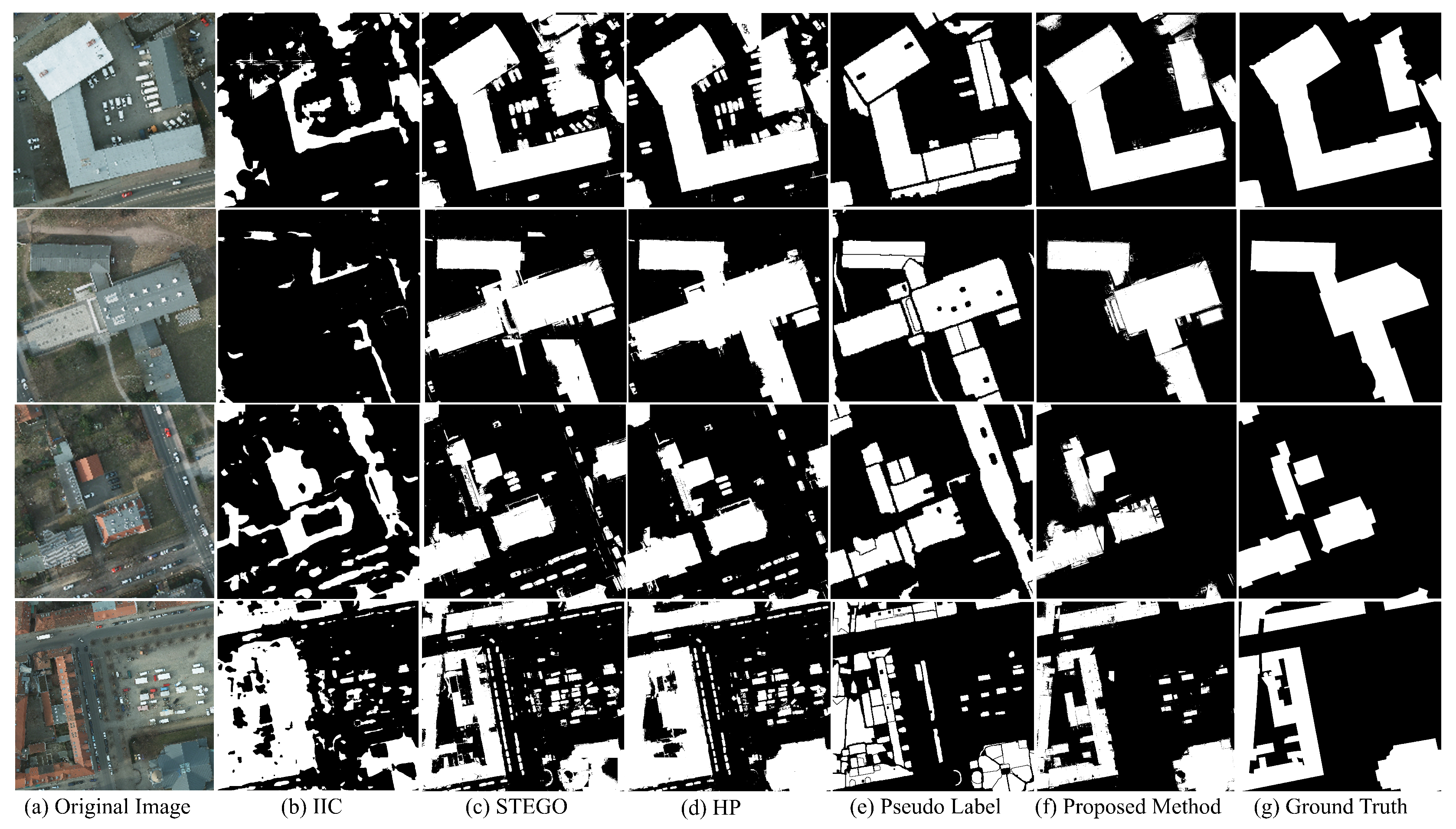
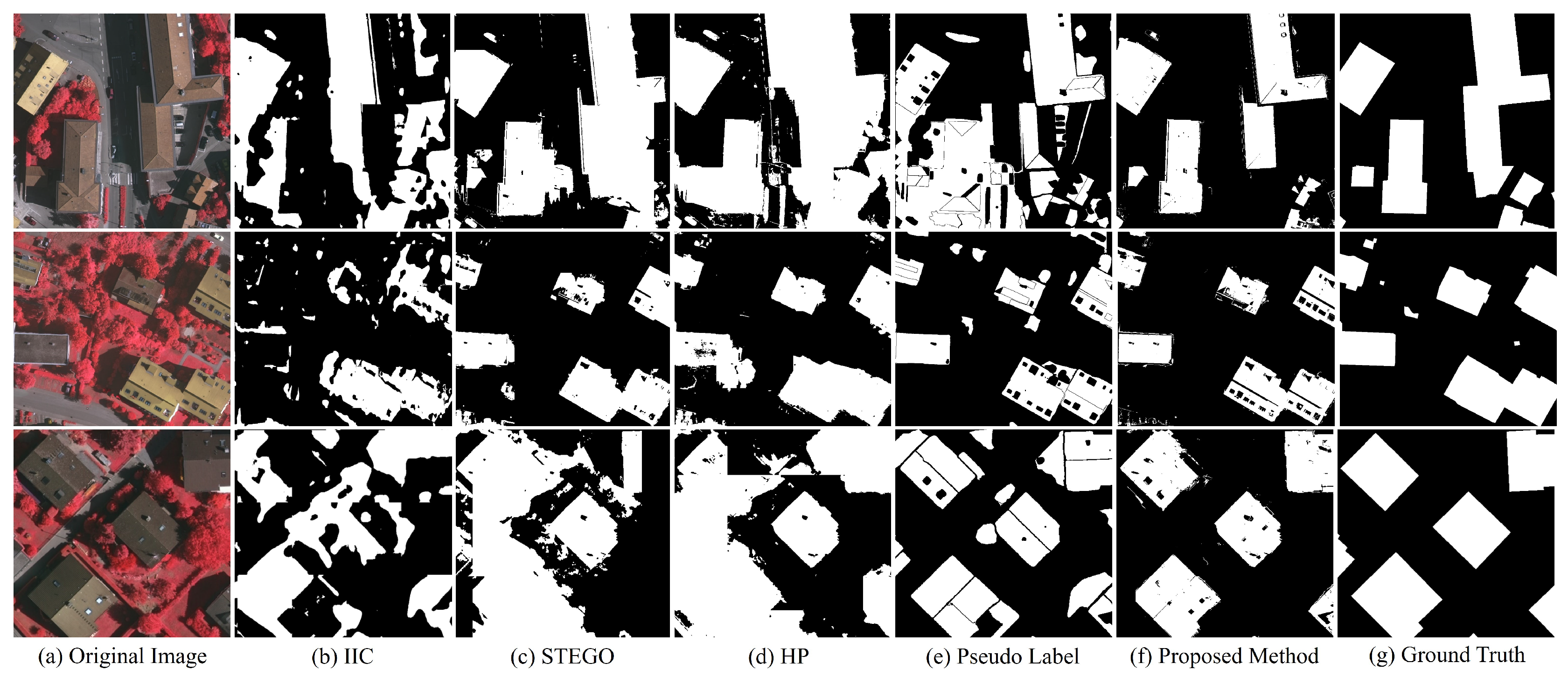
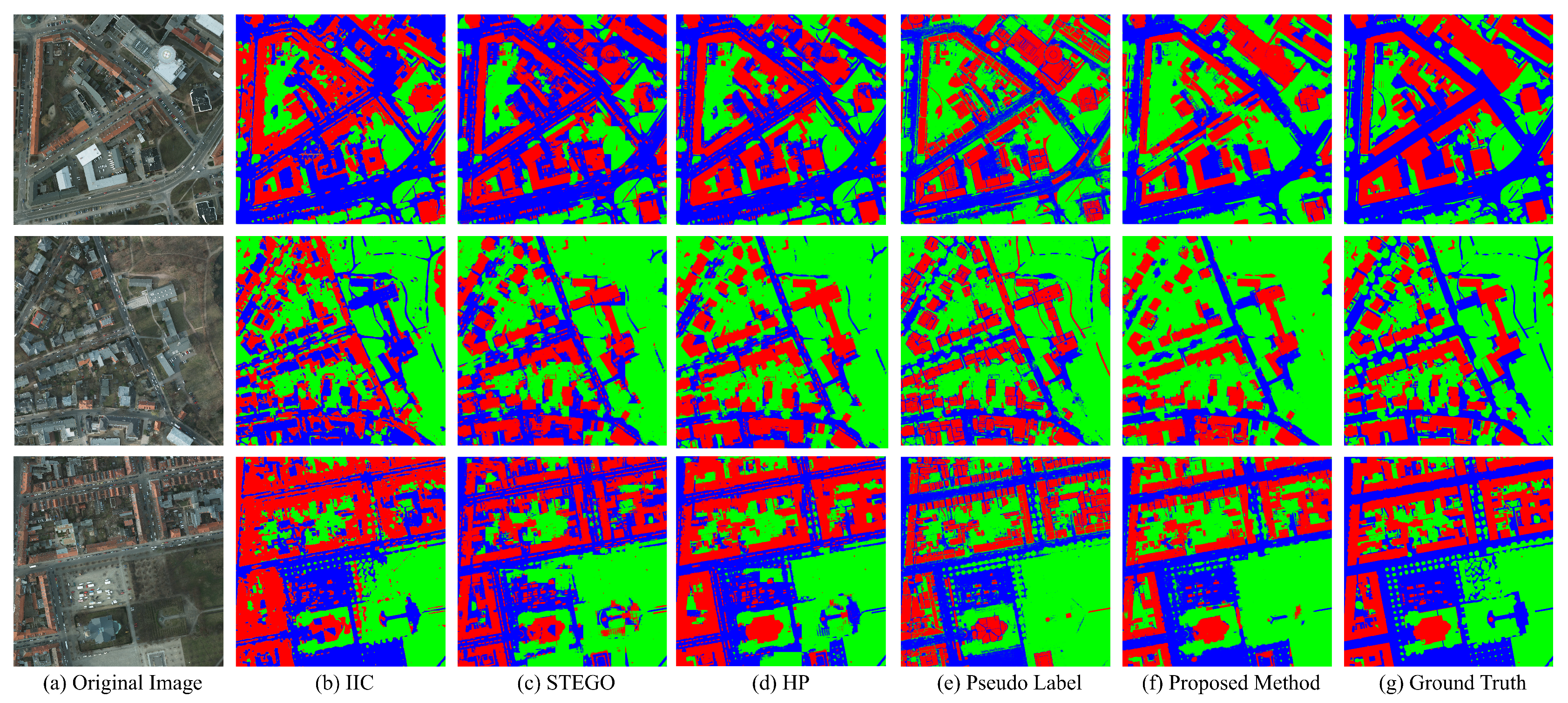
The visual comparison and quantitative evaluations of the unsupervised models on the Potsdam dataset are presented in Figure 10 and Table 1. Notably, our model outperforms other models, achieving the best results in building segmentation, with an f1-score of 0.78 and IoU of 0.64. Compared with STEGO and IIC, our model significantly reduces the misclassification rate of pixels. Unsupervised models often rely on the similarity or contrast of extracted features, potentially leading to a lack of control over the training process. However, our model uses the pixel features derived from SAM-based pseudo-labels, providing a guiding framework for building classification. This approach enhances control over the learning process, resulting in an overall improvement in building segmentation accuracy.
IIC encountered challenges in consistently generating reliable building segments. The primary factor contributing to this issue was the inherent instability in the criteria for identifying building objects. IIC derives features by discerning contrasts between original and weakly augmented images, thereby rendering the segmentation of buildings with diverse roof features into a singular class exceptionally challenging. Consequently, IIC selectively recognized only those buildings exhibiting specific roof features, while dismissing those with alternative roof types. While the outcomes were comparatively improved, similar issues were observed in the context of STEGO and HP. In the case of STEGO, there was an incorporation of cars within the building class, and a simultaneous exclusion of buildings with specific roof types. Similarly, though discrimination of buildings was slightly better than STEGO, HP also incorporated cars within the building class. In contrast, our proposed model demonstrated a noteworthy distinction by acquiring a comprehensive understanding of generic criteria applicable to various roof types.
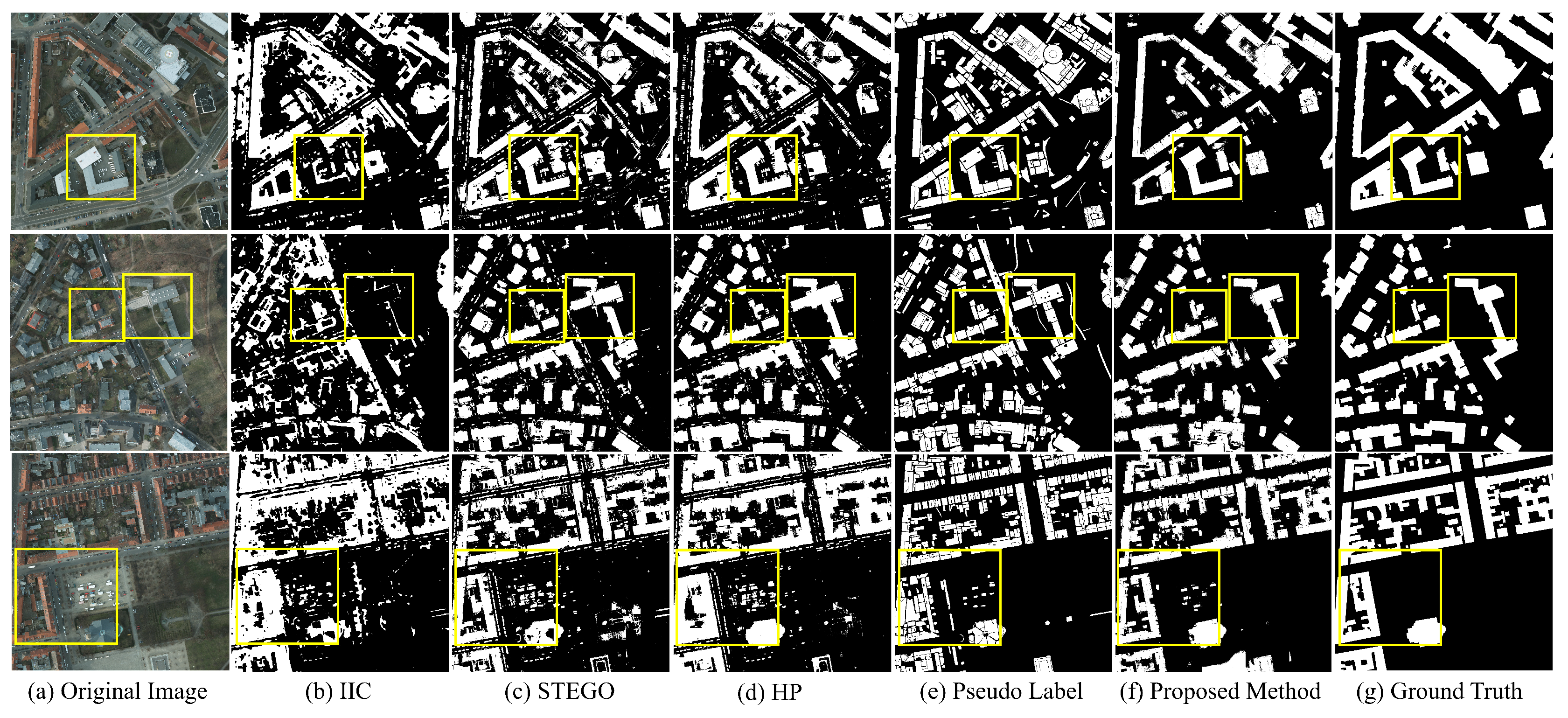
The similar results could be observed in Vaihingen dataset on Figure 11 and Table 2. The results show that our model greatly outperforms the other models, especially in label consistency and discrimination of building edges. The visual comparison on Figure 11 proves that our model shows exceptional consistency in generating building segments, while others frequently failed to create accurate building segments. Though pseudo-label proved reliability on preserving the building edges, it often included other objects, leading to decrease in Precision score. The quantitative comparison on evaluation metrics also proves that our model is capable of generating building segments regardless of image domain. Considering that the images from Vaihingen dataset consists of NIR, R, G bands instead of R, G, B bands and spatial resolution of 0.09, instead of 0.05 m, our model consistently expressed better results than other models even when the image domain changed.
An important highlight of our model is its substantial improvement over the accuracy of the pseudo-label, which serves as a trainable dataset for our weakly supervised model. Visual comparison on full images, Figure 12, between the pseudo-label and our proposed method reveals a significant reduction in misclassified pixels clusters, contributing to increased Precision, f1-score, and IoU. The increase in Precision score was exceptional, from 0.7066 to 0.8242, which implies that the overly generated building segments were greatly reduced after being trained by our model. The result shows that edge information derived from the Canny edge detector not only guides building shape reconstruction but also prevents overfitting to the pseudo-label, thereby enhancing general pixel classification performance.
3.4.2. Supervised Models
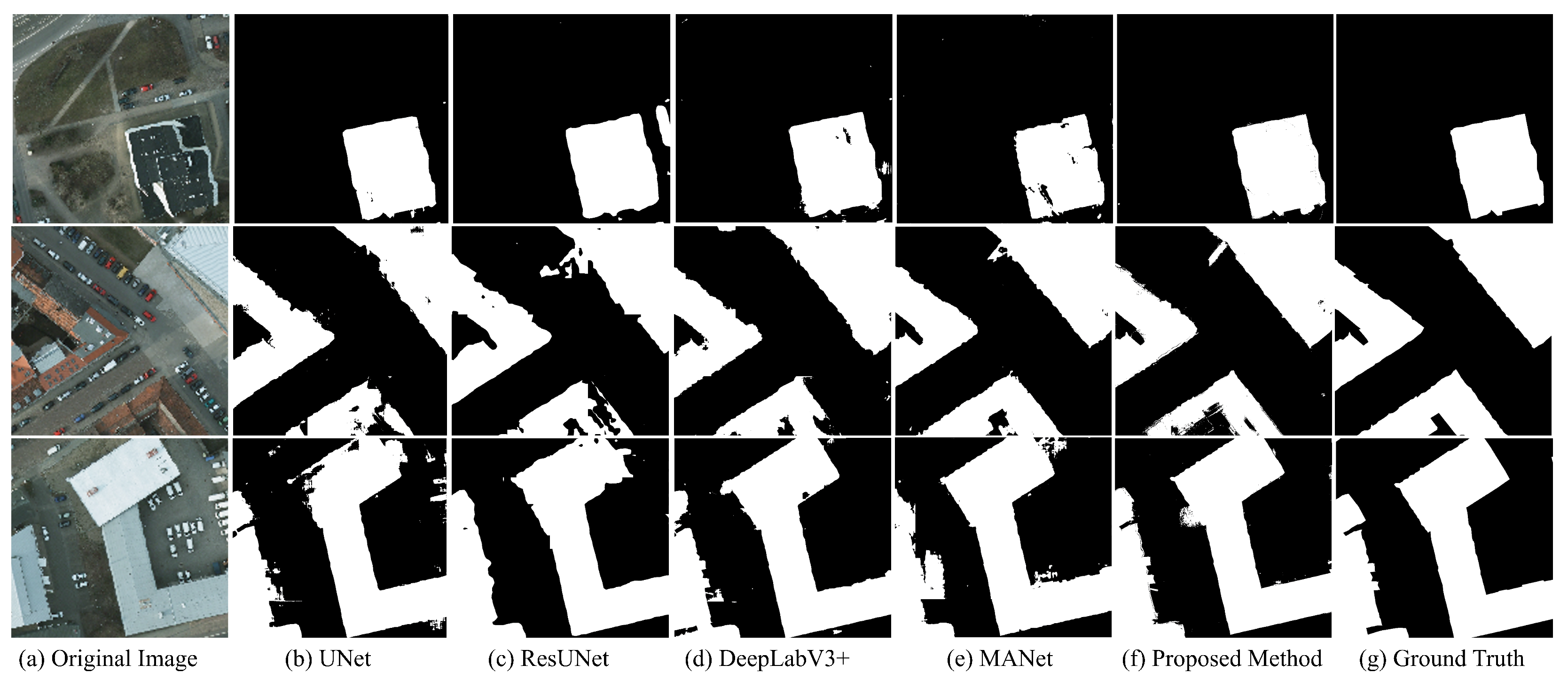
The comparison of our model with the unsupervised model implies that our model shows great performance compared with the other unsupervised segmentation models. However, the segmentation accuracy was due to the great improvement in clusters of misclassified pixels rather than the model’s delicate ability to preserve edges. To solely evaluate the performance of our model, we trained our model on a fully supervised manner and compared it with other fully supervised models (Figure 13, Table 3). The visual inspection in Figure 13 implies that our model also shows comparable performance on building segmentation compared to supervised models. The major factor that affected the increase in accuracy was the great improvement in preserving edges. Compared to other models, our model directly uses edge information on training, and this generally increases the performance on the segmentation of building boundaries.
In a quantitative analysis, our model yielded comparable outcomes to MANet and ResUNet. MANet achieved f1-score of 0.8540, Precision of 0.8601, Recall of 0.8536, and IoU of 0.7481, and ResUNet achieved f1-score of 0.8504, Precision of 0.8687, Recall of 0.8381, and IoU of 0.7427. Our model achieved similar value in f1-score and IoU but exhibited higher Precision of 0.9072 and lower Recall of 0.8080. These metrics show that our model has a tendency to produce fewer building segments and yields high Precision yet lower Recall. The performance of DeepLabV3+, which similarly integrates a CRF module for post-processing, also exhibited great edge results, with f1-score of 0.8344 and IoU of 0.7216. However, the consistency of results was much better in our proposed model. DeepLabV3+ effectively retained the building edges but demonstrated a tendency to classify pixels within the confines of building boundaries, generating noises inside the segmented objects, while our model consistently classified pixels in a stabilized manner.
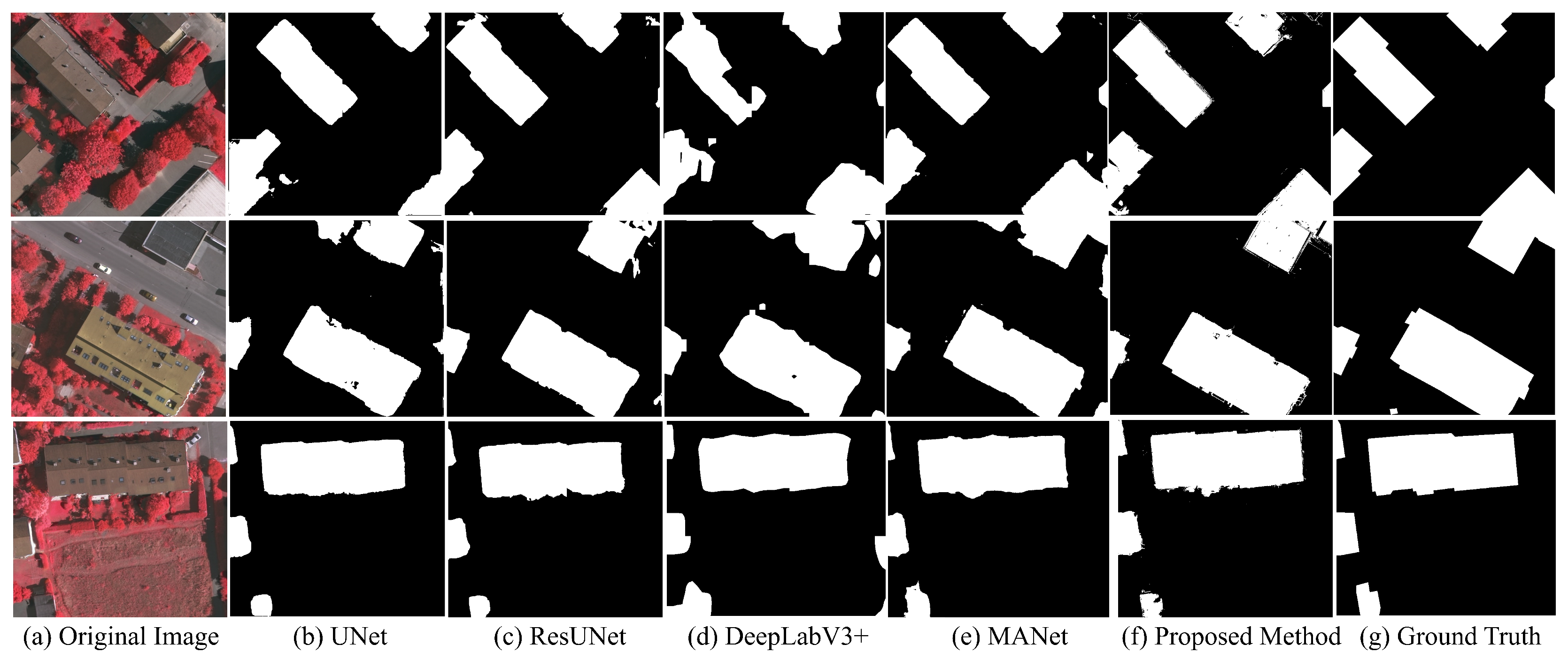
Similar trends could be also observed in the Vaihingen dataset (Figure 14, Table 4). On visual inspection, our model greatly preserved the edges of buildings compared to other models. MANet and ResUNet also proved great ability to preserve building edges but both were not as sharp as our model. Our model provided the best accuracy, with f1-score of 0.8435 and IoU of 0.7295, with higher Precision score and lower Recall score compared to ResUNet and MANet. Our model directly uses edge information on the model for edge refinement, and this led to increase in Precision, while reducing the Recall parameter.
4. Discussion
Comparison with both unsupervised and supervised segmentation models reveals that our building segmentation framework outperformed its unsupervised counterparts and was also capable of being trained in a fully supervised manner. On comparison between unsupervised models, our model proved excellence in discrimination of building objects, with f1-score of 0.7829 and IoU of 0.6463. State-of-the-art unsupervised models rely on contrast or similarity of building features, and this often led to unstable criteria for discrimination of buildings. Our model, on the other hand, utilizes pseudo-labels for training and shows better performance in discriminating building objects. Notably, our model also exhibited better performance than the pseudo-label itself that was used to train our model. The edge information improved the edges of pseudo-labels and increased stability in discrimination of buildings.
We further compared our model with fully supervised models to analyze the performance of our model itself. Unsupervised models tend to generate clusters of misclassified pixels and hinder the analysis on model itself. Our model utilizes edge information on training and thus exhibits excellence on preserving edges. The result also proved the ability of our model to preserve exact boundaries of buildings. On visual inspection, we found out that the edges of buildings were greatly improved on our model, while other models often generated noises on building edges. DeepLabV3+ which also…building edges: removed.
Though our model exhibits exceptional performance on both supervised and unsupervised models, several questions remain unclear. First, inducing edge information clearly shows efficiency in improving pseudo-label, implying that the limit to which the model receives and utilizes the edge information should be explicitly identified. Second, pseudo-label was generated from SAM polygons with spectral index and area threshold, but the generalized efficiency of utilizing edge information to enhance inaccurate pseudo-label should be analyzed. Finally, the model was designed to be trained on pseudo-labels, which are often insufficient in quantity, and, thus, the model should have few parameters. Therefore, in this section, we conducted several studies to deeply investigate our framework and compensate for the remaining questions.
4.1. Effects of Edge Information
The incorporation of edge details significantly increased overall accuracy in both unsupervised and supervised contexts, providing crucial shape information to the model. To balance between the loss from pseudo-labels and the informative edge data (as defined in Equation (5)), we introduced a weight parameter that was set to 0.2. However, to identify the optimal utilization of edge information and understand the model’s interpretation of such details, we systematically varied the weight. By applying different weight values, we assessed how edge information influences the model’s performance. The result could be seen on Figure 15 and Table 5.
In examining the relationship between model weight and evaluation metrics, the inclusion of edge information consistently demonstrated an enhancement in the Recall parameter. Initially, with zero weight (no edge information), the model exhibited a Precision of 0.8196 and a Recall of 0.6306, implying an inclination to less-labeled buildings. Upon incorporating edge information, the Recall metric exhibited a notable improvement, ranging from 0.6740 to 0.7429, indicating the successful guidance of the edge information in reconstructing building shapes and reducing unnecessary segmentation.
Despite the considerable boost in Recall through the incorporation of edge information, the Precision parameter exhibited independence from changes in weight. No discernible pattern emerged regarding the impact of weight on Precision. Specifically, a weight of 0.2 significantly exceeded the Precision of zero weight, while a weight of 0.5 led to a substantial decrease. The intended role of edge information in reconstructing building structures faced challenges due to variations in the results of the Canny edge detector, particularly concerning different roof types. For instance, rough roof textures did not consistently reveal clear roof types, impacting the Precision parameter, as edge features did not consistently align with building boundaries. Consequently, the application of edge information contributed to increased Precision to a certain extent, but an excess of information led to a decrease in Precision.
Similar trends were observed in f1-score and IoU. Weight values of 0.2 and 0.3 exhibited superior performance, yielding f1-scores of 0.7828 and 0.7641 and IoUs of 0.6463 and 0.6207, respectively. However, a decline in performance occurred upon reaching a weight of 0.5, resulting in an f1-score of 0.6714 and an IoU of 0.5099. Notably, the decrease in Precision at higher weights surpassed the increase in Recall, contributing to an overall decline in performance.
4.2. Further Application
To further examine the availability of our method to be generalized on various pseudo-labels, we conducted the same task on vegetation and road classes with identical framework: generating the pseudo-label and enhancing the pseudo-label. We simply added vegetation and road classes on our pseudo-label by adding NDVI and BAI thresholded pixels on each class. The result can be seen in Figure 16 and Table 6.
The f1-score and IoU for our model in the vegetation class were 0.8108 and 0.6887 respectively, outperforming the result of STEGO. The standout observation is the notable increase in performance of our model compared to the pseudo-label. Similar increase in accuracy of pseudo-label could be observed in road class. Our model achieved an f1-score of 0.7222 and an IoU of 0.5677 in road class, outperforming both IIC and STEGO. The notable increase in our model’s f1-score and IoU compared to pseudo-label was also observed in road class, which were 0.6640 and 0.5012.
Remarkably, our model consistently outperformed the label itself not only in building class but also in vegetation and road class. These findings underscore the efficacy of our generalized framework, involving the strategic generation and enhancement of a pseudo-label based on edge information. This approach successfully extends the model’s applicability from buildings to various land cover classes.
4.3. Model Parameters
For application analysis, we compared the parameter numbers, training time, and inference time of our model with those of the others in Table 7. We trained the models with yjr Vaihingen dataset and recorded the time for 100 epochs. Compared with unsupervised models, our model has fewer trainable parameters than HP and STEGO, yet achieves superior accuracy for building segmentation than both unsupervised models. IIC costs less time for training but shows exceptionally lower segmentation performance compared to our model. Compared with supervised models, our model has the least number of parameters, yet shows better performance than most models. The results show that our model is efficient enough to achieve a balance between segmentation performance and model complexity. Even with fewer parameters, our model outperforms the segmentation performance, and, thus, the model can be used on various unsupervised or supervised building segmentation tasks.
4.4. Research Limitations
Our framework has several limitations despite the fact that our framework presented excellence in unsupervised segmentation. Our framework shows a tendency to underestimate the building segments, which results in high Precision and low Recall. The major cause lies beneath the structure of our model. We incorporates edge information on our model to refine the inaccurate pseudo-labels. However, excessive refinement of building edges led to lower Recall parameters despite the higher value of Precision.
Another limitation for our framework is that our framework is internally weak to shadow features. SAM tends to identify shadow objects as distinct features and generally classify shadow as individual objects. Though there are some spectral indices such as ISI [51] that could be used to discriminate shadow objects, the objects that lie beneath the shadow are hard to discriminate based on our framework. Therefore, to be applicable in areas with shadows, further enhancement to the model should be made.
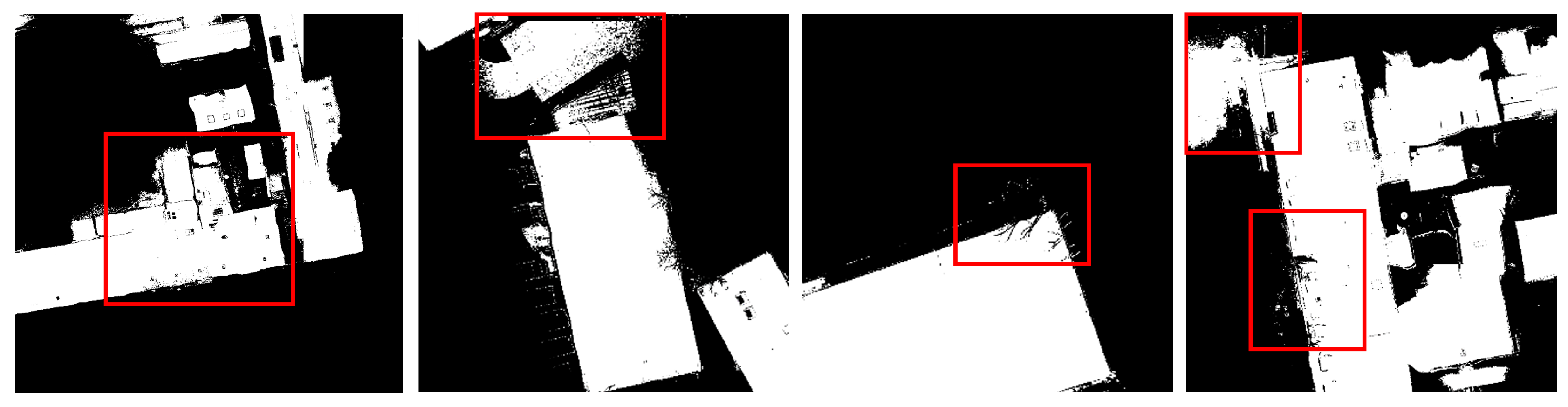
The detailed inspection in Figure 17 shows that our model incorporates salt-and-pepper noises on the model. Though the edge information provides sufficient information for reconstructing building structure, the edge information also incorporates the unwanted edge noises on the model, thereby generating salt-and-pepper noises. Several approaches have been incorporated in our model, such as applying Canny edge detector, inducing attention module for edges, or fine-tuning dense CRFs, but the excessive edge noises kept appearing. This noises may be crucial to practical applications and, thus, further studies are required to reduce noises.
5. Conclusions
In conclusion, our study introduces an innovative unsupervised framework for building segmentation. Instead of generating pseudo-labels by using low-cost labels, our framework uses SAM and spectral index-based labeling to enhance Precision in an unsupervised setting. In addition, we generated an edge-driven model that uses edge information for precise building shape reconstruction. This strategy not only prevented overfitting to pseudo-labels but also guided accurate building shape reconstruction in both unsupervised and supervised learning. Comparative analysis against state-of-the-art unsupervised segmentation models highlighted our model’s superior accuracy. Moreover, when compared with fully supervised models, our model significantly improved segmentation boundaries, designed not only for unsupervised building segmentation but also for supervised tasks, and demonstrated exceptional performance in building segmentation.
However, future research is needed to address several limitations identified in this study. Despite achieving superior results in f1-score and IoU, our model consistently tended to underestimate building segments in both unsupervised and supervised learning, leading to lower Recall despite maintaining high Precision. Inducing the edge information on the model greatly improved the performance but also made the model susceptible to noises. Furthermore, though several adjustments were made in the model to reduce edge noises through techniques like adding Gaussian noises or applying dense CRFs, the model prsesented weakness in segmenting rough roof surfaces. This constraint also contributed to a decrease in Recall, and further study is required to obtain robustness to various building roof surfaces.
Nevertheless, we established a comprehensive framework with the potential to significantly enhance unsupervised building segmentation tasks. The framework’s capacity to learn building features from inaccurate pseudo-label and edge information gives robustness to various images, and the model’s simplicity in structure makes it available to be trained in various conditions. Therefore, based on these advantages, our framework holds potential to address the lack of datasets in various aerial domains for building segmentation and also in other segmentation tasks, including land cover classification.
Author Contributions
Conceptualization, J.K.; methodology, J.K.; software, J.K.; validation, J.K.; formal analysis, J.K.; investigation, J.K.; resources, J.K.; data curation, J.K.; writing—original draft, J.K.; writing—review and editing, Y.K.; visualization, J.K.; supervision, Y.K.; project administration, Y.K.; funding acquisition, Y.K. All authors have read and agreed to the published version of the manuscript.
Funding
This work was supported by the National Research Foundation of Korea (NRF) grant funded by the Korea government (MSIT) (NRF-2023R1A2C2005548). This work was supported by the Korea Agency for Infrastructure Technology Advancement (KAIA) grant funded by the Ministry of Land, Infrastructure and Transport (Grant RS-2022-00155763). This work was also supported by the BK21 FOUR research program of the National Research Foundation of Korea.
Data Availability Statement
Data are contained within the article.
Acknowledgments
This work was financially supported by Korea Ministry of Land, Infrastructure and Transport (MOLIT) as Innovative Talent Education Program for Smart City. The Institute of Engineering Research at Seoul National University provided research facilities for work.
Conflicts of Interest
The authors declare no conflicts of interest.
References
- Mayer, H. Automatic object extraction from aerial imagery—A survey focusing on buildings. Comput. Vis. Image Underst. 1999, 74, 138–149. [Google Scholar] [CrossRef]
- Ahmadi, S.; Zoej, M.V.; Ebadi, H.; Moghaddam, H.A.; Mohammadzadeh, A. Automatic urban building boundary extraction from high resolution aerial images using an innovative model of active contours. Int. J. Appl. Earth Obs. Geoinf. 2010, 12, 150–157. [Google Scholar] [CrossRef]
- Rottensteiner, F.; Sohn, G.; Gerke, M.; Wegner, J.D. ISPRS Semantic Labeling Contest; ISPRS: Leopoldshöhe, Germany, 2014; Volume 1. [Google Scholar]
- Wang, J.; Zheng, Z.; Ma, A.; Lu, X.; Zhong, Y. LoveDA: A remote sensing land-cover dataset for domain adaptive semantic segmentation. arXiv 2021, arXiv:2110.08733. [Google Scholar]
- Van Etten, A.; Lindenbaum, D.; Bacastow, T.M. Spacenet: A remote sensing dataset and challenge series. arXiv 2018, arXiv:1807.01232. [Google Scholar]
- Ronneberger, O.; Fischer, P.; Brox, T. U-net: Convolutional networks for biomedical image segmentation. In Proceedings of the Medical Image Computing and Computer-Assisted Intervention–MICCAI 2015: 18th International Conference, Munich, Germany, 5–9 October 2015; Proceedings, Part III 18. Springer: Berlin/Heidelberg, Germany, 2015; pp. 234–241. [Google Scholar]
- Lin, T.Y.; Dollár, P.; Girshick, R.; He, K.; Hariharan, B.; Belongie, S. Feature pyramid networks for object detection. In Proceedings of the IEEE Conference on Computer Vision and Pattern Recognition (CVPR), Honolulu, HI, USA, 21–26 July 2017; pp. 2117–2125. [Google Scholar]
- Chen, L.C.; Papandreou, G.; Schroff, F.; Adam, H. Rethinking atrous convolution for semantic image segmentation. arXiv 2017, arXiv:1706.05587. [Google Scholar]
- Wang, L.; Li, R.; Zhang, C.; Fang, S.; Duan, C.; Meng, X.; Atkinson, P.M. UNetFormer: A UNet-like transformer for efficient semantic segmentation of remote sensing urban scene imagery. ISPRS J. Photogramm. Remote Sens. 2022, 190, 196–214. [Google Scholar] [CrossRef]
- Wang, L.; Li, R.; Wang, D.; Duan, C.; Wang, T.; Meng, X. Transformer meets convolution: A bilateral awareness network for semantic segmentation of very fine resolution urban scene images. Remote Sens. 2021, 13, 3065. [Google Scholar] [CrossRef]
- Dosovitskiy, A.; Beyer, L.; Kolesnikov, A.; Weissenborn, D.; Zhai, X.; Unterthiner, T.; Dehghani, M.; Minderer, M.; Heigold, G.; Gelly, S.; et al. An image is worth 16 × 16 words: Transformers for image recognition at scale. arXiv 2020, arXiv:2010.11929. [Google Scholar]
- Liu, Z.; Lin, Y.; Cao, Y.; Hu, H.; Wei, Y.; Zhang, Z.; Lin, S.; Guo, B. Swin transformer: Hierarchical vision transformer using shifted windows. In Proceedings of the IEEE/CVF International Conference on Computer Vision (ICCV), Montreal, BC, Canada, 11–17 October 2021; pp. 10012–10022. [Google Scholar]
- Foody, G.M. Status of land cover classification accuracy assessment. Remote Sens. Environ. 2002, 80, 185–201. [Google Scholar] [CrossRef]
- Jin, H.; Stehman, S.V.; Mountrakis, G. Assessing the impact of training sample selection on accuracy of an urban classification: A case study in Denver, Colorado. Int. J. Remote Sens. 2014, 35, 2067–2081. [Google Scholar] [CrossRef]
- Ji, X.; Henriques, J.F.; Vedaldi, A. Invariant information clustering for unsupervised image classification and segmentation. In Proceedings of the IEEE/CVF International Conference on Computer Vision (ICCV), Seoul, Republic of Korea, 27 October–2 November 2019; pp. 9865–9874. [Google Scholar]
- Hamilton, M.; Zhang, Z.; Hariharan, B.; Snavely, N.; Freeman, W.T. Unsupervised semantic segmentation by distilling feature correspondences. arXiv 2022, arXiv:2203.08414. [Google Scholar]
- Seong, H.S.; Moon, W.; Lee, S.; Heo, J.P. Leveraging Hidden Positives for Unsupervised Semantic Segmentation. In Proceedings of the IEEE/CVF Conference on Computer Vision and Pattern Recognition (CVPR), Vancouver, BC, Canada, 17–24 June 2023; pp. 19540–19549. [Google Scholar]
- Caron, M.; Touvron, H.; Misra, I.; Jégou, H.; Mairal, J.; Bojanowski, P.; Joulin, A. Emerging properties in self-supervised vision transformers. In Proceedings of the IEEE/CVF International Conference on Computer Vision (ICCV), Montreal, BC, Canada, 11–17 October 2021; pp. 9650–9660. [Google Scholar]
- Shen, W.; Peng, Z.; Wang, X.; Wang, H.; Cen, J.; Jiang, D.; Xie, L.; Yang, X.; Tian, Q. A survey on label-efficient deep image segmentation: Bridging the gap between weak supervision and dense prediction. IEEE Trans. Pattern Anal. Mach. Intell. 2023, 45, 9284–9305. [Google Scholar] [CrossRef]
- Lee, D.H. Pseudo-label: The simple and efficient semi-supervised learning method for deep neural networks. In Proceedings of the Workshop on Challenges in Representation Learning, ICML, Atlanta, GA, USA, 16–21 June 2013; Volume 3, p. 896. [Google Scholar]
- Li, Z.; Zhang, X.; Xiao, P.; Zheng, Z. On the effectiveness of weakly supervised semantic segmentation for building extraction from high-resolution remote sensing imagery. IEEE J. Sel. Top. Appl. Earth Obs. Remote Sens. 2021, 14, 3266–3281. [Google Scholar] [CrossRef]
- Vernaza, P.; Chandraker, M. Learning random-walk label propagation for weakly-supervised semantic segmentation. In Proceedings of the IEEE Conference on Computer Vision and Pattern Recognition (CVPR), Honolulu, HI, USA, 21–26 July 2017; pp. 7158–7166. [Google Scholar]
- Wang, S.; Chen, W.; Xie, S.M.; Azzari, G.; Lobell, D.B. Weakly supervised deep learning for segmentation of remote sensing imagery. Remote Sens. 2020, 12, 207. [Google Scholar] [CrossRef]
- Song, C.; Huang, Y.; Ouyang, W.; Wang, L. Box-driven class-wise region masking and filling rate guided loss for weakly supervised semantic segmentation. In Proceedings of the IEEE/CVF Conference on Computer Vision and Pattern Recognition (CVPR), Long Beach, CA, USA, 15–20 June 2019; pp. 3136–3145. [Google Scholar]
- Cheng, T.; Wang, X.; Chen, S.; Zhang, Q.; Liu, W. Boxteacher: Exploring high-quality pseudo labels for weakly supervised instance segmentation. In Proceedings of the IEEE/CVF Conference on Computer Vision and Pattern Recognition (CVPR), Vancouver, BC, Canada, 17–24 June 2023; pp. 3145–3154. [Google Scholar]
- Chen, H.; Cheng, L.; Zhuang, Q.; Zhang, K.; Li, N.; Liu, L.; Duan, Z. Structure-aware weakly supervised network for building extraction from remote sensing images. IEEE Trans. Geosci. Remote Sens. 2022, 60, 1–12. [Google Scholar] [CrossRef]
- Xu, L.; Clausi, D.A.; Li, F.; Wong, A. Weakly supervised classification of remotely sensed imagery using label constraint and edge penalty. IEEE Trans. Geosci. Remote Sens. 2016, 55, 1424–1436. [Google Scholar] [CrossRef]
- Zhou, B.; Khosla, A.; Lapedriza, A.; Oliva, A.; Torralba, A. Learning deep features for discriminative localization. In Proceedings of the IEEE Conference on Computer Vision and Pattern Recognition (CVPR), Las Vegas, NV, USA, 1–26 July 2016; pp. 2921–2929. [Google Scholar]
- Obukhov, A.; Georgoulis, S.; Dai, D.; Van Gool, L. Gated CRF loss for weakly supervised semantic image segmentation. arXiv 2019, arXiv:1906.04651. [Google Scholar]
- Zhang, J.; Yu, X.; Li, A.; Song, P.; Liu, B.; Dai, Y. Weakly-supervised salient object detection via scribble annotations. In Proceedings of the IEEE/CVF Conference on Computer Vision and Pattern Recognition (CVPR), Seattle, WA, USA, 13–19 June 2020; pp. 12546–12555. [Google Scholar]
- Lee, S.; Lee, M.; Lee, J.; Shim, H. Railroad is not a train: Saliency as pseudo-pixel supervision for weakly supervised semantic segmentation. In Proceedings of the IEEE/CVF Conference on Computer Vision and Pattern Recognition (CVPR), Nashville, TN, USA, 20–25 June 2021; pp. 5495–5505. [Google Scholar]
- Kirillov, A.; Mintun, E.; Ravi, N.; Mao, H.; Rolland, C.; Gustafson, L.; Xiao, T.; Whitehead, S.; Berg, A.C.; Lo, W.Y.; et al. Segment anything. arXiv 2023, arXiv:2304.02643. [Google Scholar]
- Ren, S.; Luzi, F.; Lahrichi, S.; Kassaw, K.; Collins, L.M.; Bradbury, K.; Malof, J.M. Segment anything, from space? arXiv 2023, arXiv:2304.13000. [Google Scholar]
- Bradbury, K.; Saboo, R.; L Johnson, T.; Malof, J.M.; Devarajan, A.; Zhang, W.; M Collins, L.; G Newell, R. Distributed solar photovoltaic array location and extent dataset for remote sensing object identification. Sci. Data 2016, 3, 160106. [Google Scholar] [CrossRef]
- Maggiori, E.; Tarabalka, Y.; Charpiat, G.; Alliez, P. Can semantic labeling methods generalize to any city? The inria aerial image labeling benchmark. In Proceedings of the 2017 IEEE International Geoscience and Remote Sensing Symposium (IGARSS), Fort Worth, TX, USA, 23–28 July 2017; pp. 3226–3229. [Google Scholar]
- Demir, I.; Koperski, K.; Lindenbaum, D.; Pang, G.; Huang, J.; Basu, S.; Hughes, F.; Tuia, D.; Raskar, R. Deepglobe 2018: A challenge to parse the earth through satellite images. In Proceedings of the IEEE Conference on Computer Vision and Pattern Recognition Workshops (CVPRW), Salt Lake City, UT, USA, 18–22 June 2018; pp. 172–181. [Google Scholar]
- Mohajerani, S.; Saeedi, P. Cloud-Net: An end-to-end cloud detection algorithm for Landsat 8 imagery. In Proceedings of the 2019 IEEE International Geoscience and Remote Sensing Symposium (IGARSS), Yokohama, Japan, 28 July–2 August 2019; pp. 1029–1032. [Google Scholar]
- Aung, H.L.; Uzkent, B.; Burke, M.; Lobell, D.; Ermon, S. Farm parcel delineation using spatio-temporal convolutional networks. In Proceedings of the IEEE/CVF Conference on Computer Vision and Pattern Recognition Workshops (CVPRW), Seattle, WA, USA, 14–19 June 2020; pp. 76–77. [Google Scholar]
- Canny, J. A computational approach to edge detection. IEEE Trans. Pattern Anal. Mach. Intell. 1986, PAMI-8, 679–698. [Google Scholar] [CrossRef]
- Krähenbühl, P.; Koltun, V. Efficient inference in fully connected crfs with gaussian edge potentials. Adv. Neural Inf. Process. Syst. 2011, 24, 109–117. [Google Scholar]
- Thenkabail, P.S. Remotely Sensed Data Characterization, Classification, and Accuracies; CRC Press: Boca Raton, FL, USA, 2015; Volume 1, p. 7. [Google Scholar]
- Cheng, H.D.; Jiang, X.H.; Sun, Y.; Wang, J. Color image segmentation: Advances and prospects. Pattern Recognit. 2001, 34, 2259–2281. [Google Scholar] [CrossRef]
- Xiao, C.; Qin, R.; Huang, X. Treetop detection using convolutional neural networks trained through automatically generated pseudo labels. Int. J. Remote Sens. 2020, 41, 3010–3030. [Google Scholar] [CrossRef]
- Mhangara, P.; Odindi, J.; Kleyn, L.; Remas, H. Road Extraction Using Object Oriented Classification. Vis. Tech. Available online: https://www.researchgate.net/profile/John-Odindi/publication/267856733_Road_extraction_using_object_oriented_classification/links/55b9fec108aed621de09550a/Road-extraction-using-object-oriented-classification.pdf (accessed on 5 December 2023).
- Ma, X.; Li, B.; Zhang, Y.; Yan, M. The Canny Edge Detection and Its Improvement. In Proceedings of the Artificial Intelligence and Computational Intelligence, Chengdu, China, 26–28 October 2012; Lei, J., Wang, F.L., Deng, H., Miao, D., Eds.; Springer: Berlin/Heidelberg, Germnay, 2012; pp. 50–58. [Google Scholar]
- Woo, S.; Park, J.; Lee, J.Y.; Kweon, I.S. Cbam: Convolutional block attention module. In Proceedings of the European Conference on Computer Vision (ECCV), Munich, Germany, 8–14 September 2018; pp. 3–19. [Google Scholar]
- Kingma, D.P.; Ba, J. Adam: A method for stochastic optimization. arXiv 2014, arXiv:1412.6980. [Google Scholar]
- He, K.; Zhang, X.; Ren, S.; Sun, J. Delving deep into rectifiers: Surpassing human-level performance on imagenet classification. In Proceedings of the IEEE International Conference on Computer Vision, Santiago, Chile, 7–13 December 2015; pp. 1026–1034. [Google Scholar]
- Zhang, Z.; Liu, Q.; Wang, Y. Road extraction by deep residual u-net. IEEE Geosci. Remote Sens. Lett. 2018, 15, 749–753. [Google Scholar] [CrossRef]
- Li, R.; Zheng, S.; Zhang, C.; Duan, C.; Su, J.; Wang, L.; Atkinson, P.M. Multiattention Network for Semantic Segmentation of Fine-Resolution Remote Sensing Images. IEEE Trans. Geosci. Remote Sens. 2022, 60, 1–13. [Google Scholar] [CrossRef]
- Zhou, T.; Fu, H.; Sun, C.; Wang, S. Shadow detection and compensation from remote sensing images under complex urban conditions. Remote Sens. 2021, 13, 699. [Google Scholar] [CrossRef]
Figure 1.
Flowchart of the entire unsupervised building segmentation framework.

Figure 2.
Structure of SAM with a point prompt and corresponding mask.

Figure 3.
Sequential masking of polygons: (a) Original image, (b) Initial SAM masks generated on auto-prompt mode, (c) The result after applying area-based threshold, (d) The result after applying NDVI and BAI-based threshold.
Figure 3.
Sequential masking of polygons: (a) Original image, (b) Initial SAM masks generated on auto-prompt mode, (c) The result after applying area-based threshold, (d) The result after applying NDVI and BAI-based threshold.

Figure 4.
The results after unsupervised feature extraction: (a) Original image, (b) The result after applying Canny edge detector, (c) Ground-truth for comparison, (d) Generated pseudo-label.
Figure 4.
The results after unsupervised feature extraction: (a) Original image, (b) The result after applying Canny edge detector, (c) Ground-truth for comparison, (d) Generated pseudo-label.

Figure 5.
The structure of our proposed edge-driven model.

Figure 6.
Structure of CBAM.

Figure 7.
The fine-tuning of CRFs. The red box represents the best result.

Figure 8.
ISPRS Potsdam dataset. (a) Original Image, (b) Original 6-class Potsdam label, (c) Extracted Potsdam building label.
Figure 8.
ISPRS Potsdam dataset. (a) Original Image, (b) Original 6-class Potsdam label, (c) Extracted Potsdam building label.

Figure 9.
Loss values using the unsupervised method.

Figure 10.
The result for unsupervised models on Potsdam dataset, each image represents: (a) Original Image, (b) IIC, (c) STEGO, (d) HP, (e) Pseudo-Label, (f) Proposed Method, (g) Ground-Truth.
Figure 10.
The result for unsupervised models on Potsdam dataset, each image represents: (a) Original Image, (b) IIC, (c) STEGO, (d) HP, (e) Pseudo-Label, (f) Proposed Method, (g) Ground-Truth.

Figure 11.
The result for unsupervised models on Vaihingen dataset, each image represents: (a) Original Image, (b) IIC, (c) STEGO, (d) HP, (e) Pseudo-Label, (f) Proposed Method, (g) Ground-Truth.
Figure 11.
The result for unsupervised models on Vaihingen dataset, each image represents: (a) Original Image, (b) IIC, (c) STEGO, (d) HP, (e) Pseudo-Label, (f) Proposed Method, (g) Ground-Truth.

Figure 12.
The result for unsupervised models on full Potsdam images; each image represents (a) Original Image, (b) IIC, (c) STEGO, (d) HP, (e) Pseudo-Label, (f) Proposed Method, (g) Ground-Truth.
Figure 12.
The result for unsupervised models on full Potsdam images; each image represents (a) Original Image, (b) IIC, (c) STEGO, (d) HP, (e) Pseudo-Label, (f) Proposed Method, (g) Ground-Truth.

Figure 13.
The result for supervised models on Potsdam: (a) Original image, (b) U-Net, (c) ResUNet, (d) DeepLabV3+, (e) MANet, (f) Proposed Method, (g) Ground-Truth.
Figure 13.
The result for supervised models on Potsdam: (a) Original image, (b) U-Net, (c) ResUNet, (d) DeepLabV3+, (e) MANet, (f) Proposed Method, (g) Ground-Truth.

Figure 14.
The result for supervised models on Vaihingen: (a) Original image, (b) U-Net, (c) ResUNet, (d) DeepLabV3+, (e) MANet, (f) Proposed Method, (g) Ground-Truth.
Figure 14.
The result for supervised models on Vaihingen: (a) Original image, (b) U-Net, (c) ResUNet, (d) DeepLabV3+, (e) MANet, (f) Proposed Method, (g) Ground-Truth.

Figure 15.
The evaluation metrics on weight . The center line exhibits the metrics with zero weight.
Figure 15.
The evaluation metrics on weight . The center line exhibits the metrics with zero weight.

Figure 16.
The result for building (red), vegetation (green), and road (blue): (a) Original Image, (b) IIC, (c) STEGO, (d) HP, (e) Pseudo-label with NDVI and BAI, (f) Proposed Method, (g) Ground-Truth.
Figure 16.
The result for building (red), vegetation (green), and road (blue): (a) Original Image, (b) IIC, (c) STEGO, (d) HP, (e) Pseudo-label with NDVI and BAI, (f) Proposed Method, (g) Ground-Truth.

Figure 17.
Detected salt-and-pepper noises in an unsupervised method.


Table 1.
Comparison of unsupervised models on Potsdam.
| Dataset | Models | f1-Score | Precision | Recall | IoU |
|---|---|---|---|---|---|
| Potsdam | IIC | 0.4587 | 0.4315 | 0.5110 | 0.3013 |
| STEGO | 0.7557 | 0.7775 | 0.7408 | 0.6122 | |
| HP | 0.7771 | 0.8063 | 0.7532 | 0.6390 | |
| Pseudo-Label | 0.7363 | 0.7273 | 0.7548 | 0.5850 | |
| Proposed Method | 0.7829 | 0.8569 | 0.7231 | 0.6463 |
Table 2.
Comparison of unsupervised models on Vaihingen.
| Dataset | Models | f1-Score | Precision | Recall | IoU |
|---|---|---|---|---|---|
| Vaihingen | IIC | 0.4042 | 0.3793 | 0.4422 | 0.2618 |
| STEGO | 0.7330 | 0.7068 | 0.7613 | 0.5741 | |
| HP | 0.7567 | 0.7709 | 0.7430 | 0.6226 | |
| Pseudo-Label | 0.7108 | 0.7066 | 0.7156 | 0.5504 | |
| Proposed Method | 0.7779 | 0.8242 | 0.7483 | 0.6453 |
Table 3.
Comparison of supervised models on Potsdam.
| Methods | Models | f1-Score | Precision | Recall | IoU |
|---|---|---|---|---|---|
| Potsdam | DeepLabV3+ | 0.8344 | 0.8371 | 0.8444 | 0.7216 |
| ResUNet | 0.8504 | 0.8687 | 0.8381 | 0.7427 | |
| U-Net | 0.8228 | 0.8333 | 0.8363 | 0.7088 | |
| MANet | 0.8540 | 0.8601 | 0.8536 | 0.7481 | |
| Proposed Method | 0.8512 | 0.9072 | 0.8080 | 0.7442 |
Table 4.
Comparison of supervised models on Vaihingen.
| Methods | Models | f1-Score | Precision | Recall | IoU |
|---|---|---|---|---|---|
| Vaihingen | DeepLabV3+ | 0.8241 | 0.8204 | 0.8487 | 0.7016 |
| ResUNet | 0.8335 | 0.8286 | 0.8381 | 0.7142 | |
| U-Net | 0.8183 | 0.8139 | 0.8357 | 0.6953 | |
| MANet | 0.8415 | 0.8257 | 0.8583 | 0.7262 | |
| Proposed Method | 0.8435 | 0.8632 | 0.8242 | 0.7295 |
Table 5.
Comparison of weight and evaluation metrics.
| Weight | ||||||||
|---|---|---|---|---|---|---|---|---|
| Metrics | 0.0 | 0.1 | 0.2 | 0.3 | 0.4 | 0.5 | 0.6 | 0.7 |
| f1-score | 0.7065 | 0.7138 | 0.7828 | 0.7641 | 0.7186 | 0.6714 | 0.6998 | 0.7055 |
| Precision | 0.8196 | 0.7057 | 0.8569 | 0.8595 | 0.6832 | 0.6169 | 0.6789 | 0.7387 |
| Recall | 0.6306 | 0.7326 | 0.7531 | 0.6922 | 0.7659 | 0.7529 | 0.7313 | 0.6863 |
| IoU | 0.5488 | 0.5583 | 0.6563 | 0.6207 | 0.5638 | 0.5099 | 0.5412 | 0.5484 |
Table 6.
Comparison of f1-score and IoU for building, vegetation, and road.
| f1-Score | IoU | ||||||
|---|---|---|---|---|---|---|---|
| Methods | Models | Bldg. | Veg. | Road. | Bldg. | Veg. | Road. |
| Unsupervised | IIC | 0.4587 | 0.8237 | 0.5789 | 0.3013 | 0.7021 | 0.4112 |
| STEGO | 0.7557 | 0.8007 | 0.7144 | 0.6122 | 0.6759 | 0.5570 | |
| HP | 0.7771 | 0.8461 | 0.7928 | 0.6390 | 0.7030 | 0.6578 | |
| Pseudo-Label | 0.7363 | 0.7762 | 0.6640 | 0.5850 | 0.6455 | 0.5012 | |
| Proposed Method | 0.7829 | 0.8108 | 0.7222 | 0.6464 | 0.6887 | 0.5677 | |
Table 7.
Comparison of model parameters.
| Methods | Models | Parameter | Trainable | Running Time (h) | Inference Time (ms) |
|---|---|---|---|---|---|
| Supervised | DeepLabV3+ | 41 M | 41 M | 0.78 | 9.81 |
| ResUNet | 31 M | 31 M | 0.85 | 17.70 | |
| U-Net | 23 M | 23 M | 0.80 | 16.19 | |
| MANet | 36 M | 36 M | 0.61 | 12.76 | |
| Unsupervised | STEGO | 49 M | 27 M | 2.36 | 41.10 |
| IIC | 4 M | 4 M | 0.48 | 22.36 | |
| HP | 87 M | 9.8 M | 1.92 | 107.13 | |
| Proposed Method | 8 M | 8 M | 0.52 | 23.78 |
Disclaimer/Publisher’s Note: The statements, opinions and data contained in all publications are solely those of the individual author(s) and contributor(s) and not of MDPI and/or the editor(s). MDPI and/or the editor(s) disclaim responsibility for any injury to people or property resulting from any ideas, methods, instructions or products referred to in the content. |
© 2024 by the authors. Licensee MDPI, Basel, Switzerland. This article is an open access article distributed under the terms and conditions of the Creative Commons Attribution (CC BY) license (https://creativecommons.org/licenses/by/4.0/).
Share and Cite
MDPI and ACS Style
Kim, J.; Kim, Y. Integrated Framework for Unsupervised Building Segmentation with Segment Anything Model-Based Pseudo-Labeling and Weakly Supervised Learning. Remote Sens. 2024, 16, 526. https://doi.org/10.3390/rs16030526
AMA Style
Kim J, Kim Y. Integrated Framework for Unsupervised Building Segmentation with Segment Anything Model-Based Pseudo-Labeling and Weakly Supervised Learning. Remote Sensing. 2024; 16(3):526. https://doi.org/10.3390/rs16030526
Chicago/Turabian StyleKim, Jiyong, and Yongil Kim. 2024. "Integrated Framework for Unsupervised Building Segmentation with Segment Anything Model-Based Pseudo-Labeling and Weakly Supervised Learning" Remote Sensing 16, no. 3: 526. https://doi.org/10.3390/rs16030526
Note that from the first issue of 2016, this journal uses article numbers instead of page numbers. See further details here.