


Sea Ice Detection from RADARSAT-2 Quad-Polarization SAR Imagery Based on Co- and Cross-Polarization Ratio

1
School of Marine Sciences, Nanjing University of Information Science and Technology, Nanjing 210044, China
2
Laboratory for Regional Oceanography and Numerical Modeling, Qingdao National Laboratory for Marine Science and Technology, Qingdao 266237, China
3
School of Remote Sensing and Geomatics Engineering, Nanjing University of Information Science and Technology, Nanjing 210044, China
4
Department of Fisheries and Oceans Canada, Bedford Institute of Oceanography, Dartmouth, NS B2Y 4A2, Canada
5
State Key Laboratory of Satellite Ocean Environment Dynamics, Second Institute of Oceanography, Ministry of Natural Resources, Hangzhou 310012, China
*
Author to whom correspondence should be addressed.
Remote Sens. 2024, 16(3), 515; https://doi.org/10.3390/rs16030515
Submission received: 11 December 2023
/
Revised: 23 January 2024
/
Accepted: 26 January 2024
/
Published: 29 January 2024
(This article belongs to the Special Issue Recent Advances in Sea Ice Research Using Satellite Data)
Abstract
:Arctic sea ice detection is very important in global climate research, Arctic ecosystem protection, ship navigation and human activities. In this paper, by combining the co-pol ratio (HH/VV) and two kinds of cross-pol ratio (HV/VV, HV/HH), a novel sea ice detection method is proposed based on RADARSAT-2 quad-polarization synthetic aperture radar (SAR) images. Experimental results suggest that the co-pol ratio shows promising capability in sea ice detection at a wide range of incidence angles (25–50°), while the two kinds of cross-pol ratio are more applicable to sea ice detection at small incidence angles (20–35°). When incidence angles exceed 35°, wind conditions have a great effect on the performance of the cross-pol ratio. Our method is validated by comparison with the visual interpretation results. The overall accuracy is 96%, far higher than that of single polarization ratio (PR) parameter-based methods. Our method is suitable for sea ice detection in complex sea ice and wind conditions.

1. Introduction
As an important component of the Arctic, sea ice plays an essential role in Arctic climate and ecosystems. Changes in Arctic sea ice have significant effects on global temperature, ocean currents and biodiversity [1,2,3]. Long time-series satellite observations and climate model predictions have demonstrated a decrease in sea ice cover and thickness [4,5,6,7,8], due to global warming caused by emissions of massive amounts of greenhouse gases. An examination of nearly four decades of pan-Arctic sea ice drift data obtained from satellite sensors indicates a general rise in the intensity of ocean currents in the Beaufort Gyre and Transpolar Drift [9]. This notable upward trend in ice drift speeds, amounting to approximately 20% per decade, cannot be attributed to the comparatively weaker trend in wind speeds. Rather, it is linked to the substantial trend in regions experiencing multiyear ice depletion and exhibiting relatively low ice concentrations. Due to the reduction in sea ice, sea-ice fauna, endemic fish and megafauna are experiencing a decline. However, the phytoplankton biomass may increase due to increasing light penetration [2].
Significant changes have been observed in the Arctic climate. A recent study suggests that Arctic temperatures are increasing four times faster than global warming [10]. Moreover, some abnormal weather events have occurred in the Arctic region [11,12], such as abnormal heat, fires, increased rainfall, etc. These events have had a significant impact on the local environment, ecosystems, economies and communities. Furthermore, the accelerating sea ice melting is driving an increase in Arctic activities, such as fishing, tourism and shipping through the Northeast Passage between the Atlantic and Pacific Oceans. From the viewpoint of both navigation security and efficiency, this leads to the urgent demand to provide near-real-time sea ice detection maps in support of these activities.
In recent decades, Arctic countries, such as Canada, America, Russia and Norway, have been continuing to provide daily or weekly sea ice charts based on manual visual interpretation of multisource satellite imagery. Synthetic aperture radar (SAR) images are more often used to produce sea ice charts due to their high resolution, wide coverage and the capability of working day and night. Other observation data from passive microwave radiometer (MWR) and optical sensors will also be analyzed by ice experts to provide complementary sea ice information if they are available. Because the albedo of sea ice is much higher than that of open water (OW), it is quite easy to discriminate bright sea ice from dark OW in optical imagery. However, its strong dependence on sun illumination and cloud-free weather conditions restricts its use in practical sea ice charting. The MWR data have been widely used for producing operational global sea ice concentration (SIC) products based on a series of mature retrieval algorithms [13,14,15,16,17,18,19], but their coarse resolution (in the order of tens of kilometers) cannot meet the practical demands of society, such as Arctic navigation.
The backscattering signatures of OW and different sea ice conditions are quite complex in SAR images. Moreover, they easily become ambiguous in high wind conditions. In particular, various sea ice types and OW can have very close backscatter signatures. Therefore, professional knowledge is needed to produce high-quality sea ice detection products. In addition, it is labor-intensive and time-consuming for ice experts to interpret a large amount of SAR images. Specifically, it usually takes 6–12 h or more time to deliver sea ice maps to users, which reduces their value, especially in the rapidly changing marginal ice zone (MIZ). Generating high-resolution sea ice maps from SAR imagery using automatic methodologies can significantly shorten this process, and thus make better use of their value.
A series of SAR-based sea ice detection methods have been proposed in the past thirty years, such as feature-based machine learning (ML) methods and deep learning (DL) methods. Typical ML methods consist of a two-stage process. First, various polarimetric and texture features are derived from SAR images [20,21]. Specific polarimetric features include normalized radar cross section (NRCS), polarization ratio (PR), phase difference, correlation coefficient and parameters calculated based on eigenvalue decomposition, Pauli decomposition or Freeman–Durden decomposition methods [22,23,24,25]. Gray-level co-occurrence matrices (GLCMs) are the most popular methods for texture feature extraction [24,26,27,28,29]. After feature extraction, a ML model is then employed to classify sea ice, such as random forest (RF) [29,30], k-means [22,24], supporting vector machine (SVM) [26,27,28,31,32,33,34], decision tree [23] and Bayesian methods [35]. The main drawback of these methodologies is that the complicated feature engineering methodologies require a high level of professional knowledge and a large amount of time to pick up the optimal features. DL methods can deal with this challenge. Convolutional neural networks (CNNs) have been widely used in SAR-based sea ice detection, and have shown promising results [36,37,38,39,40,41,42,43,44]. The main disadvantage of DL methods is the lack of explanation of the physical mechanisms. Consequently, DL methods may sometimes experience robustness and generalization issues.
The PR method, defined as the ratio of two polarization channels, is related to radar parameters (center frequency, incidence angles), physical characteristics of sea ice and OW (salinity, relative dielectric constant, surface roughness, etc.) and environmental conditions such as wind conditions. Because of the large PR difference between sea ice and OW, the PR method has been employed in numerous previous research studies to distinguish between sea ice and OW [22,23,24,45,46]. For instance, Geldsetzer and Yackel utilized a decision-tree classifier to differentiate sea ice and OW based on twenty ENVISAT ASAR dual co-polarized medium-resolution images [23]. They determined that the classification accuracy for OW is 50% when employing a co-pol ratio (VV/HH) threshold of 2 dB. The discrimination between multiyear ice and smooth first year ice was found to be more than 99% accurate. However, 50% of the pixels were misclassified as thin ice. They also found that the co-pol ratio threshold cannot be used to detect sea ice and OW at small incidence angles because of the relatively small co-pol ratio difference between sea ice and OW. Gill and Yackel evaluated the potential of polarimetric parameters for classifying three ice types and OW based on nine RADARSAT-2 quad-pol SAR images [22]. A single-parameter supervised k-means classification was conducted on an image obtained on 4 May 2008, with an incidence angle of 27°. The overall classification accuracy of the co-pol ratio (HH/VV) and cross-pol ratio (HH/HV) was 43.83% and 42.92%, respectively. Although they also analyzed the classification potential of two-parameter and three-parameter combinations, the combination of co-pol ratio and cross-pol ratio was not included in the evaluation. Xie et al. proposed a theoretical co-pol ratio (VV/HH) model based on an X-Bragg model [47]. The theoretical co-pol ratio model was built as a function of incidence angles, dielectric constant, orientation angle shift and its standard deviation. Hence, the backscatter of the ocean surface could be distinguished as either OW or sea ice through a comparison of the measured co-pol ratio with a theoretical model for the co-pol ratio. Six RADARSAT-2 quad-pol SAR images with incidence angles ranging from 28.10° to 49.50 were used to validate the algorithm. The overall accuracy was 96%.
Based on the above analysis, we found that there are several limitations in these studies. Firstly, the small datasets are not large enough to produce convincing statistical results. Secondly, since the PR is associated with incidence angles and wind conditions, the dataset should include a wide range of incidence angles and wind conditions. Lastly, the classification potential of a combination of co-pol ratio and cross-pol ratio needs to be investigated in sea ice detection based on quad-pol SAR images.
To solve these limitations, in this paper a total of 131 RADARSAT-2 quad-pol SAR images are used to study the characteristics of co-pol and cross-pol ratio with respect to a wide range of incidence angles and wind conditions. Then, an automatic sea ice detection algorithm has been developed based on co-pol and cross-pol ratio parameters derived from RADARSAT-2 quad-pol SAR images. By comparison to visual manual interpretations and other previous similar algorithms, our method is evaluated and validated comprehensively.
2. Materials and Methods
2.1. Study Area and Data
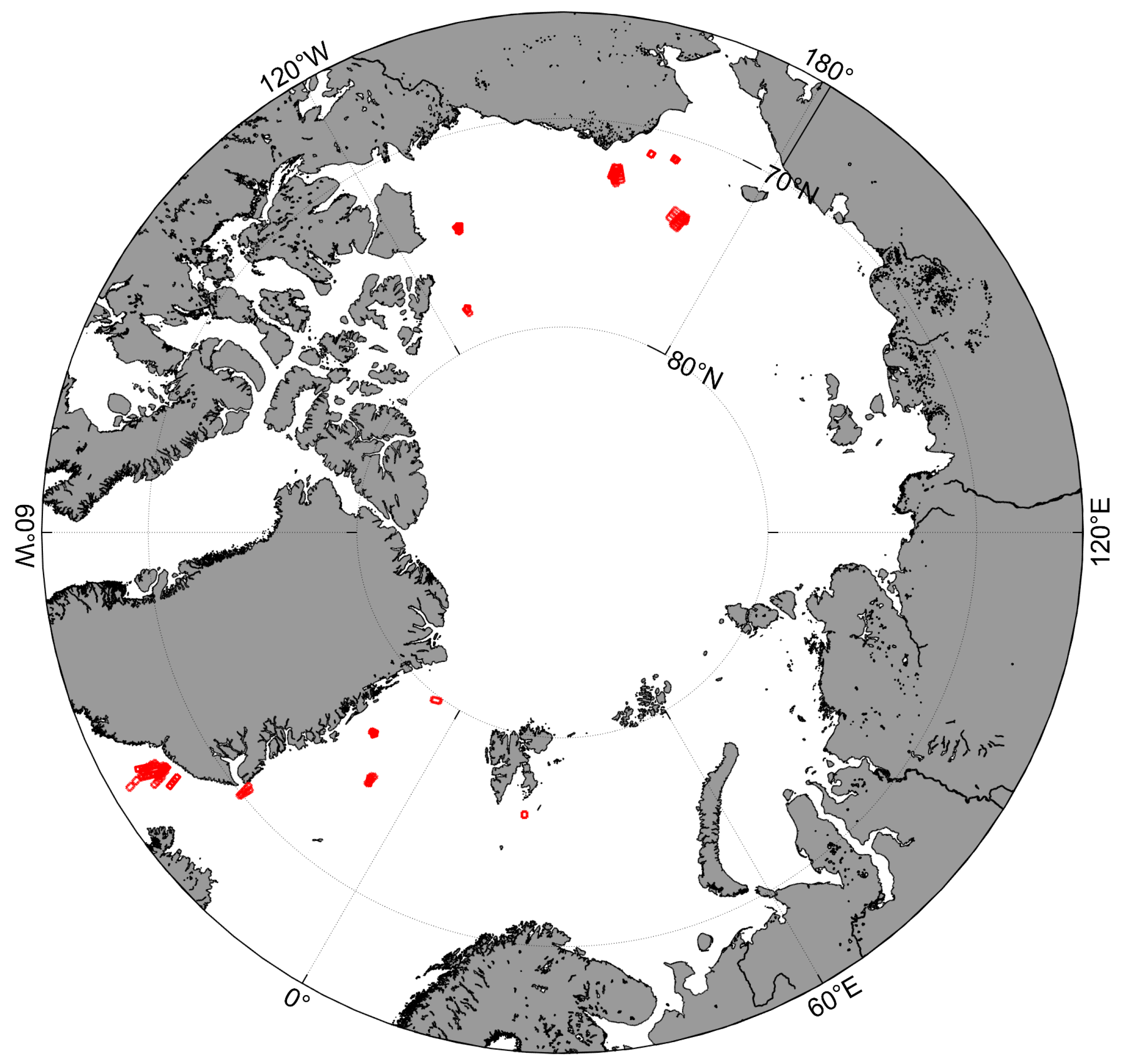
We collected 131 RADARSAT-2 fine quad-polarization (HH/VV/HV/VH) single look complex (SLC) SAR images in the MIZ of the Beaufort Sea and Chukchi Sea, and off the east coast of Greenland during 2013–2019. These images were selected to cover both OW and various sea ice types: young ice, first-year ice and multi-year ice under different wind and sea conditions (rough and calm OW). Wind conditions were derived from ECMWF (European Centre for Medium-Range Weather Forecasts) Reanalysis v5 (ERA5) datasets. The wind speed is in the range of 1.6–20.4 m/s.
The footprints of these SAR images are shown in Figure 1. Details about the RADARSAT-2 quad-polarization SAR images used in this study are given in Table 1. The fine quad-polarization mode is able to provide VV, HH, HV and HV polarized SAR images with a low noise floor (−36.5 ± 3 dB). The nominal range and azimuth resolution are 5.2 m and 7.6 m, respectively. The range of incidence angles is between 19° and 49°. The incidence angles vary by about 1.5° across a swath of 25 km.
2.2. SAR Polarimetric Parameters
The scattering matrix serves as the fundamental observation of the SAR full polarimetric mode at individual pixels. It comprises four complex elements that characterize the polarization transformation of an incident wave pulse, upon interaction with a reflective medium, to the polarization of the backscattered wave. The scattering matrix for the quad-pol mode can be written as:
where , /, are complex scattering coefficients, corresponding to horizontal polarization (HH-pol), cross polarization (HV/VH-pol) and vertical polarization (VV-pol), respectively.
Then, the normalized radar cross section (NRCS) can be calculated by multiplying the polarimetric scattering coefficients and their conjugate values, which are given as follows:
where , denote horizontal (H) or vertical (V) polarization, and is complex conjugation. indicates the ensemble averaging to reduce speckle noise. The window size for averaging is 10 × 10 pixels in this study.
The dominant scattering mechanism of OW is Bragg scattering for VV- and HH-pol, whereas the nature of scatter contributions to cross-pol is quite different. The cross-pol signals are more sensitive to local out-of-plane of incidence tilting effects [48]. For sea ice, VV- and HH-pol are typically related to the surface scattering, while the cross-pol mainly provides information about volume scattering.
The PR parameters can be derived from the scattering matrix directly. The co-pol ratio is defined as:
Two kinds of cross-pol ratio are defined as follows:
The co-pol ratio and cross-pol ratio of sea ice and OW have different responses to incidence angle effects, and therefore can be used to discriminate sea ice and OW. In this paper, an automatic sea ice detection algorithm is developed based on the combination of the co-pol and cross-pol ratios.
2.3. Sea Ice Detection Method Based on PR
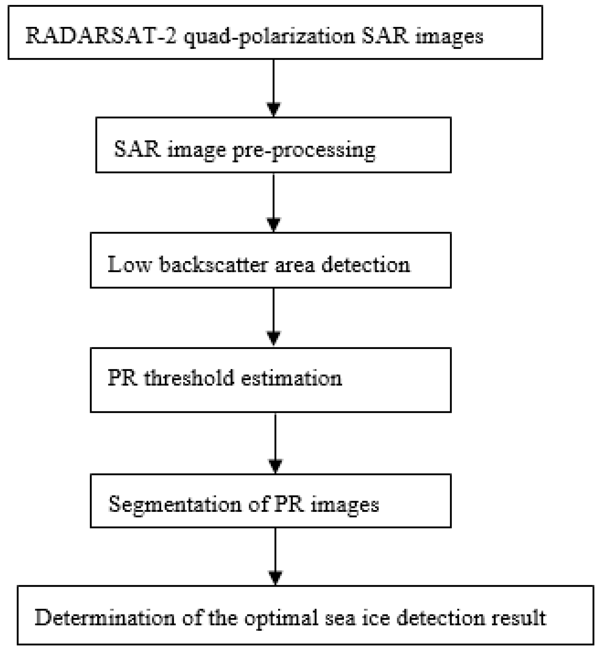
The flow chart for our sea ice detection algorithm is given in Figure 2.
The key processing steps include:
- (1)
- SAR image pre-processing:
To obtain the NRCS in HH, VV-, HV- and VH-pol, radiometric calibration is performed for all quad-polarization SAR images by using the following formula:
where is the complex scattering coefficient in the scattering matrix, and is the gain value recorded in the ‘lutSigma.xml’ file.
Then, the 3 × 3 Lee filter [49] and a boxcar averaging operation is applied to reduce speckle noise and smooth the image to 50-m pixel spacing. After that, the co-pol ratio and two kinds of cross-pol ratio are calculated according to Equations (3)–(5). The NRCS and PR are converted to dB units by convention.
- (2)
- Low backscatter area detection:
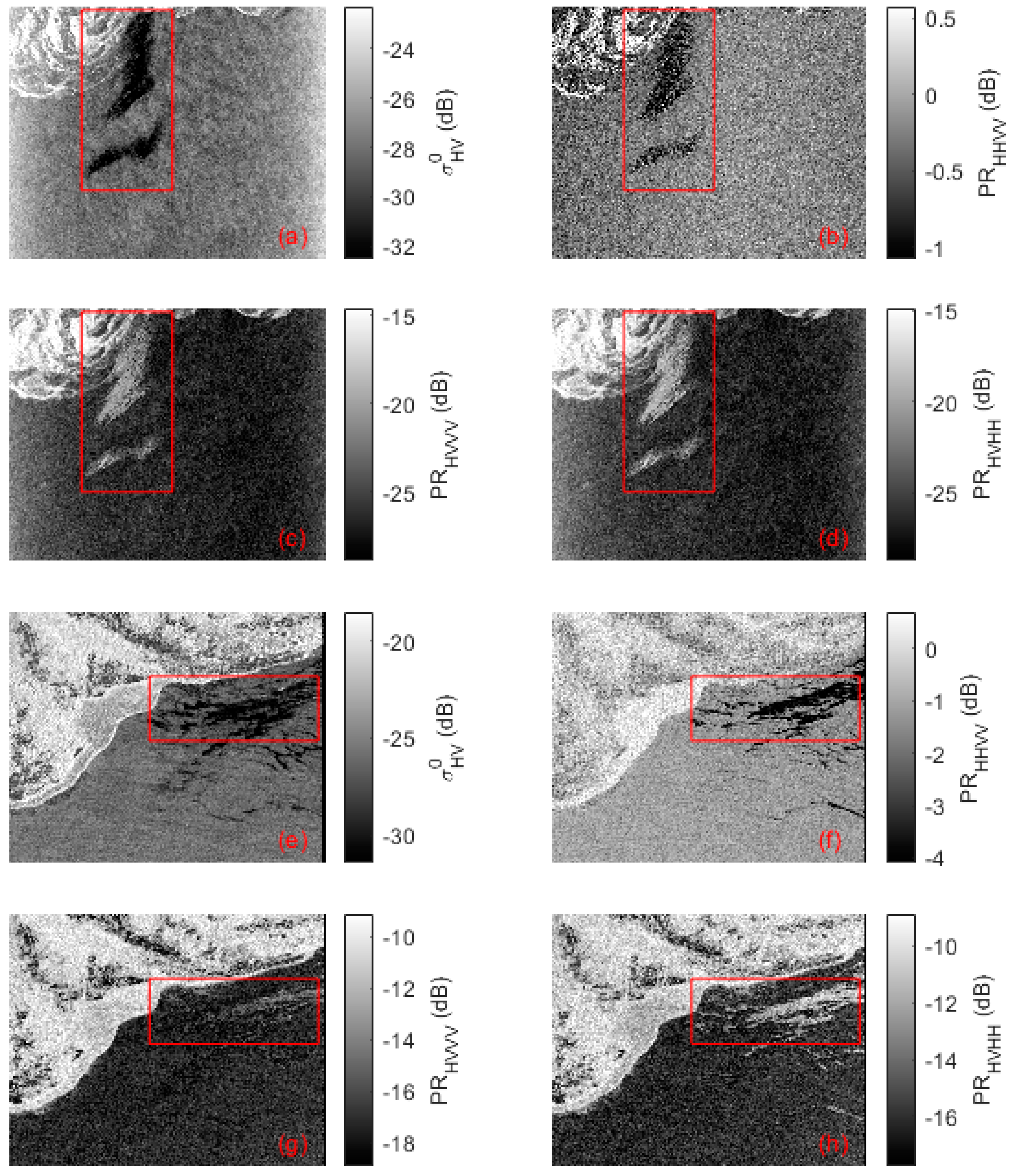
As shown in Figure 3a,e, low backscatter areas are sufficiently darker than the neighboring areas to be suitable for our methodology. The former are related to small sea surface roughness resulting from low wind speed, or alternatively oil spill areas. They have relatively low co-pol ratios (Figure 3b,f), but rather large cross-pol ratios (Figure 3c,d,g,h) which are close to those of sea ice. Therefore, they have a significantly negative effect on the classification accuracy and can be detected accurately. Most of the existing low backscatter detection methods are mainly based on local statistics for determining the darkness degree with respect to the neighboring areas [50,51,52]. In this work, a fixed global threshold is used to determine the low backscatter areas: if the HV-pol NRCS of a pixel is less than −30 dB, then the pixel is identified as belonging to a low backscatter area.
- (3)
- PR threshold estimation:
The classic and effective threshold selection method OTSU [53] is used for automatic PR image segmentation. It is based on the zeroth- and the first-order cumulative moments of gray-level histograms. The core idea of OTSU is to maximize the between-class variance:
where and are the zeroth- and the first-order cumulative moments of the histogram up to the Tth level, respectively. is the total mean level of the original image.
The optimal threshold is:
It should be noted that low backscatter areas are excluded in the PR threshold estimation.
- (4)
- Segmentation of PR images:
After determining the optimal segmentation threshold for each PR image, one can differentiate OW from sea ice based on PR. We first segment the PR image into two parts, A (PR ≤ T) and B (PR > T). Then, the HV-pol NRCS is used to help discriminate sea ice and OW. The discriminating criterion is: if , A is sea ice and B is OW, else A is OW and B is sea ice. The symbol denotes the averaging operator. Finally, low backscatter areas are recognized as OW.
- (5)
- Determination of the optimal sea ice detection result:
The methodology to automatically determine the optimal sea ice detection result from the three segmentation results obtained in step (4) is crucial in our method. We find that the HV-pol SAR images can exhibit sea ice/OW contrast clearly in most cases. Therefore, a naïve idea is that the optimal sea ice detection result should be similar to the HV-pol SAR image, visually. Consequently, the problem can be simplified to that of measuring the similarity between each sea ice detection result and the HV-pol SAR image. There exist numerous techniques for evaluating the likenesses between two images.
In this study, the widely used structural similarity index method (SSIM) is used to assess the similarity between two images. The structural similarity image quality concept is founded on the idea that the human visual system is well-suited for extracting structural details from a scene. As a result, a measure of structural similarity can effectively approximate perceived image quality. This approach captures the characteristics of object structure within a scene and represents distortion as a composite of three distinct elements: luminance, contrast and structure. Specifically, SSIM utilizes the mean intensity to approximate luminance, the standard deviation to estimate contrast and covariance to quantify structural similarity. SSIM is measured by combining three components, and is defined as [54]:
where , and are luminance, contrast and structure comparison functions, respectively. , and are used to adjust the relative importance of these three components. We set in this paper.
3. Results
3.1. Polarimetric Characteristics of Sea Ice and OW
3.1.1. Backscattering Characteristics of Sea Ice and OW
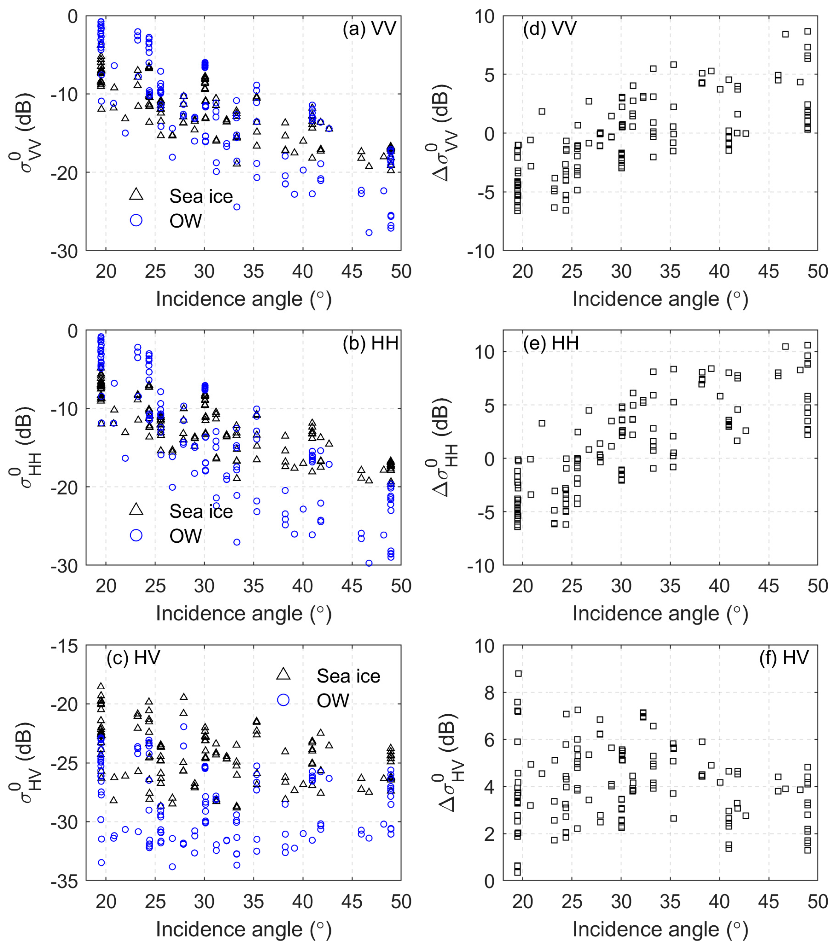
Figure 4a–c shows the NRCS of sea ice and OW in VV-, HH- and HV-pol, versus various radar incidence angles. It is clear that the NRCS of sea ice and OW in VV- and HH-pol have strong monotonically decreasing dependencies on incidence angles, while the incidence angle dependence of NRCS in HV-pol is relatively small. Figure 4d–f shows the NRCS difference () in VV-, HH- and HV-pol, versus incidence angles. Obviously, NRCS in VV- and HH-pol are not ideal indicators for discriminating OW from sea ice. As shown in Figure 4f, the HV-pol NRCS of sea ice is larger than that of OW for all incidence angle conditions. This indicates that HV-pol NRCS is a good discriminant factor for the sea ice detection task.
3.1.2. PR Characteristics of Sea Ice and OW
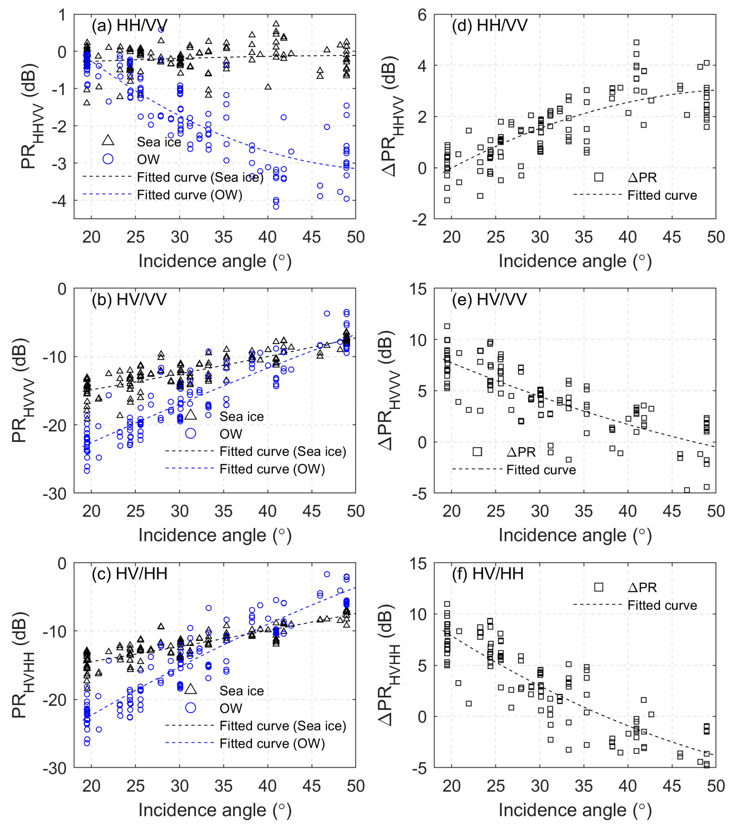
Figure 5a–c shows the PR of sea ice and OW versus incidence angles. The black and blue dashed lines represent the second-order fitting of the PR of sea ice and OW, respectively. For sea ice, incidence angles have a very small effect on the co-pol ratio () which is roughly distributed in the range of (−1, 1) dB. However, the co-pol ratio of OW decreases significantly with increasing incidence angles. For both sea ice and OW, a conspicuous monotonic increase can be found in the influence of incidence angles on two kinds of cross-pol ratio (, ), as shown in Figure 5b,c.
Figure 5d–f shows the PR difference between sea ice and OW (), versus incidence angles. The dashed lines denote the second-order fitting of the PR difference. Clearly, the co-pol ratio difference () increases with incidence angles, while both kinds of cross-pol ratio difference (, ) decrease with incidence angles and they have very similar variation trends. These results suggest that the co-pol ratio should be a good parameter for discriminating OW from sea ice under large incidence angle conditions, while the two kinds of cross-pol ratio have better differential capability in the case of small incidence angles. Therefore, we can develop a sea ice detection algorithm by realizing the full potential of the co-pol ratio and cross-pol ratios.
3.2. Accuracy Assesment
To validate our proposed method, manual visual interpretations have been carried out for all SAR images. In order to assess the effectiveness of the suggested approach for distinguishing between sea ice and water, we employ both statistical validation and case validation by comparing our classification results with manual visual interpretations. An overall accuracy metric is used to evaluate the classification accuracy. The overall accuracy is calculated as the proportion of correctly classified sea ice and open water pixels to the total number of pixels used for classification.
3.2.1. Statistical Validation
The classification accuracy of different classification methods based on a single PR parameter or PR combinations (ours) is evaluated by comparison with the visual interpretation results. The assessment results are shown in Table 2. The overall accuracy of the co-pol ratio and the two cross-pol ratios are 0.83, 0.79 and 0.77, respectively. Clearly, the classification accuracy of the co-pol ratio is higher than that of the two kinds of cross-pol ratio. Based on the combination of the co-pol ratio and the two kinds of cross-pol ratio, our proposed sea ice detection method achieves the best performance. The accuracy of our method is 96%, and improves 15.6–24.7% over single PR parameter-based methods.
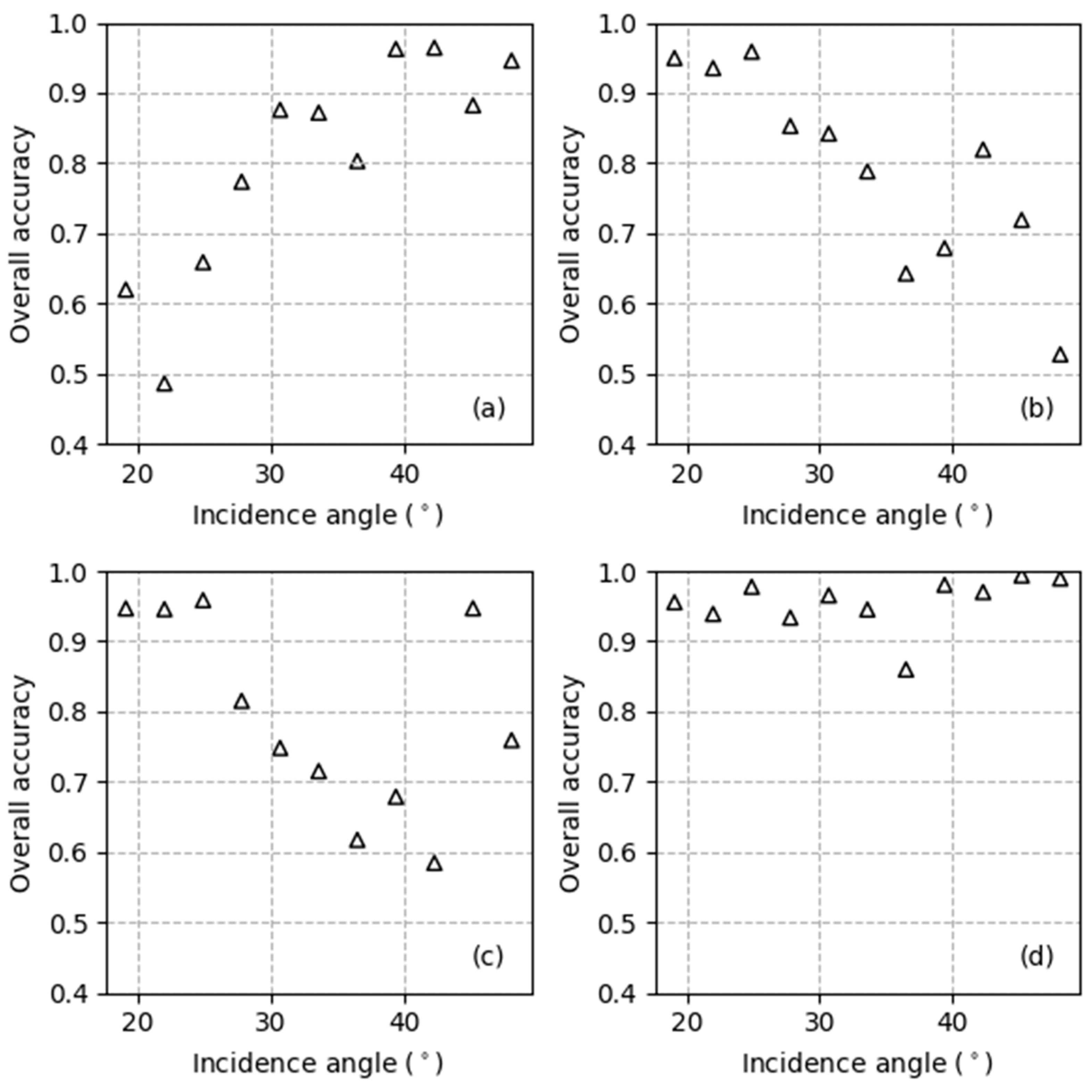
To study the incidence angle effects on the classification accuracy, we divide incidence angles into 11 equal intervals (2.9°) and perform accuracy evaluation over them. Figure 6 shows the overall accuracy of four PR methods at different incidence angles. As shown in Figure 6a–c, the co-pol ratio has high overall accuracy at large incidence angles, while the two cross-pol ratios perform better at small incidence angles. Based on the combination of the co-pol ratio and the two cross-pol ratios, our proposed method achieves high accuracy (>0.9) at almost all incidence angles.
3.2.2. Case Validation
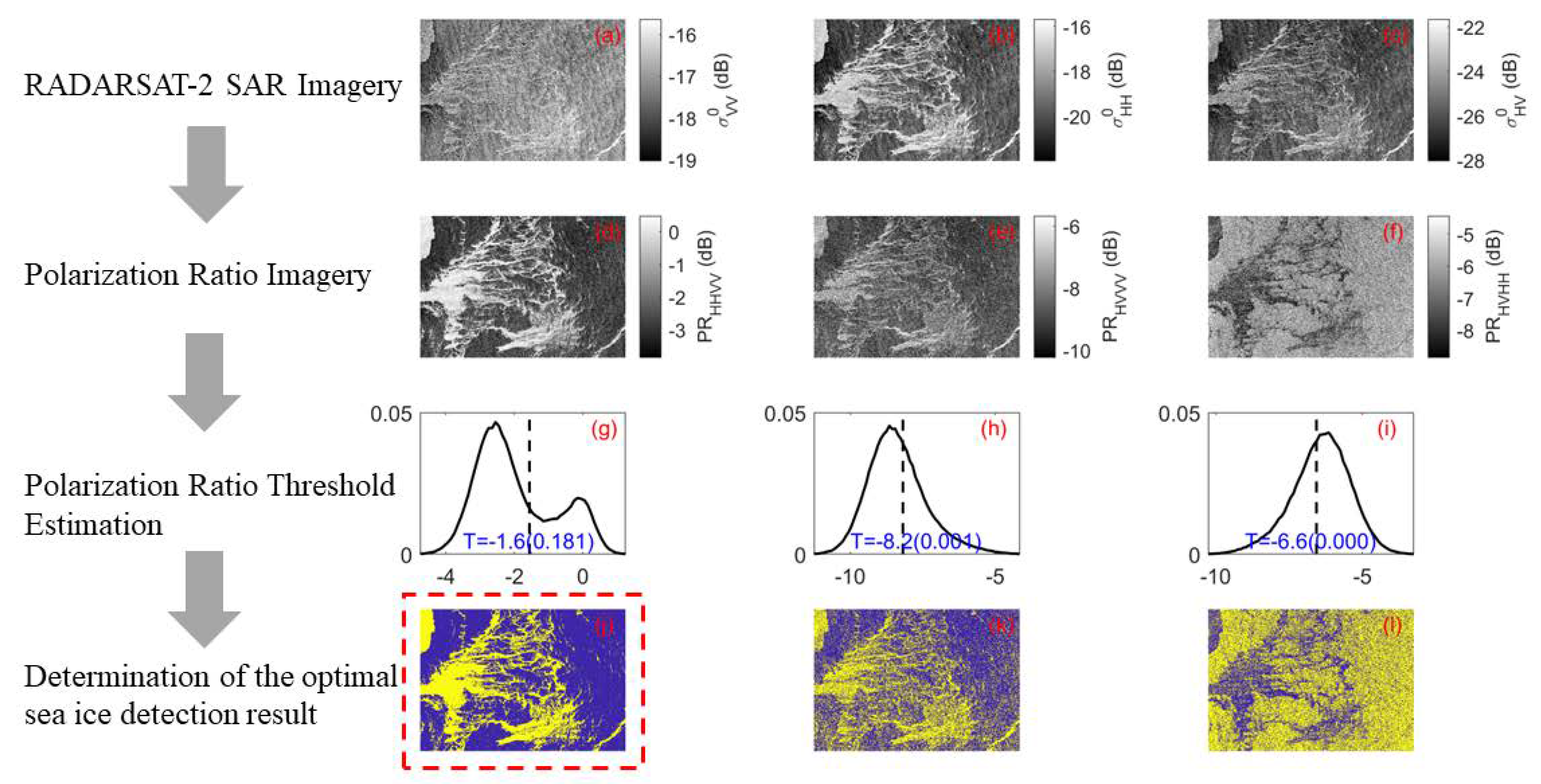
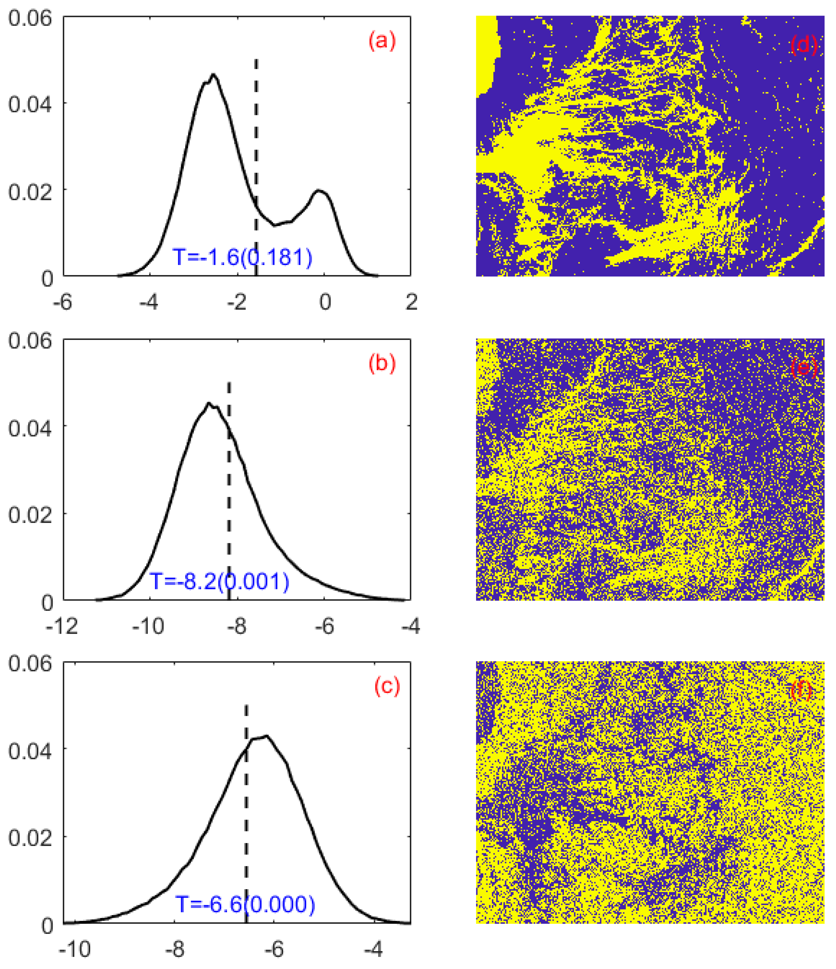
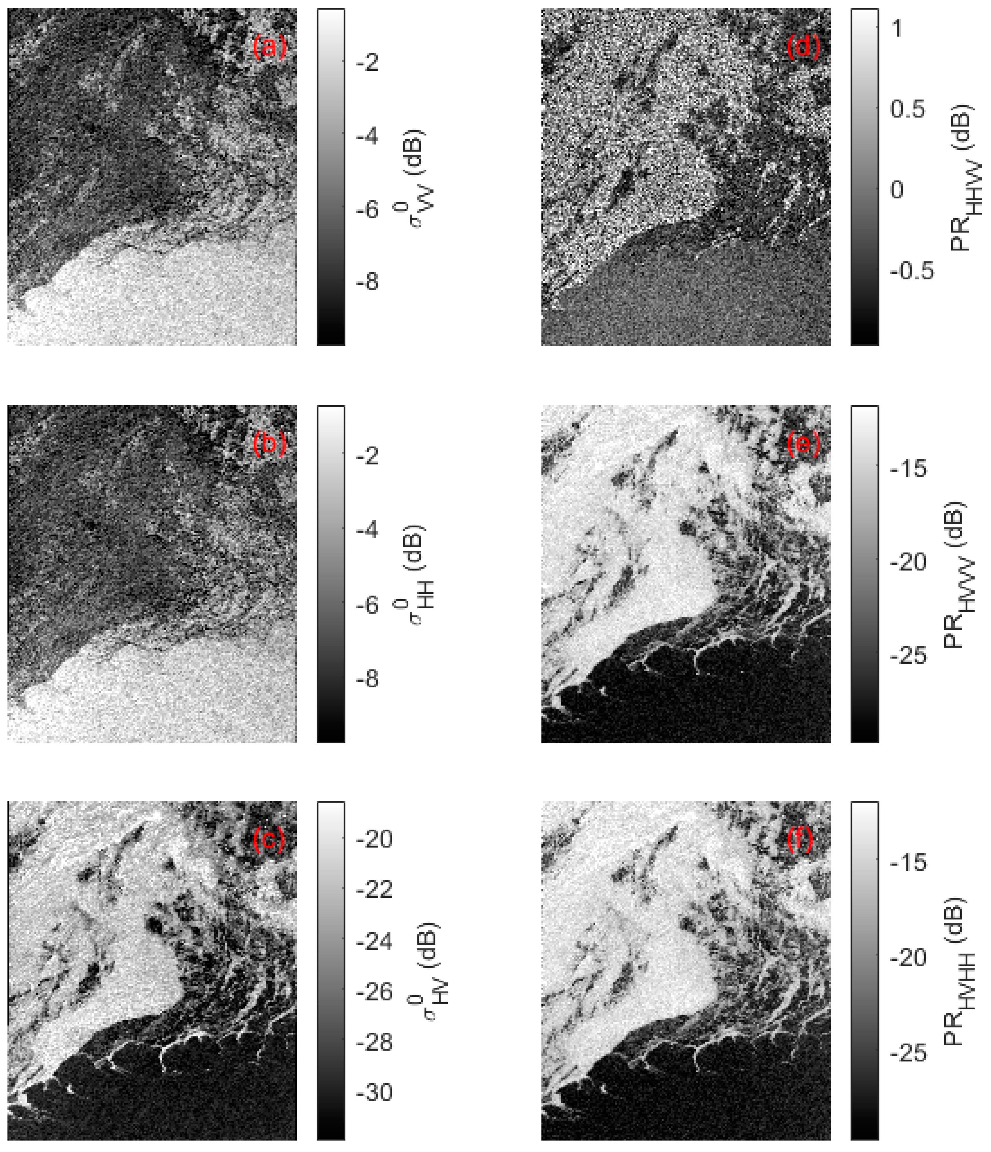
Figure 7a–c shows RADARSAT-2 VV-, HH- and HV-pol SAR images acquired on 11 July 2014, respectively. The incidence angles are in the range of 48.4° to 49.5°. Based on the C2PO wind speed retrieval model [55], we estimate the wind speed over the OW area from the HV-pol SAR image. The mean wind speed across the OW areas is 16.6 m/s. Under high wind conditions, the HH-pol SAR image shows a higher contrast between wind-roughened OW areas and sea ice than the VV-pol SAR image, due to its greater ability to suppress the sea cluster. For the HV-pol SAR image, radar returns from some ice-covered regions are very similar to those from OW areas. This is likely due to a decrease in volume scattering caused by a portion of the ice surface that is undergoing melting, or by a mixture of some ice floes and OW under strong wind conditions. Therefore, HH-pol is more suitable for sea ice detection than VV- and HV-pol in this case. Figure 7d–f shows the co-pol ratio and two kinds of cross-pol ratio images, respectively. Clearly, the co-pol ratio is more suitable for sea ice detection than the cross-pol ratios, due to a relatively larger difference between the co-pol ratio of sea ice and OW, at large incidence angles. To be specific, the average PR differences between sea ice and OW are 2.2 dB (HH/VV), 1.2 dB (HV/VV) and −1.0 dB (HV/HH), respectively. This high contrast characteristic of the co-pol ratio is very useful in sea ice detection, especially at high incidence angles (see Figure 5).
Figure 8a–c shows histograms of the co-pol ratio and the two cross-pol ratios corresponding to Figure 7d–f. The histogram of the co-pol ratio has two obvious peaks indicating sea ice and OW, which can be determined using the HV-pol SAR image, as mentioned in Section 2.3. In contrast, the histograms of the two cross-pol ratios have only one peak, making it hard to discriminate sea ice from OW. After applying the OTSU segmentation algorithm to the three PR images, we obtain three PR thresholds: −1.6 dB (HH/VV), −8.2 dB (HV/VV) and −6.6 dB (HV/HH). The corresponding segmentation results are shown in Figure 8d–f, respectively. Then, the SSIM values between the three detection results and HV-pol SAR image are estimated to determine the optimal sea ice detection results from the three PR-based segmentation results, automatically. They are 0.181, 0.001, 0.000 for the three detection results, respectively. Therefore, in this case, the best sea ice detection result is the co-pol ratio-based segmentation result. By comparing this sea ice detection result and the manual visual interpretation result, the overall accuracy is 0.97.
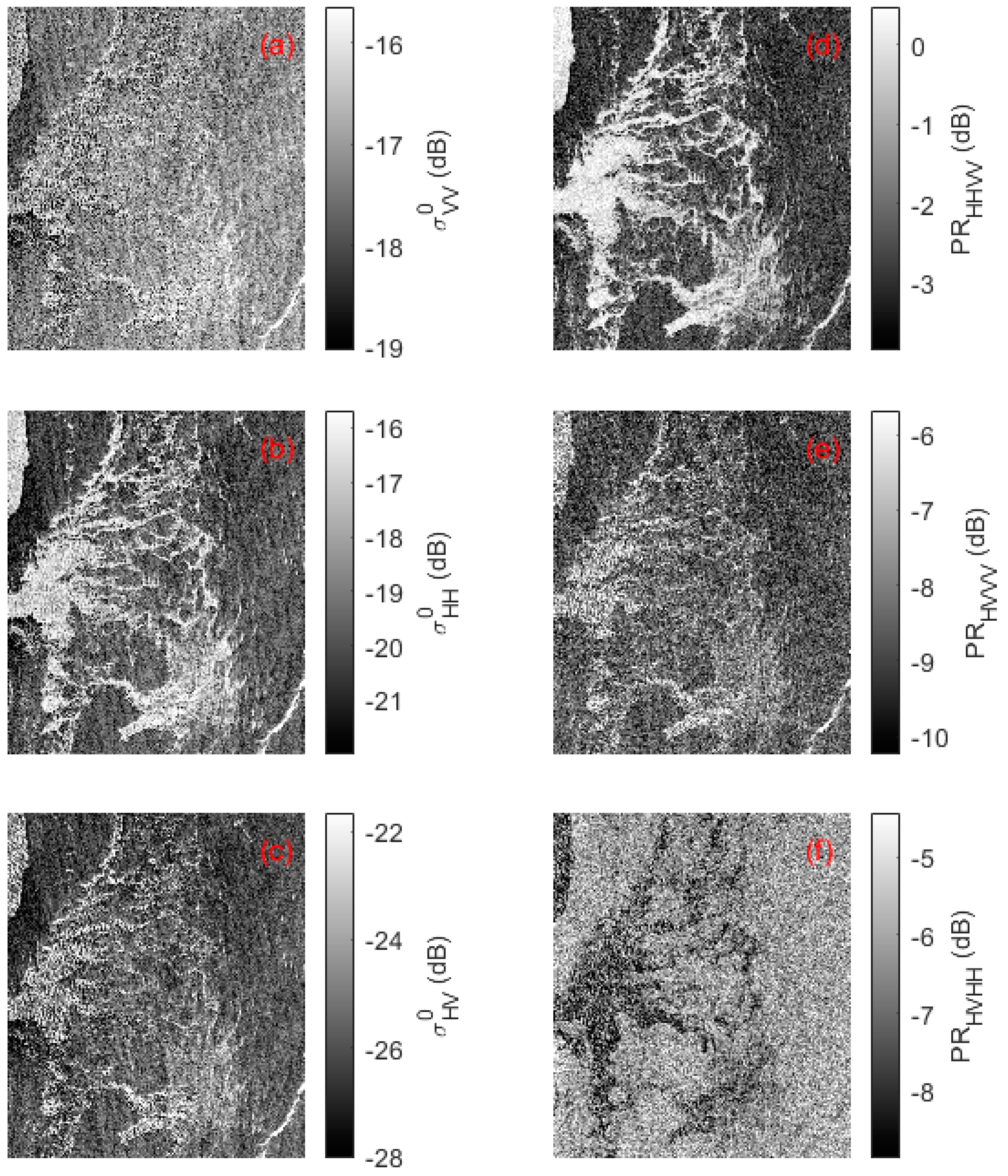
Figure 9a–c shows RADARSAT-2 VV-, HH- and HV-pol SAR images acquired on 1 December 2013. For this case, the incidence angles range from 18.6° to 20.4°. The wind speed in OW areas is estimated from the HV-pol SAR image, based on the C2PO model. The average wind speed is 14.5 m/s. As shown in Figure 9a,b, the VV- and HH-pol NRCS values of OW are even higher than those of the sea ice area due to high wind speeds. In the MIZ, the wind-roughened OW and sea ice have very similar radar intensities for both VV- and HH-pol. Consequently, it is quite difficult to use only VV- and HH-pol SAR images to detect sea ice and OW. By contrast, the HV-pol SAR image shows a higher contrast between sea ice and OW, because the HV-pol backscatter does not saturate at high wind speeds [55]. As such, the HV-pol is more appropriate for sea ice detection than VV- and HH-pol. Figure 9d–f shows the co-pol ratio and the two cross-pol ratio images, respectively. The OW and sea ice have very similar co-pol ratios, especially in the complicated MIZ, as shown in Figure 9d. Consequently, many sea ice details are lost in the MIZ in the co-pol ratio image. For the two cross-pol ratio images shown in Figure 9e,f, there is a higher sea ice-OW contrast. Moreover, the fine MIZ details can also be captured by these two cross-pol ratio images. Small ice floes are clearly seen in them. In particular, the average PR differences between sea ice and OW are calculated to be 0.8 dB for HH/VV, 6.1 dB for HV/VV and 5.3 dB for HV/HH. Therefore, the two cross-pol ratios are more suitable for identifying sea ice and OW than the co-pol ratio, especially at small incidence angles (see Figure 5).
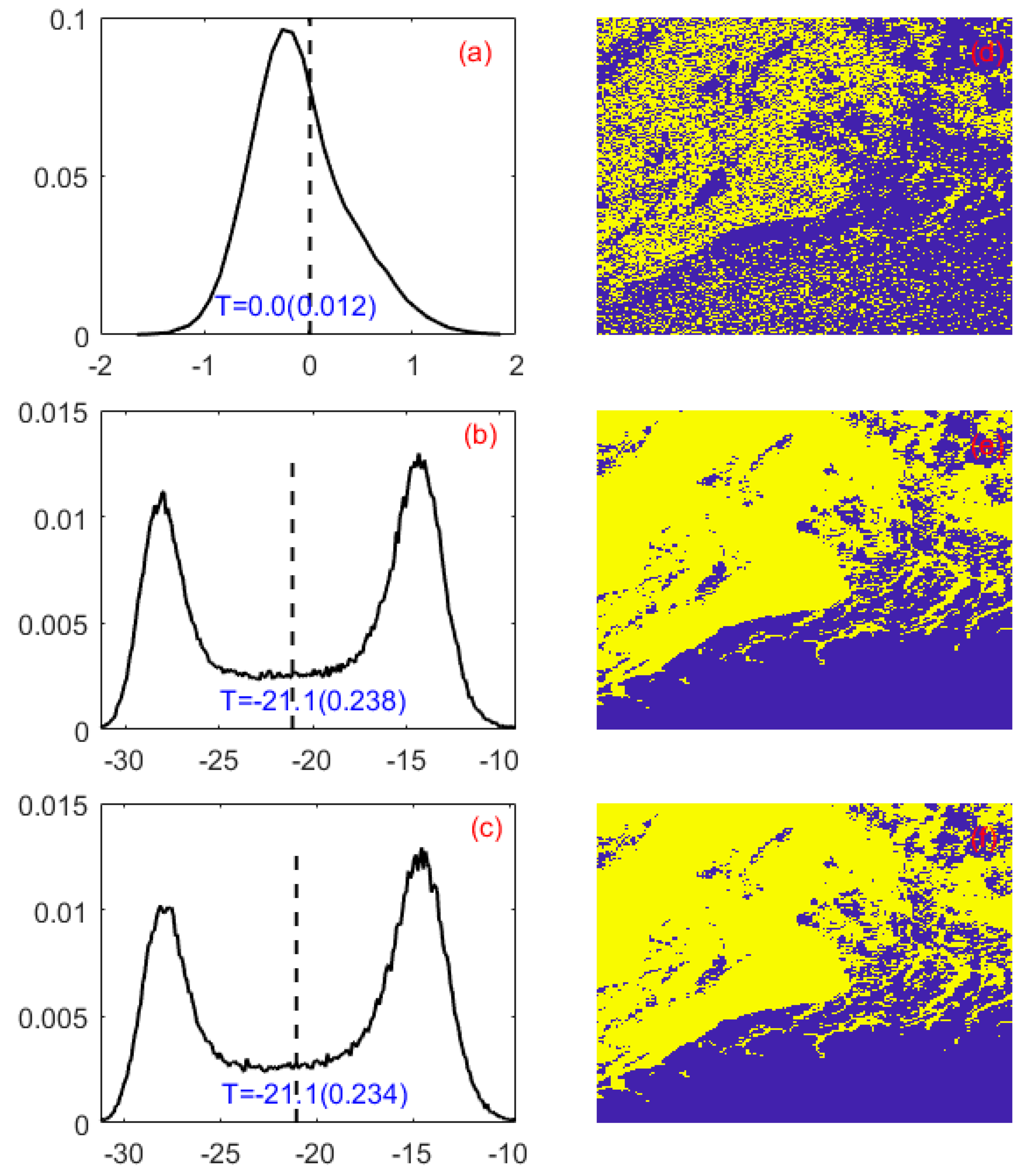
Figure 10a–c shows histograms of the co-pol ratio and the two cross-pol ratios corresponding to Figure 9d–f. The co-pol ratio exhibits a unimodal distribution, while the two cross-pol ratios have two distinct peaks which represent OW and sea ice. This indicates that, in this case, the two-cross pol ratios are more suitable for sea ice monitoring. Upon implementation of the OTSU segmentation algorithm on three PR images, three PR thresholds are derived: 0.0 dB for HH/VV, −21.1 dB for HV/VV and HV/HH. The resultant segmentation outcomes are depicted in Figure 10d–f, correspondingly. Next, the SSIM is calculated to assess the correspondence between the HV-pol SAR image and the sea ice detection results obtained from the three PR-based segmentation methods. The SSIM values for the three detection results are 0.012, 0.238 and 0.234, respectively. This means the sea ice detection results derived from the two cross-pol ratio images are better than those from the co-pol ratio images. The overall accuracy of the classification results is 0.95 for two cross-pol ratio-based detection results. In the MIZ, a small proportion of sea ice pixels are misclassified as OW.
4. Discussion
4.1. The Effectiveness of SSIM
As an important component of our method, how to determine the optimal sea ice detection result from single-PR-based results is critical. In this study, we use the SSIM index to determine the best classification result. This is necessary to evaluate the accuracy of this approach. Table 3 shows the accuracy evaluation matrix of the optimal result determination method, based on SSIM. The overall accuracy reaches 0.95, indicating the high reliability and accuracy of the method.
4.2. Effect of Incidence Angles on PR Threshold
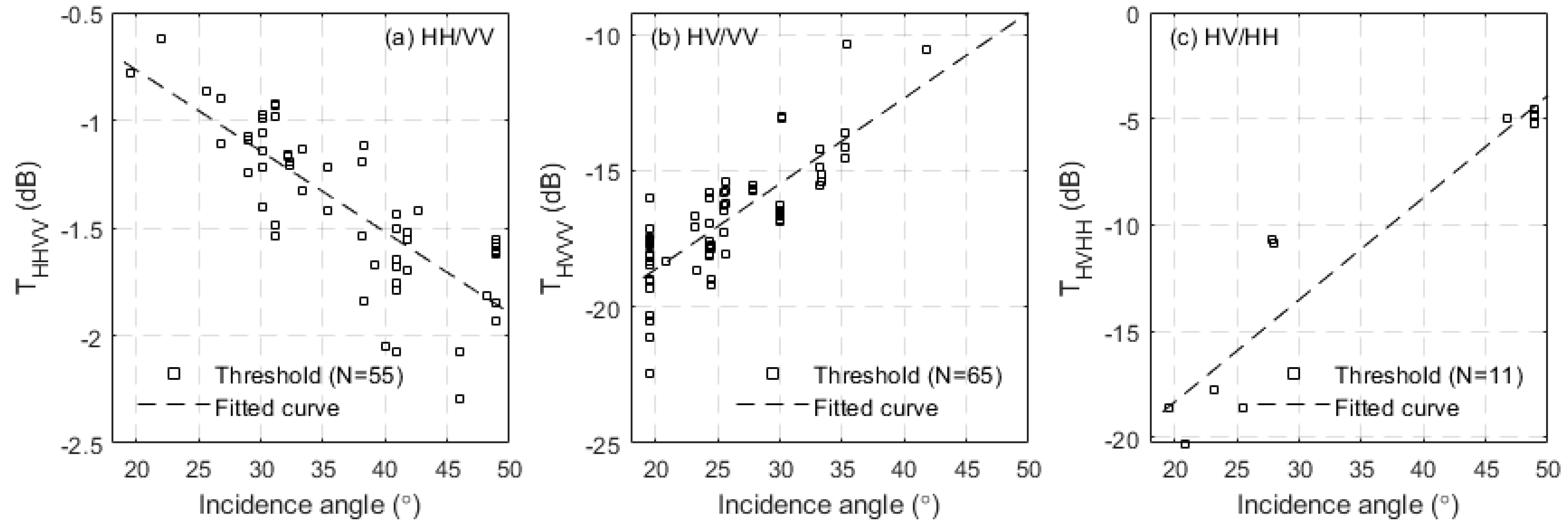
As the variation of incidence angles in RADARSAT-2 quad-polarization SAR images is quite small (~1.5°), the central incidence angle can be considered as the incidence angle of each SAR image. Figure 11 shows the variation of the optimal PR threshold with respect to radar incidence angles. Linear incidence angle dependence is observed for three kinds of PR threshold. The co-pol ratio threshold decreases with increasing incidence angles, while the two kinds of cross-pol ratio threshold have an opposite trend. This is reasonable and can be proven by Figure 5.
On the other hand, it can be seen from Figure 11a,b that the distribution of co-pol ratio thresholds and the cross-pol ratio (HV/VV) threshold are quite different with respect to incidence angles. The cross-pol ratio (HV/VV) threshold is mainly distributed at small incidence angles from 20° to 35°, while the co-pol ratio threshold tends to be distributed over a wider range of incidence angles from 25° to 50°. These results are consistent with the distribution of the PR difference between sea ice and OW, as shown in Figure 5d,e.
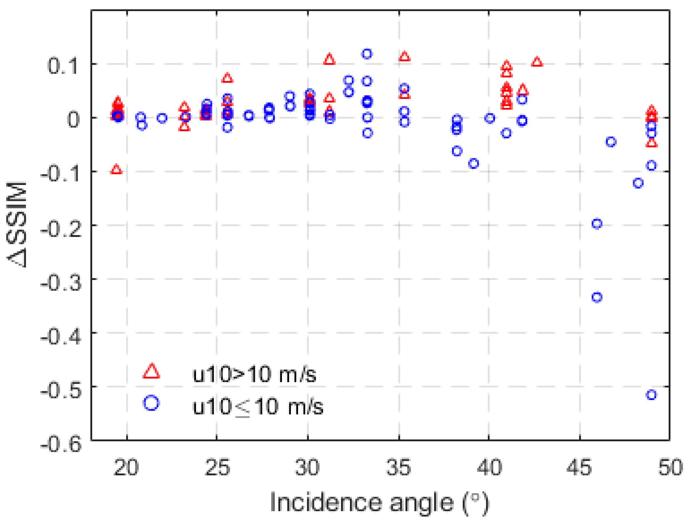
As shown in Figure 11c, the number of cross-pol ratio (HV/HH) thresholds is far less than that of the cross-pol ratio (HV/VV) thresholds. Does this mean the performance of the cross-pol ratio (HV/VV) is significantly higher than that of the cross-pol ratio (HV/HH)? In fact, there is no significant accuracy difference between them, as shown in Table 2. To explain this result, Figure 12 shows the SSIM difference () between the two kinds of cross-pol ratio. Obviously, there is no significant SSIM difference between them at small incidence angles (<30°). This can demonstrate that the cross-pol ratio (HV/HH) is also able to achieve good performance at small incidence angles. For large incidence angles, the cross-pol ratio (HV/VV) tends to perform better at high wind speeds, while the cross-pol ratio (HV/HH) has a better performance at low wind speeds. We will further explain the effect of incidence angles and wind conditions on PR in the discussion section.
4.3. The Wind Effects on PR
The co-pol and cross-pol NRCS of OW are dependent on incidence angles, wind speeds and wind directions. Many electromagnetic scattering models have been developed to estimate radar backscatters induced by OW, considering both incidence angles and wind effects. For example, the composite surface Bragg (CB) model [56] and the small slope approximation (SSA) model [57] are widely used in the simulation of electromagnetic interactions with OW. However, a recent study has demonstrated that these models give underestimates, especially for HH- and HV-pol NRCS due to neglect of the effect of breaking waves. The contribution of breaking waves can achieve up to 60–70% of the total NRCS for HH- and HV-pol, for all incidence angles at C-band [48].
As well as theoretical electromagnetic scattering models, many empirical geophysical model functions (GMFs) have been proposed to model co-pol and cross-pol NRCS of OW, with the inputs of incidence angles, wind speeds and wind directions. They are developed based on SAR-measured NRCS and collocated winds from in situ buoys, scatterometers and radiometers. As a result, the NRCSs derived from GMFs have better agreement with SAR observations than those from electromagnetic scattering models. Therefore, we adopt empirical GMFs to simulate the co-pol and cross-pol NRCSs of OW in this work. We employ the CMOD5.N [58], CMODH [59] and C3PO [60] GMFs to estimate VV-, HH- and HV-pol NRCS of OW, respectively. The formulations of these GMFs are given in Appendix A. Then, the co-pol ratio and cross-pol ratio of OW can be calculated based on simulated NRCS results. The PR of sea ice is estimated by fitting observational results.
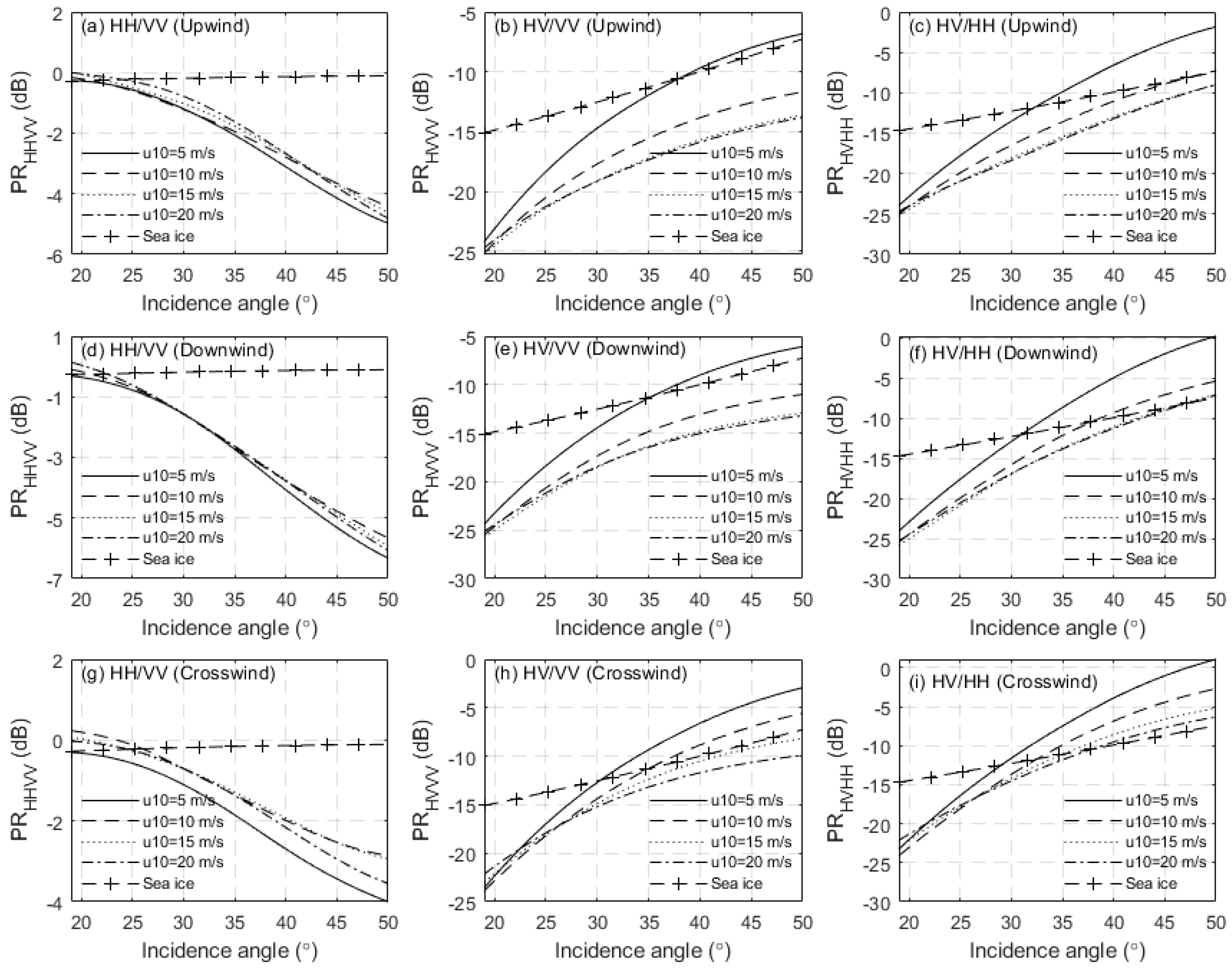
As shown in Figure 13a,d,g, the wind effects can be neglected for the co-pol ratio. The PR difference between sea ice and OW is small at small incidence angles and increases with incidence angles. In particular, this implies that the ability of the co-pol ratio to distinguish sea ice from OW increases with incidence angles.
For the cross-pol ratio, the HV/VV and HV/HH results shown in Figure 13b,c,e,f,h,i indicate that wind conditions have significant effects on the cross-pol ratio of OW. The cross-pol ratio of OW increases with wind speeds. At small incidence angles, wind effects can be ignored. A relatively large PR difference is observed between sea ice and OW at small incidence angles (upwind and downwind: <35°, crosswind: <30°). This suggests that the cross-pol ratio is better than the co-pol ratio for sea ice detection at small incidence angles. When incidence angles exceed 35°, wind speeds and wind directions will significantly influence the ability of the cross-pol ratio to detect sea ice. For example, Figure 13b,e suggests that the cross-pol ratio HV/VV has a better capability to distinguish OW at high wind speeds, for upwind and downwind conditions. Figure 13c,f,i shows that the cross-pol ratio HV/HH has a better performance at low wind speeds.
4.4. Performance Comparison to Other Algorithms
Many PR-based sea ice detection methods have been developed for sea ice and OW discrimination, such as decision tree [23], k-means [22,24] and the X-Bragg backscatter model [47]. Since their classification performances were evaluated on small datasets, it is necessary to reassess their accuracy using our larger datasets. Table 4 shows the performance evaluation results for these different sea ice detection algorithms. It can be found that the performance of these methods based on a single PR parameter is significantly poorer than our proposed algorithm. Due to the incidence angle effects on PR, as shown in Figure 5, a single PR parameter cannot work well for all incidence angle ranges. However, the combination of multiple PR parameters can solve this problem, almost perfectly, by utilizing and combining their own individual advantages.
4.5. Future Work
The RADARSAT-2 quad-polarization SAR data have the advantage of very high spatial resolution. The main limitation is its long revisit time, up to 24 days. Moreover, the swath width of RADARSAT-2 quad-polarization SAR data is limited to a relatively small range of 25–50 km because of the doubled pulse repetition frequency and the alternate transmission of orthogonal linear polarization pulses, such as horizontal (H) and vertical (V) polarizations. These disadvantages limit its application in large-scale sea ice detection. More recently, the RADARSAT Constellation Mission has been launched successfully on 12 June 2019. The RCM represents an advancement of the RADARSAT program, aiming to maintain the continuity of data from previous RADARSAT missions. RCM consists of three identical C-Band SAR satellites. The arrangement of three satellites allows for frequent coverage of Canada’s extensive land and maritime regions, including the Arctic, with up to four passes per day. It can also provide daily monitoring of 90% of the Earth’s surface. The RCM quad-polarization SAR range has a wide swath width, up to 250 km. Therefore, the RCM quad-polarization data have rather good spatial and temporal resolution, as well as a large swath width. We will further investigate the effectiveness of our method using RCM quad-polarization data. In addition, the RCM compact polarimetry data can also be used to develop a sea ice detection algorithm based on the basic idea of this work. We will further investigate this topic in our forthcoming research.
5. Conclusions
In this paper, we present an analysis of the polarimetric characteristics, such as backscattering characteristics and PR characteristics, of sea ice and OW. The statistical results indicate that the HV-pol NRCS is a useful parameter in sea ice detection (Figure 4f). The co-pol ratio difference between sea ice and OW increases with incidence angles, while the two kinds of cross-pol ratio difference decrease with incidence angles. The results suggest that the co-pol ratio is suitable for sea ice detection at large incidence angles while the two kinds of cross-pol ratio are more applicable to sea ice detection at small incidence angles.
Based on the above analysis results, an automatic sea ice detection method is proposed based on co-pol and cross-pol ratios, as well as an auxiliary parameter: HV-pol NRCS. Compared with visual interpretation results, our method shows promising results with a high accuracy of 96%. As expected, there is a linear dependence between the PR threshold and incidence angles. Experimental results show that the co-pol ratio has a better performance at a wide range of incidence angles from 25° to 50°, while the cross-pol ratio is more effective in sea ice detection at small incidence angles, from 20° to 35°. Based on the GMFs of OW, the numerical results further validate our findings. Compared with previous works, the accuracy of our method is much higher than that of single PR parameter-based methods.
The RADARSAT-2 quad-polarization SAR data have the benefit of extremely high spatial resolution. However, RADARSAT-2 quad-pol data are limited due to the long revisit time and small swath width, making it hard to perform large-scale sea ice detection. The new generation RCM data shortens the revisit time to about one day, and the maximum swath width for the quad-polarization mode can be 250 km. In the future, we will validate the effectiveness of our method using RCM quad-polarization data. Furthermore, we will also develop a sea ice detection algorithm based on RCM compact-polarization data.
Author Contributions
Conceptualization, L.Z. and T.X.; methodology, L.Z.; software, L.Z.; validation, L.Z., T.X. and W.P.; formal analysis, W.P.; investigation, L.Z.; resources, W.P.; data curation, T.X.; writing—original draft preparation, L.Z.; writing—review and editing, W.P. and J.Y.; visualization, L.Z.; supervision, T.X.; project administration, T.X.; funding acquisition, T.X. All authors have read and agreed to the published version of the manuscript.
Funding
This research was funded by the National Key R&D Program of China under grant number 2021YFC2803302 and 2022YFC3104900, and the National Natural Science Foundation of China project under grant number 42176180.
Data Availability Statement
The RADARSAT-2 SAR images are provided by Canadian Space Agency, which can be acquired from Earth Observation Data Management System (https://www.eodms-sgdot.nrcan-rncan.gc.ca, accessed on 28 January 2024), and the ERA5 data are from the European Centre for Medium-Range Weather Forecasts (https://www.ecmwf.int/, accessed on 28 January 2024).
Acknowledgments
We thank the Canadian Space Agency for providing access to RADARSAT-2 SAR imagery and the European Centre for Medium-Range Weather Forecasts for ERA5 reanalysis data.
Conflicts of Interest
The authors declare no conflicts of interest.
Appendix A
The CMOD5.N and CMODH GMFs are functions of incidence angles, wind speeds and wind directions, which are given as [58,59]:
where for CMOD5.N and for CMODH. , , are functions of incidence angles and wind speeds . is defined as:
where:
where:
The functions , , , , depend on incidence angles only.
where .
is defined as:
is defined as:
is given by:
where:
, , are functions of incidence angles.
The coefficients are given in Table A1.

Table A1.
Coefficients of CMOD5.N and CMODH.
| Function | Coefficients | CMOD5.N | CMODH |
|---|---|---|---|
| −0.6878 | −0.7272 | ||
| −0.7957 | −1.1901 | ||
| 0.3380 | 0.3396 | ||
| −0.1728 | 0.0867 | ||
| 0.0000 | 0.0030 | ||
| 0.0040 | 0.0117 | ||
| 0.1103 | 0.1291 | ||
| 0.0159 | 0.0835 | ||
| 6.7329 | 4.0925 | ||
| 2.7713 | 1.2111 | ||
| −2.2885 | −1.1197 | ||
| 0.4971 | 0.5790 | ||
| −0.7250 | −0.6045 | ||
| 0.0450 | 0.1183 | ||
| 0.0066 | 0.0089 | ||
| 0.3222 | 0.2196 | ||
| 0.0120 | 0.0175 | ||
| 22.700 | 24.442 | ||
| 2.0813 | 1.9834 | ||
| 3.0000 | 6.7814 | ||
| 8.3659 | 7.9479 | ||
| −3.3428 | −4.6964 | ||
| 1.3236 | −0.4370 | ||
| 6.2437 | 5.4712 | ||
| 2.3893 | 0.6394 | ||
| 0.3249 | 0.6733 | ||
| 4.1590 | 3.4332 | ||
| 1.6930 | 0.3670 |
The C3PO model is defined as [60]:
References
- DeRepentigny, P.; Jahn, A.; Holland, M.M.; Smith, A. Arctic sea ice in two configurations of the CESM2 during the 20th and 21st centuries. J. Geophys. Res. Oceans 2020, 125, e2020JC016133. [Google Scholar] [CrossRef]
- Lannuzel, D.; Tedesco, L.; Van Leeuwe, M.; Campbell, K.; Flores, H.; Delille, B.; Miller, L.; Stefels, J.; Assmy, P.; Bowman, J. The future of Arctic sea-ice biogeochemistry and ice-associated ecosystems. Nat. Clim. Chang. 2020, 10, 983–992. [Google Scholar] [CrossRef]
- Notz, D.; Community, S. Arctic sea ice in CMIP6. Geophys. Res. Lett. 2020, 47, e2019GL086749. [Google Scholar] [CrossRef]
- Cai, Q.; Wang, J.; Beletsky, D.; Overland, J.; Ikeda, M.; Wan, L. Accelerated decline of summer Arctic sea ice during 1850–2017 and the amplified Arctic warming during the recent decades. Environ. Res. Lett. 2021, 16, 034015. [Google Scholar] [CrossRef]
- Comiso, J.C.; Parkinson, C.L.; Gersten, R.; Stock, L. Accelerated decline in the Arctic sea ice cover. Geophys. Res. Lett. 2008, 35, L01703. [Google Scholar] [CrossRef]
- Liu, Z.; Risi, C.; Codron, F.; He, X.; Poulsen, C.J.; Wei, Z.; Chen, D.; Li, S.; Bowen, G.J. Acceleration of western Arctic sea ice loss linked to the Pacific North American pattern. Nat. Commun. 2021, 12, 1519. [Google Scholar] [CrossRef] [PubMed]
- Tivy, A.; Howell, S.E.; Alt, B.; McCourt, S.; Chagnon, R.; Crocker, G.; Carrieres, T.; Yackel, J.J. Trends and variability in summer sea ice cover in the Canadian Arctic based on the Canadian Ice Service Digital Archive, 1960–2008 and 1968–2008. J. Geophys. Res. Ocean. 2011, 116, C03007. [Google Scholar] [CrossRef]
- Wang, Z.; Li, Z.; Zeng, J.; Liang, S.; Zhang, P.; Tang, F.; Chen, S.; Ma, X. Spatial and temporal variations of Arctic sea ice from 2002 to 2017. Earth Space Sci. 2020, 7, e2020EA001278. [Google Scholar] [CrossRef]
- Kwok, R.; Spreen, G.; Pang, S. Arctic sea ice circulation and drift speed: Decadal trends and ocean currents. J. Geophys. Res. Ocean 2013, 118, 2408–2425. [Google Scholar] [CrossRef]
- Chylek, P.; Folland, C.; Klett, J.D.; Wang, M.; Hengartner, N.; Lesins, G.; Dubey, M.K. Annual mean arctic amplification 1970–2020: Observed and simulated by CMIP6 climate models. Geophys. Res. Lett. 2022, 49, e2022GL099371. [Google Scholar] [CrossRef]
- Walsh, J.E.; Ballinger, T.J.; Euskirchen, E.S.; Hanna, E.; Mård, J.; Overland, J.E.; Tangen, H.; Vihma, T. Extreme weather and climate events in northern areas: A review. Earth-Sci. Rev. 2020, 209, 103324. [Google Scholar] [CrossRef]
- Christensen, T.; Lund, M.; Skov, K.; Abermann, J.; López-Blanco, E.; Scheller, J.; Scheel, M.; Jackowicz-Korczynski, M.; Langley, K.; Murphy, M. Multiple ecosystem effects of extreme weather events in the Arctic. Ecosystems 2021, 24, 122–136. [Google Scholar] [CrossRef]
- Cavalieri, D.J.; Gloersen, P.; Campbell, W.J. Determination of sea ice parameters with the Nimbus 7 SMMR. J. Geophys. Res. Atmos. 1984, 89, 5355–5369. [Google Scholar] [CrossRef]
- Markus, T.; Cavalieri, D.J. An enhancement of the NASA Team sea ice algorithm. IEEE Trans. Geosci. Remote Sens. 2000, 38, 1387–1398. [Google Scholar] [CrossRef]
- Comiso, J.; Sullivan, C. Satellite microwave and in situ observations of the Weddell Sea ice cover and its marginal ice zone. J. Geophys. Res. Ocean. 1986, 91, 9663–9681. [Google Scholar] [CrossRef]
- Andersen, S.; Tonboe, R.; Kern, S.; Schyberg, H. Improved retrieval of sea ice total concentration from spaceborne passive microwave observations using numerical weather prediction model fields: An intercomparison of nine algorithms. Remote Sens. Environ. 2006, 104, 374–392. [Google Scholar] [CrossRef]
- Svendsen, E.; Matzler, C.; Grenfell, T.C. A model for retrieving total sea ice concentration from a spaceborne dual-polarized passive microwave instrument operating near 90 GHz. Int. J. Remote Sens. 1987, 8, 1479–1487. [Google Scholar] [CrossRef]
- Spreen, G.; Kaleschke, L.; Heygster, G. Sea ice remote sensing using AMSR-E 89-GHz channels. J. Geophys. Res. Ocean. 2008, 113, C02S03. [Google Scholar] [CrossRef]
- Shokr, M.; Lambe, A.; Agnew, T. A new algorithm (ECICE) to estimate ice concentration from remote sensing observations: An application to 85-GHz passive microwave data. IEEE Trans. Geosci. Remote Sens. 2008, 46, 4104–4121. [Google Scholar] [CrossRef]
- Shokr, M.; Dabboor, M. Polarimetric SAR Applications of Sea Ice: A Review. IEEE J. Sel. Top. Appl. Earth Obs. Remote Sens. 2023, 16, 6627–6641. [Google Scholar] [CrossRef]
- Lyu, H.; Huang, W.; Mahdianpari, M. A meta-analysis of sea ice monitoring using spaceborne polarimetric SAR: Advances in the last decade. IEEE J. Sel. Top. Appl. Earth Obs. Remote Sens. 2022, 15, 6158–6179. [Google Scholar] [CrossRef]
- Gill, J.P.; Yackel, J.J. Evaluation of C-band SAR polarimetric parameters for discrimination of first-year sea ice types. Can. J. Remote Sens. 2012, 38, 306–323. [Google Scholar] [CrossRef]
- Geldsetzer, T.; Yackel, J. Sea ice type and open water discrimination using dual co-polarized C-band SAR. Can. J. Remote Sens. 2009, 35, 73–84. [Google Scholar] [CrossRef]
- Gill, J.P.; Yackel, J.J.; Geldsetzer, T. Analysis of consistency in first-year sea ice classification potential of C-band SAR polarimetric parameters. Can. J. Remote Sens. 2013, 39, 101–117. [Google Scholar] [CrossRef]
- Dabboor, M.; Montpetit, B.; Howell, S. Assessment of the high resolution SAR mode of the RADARSAT constellation mission for first year ice and multiyear ice characterization. Remote Sens. 2018, 10, 594. [Google Scholar] [CrossRef]
- Liu, H.; Guo, H.; Zhang, L. SVM-based sea ice classification using textural features and concentration from RADARSAT-2 dual-pol ScanSAR data. IEEE J. Sel. Top. Appl. Earth Obs. Remote Sens. 2015, 8, 1601–1613. [Google Scholar] [CrossRef]
- Zakhvatkina, N.; Korosov, A.; Muckenhuber, S.; Sandven, S.; Babiker, M. Operational algorithm for ice–water classification on dual-polarized RADARSAT-2 images. Cryosphere 2017, 11, 33–46. [Google Scholar] [CrossRef]
- Zhang, L.; Liu, H.; Gu, X.; Guo, H.; Chen, J.; Liu, G. Sea ice classification using TerraSAR-X ScanSAR data with removal of scalloping and interscan banding. IEEE J. Sel. Top. Appl. Earth Obs. Remote Sens. 2019, 12, 589–598. [Google Scholar] [CrossRef]
- Park, J.-W.; Korosov, A.A.; Babiker, M.; Won, J.-S.; Hansen, M.W.; Kim, H.-C. Classification of sea ice types in Sentinel-1 synthetic aperture radar images. Cryosphere 2019, 14, 2629–2645. [Google Scholar] [CrossRef]
- Lu, Y.; Zhang, B.; Perrie, W. Arctic Sea Ice and Open Water Classification from Spaceborne Fully Polarimetric Synthetic Aperture Radar. IEEE Trans. Geosci. Remote Sens. 2023, 61, 4203713. [Google Scholar] [CrossRef]
- Leigh, S.; Wang, Z.; Clausi, D.A. Automated ice–water classification using dual polarization SAR satellite imagery. IEEE Trans. Geosci. Remote Sens. 2014, 52, 5529–5539. [Google Scholar] [CrossRef]
- Zhu, T.; Li, F.; Heygster, G.; Zhang, S. Antarctic sea-ice classification based on conditional random fields from RADARSAT-2 dual-polarization satellite images. IEEE J. Sel. Top. Appl. Earth Obs. Remote Sens. 2016, 9, 2451–2467. [Google Scholar] [CrossRef]
- Li, X.-M.; Sun, Y.; Zhang, Q. Extraction of sea ice cover by Sentinel-1 SAR based on support vector machine with unsupervised generation of training data. IEEE Trans. Geosci. Remote Sens. 2020, 59, 3040–3053. [Google Scholar] [CrossRef]
- Mahmud, M.S.; Nandan, V.; Singha, S.; Howell, S.E.; Geldsetzer, T.; Yackel, J.; Montpetit, B. C-and L-band SAR signatures of Arctic sea ice during freeze-up. Remote Sens. Environ. 2022, 279, 113129. [Google Scholar] [CrossRef]
- Deng, H.; Clausi, D.A. Unsupervised segmentation of synthetic aperture radar sea ice imagery using a novel Markov random field model. IEEE Trans. Geosci. Remote Sens. 2005, 43, 528–538. [Google Scholar] [CrossRef]
- Boulze, H.; Korosov, A.; Brajard, J. Classification of sea ice types in Sentinel-1 SAR data using convolutional neural networks. Remote Sens. 2020, 12, 2165. [Google Scholar] [CrossRef]
- Khaleghian, S.; Ullah, H.; Kræmer, T.; Hughes, N.; Eltoft, T.; Marinoni, A. Sea ice classification of SAR imagery based on convolution neural networks. Remote Sens. 2021, 13, 1734. [Google Scholar] [CrossRef]
- Lyu, H.; Huang, W.; Mahdianpari, M. Eastern Arctic Sea Ice Sensing: First Results from the RADARSAT Constellation Mission Data. Remote Sens. 2022, 14, 1165. [Google Scholar] [CrossRef]
- Zhang, J.; Zhang, W.; Hu, Y.; Chu, Q.; Liu, L. An improved sea ice classification algorithm with Gaofen-3 dual-polarization SAR data based on deep convolutional neural networks. Remote Sens. 2022, 14, 906. [Google Scholar] [CrossRef]
- de Gelis, I.; Colin, A.; Longepe, N. Prediction of categorized sea ice concentration from Sentinel-1 SAR images based on a fully convolutional network. IEEE J. Sel. Top. Appl. Earth Obs. Remote Sens. 2021, 14, 5831–5841. [Google Scholar] [CrossRef]
- Radhakrishnan, K.; Scott, K.A.; Clausi, D.A. Sea Ice Concentration Estimation: Using Passive Microwave and SAR Data With a U-Net and Curriculum Learning. IEEE J. Sel. Top. Appl. Earth Obs. Remote Sens. 2021, 14, 5339–5351. [Google Scholar] [CrossRef]
- Ren, Y.; Li, X.; Yang, X.; Xu, H. Development of a dual-attention U-Net model for sea ice and open water classification on SAR images. IEEE Geosci. Remote Sens. Lett. 2022, 19, 4010205. [Google Scholar] [CrossRef]
- Zhao, L.; Xie, T.; Perrie, W.; Yang, J. Deep Learning-Based Sea Ice Classification with Sentinel-1 and AMSR-2 Data. IEEE J. Sel. Top. Appl. Earth Obs. Remote Sens. 2023, 16, 5514–5525. [Google Scholar] [CrossRef]
- Wan, H.; Luo, X.; Wu, Z.; Qin, X.; Chen, X.; Li, B.; Shang, J.; Zhao, D. Multi-Featured Sea Ice Classification with SAR Image Based on Convolutional Neural Network. Remote Sens. 2023, 15, 4014. [Google Scholar] [CrossRef]
- Nghiem, S.; Bertoia, C. Study of multi-polarization C-band backscatter signatures for Arctic sea ice mapping with future satellite SAR. Can. J. Remote Sens. 2001, 27, 387–402. [Google Scholar] [CrossRef]
- Dierking, W. Mapping of different sea ice regimes using images from Sentinel-1 and ALOS synthetic aperture radar. IEEE Trans. Geosci. Remote Sens. 2009, 48, 1045–1058. [Google Scholar] [CrossRef]
- Xie, T.; Perrie, W.; Wei, C.; Zhao, L. Discrimination of open water from sea ice in the Labrador Sea using quad-polarized synthetic aperture radar. Remote Sens. Environ. 2020, 247, 111948. [Google Scholar] [CrossRef]
- Kudryavtsev, V.N.; Fan, S.; Zhang, B.; Mouche, A.A.; Chapron, B. On quad-polarized SAR measurements of the ocean surface. IEEE Trans. Geosci. Remote Sens. 2019, 57, 8362–8370. [Google Scholar] [CrossRef]
- Lee, J.-S.; Jurkevich, L.; Dewaele, P.; Wambacq, P.; Oosterlinck, A. Speckle filtering of synthetic aperture radar images: A review. Remote Sens. Rev. 1994, 8, 313–340. [Google Scholar] [CrossRef]
- Topouzelis, K.; Kitsiou, D. Detection and classification of mesoscale atmospheric phenomena above sea in SAR imagery. Remote Sens. Environ. 2015, 160, 263–272. [Google Scholar] [CrossRef]
- Li, Y.; Li, J. Oil spill detection from SAR intensity imagery using a marked point process. Remote Sens. Environ. 2010, 114, 1590–1601. [Google Scholar] [CrossRef]
- Xu, L.; Li, J.; Brenning, A. A comparative study of different classification techniques for marine oil spill identification using RADARSAT-1 imagery. Remote Sens. Environ. 2014, 141, 14–23. [Google Scholar] [CrossRef]
- Otsu, N. A threshold selection method from gray-level histograms. IEEE Trans. Syst. Man Cybern. 1979, 9, 62–66. [Google Scholar] [CrossRef]
- Wang, Z.; Bovik, A.C.; Sheikh, H.R.; Simoncelli, E.P. Image quality assessment: From error visibility to structural similarity. IEEE Trans. Image Process. 2004, 13, 600–612. [Google Scholar] [CrossRef] [PubMed]
- Zhang, B.; Perrie, W. Cross-polarized synthetic aperture radar: A new potential measurement technique for hurricanes. Bull. Am. Meteorol. Soc. 2012, 93, 531–541. [Google Scholar] [CrossRef]
- Valenzuela, G.R. Theories for the interaction of electromagnetic and oceanic waves—A review. Bound.-Layer Meteorol. 1978, 13, 61–85. [Google Scholar] [CrossRef]
- Voronovich, A. Small-slope approximation for electromagnetic wave scattering at a rough interface of two dielectric half-spaces. Waves Random Media 1994, 4, 337. [Google Scholar] [CrossRef]
- Hersbach, H. Comparison of C-band scatterometer CMOD5. N equivalent neutral winds with ECMWF. J. Atmos. Ocean. Technol. 2010, 27, 721–736. [Google Scholar] [CrossRef]
- Zhang, B.; Mouche, A.; Lu, Y.; Perrie, W.; Zhang, G.; Wang, H. A geophysical model function for wind speed retrieval from C-band HH-polarized synthetic aperture radar. IEEE Geosci. Remote Sens. Lett. 2019, 16, 1521–1525. [Google Scholar] [CrossRef]
- Zhang, G.; Li, X.; Perrie, W.; Hwang, P.A.; Zhang, B.; Yang, X. A hurricane wind speed retrieval model for C-band RADARSAT-2 cross-polarization ScanSAR images. IEEE Trans. Geosci. Remote Sens. 2017, 55, 4766–4774. [Google Scholar] [CrossRef]
Figure 1.
Outline of the study area, where the red rectangles show the spatial extent of the RADARSAT-2 quad-polarization SAR images used in this study.
Figure 1.
Outline of the study area, where the red rectangles show the spatial extent of the RADARSAT-2 quad-polarization SAR images used in this study.

Figure 2.
Overview of our proposed sea ice detection algorithm based on PR.

Figure 3.
Two cases of SAR images including low backscatter area: (a–d) are HV-pol NRCS, co-pol ratio and two kinds of cross-pol ratio of the SAR image acquired on 11 March 2015; (e–h) are HV-pol NRCS, co-pol ratio and two kinds of cross-pol ratio of the SAR image acquired on 1 July 2013. Low backscatter area is highlighted by a red rectangular box. The RADARSAT-2 data are products of MacDonald, Dettwiler and Associates, Ltd., Brampton, ON, Canada.

Figure 4.
NRCS of sea ice and OW in VV-, HH- and HV-pol (a–c) and their difference (d–f) versus incidence angles.
Figure 4.
NRCS of sea ice and OW in VV-, HH- and HV-pol (a–c) and their difference (d–f) versus incidence angles.

Figure 5.
PR of sea ice and OW (a–c) and their difference (d–f) versus incidence angles.

Figure 6.
Variation of the classification accuracy with respect to incidence angles: (a) co-pol ratio (HH/VV), (b) cross-pol ratio (HV/VV), (c) cross-pol ratio (HV/HH), (d) combination of the co-pol ratio and the two cross-pol ratios.
Figure 6.
Variation of the classification accuracy with respect to incidence angles: (a) co-pol ratio (HH/VV), (b) cross-pol ratio (HV/VV), (c) cross-pol ratio (HV/HH), (d) combination of the co-pol ratio and the two cross-pol ratios.

Figure 7.
(a–c) are NRCS in VV-, HH- and HV-pol of the SAR image acquired on 11 July 2014, and (d–f) are co-pol ratio and two kinds of cross-pol ratio. The RADARSAT-2 data are products of MacDonald, Dettwiler and Associates, Ltd.
Figure 7.
(a–c) are NRCS in VV-, HH- and HV-pol of the SAR image acquired on 11 July 2014, and (d–f) are co-pol ratio and two kinds of cross-pol ratio. The RADARSAT-2 data are products of MacDonald, Dettwiler and Associates, Ltd.

Figure 8.
(a–c) are histograms of Figure 7d–f. Black dashed lines denote the location of the optimal threshold. Values in parentheses represent SSIM. (d–f) are segmentation results of Figure 7d–f. Blue and yellow colors represent OW and sea ice, respectively.

Figure 9.
(a–c) are NRCS in VV-, HH- and HV-pol of the SAR image acquired on 1 December 2013; (d–f) are the co-pol ratio and two kinds of cross-pol ratio. The RADARSAT-2 data are products of MacDonald, Dettwiler and Associates, Ltd.
Figure 9.
(a–c) are NRCS in VV-, HH- and HV-pol of the SAR image acquired on 1 December 2013; (d–f) are the co-pol ratio and two kinds of cross-pol ratio. The RADARSAT-2 data are products of MacDonald, Dettwiler and Associates, Ltd.

Figure 10.
(a–c) are histograms of Figure 9d–f. Black dashed lines denote the location of the optimal threshold. Values in parentheses represent SSIM. (d–f) are segmentation results of Figure 9d–f. Blue and yellow colors represent OW and sea ice, respectively.

Figure 11.
PR threshold versus incidence angles: (a) co-pol ratio (HH/VV) threshold, (b,c) two kinds of cross-pol ratio (HV/VV and HV/HH) threshold. N represents the number of SAR images.
Figure 11.
PR threshold versus incidence angles: (a) co-pol ratio (HH/VV) threshold, (b,c) two kinds of cross-pol ratio (HV/VV and HV/HH) threshold. N represents the number of SAR images.

Figure 12.
SSIM difference between the two kinds of cross-pol ratio: HV/VV and HV/HH.

Figure 13.
PR of sea ice and OW versus incidence angles under different wind conditions: (a–c) upwind, (d–f) downwind, (g–i) crosswind.
Figure 13.
PR of sea ice and OW versus incidence angles under different wind conditions: (a–c) upwind, (d–f) downwind, (g–i) crosswind.

Table 1.
Specifics of the RADARSAT-2 quad-polarization SAR images used in this study. The range (RG) and azimuth (AZ) values are given as nominal values.
Table 1.
Specifics of the RADARSAT-2 quad-polarization SAR images used in this study. The range (RG) and azimuth (AZ) values are given as nominal values.
| Frequency band | C-band (5.405 GHz) |
| Product type | Single Look Complex (SLC) |
| Beam mode | Fine Quad Polarization |
| Polarization | HH VV HV VH |
| Incidence angle range | 19–49° |
| Scene size (Rg × Az) | 25 × 25 km |
| Pixel spacing (Rg × Az) | 4.7 × 5.1 m |
| Spatial resolution (Rg × Az) | 5.2 × 7.6 m |
| Noise equivalent sigma zero (NESZ) | −36.5 ± 3 dB |
| Revisit time | 24 days |
Table 2.
Overall accuracy of different classification methods.
| PR Used | Overall Accuracy |
|---|---|
| Co-pol ratio: HH/VV | 0.83 |
| Cross-pol ratio: HV/VV | 0.79 |
| Cross-pol ratio: HV/HH | 0.77 |
| PR combinations: HH/VV + HV/VV + HV/HH | 0.96 |
Table 3.
Accuracy evaluation matrix of the optimal result determination method based on SSIM. The rows indicate the truth data and the columns the predicted results.
Table 3.
Accuracy evaluation matrix of the optimal result determination method based on SSIM. The rows indicate the truth data and the columns the predicted results.
| PR Used | HH/VV | HV/VV | HV/HH |
|---|---|---|---|
| HH/VV | 51 | 3 | 0 |
| HV/VV | 3 | 62 | 0 |
| HV/HH | 1 | 0 | 11 |
| Number of SAR images | 54 | 65 | 11 |
| Accuracy | 0.93 | 0.95 | 1 |
| Overall accuracy | 0.95 | ||
Table 4.
Performance comparison of different sea ice/OW discrimination algorithms.
| Method | Reference | Data | Parameter | Overall Accuracy |
|---|---|---|---|---|
| Decision tree | [23] | ENVISAT ASAR dual-polarization imagery | Co-pol ratio (VV/HH) | 0.85 |
| K-means | [22,24] | RADARSAT-2 quad-polarization SAR imagery | Co-pol ratio (HH/VV) | 0.82 |
| K-means | [22,24] | RADARSAT-2 quad-polarization SAR imagery | Cross-pol ratio (HH/HV) | 0.78 |
| X-Bragg backscatter model | [47] | RADARSAT-2 quad-polarization SAR imagery | Co-pol ratio (VV/HH) | 0.82 |
| Our algorithm | Our paper | RADARSAT-2 quad-polarization SAR imagery | Co-pol ratio (HH/VV), Cross-pol ratios (HV/VV, HV/HH) | 0.96 |
Disclaimer/Publisher’s Note: The statements, opinions and data contained in all publications are solely those of the individual author(s) and contributor(s) and not of MDPI and/or the editor(s). MDPI and/or the editor(s) disclaim responsibility for any injury to people or property resulting from any ideas, methods, instructions or products referred to in the content. |
© 2024 by the authors. Licensee MDPI, Basel, Switzerland. This article is an open access article distributed under the terms and conditions of the Creative Commons Attribution (CC BY) license (https://creativecommons.org/licenses/by/4.0/).
Share and Cite
MDPI and ACS Style
Zhao, L.; Xie, T.; Perrie, W.; Yang, J. Sea Ice Detection from RADARSAT-2 Quad-Polarization SAR Imagery Based on Co- and Cross-Polarization Ratio. Remote Sens. 2024, 16, 515. https://doi.org/10.3390/rs16030515
AMA Style
Zhao L, Xie T, Perrie W, Yang J. Sea Ice Detection from RADARSAT-2 Quad-Polarization SAR Imagery Based on Co- and Cross-Polarization Ratio. Remote Sensing. 2024; 16(3):515. https://doi.org/10.3390/rs16030515
Chicago/Turabian StyleZhao, Li, Tao Xie, William Perrie, and Jingsong Yang. 2024. "Sea Ice Detection from RADARSAT-2 Quad-Polarization SAR Imagery Based on Co- and Cross-Polarization Ratio" Remote Sensing 16, no. 3: 515. https://doi.org/10.3390/rs16030515
Note that from the first issue of 2016, this journal uses article numbers instead of page numbers. See further details here.