1. Introduction
The measurement of surfaces in terms of deformation by means of satellite data acquisition techniques provides the opportunity to establish this behavior of the terrain without direct action on the surface and with a high level of reliability of the data obtained. These deformation conditions are associated with endogenous and exogenous factors of terrestrial nature, where tectonic and structural activity (endogenous), and climatic and anthropic conditions (exogenous) generate significant changes on surfaces. These states of change are measurable through the processing of satellite images, where, with a temporal development, a series of deformation data can be obtained that can be correlated spatially and temporally with the internal and external factors of the earth that could have generated these states of change. In this context, the analysis of these degrees of deformation can be carried out through the observation and processing of satellite images where information is obtained indirectly from the surfaces, but with great precision and resolution, depending on the field of research in which it is developed [
1]. In this sense, the analysis of the behavior of surfaces by means of the construction of time series allows us to follow the evolution of the deformation, which, in turn, can be related to the endogenous causative factors [
2,
3,
4]. For the construction of these time series, images obtained using radar sensors in active remote sensing are used, such as Synthetic Aperture Radar (SAR) images, on which a Synthetic Aperture Radar Differential Interferometry (DInSAR) technique is performed to obtain these degrees of deformation sequentially or multi-temporally [
5,
6]. Interferometry is the result of the difference between the phases of two images with different positions and depending on the corrections and adjustments in the processing of the images due to atmospheric, topographic and vegetation factors, among others, improves the accuracy of the interferometric result, since these factors alter the phase of the signal [
1,
7,
8,
9]. Also, to obtain the best result within the processing of the images, the Small Baseline Subset (SBAS) technique is used, where both the temporal and spatial orbital separation of a short way (baseline) is used to minimize the decorrelation and maximize the number of coherent targets detected in the ground [
2].
In the construction of these differential interferograms, radar images are used that have been obtained via different satellite constellations such as COSMO-SkyMed–CSK (Italian), TerraSAR-X–TSX (German) or Sentinel-1, the latter of which is part of the Copernicus Earth Observation program of the European Space Agency (ESA). As a reference point, the images of the Copernicus constellation will be used for this research because the constellation provides freely accessible and open data with a high spatial resolution of 5–20 m for Interferometric Wide Swath (IW) [
10]. The Copernicus constellation was launched in April 2014 and has two satellites (Sentinel 1A and 1B) that carry C-band SAR instruments on board and orbit the Earth. These satellites are 180° apart and capture images of the Earth’s surface every six days. C-band SAR images have a wavelength (λ) within the microwave electromagnetic spectrum between 3.8 and 7.5 cm and frequencies between 4 and 8 GHz, which generate a signal penetration field in areas of forest cover (vegetation canopy) or on dry surfaces up to 5 cm; this provides greater capability for SAR measurement of the differential interferogram [
11,
12]. The processing of this type of images by means of the DInSAR technique has been highly versatile in different fields of study, such as, for example, in the estimation of the deformation generated by the co-seismic effect [
7,
13,
14,
15,
16], in the measurement of the deformation and velocity of the glacier mass [
17,
18,
19], in the study of volcanic deformation [
20,
21,
22], in the analysis of landslides [
8,
23,
24,
25] and in studies related to subsidence caused by mining activity, specifically on the effects of water extraction in aquifers or geothermal energy [
26,
27,
28]. Depending on what kind of study is to be carried out on the conditions of the environment, the focus of the interferometric analysis will be directed toward those conditions. As described by Hanssen [
1], for earthquake, fault and tectonic studies, interferometric analysis gives the ability to measure the deformation of surfaces by their uplift and subsidence zones (faults and tectonics), or in the pre-seismic, co-seismic and post-seismic phases, in terms of surface deformation (uplifted and sunken region). In turn, these conditions can be extrapolated to the study of volcanic activity in the case of an eruption, following pre-eruptive, co-eruptive and post-eruptive deformation. Furthermore, they can be used in the study of land subsidence caused by mining activities for water, gas, and oil extraction, where the rates of subsidence of the surfaces are observed, or the study of the dynamics of glaciers, where the rate of movement of glaciers and ice in the order of meters is estimated, as well as their velocity.
With this panorama, the study of the degrees of surface deformation from the time series of differential interferograms is a powerful tool that allows us to determine these rates of change, giving key points or states of deformation that can be associated with endogenous (tectonic) factors specific to a study region. If this is placed in the context of the present research, estimating these surface changes in terms of deformation can provide a tool for the dynamic behavior of this surface derived from tectonic activity. In this way, important elements can be provided for inclusion within the management of resources or for the planning and ordering of the territory, since possible causes such as mass movements and their effects can be correlated in a coherent way. This approach is established because the technique used (SBAS) is suitable for carrying out studies to measure and detect deformation with a non-linear variation in time, which is an important characteristic that is also shared by mass movements, since they do not have a linear behavior in space and time [
29,
30,
31,
32].
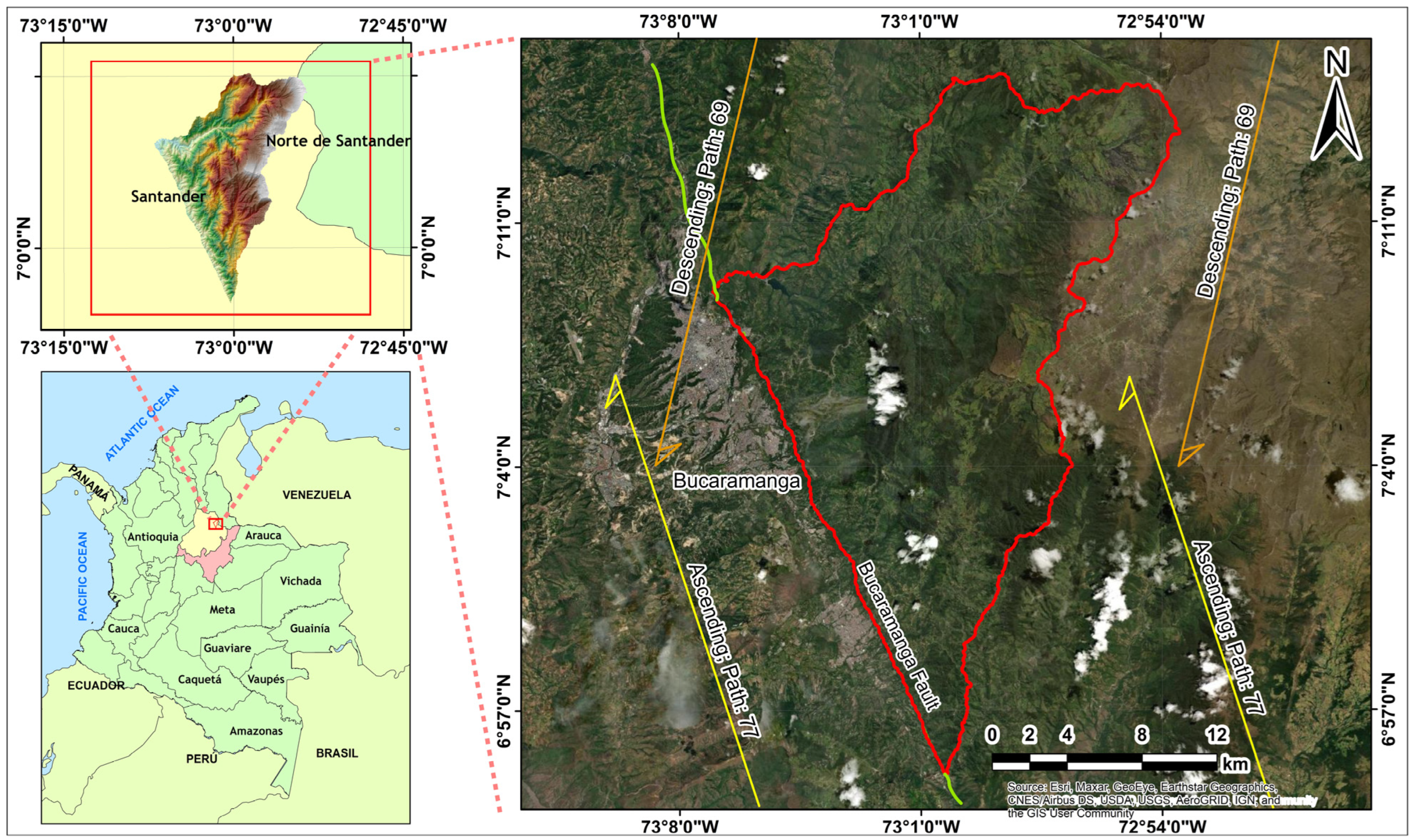
In this sense, these tectonic and structural aspects are framed in regional terms, mainly by the tectonic environment of the Bucaramanga Seismic Nest and regional faults, such as the Bucaramanga Fault, which may be creating surface deformation contrasts due to their activity. Reid [
33] put forward his mechanical model of the “Elastic Rebound”, in which it is described that the accumulation of great forces in certain preferential areas of the Earth’s crust generates increasingly greater elastic deformations of the rocks until the resistance of these rocks is exceeded, concurrently giving an almost instantaneous release of the accumulated energy; as a result, a seismic wave is generated that creates different states of deformation, giving way to the formation of fracture planes or faults, often visible on the surface. This approach is due to the fact that, in recent years, the number of mass movement events has increased in the study region, and these have generated substantial economic losses in infrastructure and also claimed human lives. At the same time, in previous studies carried out by the Colombian Geological Service (SGC), it has been described regionally that for the present region, there are conditions of high hazard due to mass movements, where rainfall and/or seismic activity are the greatest precursors [
34,
35].
3. Methods and Materials
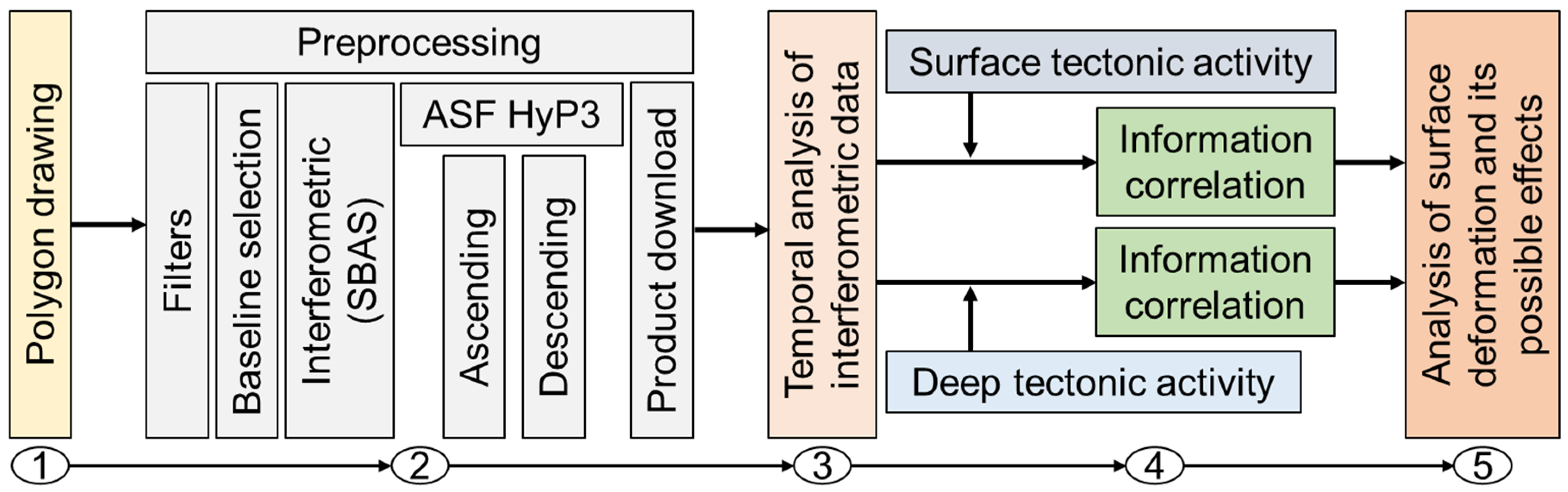
For the analysis of the degree of temporal deformation of the surfaces in the study region, and as this deformation may be related to the regional tectonic activity, a correlation is sought between the temporal analysis involving data obtained using the Synthetic Aperture Differential Interferometry (DInSAR) technique and the factors that influence this ground deformation due to the kinematics associated with the effect generated by the Seismic Nest of Bucaramanga and the Bucaramanga Fault. To this end, based on the workflow described in
Figure 2, this relationship is sought to establish points of convergence that give an idea of the terrain’s pattern of behavior. The use of DInSAR data can be a very versatile tool in the study of ground deformation conditions, as it provides the opportunity to generate an analysis regionally, with advanced satellite techniques, low costs, and a shorter data processing time [
23,
41].
To establish the relationship between these conditions following the designed workflow (
Figure 2), the first and second steps are carried out via the Alaska Satellite Facility portal [
42], in which satellite images taken over the study region are delimited, filtered, processed, and downloaded. Within these first two steps is framed the pre-processing of the satellite images provided on the ASF portal, which are part of the European Space Agency’s (ESA’s) Copernicus program and its Sentinel-1 mission, which takes images of C-band synthetic aperture radar [
43]. The selection of the images is performed by means of the classification of specific parameters based on creating a phase difference between multi-temporal pairs of Synthetic Aperture Radar (SAR) images of the same study area. This allows precision monitoring of regions that present deformations or displacements in the ground surfaces that are observed based on the record generated by the satellite’s Line-of-Sight (LOS) displacement image [
1]. Within the configuration parameters (filters) in the ASF portal, the selection polygon for the Sentinel-1 images is created, the date range is established (which for the present study is carried out in multi-temporal mode between the years 2014 and 2021), the type of image format is selected to generate the differential interferometry, Single Look Complex (L-1 SLC), Imaging Mode, Interferometric Wide Swath (IW), Polarization (Dual HH + HV, VV + VH and Single HH, VV) and Satellite Path Direction (Ascending and Descending), both of which are independently processed paths.
With the classification parameters established, a relationship between SAR images is then sought to generate a chronologically ordered pair (master and slave image), basically defined as the baseline selection for the two images. This was done in order to create differential interferometry from the selection of images by means of the Small Baseline Subset (SBAS) technique, taking advantage of the characteristics of SAR images for a short temporal and special baseline [
2,
44]. With the creation of the baseline and the selection of the ordered pair of images, the processing of these elements is carried out to obtain differential interferometry. This processing is performed using the Alaska Satellite Facility’s Hybrid Pluggable Processing Pipeline (ASF HyP3) program, which is a tool available on the ASF portal [
45,
46]. The ASF HyP3 is a free service that was developed to process synthetic aperture radar (SAR) images, benefiting users by reducing image processing where distortions are eliminated, the amount of computing resources is minimized, some program complications and usage costs are eliminated and the user is helped to manage the complexity of SAR processing [
45,
46]. The products generated under the ASF HyP3 have a spatial resolution of 40 m and are based on the Copernicus GLO-30 Digital Elevation Model (DEM), which has a native resolution of 1 arcsecond (about 30 m).
For processing in the ASF HyP3 program, the Sentinel-1 image pair is selected in the direction of the ascending and descending orbital direction. This procedure is carried out independently and in parallel thanks to the benefits provided by the support of the ASF portal, in which the processing of the images is carried out by means of a work order that is uploaded to a cloud, of which a series of internal orders (11 steps) are executed, arranged in three phases (pre-processing, InSAR processing, post-processing) [
45]. From this procedure, a total of 11 products are obtained, arranged by selection in the configuration of the processing characteristics that are executed in the work order. The products of the Coherence Map (correlation), Line-of-Sight Displacement Map (LOS) and Vertical Displacement Map are acquired for the present research.
The coherence map expresses the overlap between the two images and represents the homogeneity generated by the correlation of pixels measured between the phase of two images in a window centered on that pixel; of this overlap, the values close to 1 will have the greatest consistency [
1,
45,
46]. The Line-of-Sight Displacement Map (LOS) is a one-dimensional projection that describes the movement of the ground in meters along the display vector (line of sight) and is based on the conversion of the unwrapped differential phase, where positive values are observed as uplifts and negative values as subsidence [
23,
45,
46,
47]. The vertical displacement map is a projection from the differential phase measurements, developed under the assumption that the displacement is completely in the vertical direction by means of a mathematical transformation of the LOS displacement, and its values are expressed in the same condition as LOS [
45,
46,
48,
49].
The third step described in the methodological workflow (
Figure 2) consists of a statistical analysis based on the differential interferometry performed on each pair of Sentinel-1 images. For this analysis, a certain number of zones or areas (ratio in pixels) are taken randomly that are the most concordant among all the images resulting from interferometry as Statistical Control Points (SCP). From these control points, a correlation is made with the images to establish a time series (multi-temporal), thus describing the behavior of the degrees of deformation present in the study region [
5,
50,
51]. For this statistical analysis, the Sentinel-1 images arranged in the ASF port between the periods 2014 and 2021 are selected, where the pair of images for differential interferometry are taken at an interval of 3 months, thus generating 4 interferometry images per year. The construction of this analysis is carried out by means of a box-whisker diagram where the characteristics of time, dispersion and symmetry of the control points are described. The fourth step described in the methodological scheme comprises two phases. These phases involve the correlation and analysis of the tectonic environments (Bucaramanga Seismic Nest and the Bucaramanga Fault) and the surface displacement states in temporal terms. This analysis seeks to establish a deformation pattern of the rock massif based on the multi-temporal analysis and its correlation with regional tectonic elements. These deformation patterns, evaluated according to regional tectonic-structural aspects, can aid understanding of the dynamic behavior of surfaces as a function of the generation of instability planes as an inherent endogenous parameter. To carry out this analysis, the seismic record is taken, which is acquired by downloading historical data from the database of the Colombian Geological Service (SGC) within a radius of 200 km [
52], and centered on the city of Bucaramanga, Colombia. Seismic events recorded in a depth range between 0 and 50 km (crustal region) are also selected [
53,
54] with a Moment Magnitude (Mw) greater than 4.0. This magnitude reference is taken from the studies carried out by Keefer [
55,
56] and also the contributions generated in the studies carried out by Rodríguez et al. [
53], Papadopoulos and Plessa [
57] and Bommer and Rodríguez [
54], where a variation of the threshold defined by Keefer in terms of minimum magnitude and distance is described, and in which seismic activity can generate surface effects such as mass movements.
For the fifth step within the methodological scheme, a comprehensive analysis of the deformation factors present in the study region is carried out, examining how these factors may be influencing the generation of surface instability effects. Being able to establish this type of superficial dynamic behavior would contribute greatly to regional knowledge on this subject, providing a tool that would facilitate the construction of surface models that can provide answers during the construction of regional development plans within an anthropogenic environment. In turn, within the context of disaster risk management, they would contribute greatly to management and development plans for the protection and expansion of natural and/or anthropogenic areas, integrating specific information into studies of susceptibility and hazard of geoenvironmental risks.
4. Results
For the analysis of the degree of deformation present in the Santander rock massif in the study region, we started with the construction of the temporal sequences of differential interferometry from the Sentinel-1 images. For this construction, the study region (creation of the polygon) was delimited within the ASF portal for the selection of images in order to define the baseline and subsequently develop the SBAS technique [
2,
6]. The configuration parameters described in
Section 3, steps 1 and 2, were applied for each pair of Sentinel-1 images in its ascending and descending orbit. The selected Sentinel-1 images covered the period from 2014 to 2021, with a ratio between images (master and slave) of every three months (90 days) and a spatial resolution of 40 m. A total of 59 Sentinel-1 images were taken from the present selection, generating a total of 225 pairs for differential interferometry (111 ascending and 114 descending) [
42,
43]. The images selected for the production of the interferograms had a temporal (<90 days) and short spatial (<200 m) baseline to limit the loss of coherence between pixels [
58].
With the baseline established and the configuration parameters selected, the differential interferograms were calculated using the SBAS technique by means of the ASF HyP3 program [
45,
46]. To eliminate the topographic contribution, as mentioned in
Section 3, the ASF HyP3 program takes as its base the Copernicus GLO-30 DEM with a spatial resolution of 30 m; in turn, for the execution of the work order, a selection was made by the type of product to be obtained based on the required spatial resolution. This selection considered two types of appearance, 20 × 4 or 10 × 2, which determine the resolution and pixel spacing of the resulting images (products). The first number indicates the number of
looks in the range and the second number is the number of
looks in azimuth [
45,
46]. For the present research, the 10 × 2 appearance generated by a product with a spatial resolution of 40 m was taken, since the 20 × 4 appearance has a resolution of 80 m. The 10 × 2 appearance was taken because the generated product has a high degree of detail which can provide a greater contrast of the zones of punctual deformation over the study region, which also favors the correlation with the areas that have historically presented unstable points on the surface (mass movements).
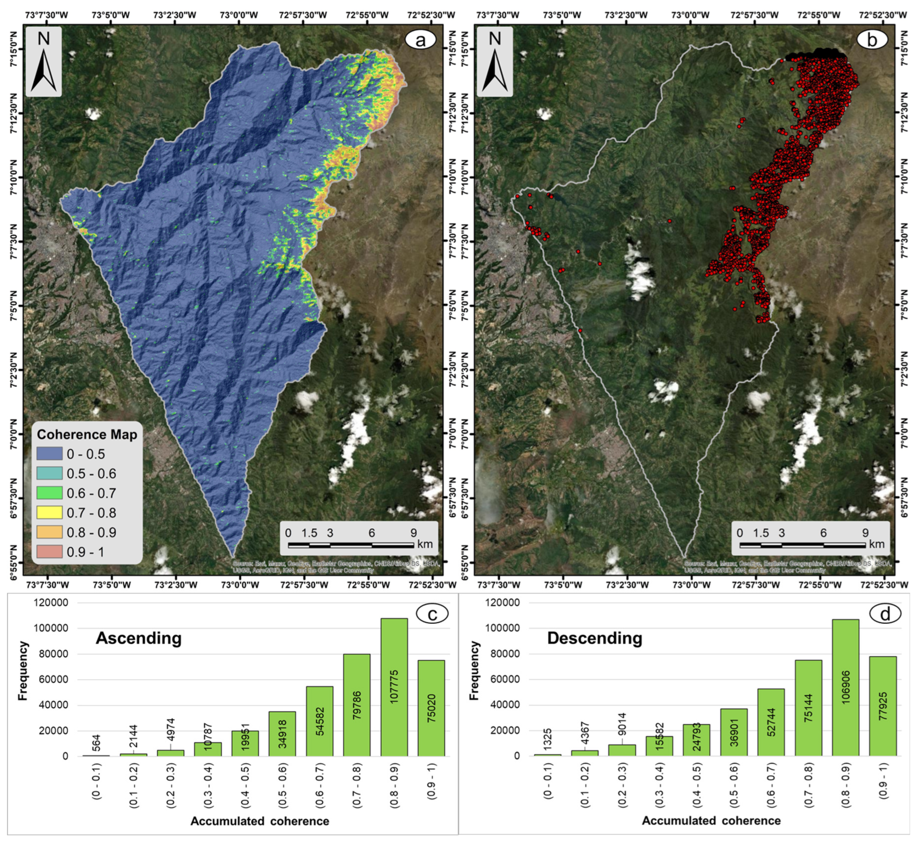
The products generated and subsequently downloaded from the ASF portal were delimited to the geometry of the study region (404 km
2), in order to perform the analysis of the deformation from the statistical control points (SCP), followed by the correlation with the catalog of seismic events associated with each tectonic geometry. The first product obtained corresponded to the coherence map, which was an important basis for the following analyses, since this product determines the degree of correlation between the pair of processed SAR images. The coherence threshold used was ≥0.5 (medium to high
multilook factor) for the present research. From this threshold, an average of 24,105 coherent pixels out of 252,377 was described for the entire study region between the ascending-orbiting interferograms and 19,930 coherent pixels for the descending-orbiting interferograms (
Figure 3a).
To perform the statistical analysis, a sample size of 3550 SCP was taken for interferograms in ascending orbit and the same for the descending orbit; this selection was made randomly (
Figure 3b). From the correlation of the SCP with each interferogram in ascending orbit, it is described that, for the range between 0.7 and 1, there is a number of 67.2% of coherent accumulated pixels (
Figure 3c), and for interferograms in descending orbit at that threshold, 64.2% of coherent cumulative pixels are present (
Figure 3d). At the same time, it is observed that the number of pixels with a good correlation with reference to the total area of study is very low, in a ratio of 1:10 (approx. 10%); therefore, the points that were generated as SCP were taken as evaluation points for the analysis of the Line-of-Sight Displacement Map (LOS) and the vertical displacement map. This aspect is important to highlight, since, as can be seen in
Figure 3a, for the total area of the study region, 90% of pixels show low coherence (≤0.5). This is largely due to the effect generated by the areas that have dense vegetation cover 48% (194 km
2) of the study region.
Vegetation is one of the factors that generates a volumetric dispersion effect within the interferogram, showing low coherence values that are described as areas that contain only noise, since significant vegetation cover reduces the spatial density of the coherent elements [
8,
25]. The effect of vegetation is described due to its high presence in the region, since it was possible to identify forested areas from an analysis that considers the minimum canopy density of 30% and minimum canopy height in situ of 5 m, with a minimum area of 0.01 km
2. This information was acquired through satellite monitoring of forest areas carried out by the Institute of Hydrology, Meteorology and Environmental Studies (IDEAM), based on medium- and high-resolution images from Sentinel 1–2 and Planet Scope [
59]. The other factor influencing the low coherence for the region is the topographic slope relationship. If we take as a reference the areas that have a slope > 30°, they represent 34% (137 km
2) of the study area, to which condition is added the geomorphological aspect, which is described as an abrupt relief with straight and steep slopes. This effect of topography on the coherence of short baseline interferograms is very important, as areas with steep relief or a high slope often induce important atmospheric signals [
8,
24].
Considering the above, the objective of this research is to estimate the degree of deformation of the rock massif in the study region influenced by the tectonic elements present, and as an added value, how this deformation can inherently affect the creation of unstable planes. To this end, the regions that present a high coherence within the interferograms are selected, in addition to the selection of the SCP as internally distributed points that are found in the regions that have a relatively flat, homogeneous topography of great extension and with a low density of vegetation (forests). They were considered because regions with arid terrain or little vegetation, and with homogeneous and flat surfaces, can obtain high values of temporal coherence [
1,
60]. This allows a coherent evaluation to be made for the degree of analysis required in the present research, where the physical concept was also applied that the rock massif for the study region behaves as a rigid body that is limited by the regional tectonic and structural context. In this way, the average degree of deformation is established for the entire study region with some subtle internal variations.
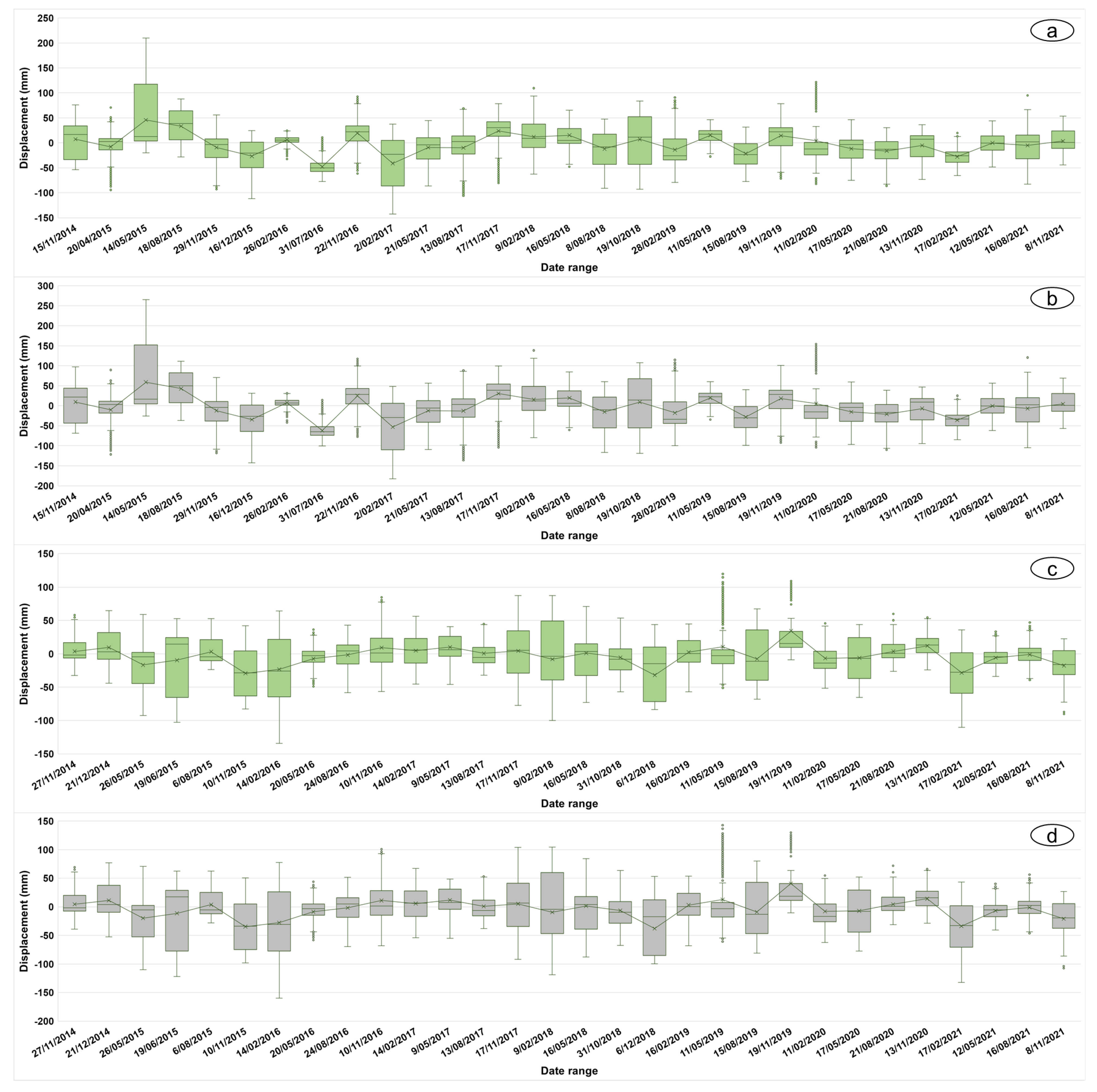
Within the statistical analysis, as a function of differential interferometry (step 3,
Figure 2), the construction of the multi-temporal statistical sequence of each differential interferogram in ascending and descending orbit was carried out, where the Line-of-Sight Displacement Map (LOS) and the vertical displacement map products were downloaded, which were correlated with the SCP. These products were obtained under the work order carried out on the ASF portal and were later delimited to the geometry of the study region. The correlation of the SCP with each of the differential interferograms was performed independently for the LOS and vertical (ascending and descending) images, and from this, a box-whisker diagram was constructed, obtaining four multi-temporal sequences that will be shown later. The degree of deformation present in the study region, described by the relationship between the SCP and the differential interferograms between the years 2014 and 2021, is shown in
Figure 4; here, we can see the behavior of the displacement of LOS in
Figure 4a, and in
Figure 4b, the transformation to the vertical, and observe these two sequences in the ascending direction of the satellite. The sequences described in
Figure 4a,b show the same trend, but the vertical displacement has a slight increase with respect to LOS. Since the vertical displacement is the transformation of LOS, the maximums and minimums generated on the analyzed region are described [
49].
For these two sequences, a maximum (uplift) displacement in the vertical of 151.7 mm (117.5 mm in LOS) and a minimum (subsidence) of −110.2 mm (−86.2 mm in LOS) are found. Looking at the complete sequence, between the years 2014 and 2017 the highest rates of deformation are described. Subsequently, a somewhat homogeneous and stable behavior is observed, with an oscillating trend giving an elastic rebound effect that remains in the system at a low magnitude for the subsequent years. On the other hand, in
Figure 4c, we can observe the displacement behavior of LOS and in
Figure 4d, the transformation to the vertical in the descending direction of the satellite. These two multi-temporal sequences have a maximum vertical deformation of 59.7 mm (49.3 mm in LOS) and a minimum of −85 mm (−71.5 mm in LOS) present in 2018. The general behavior of these two sequences differs with respect to
Figure 4a,b; this is due in part to the position of the satellite (ascending and descending) and the antenna receiving the backscattered signal, which may be affected by the orbital phase, angle of intake or geometric condition of the medium [
1]. The latter, with reference to the orientation and slope of the surfaces of the study region, added to a possible change in the direction of displacement created by seismic activity and the motion tensor, which describes the geometry of the faulted plane in a two-dimensional way and its movement, the latter of which will be evaluated below. The sequence in general manifests the same singularity as the ascending sequence, with an oscillatory effect of low magnitude.
For the analysis of the deformation sequences correlated with the seismic events present in the study region, we first want to clarify that this analysis was approached from a temporal perspective between these two aspects. The objective is to determine the influence of seismic activity as a surface deformation element within the pair of processed SAR images, especially for the co-seismic deformation generated by an earthquake [
7,
61]. For this analysis, the information reported by the Colombian Geological Survey (SGC) was used, in which a record of 86,817 seismic events was obtained for the period between 2014 and 2021 [
62]. These events were selected with the parameters of depth (<300 km), magnitude (≥1 Mw) and a radius of 200 km (center in Bucaramanga). A filter was made for this catalog where events with a depth between 0 and 50 km, magnitude ≥ 4 Mw and a radius of 200 km were selected, producing a total of 17 seismic events with these characteristics, whose horizontal distance with respect to the study region was calculated (
Table 1). The other events present in the selection will be discussed in greater detail in the next chapter with reference to their participation in the degrees of deformation.
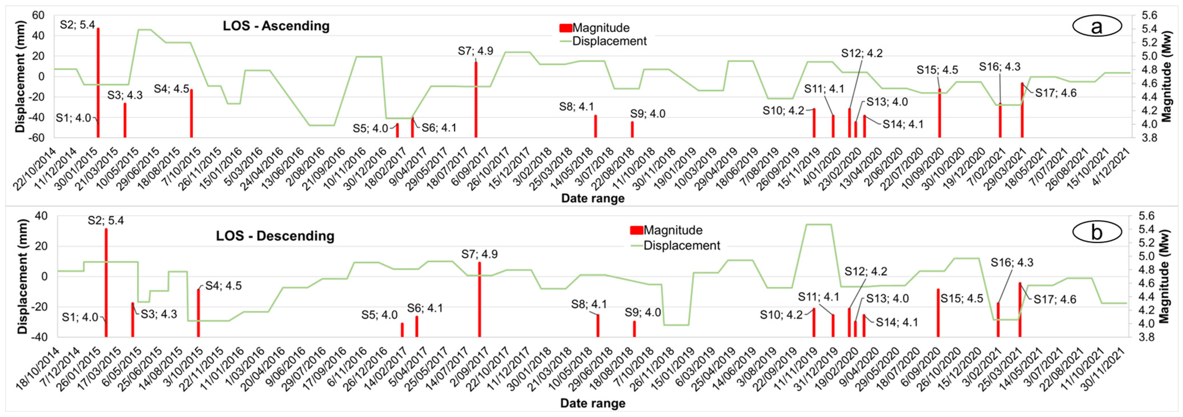
For the present analysis, the 50th percentile that is part of the analysis of the SCP (0.7–1) of the previously generated statistical construction of each differential interferometric pair was taken, and this was correlated with the inventory of selected seismic events. The purpose of this correlation is to observe whether the seismic event had an impact on the deformation of the ground, and in what type of phase, but it does not fully describe the rate of displacement. This is due to the separation applied for the interferometric process of the images (3 months), which is not directly correlated with the date of the seismic event. This condition only provides information on the present correlation between cause and effect but does not fully establish the displacement rate in the factor of magnitude, since this requires a more detailed analysis that considers each seismic event separately. For ascending LOS interferograms of the satellite (
Figure 5a), it is observed that registers S7, S8, S10, S11 and S17 (
Table 1), contrasted with the generated deformation line, create a positive displacement phase (uplift) due to the co-seismic effects generated. Based on the present correlation, aspects that differ between each sequence can be observed (
Figure 5a,b).
An important aspect to note at this point is the relationship proposed by Massonnet and Feigl [
7], with respect to the deformation patterns observable within the interferogram, since earthquakes of a magnitude M > 5 and with a depth of <10 km can generate clear stripe patterns. According to this, the S7 event would be concordant with these conditions, but observing the deformation line, its impact on the study region was slight. This is due to the distance between the event (epicenter) and the study region, which has a length of 96.7 km, which is why the degree of deformation as a zonation decreases as it moves away from the epicentral site, as can be seen in the works of Hashimoto et al. [
63] and Ganas et al. [
64]. In turn, this event is associated with the stroke of the Guaicáramo Fault (kinematics reverse-dextral), which is an active fault with a moderate activity rate (0.1–1 mm/year) [
65]. In addition to the above, events S8 and S17 present a positive phase, but their depths (21 and 30 km respectively) are not concordant with what was proposed. For the satellite’s LOS interferograms descending (
Figure 5b), it is observed that registers S1, S2, S3, S8, S10, S11, S15 and S17 (
Table 1) have a positive displacement phase (uplift) due to the co-seismic effects generated. Of these events, only S2 would be consistent with what was proposed by Massonnet and Feigl [
7]; the others differ in one condition or another. Events S4, S5, S6, S9, S12, S13, S14 and S16 differ in some parameters from those proposed; in addition, their geometry is seen in a negative displacement phase (subsidence). On the other hand, event S5 is associated with the stroke of the Suarez Fault (kinematics reverse-sinistral), which is an active fault with a low (0.01–0.1 mm/year) to moderate (0.1–1 mm/year) activity rate [
65]. The S13 event is associated with the stroke of the La Salina Fault (inverse kinematics), which is an active fault with a low (0.01–0.1 mm/year) to moderate (0.1–1 mm/year) activity rate [
65], and events S10, S11, S12, S14 and S15 are associated with the stroke of the Bucaramanga Fault (kinematics reverse-sinistral), which is an active fault with a moderate (0.1–1 mm/year) to high (1–10 mm/year) activity rate [
65].
As mentioned above, there is a significant discrepancy between the deformation rates observed by the ascending and descending view of LOS and their correlation with seismic events. This behavior is largely due to the acquisition geometry and the sensitivity of the signal due to the effect of the displacement of the satellite, which is limited only to measuring the movement of the ground in a one-dimensional (1D) way in the field of view of LOS, thus acquiring the displacements due to the co-seismic effects in an anamorphic way and with biased source parameters [
66,
67]. The other factor that influences the behavior of
Figure 5a,b, especially where it correlates with the events of
Table 1, is the effect of the focal mechanism, since it describes in a two-dimensional way the geometry of the fault plane and its motion. An important aspect to mention within the general behavior of
Figure 5a,b, is that these are the sectors that do not have a point of convergence with the seismic record, since it is not possible to establish the reason for the present deformation. Among these sectors is the behavior, especially in 2016 and 2019, in an ascending and descending direction, which, in turn, relatively describe the highest rates of deformation without a seismic event that presents the aforementioned characteristics. Taking this into account and adding other sectors that present the same conditions, the surface seismic events, as described, would not generate the present surface deformation. Based on this, for the present research and taking into account the results obtained from the superficial analysis, which are based on the descriptions made by Massonnet and Feigl [
7], temporal spaces are observed within the sequence of differential interferometry images that do not present a convergence with this surface tectonic analysis. In this sense, in order to establish a broader assessment where a scenario that generates these disturbances is proposed, an assessment from a more regional point of view will be addressed.
With this approach, it is observed that the study region is located at the interaction of three tectonic plates (Nazca, Caribbean and South American Plate) that generate at the level of the Colombian territory zones that are described in the study by Chen et al. [
68] as subduction, stable continental region (non-Craton) and active continental shallow region, the latter being the area where the study region is located. Within the active continental shallow region, there is a particular feature belonging to the tectonic environments, defined by Taboada et al. [
69,
70] and named as the “Seismic Nest of Bucaramanga”, a term used for the first time by Tetsuo Santo in 1969 (cited in Prieto et al. [
71]) that refers to a large number of intermediate-depth seismic events present in the Bucaramanga region; this reference also alludes to the definition proposed by Richter [
72], in which he defines the sectors with a large number of seismic events worldwide as a “Seismic Nest”. This tectonic aspect distinguishes the Bucaramanga Seismic Nest due to its large number of seismic events with magnitudes between 4 and 5 (Mw) and depths between 140 and 200 km [
71].
The present tectonic context arises for the study region due to its proximity, and also due to its large amount of seismic activity. Taking into account the analysis generated by Valencia Ortiz et al. [
32], in which an estimate of the seismic productivity generated by the Bucaramanga Seismic Nest is made from a catalog of events between the years 1993 and 2021, it is observed that, for the region, a total of 524 events of magnitude 3 Mw, 42 events of magnitude 4 Mw and three events of magnitude 5 Mw can be generated per year. From this analysis and considering the seismic events that were not previously selected, a further evaluation was carried out, selecting the events of magnitude ≥5 Mw and depth >50 km (
Table 2). From the present selection, a total of 17 seismic events were found, which were correlated with the multi-temporal sequences of the differential interferograms of LOS-ascending and LOS-descending created by the 50th percentile. From the present correlation, a high convergence of the dates of seismic activity is observed with the regions that presented temporal spaces where the action of an element that generated the present surface deformation was not evident.
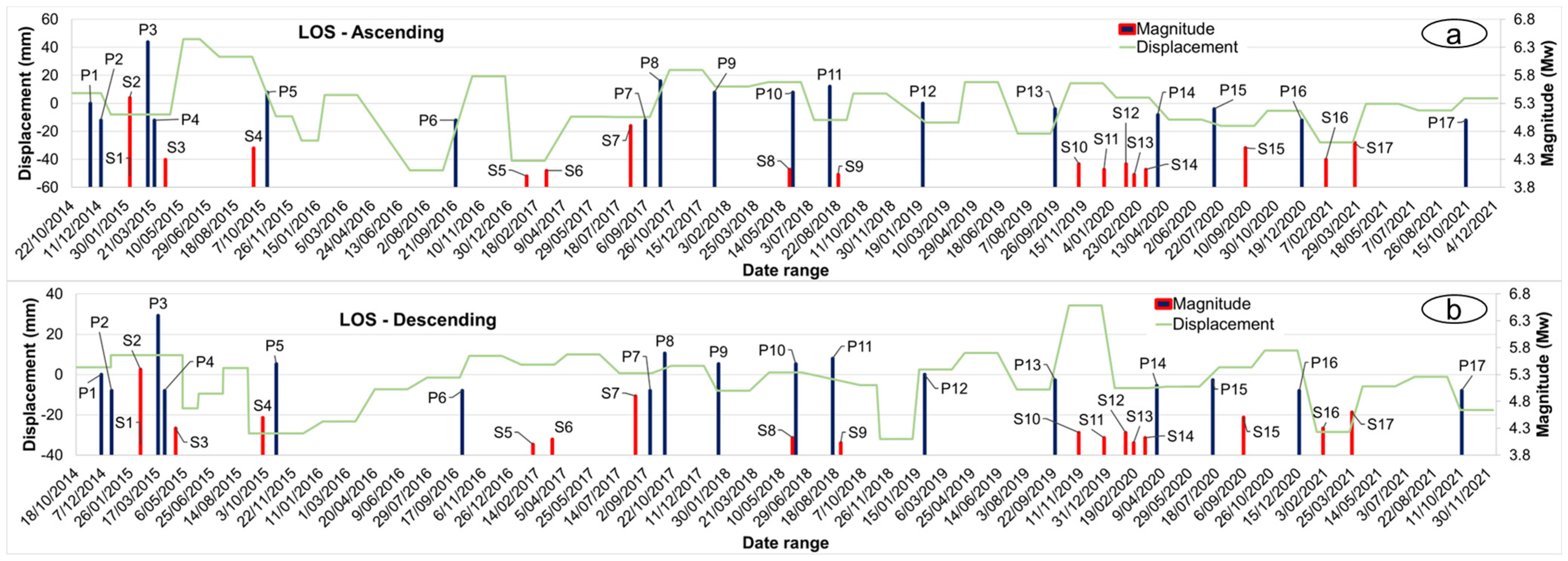
For the multi-temporal sequence on the line LOS-ascending (
Figure 6a), it is observed that the seismic events P3, P4, P5, P9, P11, P12, P14, P15 and P16 (
Table 2) describe a negative phase (subsidence) due to the co-seismic effects generated. These events have an average depth of 148 km, with an average horizontal distance to the study region of 26 km, which would be found in the tectonic environment of the Seismic Nest of Bucaramanga. An aspect of these events that it is important to describe is their shape, which is evidenced in a subsidence phase a condition that would be framed to a greater extent by the type of focal mechanism which describes the geometry of the fault and its movement, the latter being important for its relationship with the field of view in the satellite’s trajectory; these aspects will be evaluated later.
Events P1, P2, P6, P7, P8, P10, P13 and P17 describe a positive phase (uplift). For the multi-temporal sequence on the line LOS-descending (
Figure 6b), it is observed that the seismic events P1, P2, P5, P7, P9, P11, P14, P16 and P17 (
Table 2) describe a subsidence phase, and are found at an average depth of 148 km and an average horizontal distance of 26 km (except for P2, which is 182 km), which condition places them on the Seismic Nest of Bucaramanga.
Events P5, P9, P11 and P14 are observed in both satellite trajectories due to the type of motion (focal mechanism), and events P1, P2, P3 and P4, which present an inverted phase in
Figure 6a,b, display a condition also associated with the focal mechanism and the way of observing the satellite trajectory. From the present analysis, it is observed that the seismic events are not concordant with what was described by Massonnet and Feigl [
7] in relation to the magnitude and depth; however, if we take into account what has been observed from the behavior of the graph (
Figure 6), in addition to a degree of magnitude that is greater than 5 Mw, the seismic productivity, the proximity of the events, the tectonic environment and the type of rock (which would have a better response in the propagation of the energy released by the seismic event), a high correspondence between the degrees of surface deformation and the deep seismic events present in the study region is obtained. However, unlike surface events, these would generate subtle changes in the surface deformation that would occur within a range of ±20 mm (data calculated from the values of the interferograms only where they correlate with the deep events).
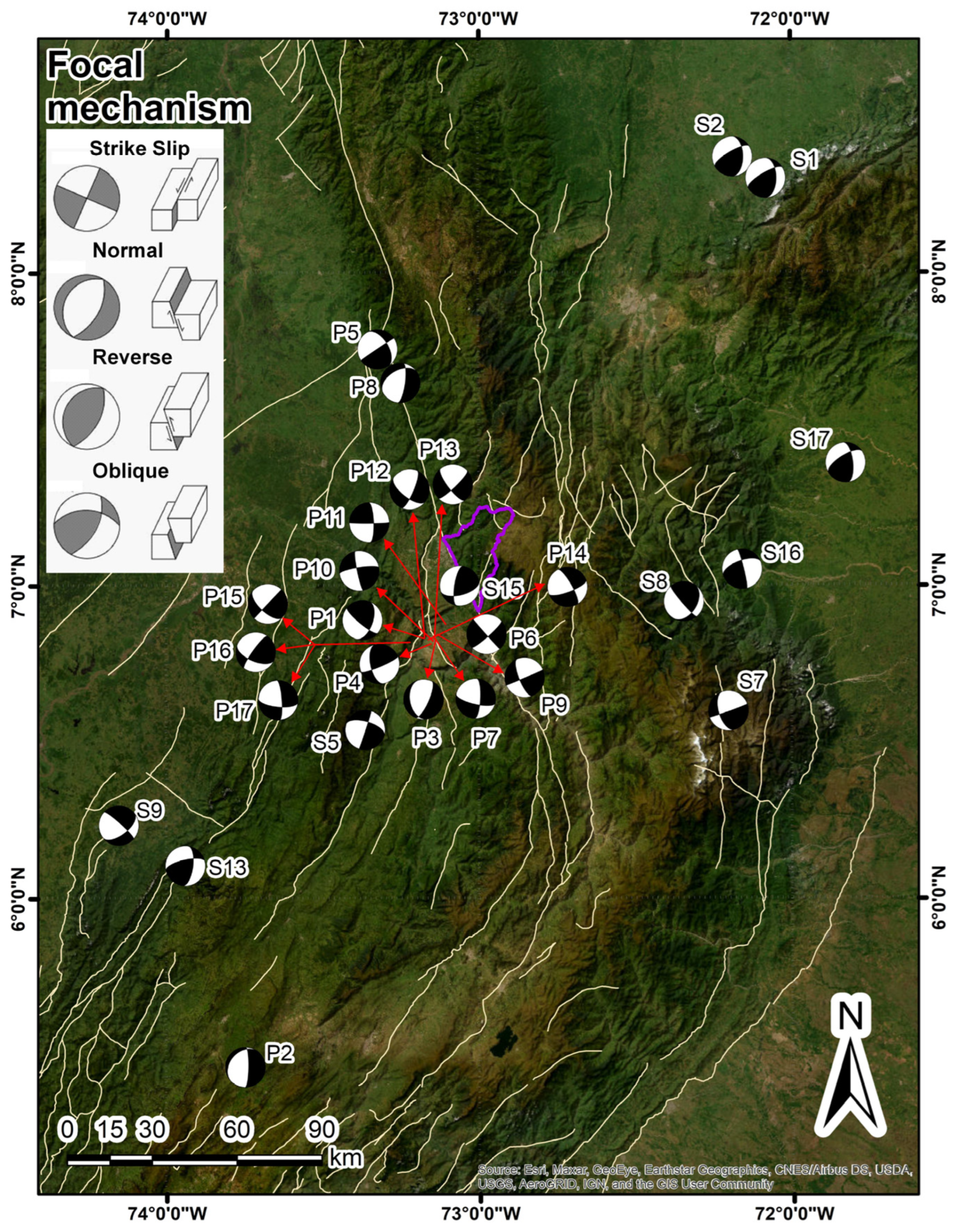
On the other hand, performing the analysis of the focal mechanisms generated from the seismic record of each event, this clear correspondence of the shape of the graph in its subsidence and uplift phases is observed, which, in turn, is also influenced by the field of view of the satellite trajectory. The focal mechanism shows the geometry and movement of the fault described from the proposed solution to determine a behavior of compression (reverse fault), expansion (normal fault), transformation (strike slip fault) or combined (oblique fault). In this context, punctually, for the trajectory of LOS-ascending in positive phase (uplift), the events P1, P7, P13, P17, S8 and S17 (oblique) are concordant with the degree of deformation on the surface, and the events P3 (normal), P9, P11 and S5 (strike slip) and P4, P5, P14, P15, P16, S1, S2, S7, S9, S13, S15 and S16 (oblique) agree with the negative phase (subsidence) (
Figure 7). For the trajectory of LOS-descending in positive phase, events P4, P12, P13, P15, S1, S2, S7, S15 and S17 (oblique), S8 (reverse), and in negative phase, events P1, P5, P7, P14, P16, P17, S9, S13 and S16 (oblique), P9, P11 and S5 (strike slip) and P2 (normal) are concordant with the degree of surface deformation. We want to make it clear that, due to the strike plane described by the strike and oblique focal mechanism, these can occur in both the directions of LOS-ascending and descending.
In order to establish a correct correspondence of the focal mechanisms of the surface (S) type, an association was made with the structural styles described on the surface as a reference point between the type of seismic activity, the tectonic and/or structural environment and the manifestation of the type of deformation on the surface (positive or negative). At the same time, for the focal mechanisms of the deep (P) type, based on their description in location and geometry, they were located on the tectonic environment in which this seismic activity would be generated (
Table 3). From this correlation, the source that generates the seismic activity and the effects generated on the surface are coherently established, providing reliable support to support the cause/effect conjecture.
However, on the graph (
Figure 6), there are still sectors that do not correlate with a seismic event generated from the two selections made (surface and deep). In this sense, the option of smaller magnitude events (4 to 5 Mw) that could have an impact on surface deformation conditions was explored. To do this, the range of dates that did not present a seismic event was taken as a basis and on this basis, a seismic event with the highest reported magnitude and that presented a focal mechanism according to the deformation generated was sought (
Table 4).
From this analysis a new research question is generated: To what extent can deep seismic events have an impact on the degrees of deformation on the surface? A solution to this question could be posed by the acquisition of data of greater precision than those described by the analysis of satellite observations. This data acquisition can be given by a direct measurement on the evaluated surfaces in this case, on the rock massif (Santander Massif), which through the installation of a Global Navigation Satellite System (GNSS) would have real-time data in the three coordinates for the moment of seismic wave generation. With this information, a more concrete answer could be given about the low-magnitude (Mw ≤ 5) deep seismic activity that may be generating surface deformation effects. In the same way, without considering the above, a great correspondence between seismic activity and the degrees of surface deformation is observed for the present study. This activity is directly proportional between the cause that is generated by the seismic event and its effect, which is described by the deformation created, considering that this deformation has variables that depend on the magnitude of the event, depth, focal mechanism, and horizontal distance, which are conditions that define the rate of displacement.
As a final part of the proposed methodological scheme (step 5,
Figure 2), a comprehensive analysis of the deformation conditions generated by tectonic activity present in the study region and its possible influence on the generation of instability planes was carried out. From the present analysis, it is observed that seismic events have an impact on most of the conditions of ground deformation, giving rise to successive sequences of uplift and subsidence that affect to some degree the stability of the rock massif. This repetitive effect can create stress on the rocks, leading to the formation of planes of weakness that can manifest as micro-cracks or fractures in the rock [
77], which are mostly of the igneous and metamorphic type. These conditions of maximum deformation could lead to a collapse of a structure or slope (mass movement), but as observed in the multi-temporal sequences correlated with the historical planes of instability, there is no direct action between cause and effect. However, this does not exclude their participation, since a considerable increase in unstable planes (mass movements) is also observed within these sequences after the generation of the maximum deformations. The effect generated by the deformation of the ground would remain in the system as an inherent action that is later sponsored by the action of a trigger such as rains or an earthquake, the latter of which is line with the characteristics described by Keefer [
56]. For this reason, the construction of the multi-temporal sequences of the differential interferograms provides to a large extent a tool that can establish this behavior of the terrain, obtaining a certain degree of prediction in the future as a response to unstable future planes, allowing time to carry out a correct implementation within the early warning schemes, since being able to observe the degree of deformation of the terrain in a temporal way can provide a preemptive warning about sectors that show considerable variation in the degree of deformation of surfaces.
5. Discussion
As described earlier in the results chapter, both surface and deep tectonic activity have generated significant changes in surface deformation states. These states of deformation in the analyzed period (2014–2021) have an important impact on the stress generated on the rocks, leading to the creation of possible planes of weakness that are an important point within an inherent scheme of the surfaces; they can subsequently lead to the generation of events such as mass movements, which can be triggered by climatic or seismic conditions, or even by anthropic factors. These states of deformation provide basic arguments in the construction of scenarios for the evaluation of these unstable conditions on surfaces (mass movements), as these conditions are measurable in the first place by the inherent relationships that develop between the attributes and their variables such as geology, geomorphology, land cover and land use that model this spatial behavior or susceptibility [
78,
79,
80,
81,
82]. Then, the factors that trigger mass movements can be integrated into these conditions of susceptibility, changing the analysis to a spatiotemporal or hazard aspect, where intense rains, rapid snowmelt, changes in water levels, volcanic eruptions or strong shaking of the ground by the action of an earthquake are the major precursors [
83], and within these scenarios, rainfall and seismic activity are the most recurrent factors for conditions that pose the threat of mass movement [
29,
80,
82,
84].
In this context, the evaluation of each inherent element gives added value in the analysis of the conditions that can generate an alteration within that surface dynamic. To this end, one way to observe this, which can be framed as a geomorphological variable, is the degree of surface deformation measured by the analysis of satellite images; this is a tool that provides a valuable opportunity to establish this behavior of the terrain, since it allows measurements to be made indirectly, but with positive feedback on the sequential analysis generated in real time. To paraphrase Hanssen [
1], a way to analyze the deformation conditions induced by endogenous or anthropic elements on surfaces at a local scale is through observation with geodetic methods, where constant measurements can be made of high precision and with a very good spatial resolution, from which tools can be obtained that serve as an input for the analysis of environmental risk management focused on climate change, the management of natural resources, and territorial planning.
In this sense, a relationship with the historical record of generated instability events is integrated as an analysis for the present research, which events correlated with the multi-temporal sequence of surface deformation and regional tectonic activity. To this end, it is assumed that the objective of this analysis is not to estimate the velocity and displacement rates of the unstable areas present in the study region, but to generate a description of the type of event based on the criteria generated by Cruden and Varnes [
85], where a classification of the different types of movements and their relative displacement is made. The mass movements present for the region are part of the classification of fast surface movements, which is an important factor, since this type of mass movement within the interferometer differential analysis does not generate an optimal response, tending to underestimate the rate of velocity [
1,
86].
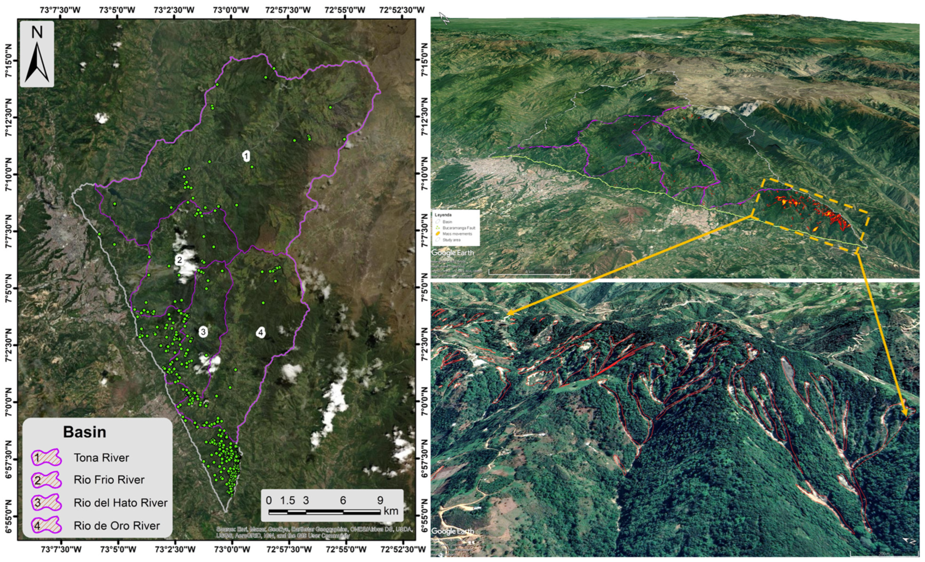
For this analysis, an inventory of mass movements was first constructed, following the classification made by Varnes [
87], where the parameters of type of movement, size and date of the movement are defined, this last parameter being the most important for the temporal correlation of the movements with the images generated from the differential interferometry. For the generation of this inventory of mass movements, data registered in international and national databases were acquired, such as the Disaster Information Management System (DesInventar), the Mass Movement Information System (SIMMA) of the Colombian Geological Service and the National Unit for Disaster Risk Management (UNGRD). Parallel to this work, a geometric construction of the undocumented movements is carried out by means of a process of photointerpretation carried out on images arranged on the Google Earth
® platform [
88,
89]. Each of the mass movements is assigned the date of occurrence of the event based on the information recorded in the databases of DesInventar, SIMMA and UNGRD, in addition to the information reported by sources such as newspapers and regional news [
84].
The data obtained from international and national sources show a total of 99 events, of these, 10 events belong to the DesInventar portal [
90], eight events on the UNGRD portal [
91] and 81 events on the SIMMA portal [
92]. A total of 269 events were obtained from the photo-interpretation process carried out on the images available on the Google Earth
® platform. Integrating each of these inventories, a total of 368 mass movements were obtained, which were characterized based on the classification made by Varnes [
87], and were grouped according to speed type [
85]. The 368 mass movements have a total area of 0.784 km
2 (0.19% of the study area) and were classified as: translational debris landslide with 131 events with an area of 0.42 km
2 (52.5% of the total event area), translational earth landslide with 146 events and an area of 0.126 km
2 (16%), debris flow with 31 events and an area of 0.098 km
2 (12.5%) and earth flow with 60 events and an area of 0.149 km
2 (19%). These events have a maximum area of 49,903 m
2 and a minimum area of 33.5 m
2. In turn, 206 events (0.275 km
2, 34%) are shallow and 162 events (0.518 km
2, 66%) are deep (>2 m thick), and are all classified within the fast-moving events (
Table 5 and
Figure 8).
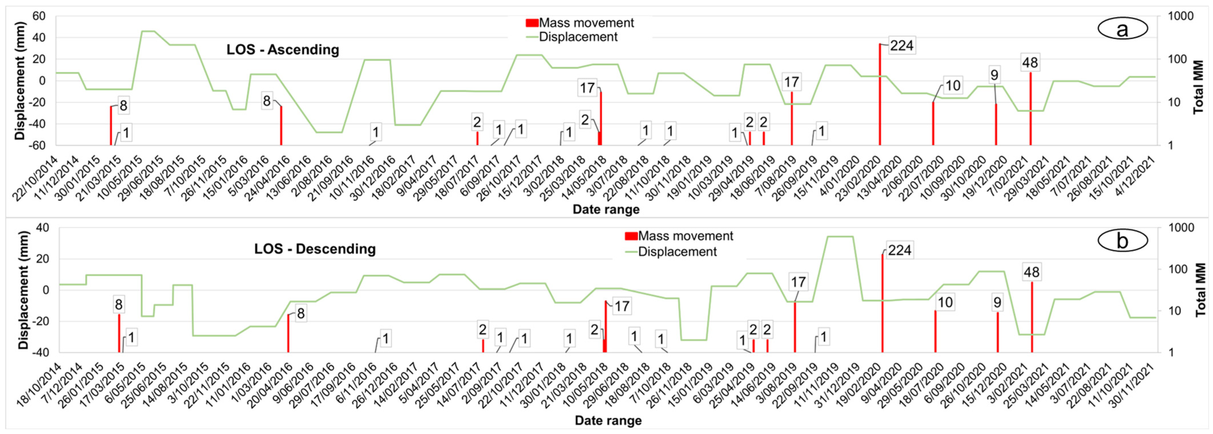
The inventory of mass movements is correlated with the multi-temporal sequences of the differential interferograms of LOS-ascending and LOS-descending created by the 50th percentile. This is because, under these conditions, the most favorable scenarios for the creation of planes of instability would occur. In addition to this, the relationships generated in the study by Valencia Ortiz and Martínez-Graña [
84] were also taken into consideration for the present analysis, with reference to seismic events that trigger mass movements (
Figure 9). From this it is observed that there are no points of convergence between seismic activity and the generation of mass movements, but a state of change in the rate of displacement and the subsequent generation of a mass movement is observed. However, the lack of connection between cause and effect is more dependent on an inherent action of the surface planes that have been destabilized by vertical displacement and that are subsequently activated or detonated by the action of rainfall or seismic activity itself. A reflection of this is the considerable and repetitive increase in mass movements generated subsequently, as can be seen in
Table 6, where the total displacement generated from an initial state prior to the date of mass movement and the current state, where it is in motion, was estimated. Furthermore, in
Table 6, the displacement phase in which the movement was generated (uplift or subsidence) can be seen.
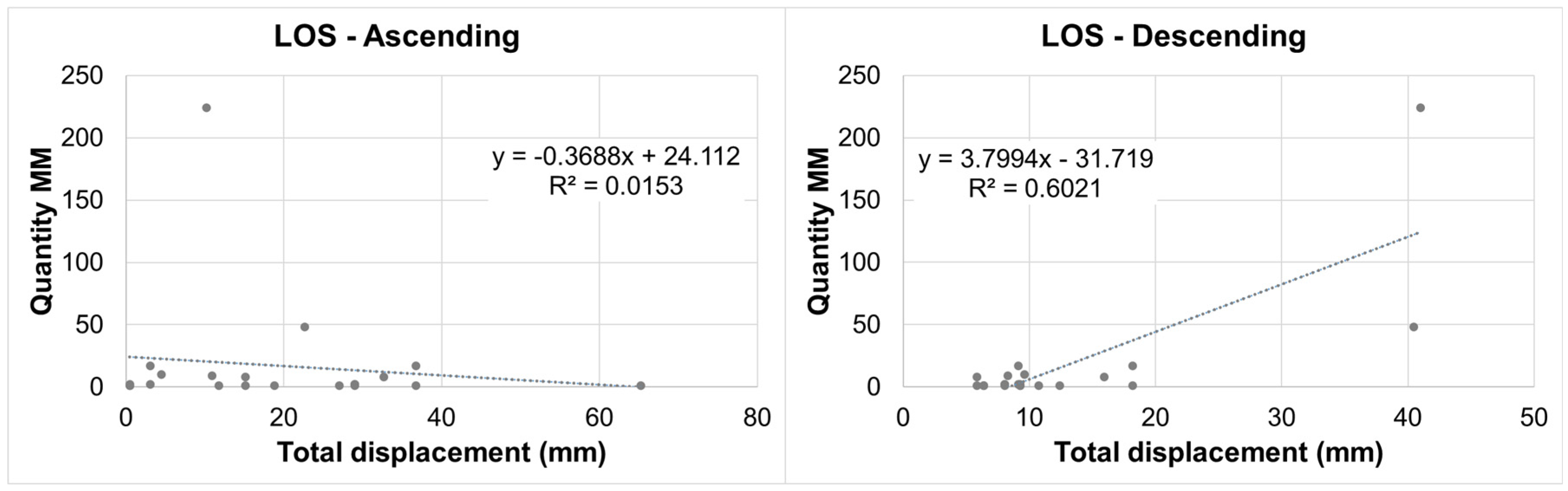
These oscillatory states generate volumetric changes of the surfaces, giving rise to a phase of disturbance of the system (rock massif) that is affected, reducing the resistance of the rocks, which are mostly crystalline (igneous and metamorphic), thus creating planes of weakness that are later exploited by the action of a trigger. In addition to the above, if we take only the sequences of the interferograms that correlate with the dates of the movements, two important aspects are observed. On the one hand, the correlation between the number of events and the total displacement in LOS-descending describes an almost linear trend (
Figure 10). This relationship can establish a recurrence of a mass movement as a function of the rate of displacement, clarifying that the number of possible events that can be generated cannot be predicted with this function. At the same time, it is observed that the largest number of movements is associated with a subsidence phase, where the predominant structural style is of the oblique type associated with the Bucaramanga fault and the Bucaramanga Seismic Nest, as described earlier in the results chapter. For the correlation in LOS-ascending, this linear relationship is not observed, which may be associated with the shape of the field of view of the satellite trajectory and the geometry of the fault plane, especially the stroke of the Bucaramanga fault that is almost parallel to this field of view an aspect that was described in the results chapter (
Figure 10). On the other hand, it is generally observed that the average deformation rates are between 18.2 mm and −21.1 mm for LOS-ascending and 13.9 mm and −21 mm for LOS-descending. All these behaviors can be measurement indicators for future events in a real-time tracking of surface deformations.
The action of the behavior of surface deformation as a trigger for mass movements would be framed as an inherent element of great weight in the analysis of susceptibility conditions, since it describes the response of surfaces and how they are disturbed (tension stress) by constant changes in deformation. On the other hand, structural control also plays an important role within the degrees of deformation, if observed by the effect generated by the stroke of the Bucaramanga fault. Since this fault is an oblique structure with a sinistral strike slip and reverse dip in the NNW-SSE direction, which, as described by Valencia Ortiz et al. [
32], generates a tilt with its activity that infers on the geometry of the hydrographic basins present on its stroke, it thus generates a tilt (asymmetry factor) in the direction of the kinematics of the fault. All these considerations within the study of susceptibility to mass movements guarantee a more complete analysis based on the variables contemplated that are directly related to the conditioning action of a mass movement, which guarantees the creation of a model more in line with the situation present in the environment [
31,
82]. Finally, it is important to mention an aspect of the study carried out by Valencia Ortiz et al. [
84], which describes how seismic activity and rainfall are relevant factors that act as a trigger for mass movements for the study region. This study established a combined effect between seismic activity (Mw ≥ 4) and rainfall, with a threshold of 53 mm for 24-h rainfall and 158 mm for accumulated rainfall from the previous 15 days in a 25-year return period, thus giving a spatiotemporally framed scenario.


 ,
, 


