
Uncertainty Quantification of Soil Organic Carbon Estimation from Remote Sensing Data with Conformal Prediction
 , ,
, ,  and
and
Abstract
: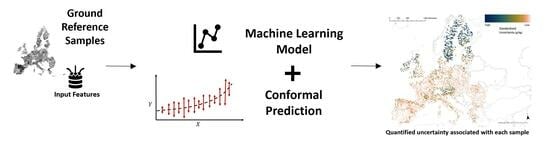
1. Introduction
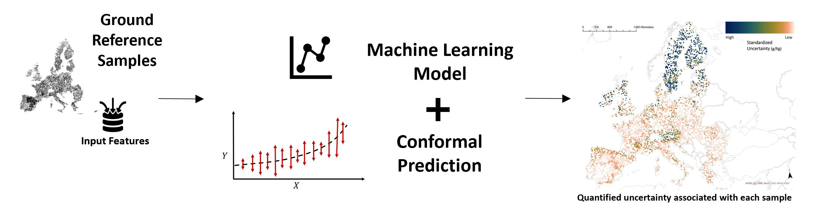
2. Mathematical Background
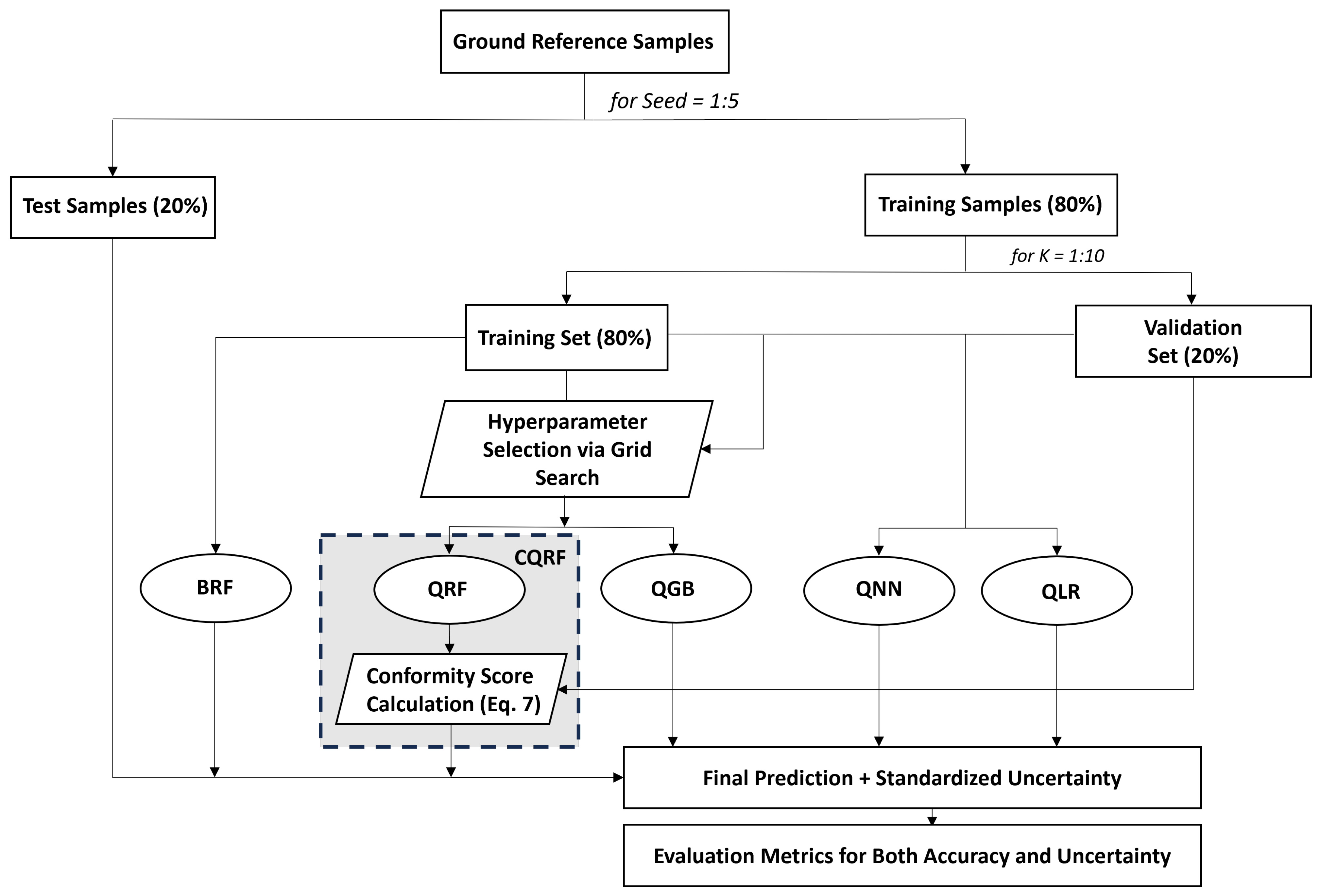
3. Materials and Methodology
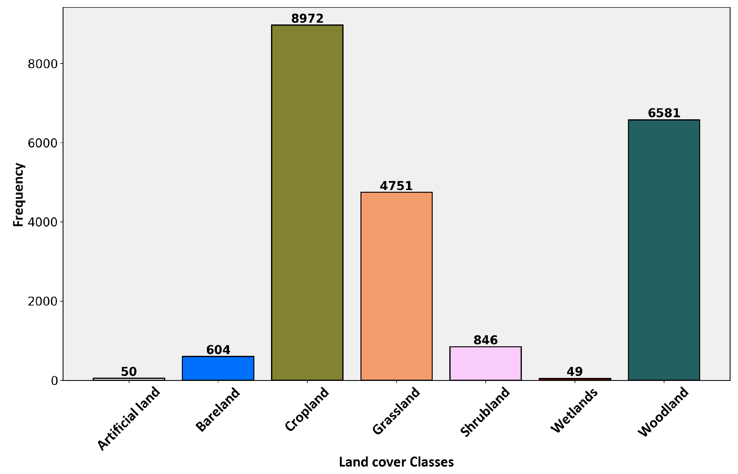
3.1. Data Description and Preprocessing
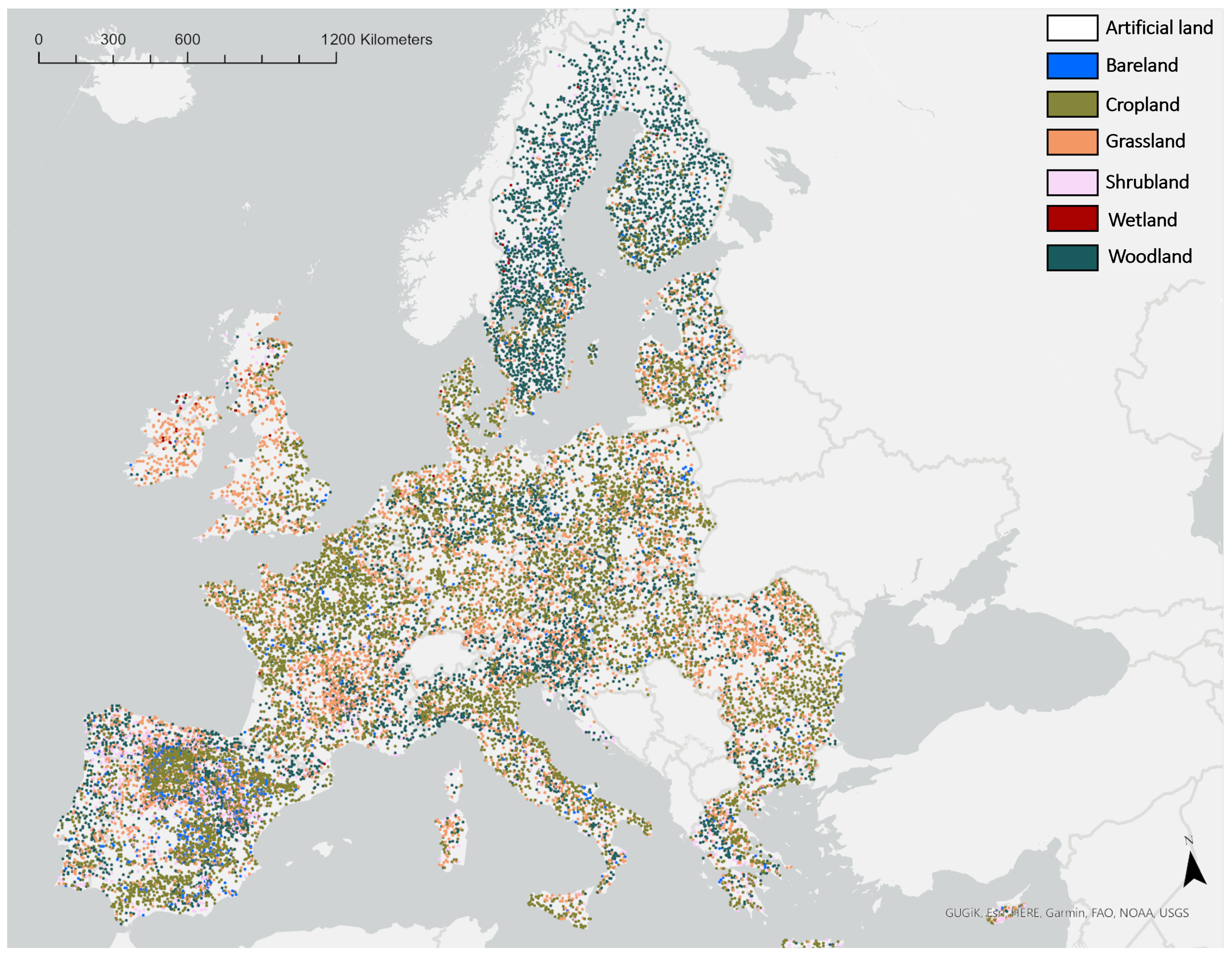
3.1.1. Ground Reference Samples
3.1.2. Input Features
Climate Data
Landsat-8 Bands
Vegetation and Mineral Indices
Topography
3.2. Experiments
3.2.1. Implemented Methods
Bootstrapping Random Forest
Conformalized Quantile Random Forest
Quantile Neural Networks
Quantile Gradient Boosting
Quantile Linear Regression
3.2.2. Evaluation Metrics
Uncertainty
- 1
- Negative Log-Likelihood (NLL): NLL measures the agreement between predicted () and observed values () under the assumption of a Gaussian distribution with a mean of zero and a standard deviation (). The NLL is defined as:
- 2
- Interval Score (IS): The scoring function is designed to evaluate the performance of a predictive model’s interval predictions. It considers the average width of prediction intervals and introduces penalties for observations falling outside the predicted intervals. The parameter and play roles in determining the weighting and conditions for the penalties.The first term of Equation (9) represents the average width of prediction intervals for n number of samples. The second term introduces a penalty for observations, , that fall below the lower bound, , of the prediction interval. The penalty is proportional to the difference between the lower bound and the actual observation. The factor, , scales the penalty, and is the indicator function, which equals 1 if the condition inside is true and 0 otherwise. Similar to the second term, the third term penalizes observations that exceed the upper bound, , of the prediction interval.
- 3
- Prediction Interval Coverage Probability (PICP): The PICP is a fundamental metric used to assess the reliability and calibration of prediction intervals. It quantifies the proportion of observed data points that fall within the model’s prediction intervals. In simpler terms, it shows the coverage of samples. A well-calibrated model would ideally have a PICP close to the specified confidence level, indicating that a given percentage of prediction intervals should encompass the true values. The PICP is calculated as follows:Like Equation (9), U and L are the upper and lower bounds of the prediction intervals and n is the number of samples. A high PICP indicates that a significant portion of the observed data falls within the predicted intervals, reflecting well-calibrated and reliable predictions. Conversely, a low PICP suggests that the prediction intervals may be too narrow, indicating a potential lack of calibration in the model’s uncertainty estimates.
- 4
- Prediction Interval Normalized Average Width (PINAW): The PINAW measures the normalized average width of the prediction intervals relative to the spread of the true values. It provides an indication of how well the width of the prediction intervals corresponds to the variability in the observed data. A lower PINAW indicates that the prediction intervals are narrower compared to the variability of the data.
Accuracy Assessment
- 1
- Root Mean Square Error (RMSE): RMSE is widely used in statistics and data analysis for the accuracy assessment of a model. An accurate model can be assessed by calculating the square root of the mean of the squared differences, which quantifies the average magnitude of prediction errors.
- 2
- Mean Absolute Error (MAE): MAE measures how well predictions or estimates match observed values. MAE calculates the difference between predicted or estimated values and observed values by taking the average of absolute differences instead of squared differences, as does RMSE.
- 3
- Ratio of Performance to Interquartile distance (RPIQ): This metric represents the spread of the population and is calculated using the following equation [64]:The values and represent the 25th and 75th percentiles of the observed samples, respectively, defining the interquartile distance.
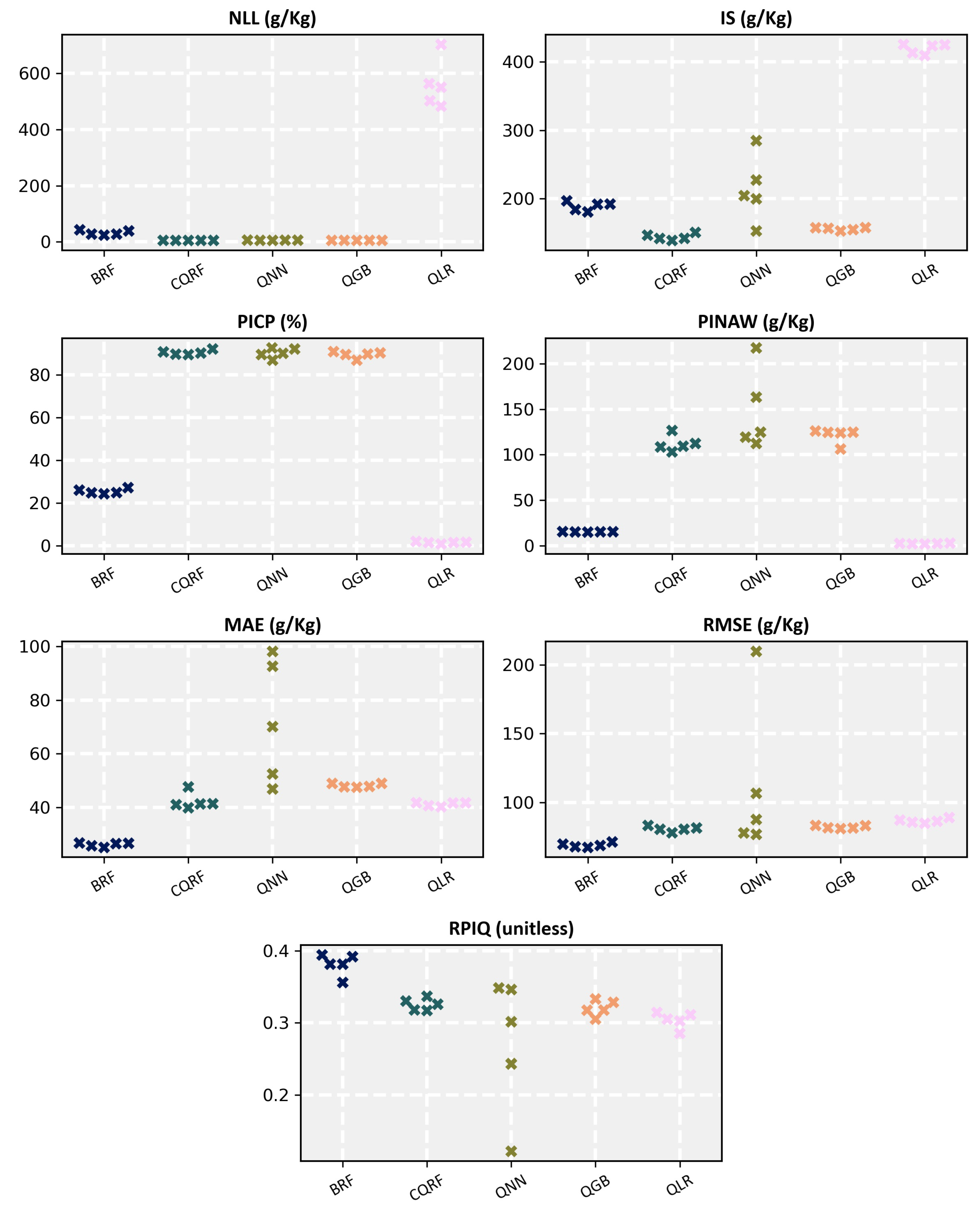
4. Results
4.1. Coverage and Prediction Interval Width: PICP and PINAW
4.2. Accuracy Metrics: RMSE, MAE, and RPIQ
4.3. Scoring Rules: NLL and IS
4.4. Summary of All: Final Score
4.5. Variances of Metric Estimation
5. Discussion
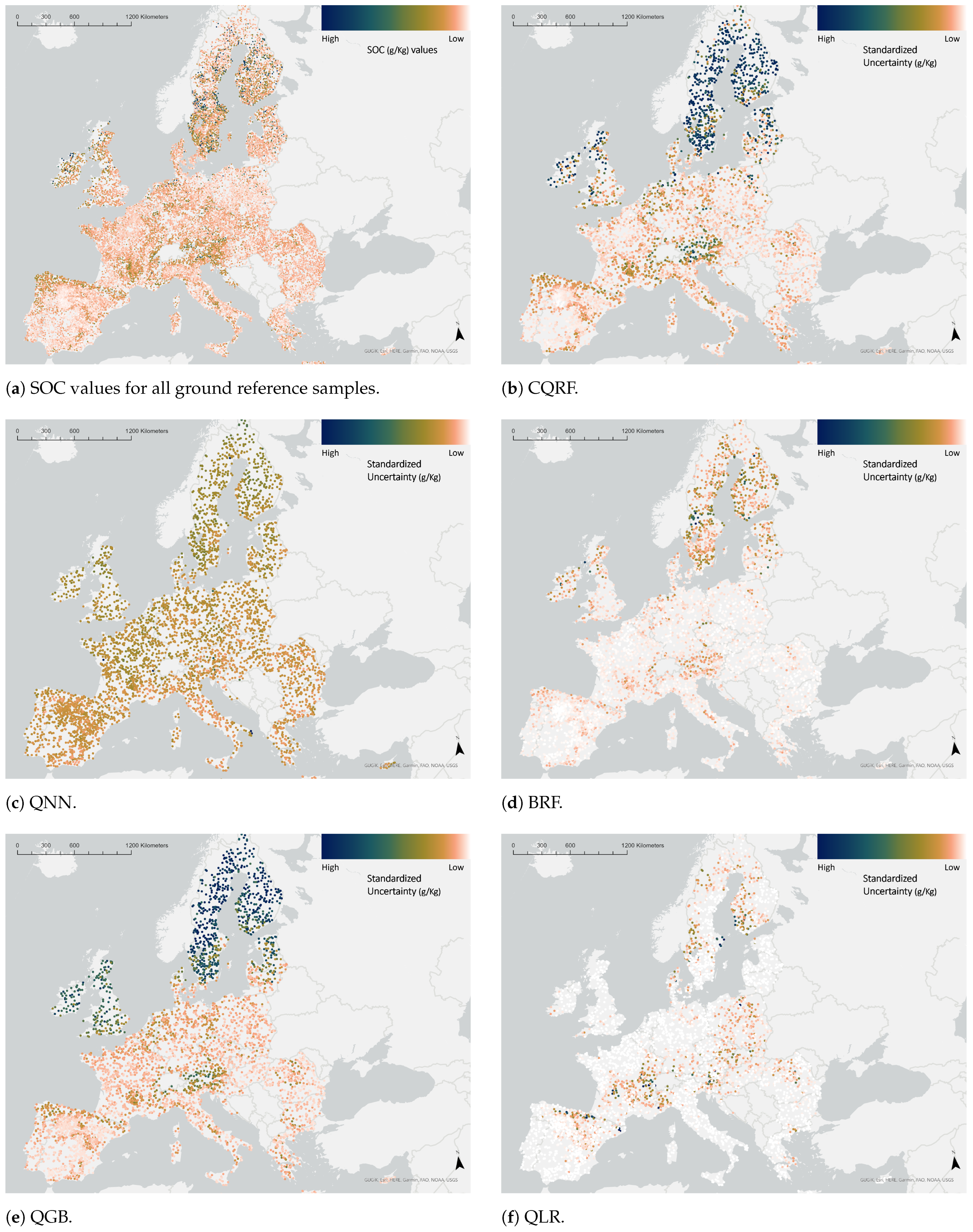
5.1. Understanding Uncertainty in Environmental Contexts
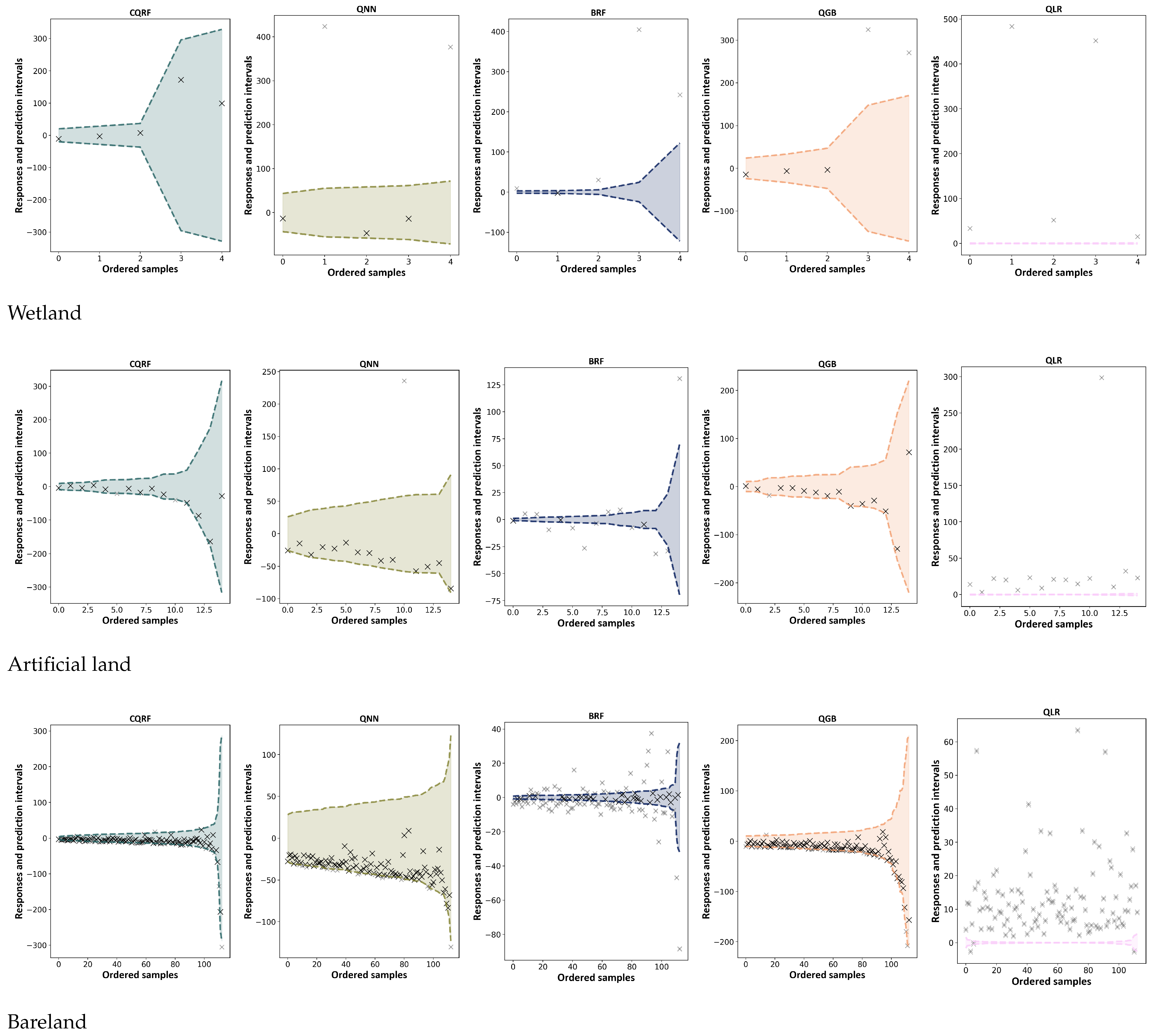
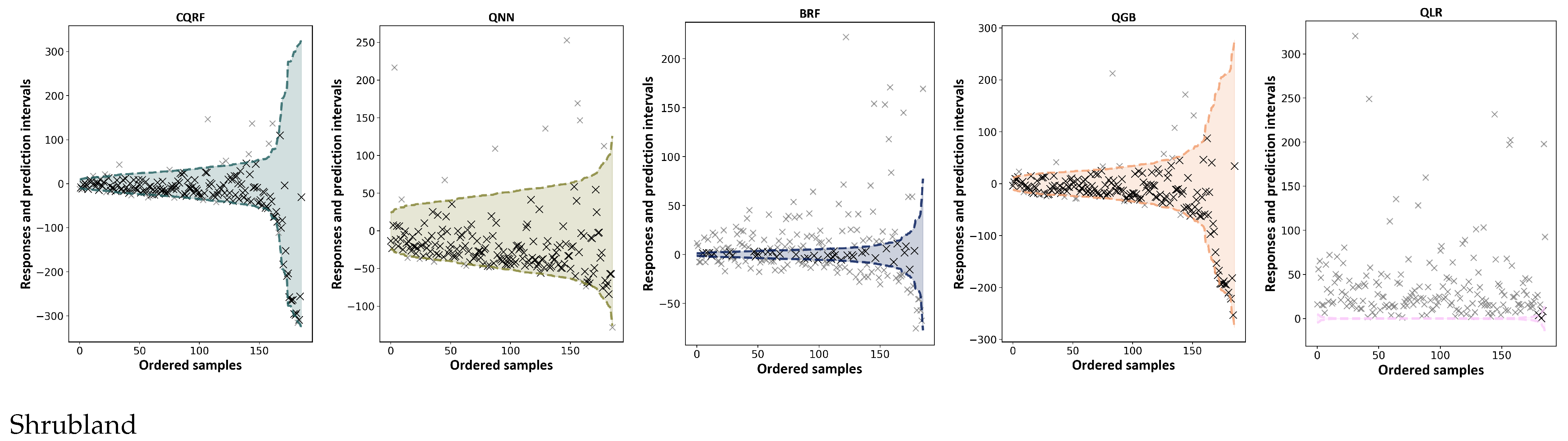
5.2. Empirical Coverage for Low-Sample Classes
6. Conclusions
- Conformal prediction uniquely demonstrates the ability to effectively adjust prediction intervals derived from an ML regression model. This adaptability ensures the generation of uncertainties that closely align with both empirical observations and expert knowledge derived from the natural processes influencing SOC estimation.
- We empirically demonstrated the coverage efficacy of conformal prediction, even for land cover classes characterized by a limited number of samples. This aspect underscores its versatility and reliability across diverse data scenarios.
- In contrast to inherently time-consuming uncertainty quantification techniques, such as bootstrapping, conformal prediction emerges as an efficient solution. Moreover, its versatility extends beyond being a model-specific approach and can be applied to any ML model.
- Beyond its advantages in uncertainty quantification, conformal prediction demonstrates competitive accuracy metrics, as evidenced by lower RMSE and MAE values compared to other methods. This dual proficiency in uncertainty quantification and accuracy sets it apart from other methodologies.
- The uncertainty maps generated by combining conformal prediction with quantile random forest offer a visually captivating representation of the underlying SOC structure. These patterns align seamlessly with our understanding of SOC formation, providing valuable insights into the intricate dynamics of SOC.
Author Contributions
Funding
Data Availability Statement
Conflicts of Interest
References
- Jobbágy, E.G.; Jackson, R.B. The vertical distribution of soil organic carbon and its relation to climate and vegetation. Ecol. Appl. 2000, 10, 423–436. [Google Scholar] [CrossRef]
- Minasny, B.; Malone, B.P.; McBratney, A.B.; Angers, D.A.; Arrouays, D.; Chambers, A.; Chaplot, V.; Chen, Z.S.; Cheng, K.; Das, B.S.; et al. Soil carbon 4 per mille. Geoderma 2017, 292, 59–86. [Google Scholar] [CrossRef]
- Beillouin, D.; Corbeels, M.; Demenois, J.; Berre, D.; Boyer, A.; Fallot, A.; Feder, F.; Cardinael, R. A global meta-analysis of soil organic carbon in the Anthropocene. Nat. Commun. 2023, 14, 3700. [Google Scholar] [CrossRef]
- Rillig, M.C.; van der Heijden, M.G.; Berdugo, M.; Liu, Y.R.; Riedo, J.; Sanz-Lazaro, C.; Moreno-Jiménez, E.; Romero, F.; Tedersoo, L.; Delgado-Baquerizo, M. Increasing the number of stressors reduces soil ecosystem services worldwide. Nat. Clim. Chang. 2023, 13, 478–483. [Google Scholar] [CrossRef] [PubMed]
- Delgado-Baquerizo, M.; Reich, P.B.; Trivedi, C.; Eldridge, D.J.; Abades, S.; Alfaro, F.D.; Bastida, F.; Berhe, A.A.; Cutler, N.A.; Gallardo, A.; et al. Multiple elements of soil biodiversity drive ecosystem functions across biomes. Nat. Ecol. Evol. 2020, 4, 210–220. [Google Scholar] [CrossRef] [PubMed]
- Orr, J.A.; Vinebrooke, R.D.; Jackson, M.C.; Kroeker, K.J.; Kordas, R.L.; Mantyka-Pringle, C.; Van den Brink, P.J.; De Laender, F.; Stoks, R.; Holmstrup, M.; et al. Towards a unified study of multiple stressors: Divisions and common goals across research disciplines. Proc. R. Soc. B 2020, 287, 20200421. [Google Scholar] [CrossRef] [PubMed]
- Powlson, D.; Bhogal, A.; Chambers, B.; Coleman, K.; Macdonald, A.; Goulding, K.; Whitmore, A. The potential to increase soil carbon stocks through reduced tillage or organic material additions in England and Wales: A case study. Agric. Ecosyst. Environ. 2012, 146, 23–33. [Google Scholar] [CrossRef]
- Lin, Y.; Prentice, S.E., III; Tran, T.; Bingham, N.L.; King, J.Y.; Chadwick, O.A. Modeling deep soil properties on California grassland hillslopes using LiDAR digital elevation models. Geoderma Reg. 2016, 7, 67–75. [Google Scholar] [CrossRef]
- Hong, Y.; Munnaf, M.A.; Guerrero, A.; Chen, S.; Liu, Y.; Shi, Z.; Mouazen, A.M. Fusion of visible-to-near-infrared and mid-infrared spectroscopy to estimate soil organic carbon. Soil Tillage Res. 2022, 217, 105284. [Google Scholar] [CrossRef]
- Atwell, M.A.; Wuddivira, M.N. Soil organic carbon characterization in a tropical ecosystem under different land uses using proximal soil sensing technique. Arch. Agron. Soil Sci. 2022, 68, 297–310. [Google Scholar] [CrossRef]
- Taghizadeh-Mehrjardi, R.; Schmidt, K.; Amirian-Chakan, A.; Rentschler, T.; Zeraatpisheh, M.; Sarmadian, F.; Valavi, R.; Davatgar, N.; Behrens, T.; Scholten, T. Improving the spatial prediction of soil organic carbon content in two contrasting climatic regions by stacking machine learning models and rescanning covariate space. Remote Sens. 2020, 12, 1095. [Google Scholar] [CrossRef]
- McBratney, A.B.; Santos, M.M.; Minasny, B. On digital soil mapping. Geoderma 2003, 117, 3–52. [Google Scholar] [CrossRef]
- Behrens, T.; Schmidt, K.; Ramirez-Lopez, L.; Gallant, J.; Zhu, A.X.; Scholten, T. Hyper-scale digital soil mapping and soil formation analysis. Geoderma 2014, 213, 578–588. [Google Scholar] [CrossRef]
- Stumpf, F.; Schmidt, K.; Goebes, P.; Behrens, T.; Schönbrodt-Stitt, S.; Wadoux, A.; Xiang, W.; Scholten, T. Uncertainty-guided sampling to improve digital soil maps. Catena 2017, 153, 30–38. [Google Scholar] [CrossRef]
- Takoutsing, B.; Heuvelink, G.B.; Stoorvogel, J.J.; Shepherd, K.D.; Aynekulu, E. Accounting for analytical and proximal soil sensing errors in digital soil mapping. Eur. J. Soil Sci. 2022, 73, e13226. [Google Scholar] [CrossRef]
- van der Westhuizen, S.; Heuvelink, G.B.; Hofmeyr, D.P.; Poggio, L. Measurement error-filtered machine learning in digital soil mapping. Spat. Stat. 2022, 47, 100572. [Google Scholar] [CrossRef]
- Nelson, M.; Bishop, T.; Triantafilis, J.; Odeh, I. An error budget for different sources of error in digital soil mapping. Eur. J. Soil Sci. 2011, 62, 417–430. [Google Scholar] [CrossRef]
- Heuvelink, G.B. Uncertainty and uncertainty propagation in soil mapping and modelling. In Pedometrics; Springer: Cham, Switzerland, 2018; pp. 439–461. [Google Scholar]
- Schmidinger, J.; Heuvelink, G.B. Validation of uncertainty predictions in digital soil mapping. Geoderma 2023, 437, 116585. [Google Scholar] [CrossRef]
- Goovaerts, P. Geostatistical modelling of uncertainty in soil science. Geoderma 2001, 103, 3–26. [Google Scholar] [CrossRef]
- Webster, R.; Oliver, M.A. Geostatistics for Environmental Scientists; John Wiley & Sons: Hoboken, NJ, USA, 2007. [Google Scholar]
- Malone, B.; McBratney, A.; Minasny, B. Empirical estimates of uncertainty for mapping continuous depth functions of soil attributes. Geoderma 2011, 160, 614–626. [Google Scholar] [CrossRef]
- Fouedjio, F.; Klump, J. Exploring prediction uncertainty of spatial data in geostatistical and machine learning approaches. Environ. Earth Sci. 2019, 78, 38. [Google Scholar] [CrossRef]
- Padarian, J.; Minasny, B.; McBratney, A. Chile and the Chilean soil grid: A contribution to GlobalSoilMap. Geoderma Reg. 2017, 9, 17–28. [Google Scholar] [CrossRef]
- Valle, D.; Izbicki, R.; Leite, R.V. Quantifying uncertainty in land-use land-cover classification using conformal statistics. Remote Sens. Environ. 2023, 295, 113682. [Google Scholar] [CrossRef]
- Kasraei, B.; Heung, B.; Saurette, D.D.; Schmidt, M.G.; Bulmer, C.E.; Bethel, W. Quantile regression as a generic approach for estimating uncertainty of digital soil maps produced from machine-learning. Environ. Model. Softw. 2021, 144, 105139. [Google Scholar] [CrossRef]
- Lagacherie, P.; Arrouays, D.; Bourennane, H.; Gomez, C.; Martin, M.; Saby, N.P. How far can the uncertainty on a Digital Soil Map be known?: A numerical experiment using pseudo values of clay content obtained from Vis-SWIR hyperspectral imagery. Geoderma 2019, 337, 1320–1328. [Google Scholar] [CrossRef]
- Vaysse, K.; Lagacherie, P. Using quantile regression forest to estimate uncertainty of digital soil mapping products. Geoderma 2017, 291, 55–64. [Google Scholar] [CrossRef]
- Meinshausen, N.; Ridgeway, G. Quantile regression forests. J. Mach. Learn. Res. 2006, 7, 983–999. [Google Scholar]
- Cannon, A.J. Quantile regression neural networks: Implementation in R and application to precipitation downscaling. Comput. Geosci. 2011, 37, 1277–1284. [Google Scholar] [CrossRef]
- Minasny, B.; Vrugt, J.A.; McBratney, A.B. Confronting uncertainty in model-based geostatistics using Markov Chain Monte Carlo simulation. Geoderma 2011, 163, 150–162. [Google Scholar] [CrossRef]
- Karunaratne, S.; Bishop, T.; Baldock, J.; Odeh, I. Catchment scale mapping of measureable soil organic carbon fractions. Geoderma 2014, 219, 14–23. [Google Scholar] [CrossRef]
- Solomatine, D.P.; Shrestha, D.L. A novel method to estimate model uncertainty using machine learning techniques. Water Resour. Res. 2009, 45, W00B11. [Google Scholar] [CrossRef]
- Condran, S.; Bewong, M.; Islam, M.Z.; Maphosa, L.; Zheng, L. Machine learning in precision agriculture: A survey on trends, applications and evaluations over two decades. IEEE Access 2022, 10, 73786–73803. [Google Scholar] [CrossRef]
- Saia, S.M.; Nelson, N.G.; Huseth, A.S.; Grieger, K.; Reich, B.J. Transitioning machine learning from theory to practice in natural resources management. Ecol. Model. 2020, 435, 109257. [Google Scholar]
- Xu, F.; Uszkoreit, H.; Du, Y.; Fan, W.; Zhao, D.; Zhu, J. Explainable AI: A brief survey on history, research areas, approaches and challenges. In Proceedings of the Natural Language Processing and Chinese Computing: 8th CCF International Conference, NLPCC 2019, Part II 8, Dunhuang, China, 9–14 October 2019; pp. 563–574. [Google Scholar]
- You, K.; Long, M.; Cao, Z.; Wang, J.; Jordan, M.I. Universal domain adaptation. In Proceedings of the IEEE/CVF Conference on Computer Vision and Pattern Recognition, Long Beach, CA, USA, 15–20 June 2019; pp. 2720–2729. [Google Scholar]
- Raghunathan, A.; Xie, S.M.; Yang, F.; Duchi, J.; Liang, P. Understanding and mitigating the tradeoff between robustness and accuracy. arXiv 2020, arXiv:2002.10716. [Google Scholar]
- Hüllermeier, E.; Waegeman, W. Aleatoric and epistemic uncertainty in machine learning: An introduction to concepts and methods. Mach. Learn. 2021, 110, 457–506. [Google Scholar] [CrossRef]
- Farag, M.; Kierdorf, J.; Roscher, R. Inductive Conformal Prediction for Harvest-Readiness Classification of Cauliflower Plants: A Comparative Study of Uncertainty Quantification Methods. In Proceedings of the IEEE/CVF International Conference on Computer Vision, Paris, France, 2–6 October 2023; pp. 651–659. [Google Scholar]
- Melki, P.; Bombrun, L.; Diallo, B.; Dias, J.; Da Costa, J.P. Group-Conditional Conformal Prediction via Quantile Regression Calibration for Crop and Weed Classification. In Proceedings of the IEEE/CVF International Conference on Computer Vision, Paris, France, 2–6 October 2023; pp. 614–623. [Google Scholar]
- Jensen, V.; Bianchi, F.M.; Anfinsen, S.N. Ensemble conformalized quantile regression for probabilistic time series forecasting. IEEE Trans. Neural Netw. Learn. Syst. 2022. [Google Scholar] [CrossRef]
- Shafer, G.; Vovk, V. A Tutorial on Conformal Prediction. J. Mach. Learn. Res. 2008, 9, 371–421. [Google Scholar]
- Vovk, V.; Gammerman, A.; Shafer, G. Algorithmic Learning in a Random World; Springer: New York, NY, USA, 2005; Volume 29. [Google Scholar]
- Balasubramanian, V.; Ho, S.S.; Vovk, V. Conformal Prediction for Reliable Machine Learning: Theory, Adaptations and Applications; Morgan Kaufmann: Waltham, MA, USA, 2014. [Google Scholar]
- Romano, Y.; Patterson, E.; Candes, E. Conformalized quantile regression. In Proceedings of the 33rd Conference on Neural Information Processing Systems (NeurIPS 2019), Vancouver, BC, Canada, 8–14 December 2019; Volume 32. [Google Scholar]
- Sesia, M.; Candès, E.J. A comparison of some conformal quantile regression methods. Stat 2020, 9, e261. [Google Scholar] [CrossRef]
- Takeuchi, I.; Le, Q.; Sears, T.; Smola, A. Nonparametric quantile estimation. J. Mach. Learn. Res. 2006, 7, 1231–1264. [Google Scholar]
- Koenker, R.; Hallock, K.F. Quantile regression. J. Econ. Perspect. 2001, 15, 143–156. [Google Scholar] [CrossRef]
- Angelopoulos, A.N.; Bates, S. A gentle introduction to conformal prediction and distribution-free uncertainty quantification. arXiv 2021, arXiv:2107.07511. [Google Scholar]
- Abatzoglou, J.T.; Dobrowski, S.Z.; Parks, S.A.; Hegewisch, K.C. TerraClimate, a high-resolution global dataset of monthly climate and climatic water balance from 1958–2015. Sci. Data 2018, 5, 170191. [Google Scholar] [CrossRef] [PubMed]
- Hijmans, R.J.; Cameron, S.E.; Parra, J.L.; Jones, P.G.; Jarvis, A. Very high resolution interpolated climate surfaces for global land areas. Int. J. Climatol. A J. R. Meteorol. Soc. 2005, 25, 1965–1978. [Google Scholar] [CrossRef]
- Sakhaee, A.; Gebauer, A.; Ließ, M.; Don, A. Spatial prediction of organic carbon in German agricultural topsoil using machine learning algorithms. Soil 2022, 8, 587–604. [Google Scholar] [CrossRef]
- Tamburini, G.; Bommarco, R.; Wanger, T.C.; Kremen, C.; Van Der Heijden, M.G.; Liebman, M.; Hallin, S. Agricultural diversification promotes multiple ecosystem services without compromising yield. Sci. Adv. 2020, 6, eaba1715. [Google Scholar] [CrossRef]
- Yang, Q.; Liu, G.; Giannetti, B.F.; Agostinho, F.; Almeida, C.M.; Casazza, M. Emergy-based ecosystem services valuation and classification management applied to China’s grasslands. Ecosyst. Serv. 2020, 42, 101073. [Google Scholar] [CrossRef]
- Alasta, A.F. Using Remote Sensing data to identify iron deposits in central western Libya. In Proceedings of the International Conference on Emerging Trends in Computer and Image Processing, Bangkok, Thailand, 23–24 December 2011; pp. 56–61. [Google Scholar]
- Segal, D. Theoretical basis for differentiation of ferric-iron bearing minerals, using Landsat MSS data. In Proceedings of the Symposium for Remote Sensing of Environment, 2nd Thematic Conference on Remote Sensing for Exploratory Geology, Fort Worth, TX, USA, 6–10 December 1982; pp. 949–951. [Google Scholar]
- Baumann, F.; He, J.S.; Schmidt, K.; Kuehn, P.; Scholten, T. Pedogenesis, permafrost, and soil moisture as controlling factors for soil nitrogen and carbon contents across the Tibetan Plateau. Glob. Chang. Biol. 2009, 15, 3001–3017. [Google Scholar] [CrossRef]
- Don, A.; Schumacher, J.; Scherer-Lorenzen, M.; Scholten, T.; Schulze, E.D. Spatial and vertical variation of soil carbon at two grassland sites—implications for measuring soil carbon stocks. Geoderma 2007, 141, 272–282. [Google Scholar] [CrossRef]
- Carter, B.J.; Ciolkosz, E.J. Slope gradient and aspect effects on soils developed from sandstone in Pennsylvania. Geoderma 1991, 49, 199–213. [Google Scholar] [CrossRef]
- Kakhani, N.; Rangzan, M.; Jamali, A.; Attarchi, S.; Alavipanah, S.K.; Scholten, T. SoilNet: An Attention-based Spatio-temporal Deep Learning Framework for Soil Organic Carbon Prediction with Digital Soil Mapping in Europe. arXiv 2023, arXiv:2308.03586. [Google Scholar]
- Reichstein, M.; Camps-Valls, G.; Stevens, B.; Jung, M.; Denzler, J.; Carvalhais, N.; Prabhat, F. Deep learning and process understanding for data-driven Earth system science. Nature 2019, 566, 195–204. [Google Scholar] [CrossRef] [PubMed]
- Chung, Y.; Char, I.; Guo, H.; Schneider, J.; Neiswanger, W. Uncertainty toolbox: An open-source library for assessing, visualizing, and improving uncertainty quantification. arXiv 2021, arXiv:2109.10254. [Google Scholar]
- Bellon-Maurel, V.; Fernandez-Ahumada, E.; Palagos, B.; Roger, J.M.; McBratney, A. Critical review of chemometric indicators commonly used for assessing the quality of the prediction of soil attributes by NIR spectroscopy. TrAC Trends Anal. Chem. 2010, 29, 1073–1081. [Google Scholar] [CrossRef]
- Feeney, C.; Cosby, B.; Robinson, D.; Thomas, A.; Emmett, B.; Henrys, P. Multiple soil map comparison highlights challenges for predicting topsoil organic carbon concentration at national scale. Sci. Rep. 2022, 12, 1379. [Google Scholar] [CrossRef] [PubMed]
- de Brogniez, D.; Ballabio, C.; Stevens, A.; Jones, R.; Montanarella, L.; van Wesemael, B. A map of the topsoil organic carbon content of Europe generated by a generalized additive model. Eur. J. Soil Sci. 2015, 66, 121–134. [Google Scholar] [CrossRef]
- Hoffmann, U.; Hoffmann, T.; Johnson, E.; Kuhn, N.J. Assessment of variability and uncertainty of soil organic carbon in a mountainous boreal forest (Canadian Rocky Mountains, Alberta). Catena 2014, 113, 107–121. [Google Scholar] [CrossRef]
- Baird, A.J.; Comas, X.; Slater, L.D.; Belyea, L.R.; Reeve, A. Understanding carbon cycling in Northern peatlands: Recent developments and future prospects. Carbon Cycl. North. Peatlands 2009, 184, 1–3. [Google Scholar]
- Barreto, C.; Lindo, Z. Decomposition in peatlands: Who are the players and what affects them? Front. Young Minds 2022, 8, 107. [Google Scholar] [CrossRef]
- Gries, P.; Schmidt, K.; Scholten, T.; Kühn, P. Regional and local scale variations in soil organic carbon stocks in West Greenland. J. Plant Nutr. Soil Sci. 2020, 183, 292–305. [Google Scholar] [CrossRef]
- Lange, M.; Eisenhauer, N.; Sierra, C.A.; Bessler, H.; Engels, C.; Griffiths, R.I.; Mellado-Vázquez, P.G.; Malik, A.A.; Roy, J.; Scheu, S.; et al. Plant diversity increases soil microbial activity and soil carbon storage. Nat. Commun. 2015, 6, 6707. [Google Scholar] [CrossRef]
- Scholten, T.; Baumann, F.; Schleuss, P.M.; He, J.S. Tibet: Soils, climate, vegetation, and land-use feedbacks on the Tibetan Plateau. In Soil and Climate; CRC Press: Boca Raton, FL, USA, 2019. [Google Scholar]


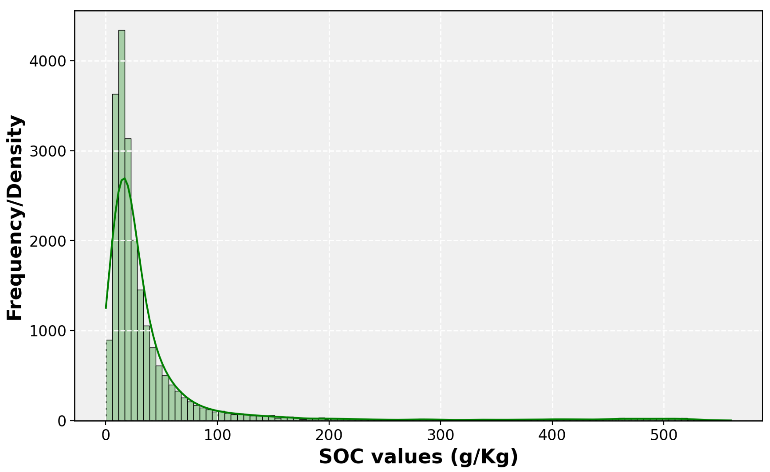
| Mean | s.d. | Min. | Q1 | Median | Q3 | Max. | |
|---|---|---|---|---|---|---|---|
| SOC (g/kg) | 43.27 | 76.70 | 0.1 | 12.5 | 20.4 | 38.6 | 560.2 |
| Category | Number of Features | Spatial Resolution | Temporal Resolution |
|---|---|---|---|
| Climate Data | 12 | ∼4 km | One month |
| Landsat-8 Bands | 7 | 30 m | 16 day |
| Vegetation and Mineral Indices | 5 | 30 m | 16 day |
| Topography | 4 | 30 m | One time mission |
| No | Feature | Description | Unit |
|---|---|---|---|
| 1 | L8B1 | Ultra Blue | |
| 2 | L8B2 | Blue | |
| 3 | L8B3 | Green | |
| 4 | L8B4 | Red | |
| 5 | L8B5 | NIR | |
| 6 | L8B6 | SWIR1 | |
| 7 | L8B7 | SWIR2 | |
| 8 | Clay Minerals | Unitless | |
| 9 | Ferrous Minerals | Unitless | |
| 10 | Carbonate Index | Unitless | |
| 11 | Rock Outcrop Index | Unitless | |
| 12 | NDVI | Unitless | |
| 13 | Elevation | Elevation | m |
| 14 | Slope | Slope | Percent |
| 15 | VBF | Vally bottom flatness | Unitless |
| 16 | TWI | Topography wetness index | Unitless |
| 17 | Actual evapotranspiration | Actual evapotranspiration | mm |
| 18 | pdsi | Palmer Drought Severity Index | Unitless |
| 19 | Climate water deficit | Climate water deficit | mm |
| 20 | Reference evapotranspiration | Reference evapotranspiration | mm |
| 21 | Precipitation accumulation | Precipitation accumulation | mm |
| 22 | Soil moisture | Soil moisture | mm |
| 23 | Surface radiation | Downward surface shortwave radiation | W/m2 |
| 24 | Minimum temperature | Minimum temperature | °C |
| 25 | Maximum temperature | Maximum temperature | °C |
| 26 | Vapor pressure deficit | Vapor pressure deficit | kPa |
| 27 | Vapor pressure | Vapor pressure | kPa |
| 28 | Wind speed | Wind speed at 10 m | m/s |
| Uncertainty | Accuracy | |||||||
|---|---|---|---|---|---|---|---|---|
| Method | NLL | IS | PICP (%) | PINAW | MAE | RMSE | RPIQ | Final Score |
| BRF | 32.06 | 188.89 | 25 | 15.67 | 26.07 | 69.03 | 0.38 | 0.33 |
| CQRF | 4.93 | 143.75 | 90 | 111.91 | 42.20 | 80.79 | 0.33 | 0.31 |
| QNN | 5.89 | 243.99 | 89 | 165.58 | 72.05 | 111.73 | 0.27 | 0.58 |
| QGB | 5.06 | 155.75 | 89 | 124.30 | 48.15 | 82.39 | 0.32 | 0.35 |
| QLR | 550.87 | 419.54 | 2 | 2.24 | 41.145 | 86.59 | 0.30 | 0.64 |
Disclaimer/Publisher’s Note: The statements, opinions and data contained in all publications are solely those of the individual author(s) and contributor(s) and not of MDPI and/or the editor(s). MDPI and/or the editor(s) disclaim responsibility for any injury to people or property resulting from any ideas, methods, instructions or products referred to in the content. |
© 2024 by the authors. Licensee MDPI, Basel, Switzerland. This article is an open access article distributed under the terms and conditions of the Creative Commons Attribution (CC BY) license (https://creativecommons.org/licenses/by/4.0/).
Share and Cite
Kakhani, N.; Alamdar, S.; Kebonye, N.M.; Amani, M.; Scholten, T. Uncertainty Quantification of Soil Organic Carbon Estimation from Remote Sensing Data with Conformal Prediction. Remote Sens. 2024, 16, 438. https://doi.org/10.3390/rs16030438
Kakhani N, Alamdar S, Kebonye NM, Amani M, Scholten T. Uncertainty Quantification of Soil Organic Carbon Estimation from Remote Sensing Data with Conformal Prediction. Remote Sensing. 2024; 16(3):438. https://doi.org/10.3390/rs16030438
Chicago/Turabian StyleKakhani, Nafiseh, Setareh Alamdar, Ndiye Michael Kebonye, Meisam Amani, and Thomas Scholten. 2024. "Uncertainty Quantification of Soil Organic Carbon Estimation from Remote Sensing Data with Conformal Prediction" Remote Sensing 16, no. 3: 438. https://doi.org/10.3390/rs16030438