Enhancing Satellite Image Sequences through Multi-Scale Optical Flow-Intermediate Feature Joint Network

Abstract

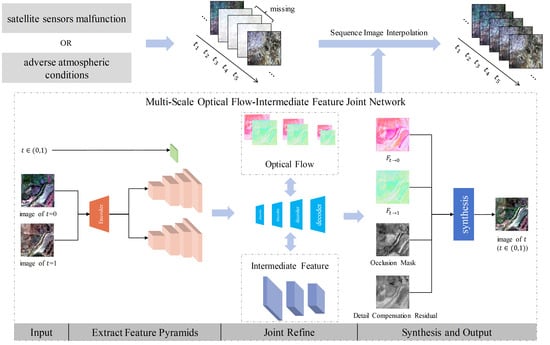
Satellite time-series data contain information in three dimensions—spatial, spectral, and temporal—and are widely used for monitoring, simulating, and evaluating Earth activities. However, some time-phase images in the satellite time series data are missing due to satellite sensor malfunction or adverse atmospheric conditions, which prevents the effective use of the data. Therefore, we need to complement the satellite time series data with sequence image interpolation. Linear interpolation methods and deep learning methods that have been applied to sequence image interpolation lead to large errors between the interpolation results and the real images due to the lack of accurate estimation of pixel positions and the capture of changes in objects. Inspired by video frame interpolation, we combine optical flow estimation and deep learning and propose a method named Multi-Scale Optical Flow-Intermediate Feature Joint Network. This method learns pixel occlusion and detailed compensation information for each channel and jointly refines optical flow and intermediate features at different scales through an end-to-end network together. In addition, we set a spectral loss function to optimize the network’s learning of the spectral features of satellite images. We have created a time-series dataset using Landsat-8 satellite data and Sentinel-2 satellite data and then conducted experiments on this dataset. Through visual and quantitative evaluation of the experimental results, we discovered that the interpolation results of our method retain better spectral and spatial consistency with the real images, and that the results of our method on the test dataset have a 7.54% lower Root Mean Square Error than other approaches.

1. Introduction

Big data in remote sensing refer to the massive volumes of information generated by Earth observation satellites, particularly when dealing with time series data from satellites like MODIS with frequent revisits [1,2]. Remote sensing time series data can be used for monitoring, analyzing, and predicting various natural and human phenomena, including land use/cover change detection, wetland monitoring, crop classification, disaster early warning, etc. [3,4,5,6,7].

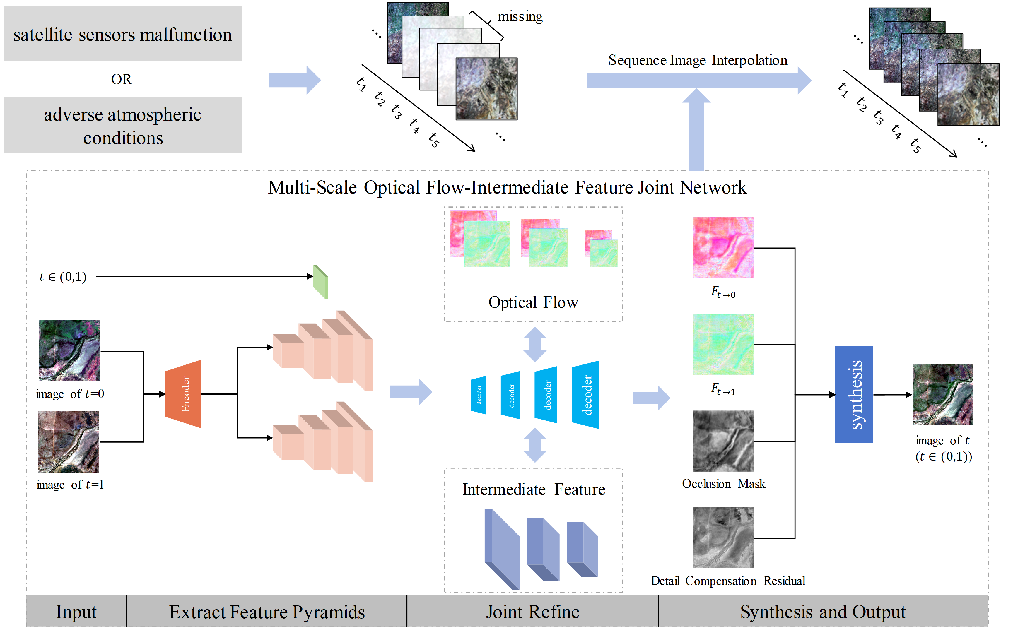
However, satellite sensors may malfunction or there may be adverse atmospheric conditions during the acquisition of remotely sensed data, and these problems often result in missing data for intermediate time phase images, making it impossible to form a complete time series [8,9]. There are three instances of remote sensing data that are missing, shown in Figure 1.

One prevalent approach for filling in the gaps in a sequence of images at intermediate time phases is the use of image interpolation. This technique involves generating the missing images by utilizing information from the images at the preceding and subsequent time phases. Image interpolation is a foundational task in digital image processing and computer vision, classified into intra-image interpolation and inter-image interpolation based on the dimension of interpolation [10]. Inter-image interpolation, also termed sequence image interpolation, focuses on creating multiple new images within a sequence of existing images. Our research involves a comprehensive exploration and generalization of the methodology for sequential image interpolation.

The fundamental approach to sequential image interpolation is pixel-wise linear interpolation. This method employs a linear weighted combination of pixel values at equivalent positions within two adjacent images to compute the pixel values of the intervening image. Vandal et al. [11] compared their deep learning method with linear interpolation and showed that their method is better at time enhancement from 10 min to 1 min for remote sensing data with different spatial resolutions. The requirements for the spectral integrity of interpolated images cannot be met by the simple and consistent weighted linear approach [12].

Shape-based interpolation is a method of interpolating sequential images by extracting the shape contours of an object from an image sequence and interpolating them in accordance with the changes of an object at each time instance. Raya et al. [13] first proposed a shape-based interpolation algorithm, which first segmented the given image data into binary images, then converted the binary images back to gray images, and finally interpolated the gray images. This method is seldom applied to remote sensing data. The reason is that remote sensing data encompass a multitude of objects and intricate textures, which significantly complicates the extraction of contours.

In the last few years, deep learning has achieved a good performance in satellite image processing tasks, including image fusion, image classification, object detection, and picture reconstruction [14,15,16,17,18,19,20,21,22,23]. It employs high-parameter models to comprehend complex textures and spectral features for image interpolation tasks, using the images from two time phases to output the intermediate phase image. Niklaus et al. [24] used a local convolution on two input frames for intermediate frame interpolation. They employed a convolutional neural network (CNN) to learn spatially adaptive filters for each pixel, addressing occlusion, blur, and brightness changes. Jin et al. [25] introduced a separable convolution network for remote sensing sequential image interpolation. This network uses separable 1D convolution kernels to capture spatial features of sequential images. Tests on Landsat-8 and drone data showed its effectiveness in generating high-quality time series interpolation images. For high-resolution images, Peleg et al. [26] proposed an interpolation motion neural network to improve interpolation quality. This network uses a cost-effective structured architecture, end-to-end training, and a multi-scale customized loss function. It classifies interpolation motion estimation, enhancing the interpolation effect and speed on high-resolution images. Deep learning-based interpolation methods show robustness to occlusion, blur, and illumination changes. However, their unpredictability and uninterpretability may introduce noise.

Optical flow is a technique frequently employed in computer vision, primarily for target detection and tracking in satellite image processing [27,28]. It aims to determine the exact location of pixels at each stage within a sequence of images. This technique is instrumental in analyzing the motion and changes of objects across different frames in the sequence.

The accuracy of interpolation can be enhanced by accurately estimating pixel motion and addressing occlusion and blurring when optical flow and deep learning are integrated. This concept is frequently used in the field of video frame interpolation, and effectively increases the precision and speed of interpolation. Liu et al. [29] developed a deep voxel flow layer (DVF), akin to an optical flow field. The method captures the direction of pixel flow between adjacent frames and is trained to generate intermediate frames. Jiang et al. [30] proposed a video interpolation method called Super SloMo, based on a convolutional neural network. It initially calculates the bidirectional optical flow between input frames using a U-Net [31], then linearly combines the bidirectional optical flow according to the time step to obtain the approximate intermediate frame optical flow. This is then refined with another U-Net, while also predicting visibility, distorting and fusing the input frames, and excluding the insignificant. The result of the experiment has shown that the U-Net produces high-quality intermediate frames that surpass those produced by current video frame interpolation techniques in the field of remote sensing. Vandal et al. [11] extended Super SloMo to multiple channels and applied it to the GOES-R/Advanced Baseline Imager mesoscale dataset. This enhances the satellite data with different spatial resolutions from 10 min to 1 min in temporal resolution, enabling more accurate weather detection.

In addition, to enhance the speed and accuracy of frame interpolation, Kong et al. [32] proposed simpler and more efficient model structures. They designed an end-to-end network, IFRNet, which extracts pyramidal features from a given input and subsequently recombines bilateral intermediate streams with robust intermediate features until the desired output is produced. Their progressive intermediate features not only aid in the estimation of intermediate information but also compensate for contextual details, thereby efficiently generating intermediate images. This approach signifies a promising advancement in the field of frame interpolation.

This paper draws inspiration from IFRNet [32], to which we have introduced modifications to tailor it for the task of interpolating sequences of satellite images. As far as we know, this is the first attempt to use the optical flow-based interpolation method on satellite images possessing complex object characteristics. The main work in this article is as follows:

• Given the complexity of objects and the richness of spectra in satellite imagery, we endeavor to integrate optical flow estimation with deep learning. This integration aims to develop a robust method for enhancing satellite image sequences.
• We carried out comprehensive experiments on two time-series satellite datasets—Landsat-8 and Sentinel-2. The results demonstrate that our approach yields lower interpolation errors across the four seasons: spring, summer, autumn, and winter. This evidence substantiates that our method can be effectively applied to the interpolation of satellite image sequences in various seasons.

The remainder of this paper is organized as follows: Section 2 provides a detailed description of the satellite datasets and the proposed methodology. The experiments and their results are presented in Section 3. Section 4 offers an in-depth discussion on the rationale behind the results. Finally, Section 5 draws conclusions from the study.

2. Materials and Methods

2.1. Datasets

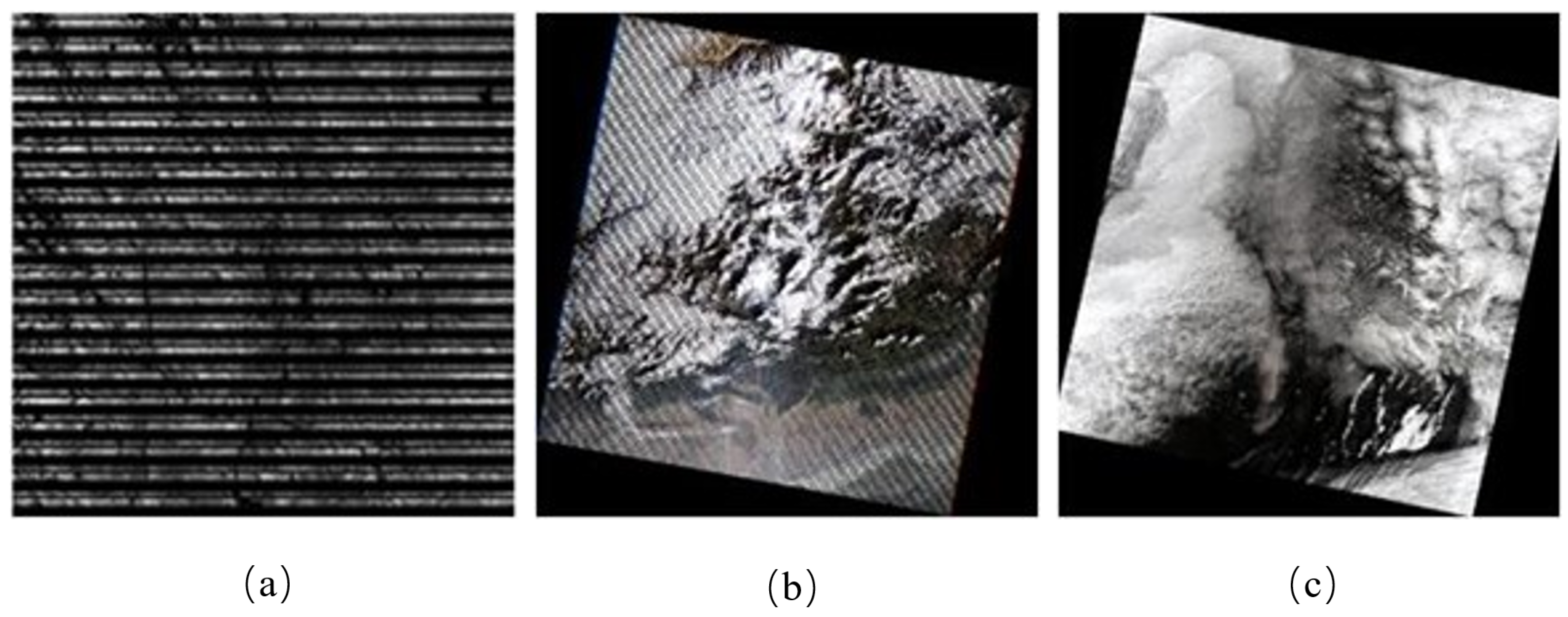
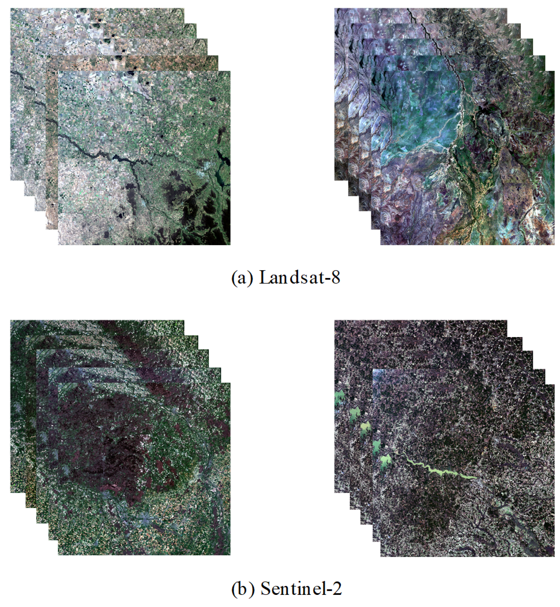
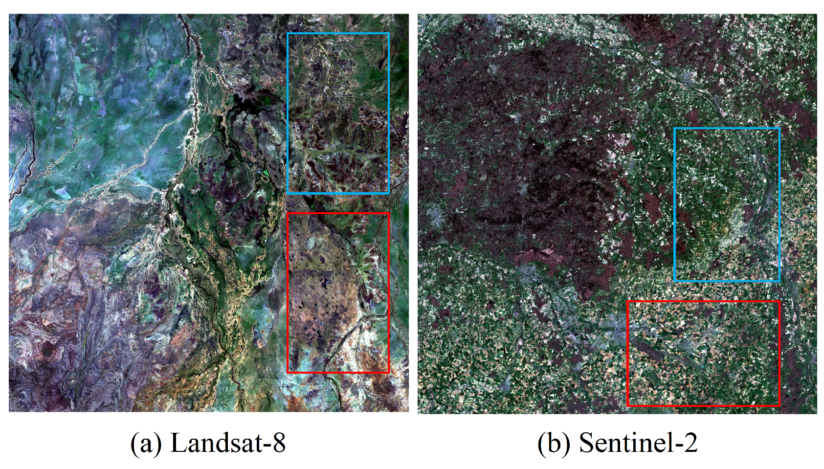
We selected data from two satellites—Landsat-8 and Sentinel-2—consisting of eight and four time series. Their details are given in

Table 1. The details of the Landsat-8 satellite dataset. This table contains the path and row, the acquisition date, the latitude and longitude of the image center point, and the number of phases included for each Landsat-8 satellite time series.

Path,Row	Date	Center Latitude	Center Longitude	Phase Number
91,78	21 June 2022	25°59${}^{\prime }$42${}^{″}$S	150°32${}^{\prime }$35${}^{″}$E	5
	7 July 2022
	23 July 2022
91,79	8 August 2022	27°26${}^{\prime }$2${}^{″}$S	150°11${}^{\prime }$2${}^{″}$E	5
	24 August 2022
91,84	20 January 2019	34°36${}^{\prime }$50${}^{″}$S	148°16${}^{\prime }$34${}^{″}$E	5
	5 February 2019
	21 February 2019
	9 March 2019
	24 March 2019
92,85	20 January 2022	36°2${}^{\prime }$46${}^{″}$S	147°51${}^{\prime }$58${}^{″}$E	5
	5 February 2022
	21 February 2022
	9 March 2022
	24 March 2022
99,73	31 March 2018	18°47${}^{\prime }$24${}^{″}$S	139°53${}^{\prime }$38${}^{″}$E	10
	16 April 2018
	2 May 2018
	18 May 2018
	3 June 2018
99,74	7 September 2018	20°13${}^{\prime }$55${}^{″}$S	139°33${}^{\prime }$40${}^{″}$E	10
	23 September 2018
	9 October 2018
	25 October 2018
	1 November 2018

and 

Table 2. The details of the Sentinel-2 satellite dataset. This table contains the tile ID, the acquisition date, the latitude and longitude of the image center point, and the number of phases included of each Landsat-8 satellite time series.

Tile ID	Date	Center Latitude	Center Longitude	Phase Number
18STF	11 January 2019	36°31${}^{\prime }$12${}^{″}$N	77°44${}^{\prime }$14${}^{″}$W	5
	16 January 2019
	21 January 2019
	26 January 2019
	31 January 2019
31TDN	26 March 2020	47°21${}^{\prime }$29${}^{″}$N	2°24${}^{\prime }$8${}^{″}$E	5
	31 March 2020
	5 April 2020
	10 April 2020
	15 April 2020
30TXT	7 July 2020	47°20${}^{\prime }$28${}^{″}$N	0°56${}^{\prime }$57${}^{″}$W	5
	12 July 2020
	17 July 2020
	22 July 2020
	27 July 2020
35TNM	28 September 2018	46°27${}^{\prime }$26${}^{″}$N	27°42${}^{\prime }$52${}^{″}$E	5
	3 October 2018
	8 October 2018
	23 October 2018
	18 October 2018

, and each time series contains images from five time phases. For the Landsat-8 satellite dataset, we used seven bands: coastal, blue, green, red, near-infrared, short-wave infrared-1, and short-wave infrared-2, all with a spatial resolution of 30 m and a size of 5120 × 5120 per image. Figure 2a shows two examples of time series of the Landsat-8 satellite data. For the Sentinel-2 satellite dataset, we used 8 bands, including blue, green, red, 3 vegetation red edge, near-infrared (wide), and near-infrared (narrow), of which 4 bands, 3 vegetation red edge and near-infrared (narrow), have a spatial resolution of 20 m and a size of 5490 × 5490, and the other bands have a spatial resolution of 10 m and a size of 10,980 × 10,980 per image. The time resolution of the Landsat-8 dataset and the Sentinel-2 dataset is 16 days and 5 days, respectively. Figure 2b shows two examples of time series of the Sentinel-2 satellite data.

In addition, we chose two satellite datasets from latitudes that differ by about ten degrees to ensure climate consistency. The two satellite datasets cover the four seasons: spring, summer, autumn and winter, respectively. The cloud coverage of the images for each temporal phase of both datasets is within 5%.

2.2. Interpolation Model

The objective of satellite image sequencing is to utilize two time-phase images, $I_0$ and $I_1$, to interpolate an image for a specific intermediate time phase t, thereby completing the satellite image sequence. We assume that the two time phases are 0 and 1, and the interpolated result is denoted as ${\widehat{I}}_t$. The interpolation model can be represented as Equation (1):

$${\widehat{I}}_t=f(I_0,I_1,t),$$

(1)

where $t\in [0,1]$ signifies the time interval between the intermediate time phase to be interpolated and time phase 0. $f\left(x\right)$ symbolizes the non-linear relationship between $I_0$, $I_1$, t, and ${\widehat{I}}_t$. In this study, the non-linear relationship $f\left(x\right)$ is approximated using a neural network.

2.3. Architecture of the Model

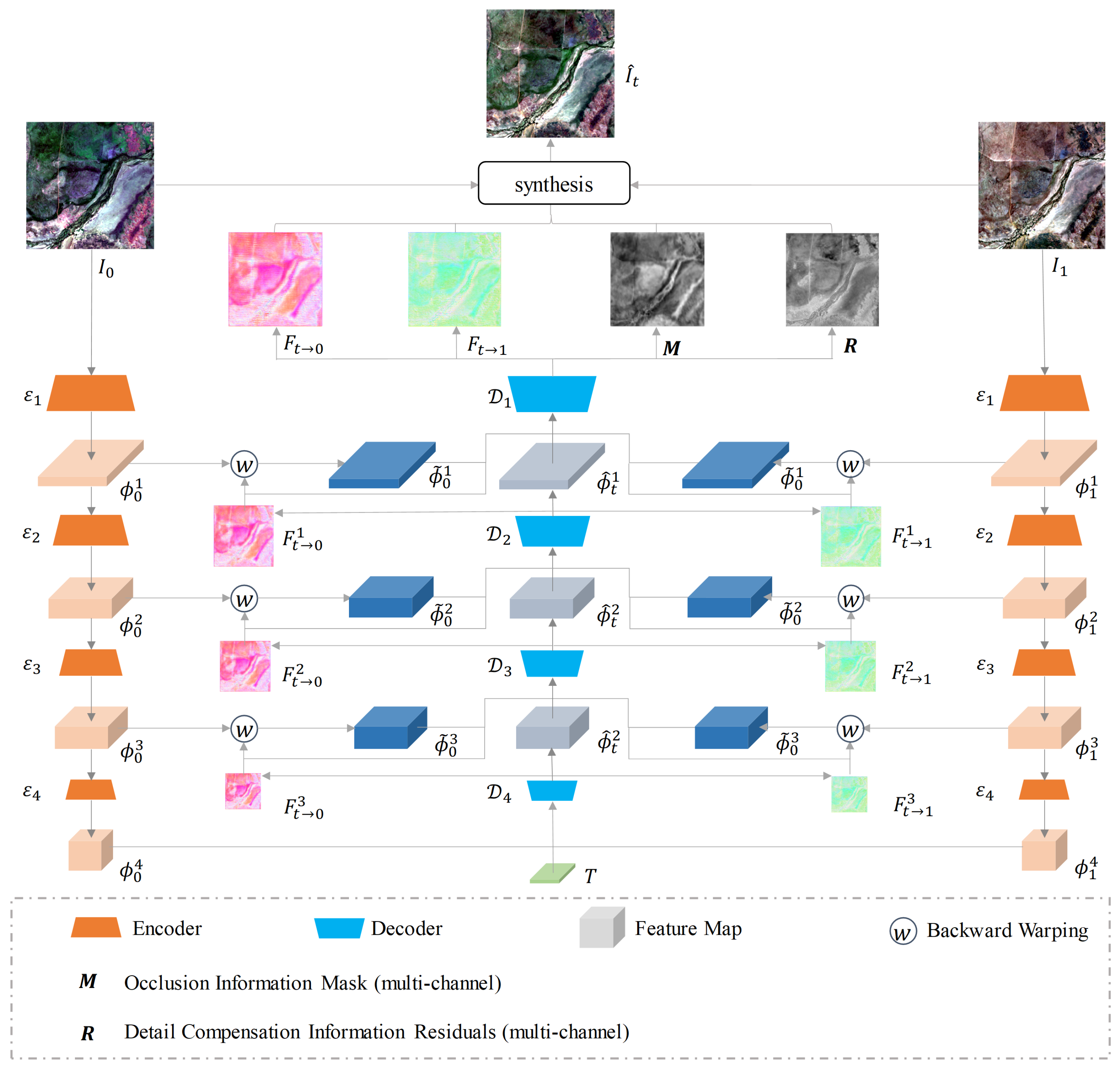
The network architecture in this paper is depicted in Figure 3, and comprises two main components: an encoder and a decoder. The network accepts images from the two time phases ($I_0,I_1$) as well as the intermediate phase T(t) as inputs, which aligns with Equation (1). It generates an image of the intermediate time phase ${\widehat{I}}_t$ by collaboratively and interactively enhancing the images from the two time phases. It learns the intermediate optical flow field and intermediate features across various scales during this process. The following is a detailed explanation of this network.

2.3.1. Extraction of Feature Pyramids

The encoder $\epsilon$ contains four sub-encoders ${\epsilon }^k(k\in \{1,2,3,4\})$. Each sub-encoder has two convolutional layers and one activation layer. The activation function makes use of the PReLU [33]. The input data are two time phase images, $I_0,I_1$, in a satellite image sequence, and the purpose is to extract the feature pyramid ${\varphi }_0$,${\varphi }_1$ containing four scales from the two images. The encoder can be expressed as Equation (2):

$$\epsilon \left([I_0,I_1]\right)=[{\varphi }_0^1,{\varphi }_1^1],[{\varphi }_0^2,{\varphi }_1^2],[{\varphi }_0^3,{\varphi }_1^3],[{\varphi }_0^4,{\varphi }_1^4],$$

(2)

where $I_0$ and $I_1$ are instances of the parameters in Equation (1). ${\varphi }_0^k$,${\varphi }_1^k(k\in \{1,2,3,4\})$ is the four-scale features extracted from $I_0$ and $I_1$.

2.3.2. Joint Refinement of Optical Flow-Intermediate Feature

The decoder $\mathcal{D}$ is composed of four sub-decoders, ${\mathcal{D}}^k(k\in \{1,2,3,4\})$. These sub-decoders iteratively refine the intermediate optical flow by backward warping the pyramidal features ${\varphi }_0^k$ and ${\varphi }_1^k$ through the intermediate optical flow fields $F_{t\to 0}^k$ and $F_{t\to 1}^k$. Each sub-decoder also outputs a higher-level reconstructed intermediate feature ${\widehat{\varphi }}_t^k$, which compensates for the missing image information caused by the backward warping. The subsequent sub-decoder generates an improved intermediate optical flow, $F_{t\to 0}^k$ and $F_{t\to 1}^k$, which can be more accurately pixel-aligned to produce better ${\tilde{\varphi }}_0^k$ and ${\tilde{\varphi }}_1^k$. This, in turn, enhances the reconstruction of intermediate features at higher levels. Therefore, this decoder facilitates the simultaneous enhancement of both the intermediate optical flow and the intermediate features, contributing to a more accurate and detailed interpolation of satellite image sequences. The decoders ${\mathcal{D}}^4$ and ${\mathcal{D}}^1$ are expressed as Equations (3) and (4). The decoders ${\mathcal{D}}^2$ and ${\mathcal{D}}^3$ are expressed as Equation (5):

$$\left[\begin{array}{c}{F}_{t\to 0}^3,F_{t\to 1}^3,{\widehat{\varphi }}_t^3\end{array}\right]={\mathcal{D}}^4\left([{\varphi }_0^4,{\varphi }_1^4,T]\right)$$

(3)

$$[F_{t\to 0},F_{t\to 1},M,R]={\mathcal{D}}^1\left(\left[F_{t\to 0}^1,F_{t\to 1}^1,{\widehat{\varphi }}_t^1,{\tilde{\varphi }}_0^1,{\tilde{\varphi }}_1^1\right]\right)$$

(4)

$$\left[F_{t\to 0}^{k-1},F_{t\to 1}^{k-1},{\widehat{\varphi }}_t^{k-1}\right]={\mathcal{D}}^k\left(\left[F_{t\to 0}^k,F_{t\to 1}^k,{\widehat{\varphi }}_t^k,{\tilde{\varphi }}_0^k,{\tilde{\varphi }}_1^k\right]\right)k\in \{2,3\},$$

(5)

where T represents the single-channel data of size 1 × H × W, which is extended by the intermediate time phase t as defined in Equation (1). The warped images ${\tilde{\varphi }}_0^k$ and ${\tilde{\varphi }}_1^k$ are generated by warping the pyramidal features ${\varphi }_0^k$ and ${\varphi }_1^k$ backward through the intermediate optical flow. This process is governed by Equations (6) and (7):

$${\tilde{\varphi }}_0^k=w({\varphi }_0^k,F_{t\to 0}^k),k\in \{1,2,3\}$$

(6)

$${\tilde{\varphi }}_1^k=w({\varphi }_1^k,F_{t\to 1}^k),k\in \{1,2,3\},$$

(7)

where w means backward warping.

2.3.3. Synthesis of Intermediate Images

The rear stage encoder ${\mathcal{D}}^1$ outputs the intermediate bidirectional optical flow fields $F_{t\to 0}$ and $F_{t\to 1}$, a mask M, and a residual R. All of these outputs are the same size as the input image. The mask M is generated by passing through a sigmoid layer, and its values range from 0 to 1. This mask contains the extracted bidirectional occlusion information. The residual R compensates for details such as the presence of regions in the target image that have been occluded in the images from the preceding and subsequent time phases, as well as the contours of objects. Both the mask M and the residual R have the same number of channels as the input image. In summary, the final synthesis of the image at the intermediate time phase t is given by Equation (8):

$${\widehat{I}}_t=M\odot {\tilde{I}}_0+(1-M)\odot {\tilde{I}}_1+R,$$

(8)

where ${\tilde{I}}_0=w(I_0,F_{t\to 0}),{\tilde{I}}_1=w(I_1,F_{t\to 1})$, ⊙ denotes element-wise multiplication.

2.3.4. Details of the Model

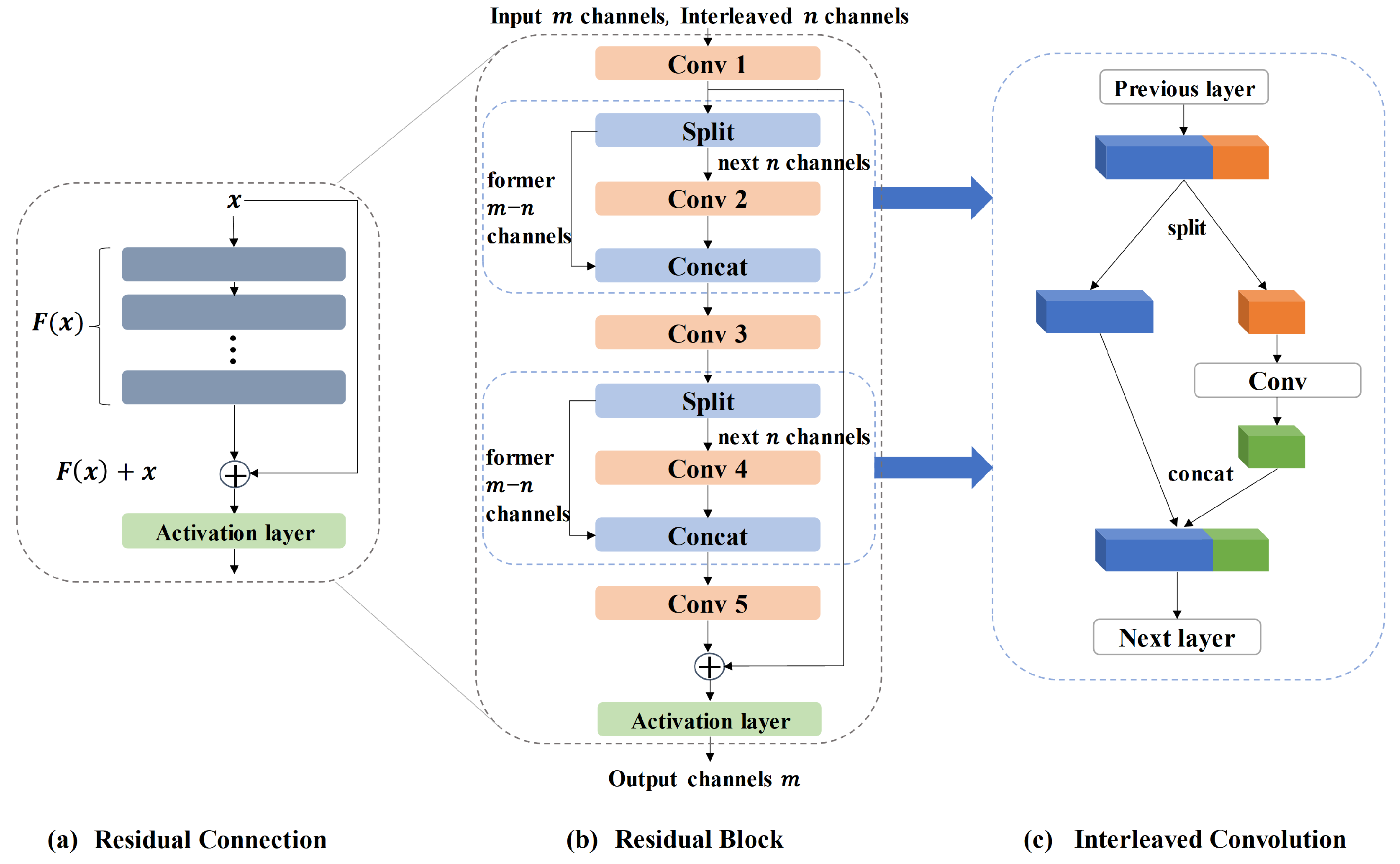
The feature pyramid extracted from the image by the encoder comprises four scales with 32, 48, 72, and 96 channels, respectively. Each sub-decoder in the network contains a convolutional layer, a residual block, and an inverse convolutional layer, all followed by a PReLU activation function.

The structure of the residual block is shown in Figure 4. It includes five convolutional layers. Convolutional layers 2 and 4 update only a subset of the channels of the output feature maps from the previous convolutional layer. These updated outputs are then spliced with the remaining channel feature maps before being input into convolutional layers 3 and 5, respectively. This process is performed in the channel dimension.

The residual block adopts the concept of residual connections [34]. The feature maps output from the convolutional layer 5 are added to the input feature maps of the residual block. The final output of the residual block is obtained through the PReLU activation function. This operation enhances the network’s ability to transmit information, preventing issues such as gradient explosion and gradient disappearance, which could halt information transmission. As a result, the network’s characterization ability is improved, and network degradation is prevented. The residual block also incorporates the concept of interleaved convolution [35]. In this approach, convolutional layers 2 and 4 convolve only some of the channels of the output results of convolutional layers 1 and 3, respectively. The convolved results are then spliced with the channels not involved in this convolution. This operation reduces the number of parameters in the convolution kernel and the amount of computation, thereby enhancing the efficiency and speed of the model.

2.4. Loss Functions

The loss function we use is a linear combination of the reconstruction loss ${\mathcal{L}}_r$, the feature space geometric consistency loss ${\mathcal{L}}_g$, and the spectral loss ${\mathcal{L}}_{sam}$, which is expressed as Equation (9):

$$\mathcal{L}={\lambda }_r{\mathcal{L}}_r+{\lambda }_g{\mathcal{L}}_g+{\lambda }_{sam}{\mathcal{L}}_{sam}.$$

(9)

We set the weight of each loss function as ${\lambda }_r=0.1,{\lambda }_g=0.01,{\lambda }_{sam}=0.5$.

2.4.1. Reconstruction Loss

The reconstruction loss ${\mathcal{L}}_r$ shows the pixel difference between the real image $I_t$ and the interpolated result ${\widehat{I}}_t$; the reconstruction loss formula used in this paper is shown in Equation (10):

$${\mathcal{L}}_r=\rho ({\widehat{I}}_t-I_t)+{\mathcal{L}}_{cen}({\widehat{I}}_t,I_t),$$

(10)

where $\rho \left(x\right)={(x^2+{ϵ}^2)}^{\alpha }$ with $\begin{array}{c}\hfill \alpha =0.5,ϵ={10}^{-3}\end{array}$ is the Charbonnier loss [36], which is a more robust loss function than the Mean Square Error (MSE), avoids the oversensitivity of MSE and can better handle outliers, while ${\mathcal{L}}_{cen}$ is the census loss, which calculates the soft Hamming distance between census-transformed [37] image patches of size 7 × 7.

2.4.2. Feature Space Geometric Consistency Loss

The pyramid features ${\varphi }_0^k,{\varphi }_1^k(k\in \{1,2,3,4\})$, extracted by the encoder $ϵ$, are in a sense equivalent to the intermediate feature ${\widehat{\varphi }}_t^k$ reconstructed by the decoder ${\mathcal{D}}_{k+1}$. Inspired by the local geometric alignment property of the census transform, the present experiments first extract the features ${\varphi }_t^k$ from the real image $I_t$ using the same parameter of the common encoder $\epsilon$. Then, the census loss ${\mathcal{L}}_{cen}$ [38] is extended to the multi-scale feature space for asymptotic supervision, and the soft Hamming distance between the 3 × 3 blocks of feature maps corresponding to the census transform is computed based on the channel dimension. This loss can be expressed as Equation (11):

$${\mathcal{L}}_g=\sum _{k=1}^3{\mathcal{L}}_{cen}({\widehat{\varphi }}_t^k,{\varphi }_t^k).$$

(11)

The pyramidal features extracted by the encoder $ϵ$ contain low-level structural information that is useful for frame synthesis, and the addition of this loss function regularizes the reconstructed intermediate features to maintain a better geometric layout.

2.4.3. Spectral Loss

The spectral loss ${\mathcal{L}}_{sam}$ quantifies the degree of spectral similarity between images by calculating the cosine of the spectral vectors between the interpolated result ${\widehat{I}}_t$ and the real image $I_t$, which is calculated as Equation (12):

$${\mathcal{L}}_{sam}=\frac{1}{NHW}\sum _{n=1}^N\sum _{i=1}^H\sum _{j=1}^W\left|\frac{\langle {\widehat{y}}_{n,i,j},y_{n,i,j}\rangle }{|{\widehat{y}}_{n,i,j}{|}_2{\left|y_{n,i,j}\right|}_2}-1\right|,$$

(12)

where $〈·,·〉$ denotes the inner product, ${\left|·\right|}_2$ is the Euclidean norm, N, H, and W are the number of channels, height, and width of the image, respectively, and ${\widehat{y}}_{n,i,j},y_{n,i,j}$ are the spectral vectors of the interpolated resultant image and the real image at pixel point $(i,j)$, respectively.

3. Experiments and Results

3.1. Experiments Strategy

As shown in

Table 3. Setup of multi-temporal image interpolation experiments. We set up four sets of experiments using the Landsat-8 satellite dataset, and in each set of experiments the inputs are Input Image 1 and Input Image 2, as well as the intermediate time phase t (Input Time Phase). The interpolated results are compared with the Reference Image (the real image).

Experiment ID	Path,Row	Input Image 1	Input Image 2	Reference Image	Input Time Phase
1	91,84	20 January 2019	24 March 2019	5 February 2019	0.25
				21 February 2019	0.5
				9 March 2019	0.75
	92,85	20 January 2022	24 March 2022	5 February 2022	0.25
				21 February 2022	0.5
				9 March 2022	0.75
2	99,73	31 March 2018	3 June 2018	16 April 2018	0.25
				2 May 2018	0.5
				18 May 2018	0.75
	99,74	31 March 2018	3 June 2018	16 April 2018	0.25
				2 May 2018	0.5
				18 May 2018	0.75
3	91,78	21 June 2022	24 August 2022	7 July 2022	0.25
				23 July 2022	0.5
				8 August 2022	0.75
	91,79	21 June 2022	24 August 2022	7 July 2022	0.25
				23 July 2022	0.5
				8 August 2022	0.75
4	99,73	7 September 2018	1 November 2018	23 September 2018	0.25
				9 October 2018	0.5
				25 October 2018	0.75
	99,74	7 September 2018	1 November 2018	23 September 2018	0.25
				9 October 2018	0.5
				25 October 2018	0.75

and 

Table 4. Setup of multi-temporal image interpolation experiments. We set up four sets of experiments using the Sentinel-2 satellite dataset, and in each set of experiments the inputs are Input Image 1 and Input Image 2, as well as the intermediate time phase t (Input Time Phase). The interpolated results are compared with the Reference Image (the real image).

Experiment ID	Tile ID	Input Image 1	Input Image 2	Reference Image	Input Time Phase
1	18STF	11 January 2019	31 January 2019	16 January 2019	0.25
				21 January 2019	0.5
				26 January 2019	0.75
2	31TDN	26 March 2020	15 April 2020	31 March 2020	0.25
				5 April 2020	0.5
				10 April 2020	0.75
3	30TXT	7 July 2020	27 July 2020	12 July 2020	0.25
				17 July 2020	0.5
				22 July 2020	0.75
4	35TNM	28 September 2018	18 October 2018	3 October 2018	0.25
				8 October 2018	0.5
				13 October 2018	0.75

, we set up four sets of experiments for the Landsat-8 and Sentinel-2 satellite datasets, respectively. Each set of experimental data contains two time series for the Landsat-8 satellite, and there is one time series for the Sentinel-2 satellite, and each time series has 5 time-phase images. In each group of experiments, the image of phase 1 and phase 5, the intermediate time phase $t(t\in \{0.25,0.5,0.75\left\}\right)$ and the image of the intermediate time phase t are used as network inputs to train the network and estimate the intermediate images of phase 2, phase 3, and phase 4. The output results are compared with the reference images. The detailed training process is shown in Algorithm 1.

Algorithm 1 Training process.

$//$ For each set of experiments for each $i\in [1,8]$ do     Input Image 1: Image of the first time phase $I_0^i$     Input Image 2: Image of the last time phase $I_1^i$     Input Time Phase: the intermediate time phase $t(t\in \{0.25,0.5,0.75\left\}\right)$     Input Reference Image: Image of the intermediate time phase $I_t^i$     train$(I_0^i,I_1^i,I_t^i)$     weight initialized randomly     ${\widehat{I}}_t^i=f(I_0^i,I_1^i,t)$     ${\mathcal{L}}^i={\lambda }_r{\mathcal{L}}_r^i(I_t^i,{\widehat{I}}_t^i)+{\lambda }_g{\mathcal{L}}_g^i(I_t^i,{\widehat{I}}_t^i)+{\lambda }_{sam}{\mathcal{L}}_{sam}^i(I_t^i,{\widehat{I}}_t^i)$     weight save as $W_i$ end for

Due to the limited computer memory, the images need to be trained in blocks. Each scene image is divided into a collection of blocks with a size of 256 × 256. Among them, there are 400 blocks per image for Landsat-8 data and 1764 blocks per image for Sentinel-2 data. The division strategy of the two satellite datasets is shown in Figure 5. The red box is the validation sample, the blue box is the testing sample, and the others are the training samples. The ratio of the three types of samples is 1:1:8. In addition, in order to make the network training more stable and accelerate convergence, the data need to be preprocessed before entering the network training. The range of Landsat-8 data and Sentinel-2 data used in this experiment is [0, 65,535], so the input data are normalized as follows:

$$x^{\prime }=\frac{x-min\left(x\right)}{max\left(x\right)-min\left(x\right)},$$

(13)

where $min\left(x\right)$ is 0 and $max\left(x\right)$ is 65,535.

In addition, the experiment also sets up a data augmentation strategy: randomly flip horizontally or vertically and randomly reverse the image sequence to improve the robustness and generalization ability of the model. In order to improve network convergence, we train the network using the adaptive moment estimation (Adam) [39] optimization method and a learning rate decay strategy with cosine annealing [40].

This experiment is implemented using Python language coding and uses the PyTorch deep learning library to implement the proposed network model. An NVIDIA GeForce RTX 3060Ti GPU is used for training.

3.2. Evaluation Indicator

We evaluate the experimental results using three metrics: Root Mean Square Error (RMSE) [41], Structural Similarity (SSIM) [42], and Peak Signal-to-Noise Ratio (PSNR) [42].

RMSE reflects the change in pixel error between the interpolated resultant image ${\widehat{I}}_t$ and the true image $I_t$, which is calculated as in Equation (14):

$$RMSE=\sqrt{\frac{1}{W·H}\sum \left({∥{\widehat{I}}_t-I_t∥}_2\right)},$$

(14)

where W and H are the width and height of the image. The range of the $RMSE$ is related to the size of the pixel values of the image, and the smaller the value, the closer the interpolated resultant image is to the real image.

SSIM is based on the visual characteristics of the human eye and measures the similarity between the interpolated image and the reference image in three respects—luminance $L(X,Y)$, contrast $C(X,Y)$, and structure $S(X,Y)$—which is calculated as in Equation (15):

$$SSIM(X,Y)=L(X,Y)·C(X,Y)·S(X,Y),$$

(15)

where $L(X,Y)=\frac{2u_X{u}_Y+C_1}{u_X^2+u_Y^2+C_1}$, $C(X,Y)=\frac{2{\sigma }_X{\sigma }_Y+C_2}{{\sigma }_X^2+{\sigma }_Y^2+C_2}$, $S(X,Y)=\frac{{\sigma }_{XY}+C_3}{{\sigma }_X{\sigma }_Y+C_3}$, ${\mu }_X,{\sigma }_X$ are the mean and standard deviation of the experimental result X; ${\mu }_Y,{\sigma }_Y$ are the mean and standard deviation of the reference image Y, respectively; ${\sigma }_{XY}$ is the correlation coefficient between the experimental result X and the reference image Y. $C_1,C_2,C_3$ are constants to prevent the denominator from becoming zero, usually set as $C_1={(K_1·L)}^2,C_2={(K_2·L)}^2,C_3=\frac{C_2}{2},K_1=0.01,K_2=0.03,L=255$. The value of SSIM ranges from 0 to 1, and the larger the value, the more similar the interpolated image and the reference image are, and vice versa.

PSNR is the ratio between the maximum possible power of a signal and the power of the noise that affects the fidelity of its representation, measured in dB, which is calculated as in Equation (16):

$$PSNR=10·{log}_{10}\left(\frac{MA{X}_I^2}{MSE}\right),$$

(16)

where $MA{X}_I$ is the maximum value of the pixel color, which is 255 for 8-bit images. $MSE=\frac{1}{W·H}\sum \left({∥{\widehat{I}}_t-I_t∥}_2\right)$ is the MSE between the interpolated image and the reference image. The higher the PSNR, the better the interpolation result.

3.3. Results

We tested the trained model on two satellite datasets, Landsat-8 and Sentinel-2, and evaluated the results both visually and quantitatively. Due to the large number of experiments, we selected one experiment from each of the two satellite experiments, Experiment 2 for Landsat-8 and Experiment 2 for Sentinel-2, and presented the visual evaluation of the results of these two experiments. At the same time, we presented the quantitative evaluation results of all experiments in the comparative experiments section.

3.3.1. Evaluation of Pixel Error

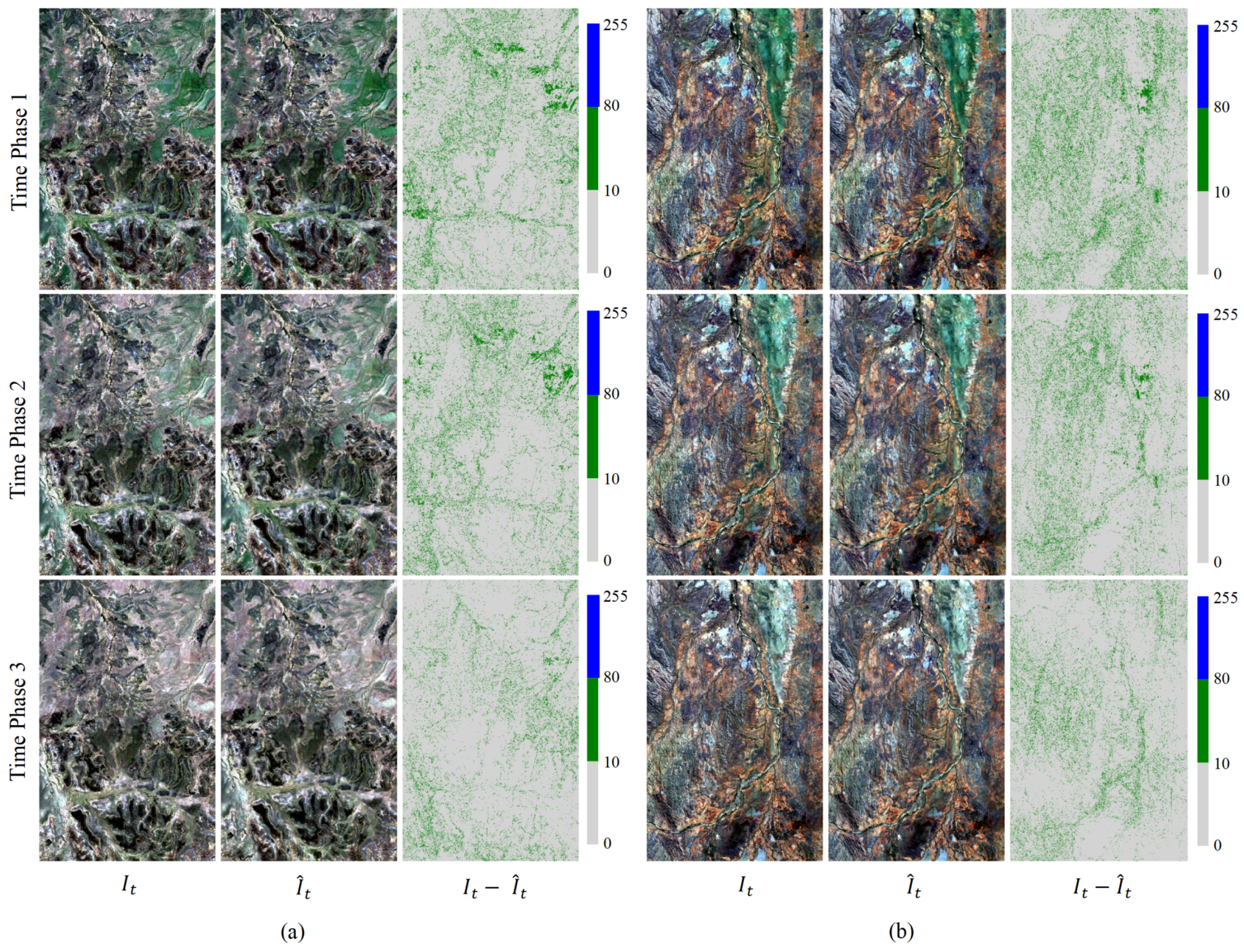
We conducted pixel error analysis on the interpolation results. We linearly mapped the pixel value range from [0, 65,535] to [0, 255]. Subsequently, we computed the pixel error between the interpolated result and the actual image. A pixel error range of [0, 10] indicates low error, (10, 80] indicates medium error, and (80, 255] indicates high error.

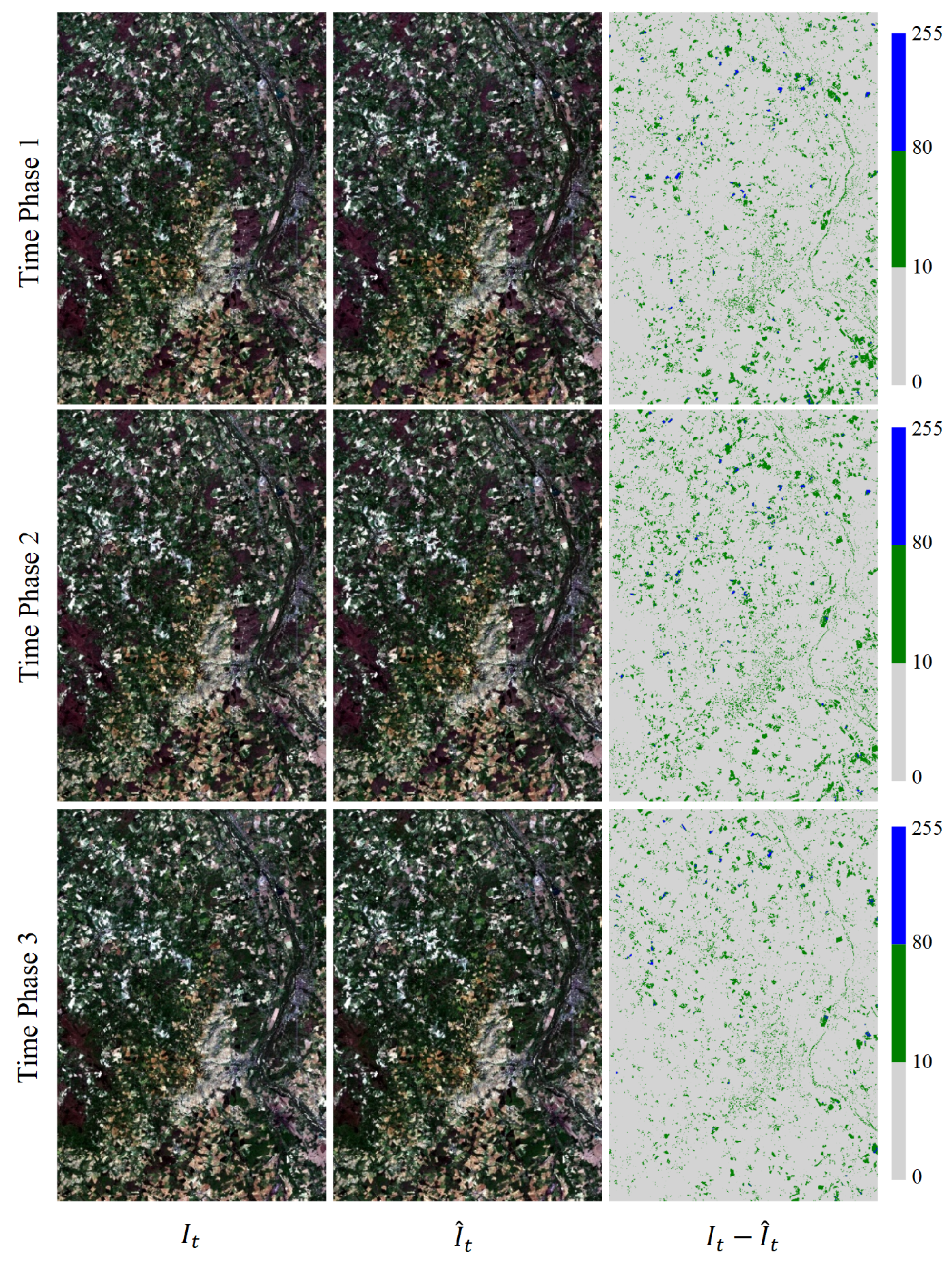
The visual effect maps of the actual images from the three time phases of Experiment 2 for the Landsat-8 and Sentinel-2 test datasets, the visual effect maps of the interpolated results, and the pixel error maps are depicted in Figure 6 and Figure 7. These figures illustrate that the spatial features of the test results from the three time phases of the proposed method across different datasets align closely with those of the corresponding actual images. Most of the pixel errors are concentrated in the range of 0 to 10, with a minor proportion of pixel errors falling in the range of 10 to 80, and very few pixel errors in the range of 80 to 255. This outcome underscores the robust generalization capability of our method.

3.3.2. Evaluation of Point Spectrum

To showcase the predictive capability of our method with respect to feature spectra, we conducted tests on point spectra. Specifically, to mitigate the influence of chance, we randomly selected 100 test points from each of the two test datasets. We then computed the average of these points in each spectral channel for comparison with the actual values.

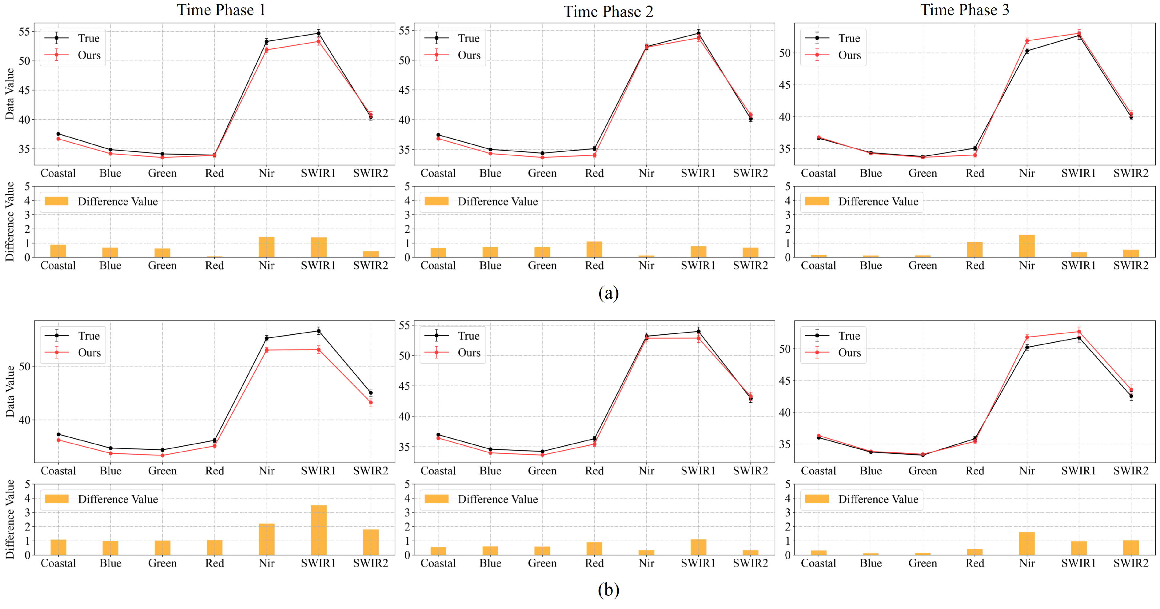
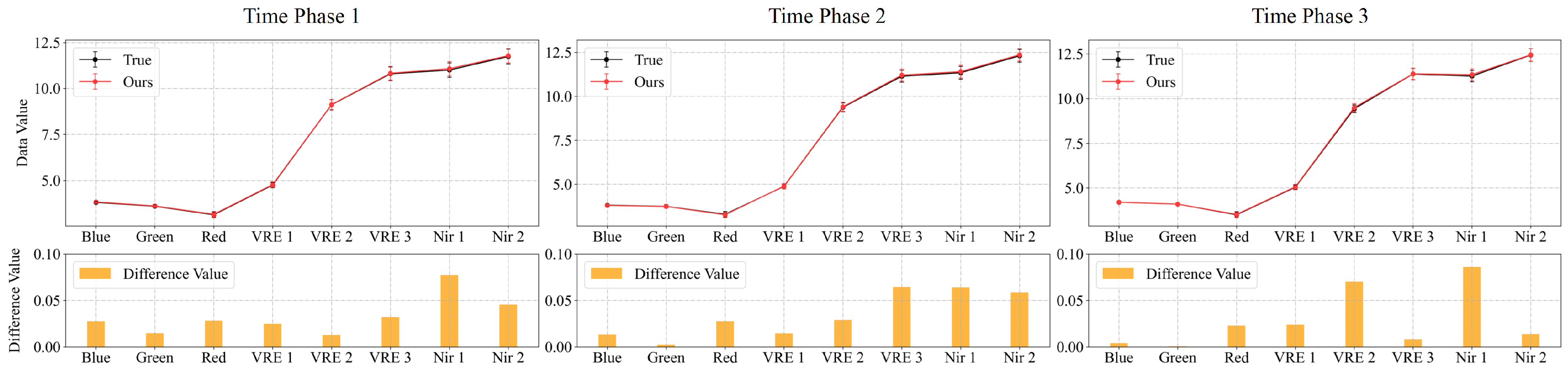
The point spectral maps of the results from Experiment 2 for the Landsat-8 and Sentinel-2 test datasets are depicted in Figure 8 and Figure 9. These maps demonstrate that the point spectral features of our method’s interpolated results across the three time phases in different datasets align closely with those of the corresponding actual images. The interpolation results are within a range of 4 from the actual image in each spectral channel for the Landsat-8 test dataset and within 0.1 for the Sentinel-2 test dataset. This outcome indirectly validates the effectiveness of our method in applying the spectral loss function.

3.3.3. Comparative Experiments

To substantiate the superior performance of our method over existing approaches, we selected the linear method (Linear) and three deep learning methods—Unet [31], Super SloMo [30], and IFRNet [32] for comparative analysis. The Linear method is frequently employed as a baseline in comparative tests of sequential image interpolation, while the other three methods have recently demonstrated good performance in sequence image interpolation.

Table 5. Quantitative comparison of multi-temporal sequential image interpolation results on the Landsat-8 dataset. For each indicator, the results in bold are the best results and those marked with * are the second best results. Time phases 1, 2, and 3 represent the experimental results for the middle three time phases t = 0.25, 0.50, and 0.75. Arrows ↓ and ↑ stand for smaller is better and bigger is better.

Experiment	Method	Time Phase 1			Time Phase 2			Time Phase 3
ID		RMSE↓	PSNR↑	SSIM↑	RMSE↓	PSNR↑	SSIM↑	RMSE↓	PSNR↑	SSIM↑
1	Linear	9.357	29.154	0.957	9.225	29.330	0.958	9.106	29.513	0.959
	Unet [31]	10.997	27.980	0.942	10.074	28.769	0.949	9.823	29.028	0.955
	Super SloMo [30]	8.996	29.550	0.961	8.813	29.766	0.963	8.584	30.102	0.966
	IFRNet [32]	8.140 *	30.197 *	0.971 *	7.892 *	30.367 *	0.977	7.642 *	30.734 *	0.975 *
	Ours	7.860	30.383	0.972	7.216	31.359	0.972 *	7.069	31.736	0.978
2	Linear	8.448	30.091	0.967	8.395	30.224	0.972	6.528	32.299	0.979
	Unet [31]	10.763	28.091	0.947	9.830	28.948	0.954	9.579	29.070	0.957
	Super SloMo [30]	8.178	30.329	0.971	8.372	30.168	0.969	6.216	32.703	0.980 *
	IFRNet [32]	7.384 *	31.173 *	0.977 *	6.900 *	31.912 *	0.979 *	5.696 *	33.434 *	0.984
	Ours	6.770	31.940	0.980	6.275	32.732	0.981	5.532	33.752	0.984
3	Linear	8.588	30.038	0.965	8.734	29.804	0.963	7.192	31.500	0.977
	Unet [31]	9.304	29.228	0.958	9.254	29.298	0.958	8.862	29.740	0.961
	Super SloMo [30]	7.841	30.401	0.974	7.800	30.446	0.975	6.928	31.738	0.979
	IFRNet [32]	6.884 *	31.931 *	0.979 *	7.077 *	31.655 *	0.978 *	6.196 *	33.150 *	0.982 *
	Ours	6.154	33.375	0.983	6.268	33.112	0.981	5.648	33.453	0.984
4	Linear	8.618	29.858	0.964	8.976	29.674	0.961	8.509	30.163	0.967
	Unet [31]	9.276	29.229	0.958	9.344	29.192	0.957	9.179	29.458	0.959
	Super SloMo [30]	7.130 *	30.981	0.976	7.396	31.111	0.976 *	7.998	30.279	0.971
	IFRNet [32]	7.130 *	31.545 *	0.978 *	6.910 *	31.910 *	0.979	7.127 *	31.615 *	0.978 *
	Ours	6.377	32.436	0.980	6.889	31.917	0.979	6.210	33.119	0.980

and

Table 6. Quantitative comparison of multi-temporal sequential image interpolation results on the Sentinel-2 dataset. For each indicator, the results in bold are the best results and those marked with * are the second best results. Time phases 1, 2, and 3 represent the experimental results for the middle three time phases t = 0.25, 0.50, and 0.75. Arrows ↓ and ↑ stand for smaller is better and bigger is better.

Experiment	Method	Time Phase 1			Time Phase 2			Time Phase 3
ID		RMSE↓	PSNR↑	SSIM↑	RMSE↓	PSNR↑	SSIM↑	RMSE↓	PSNR↑	SSIM↑
1	Linear	11.029	28.083	0.959	12.031	27.389	0.942	11.501	27.633	0.944
	Unet [31]	9.211	29.751	0.963	9.308	29.745	0.962	10.167	28.557	0.961 *
	Super SloMo [30]	10.898	28.234	0.960	11.109	27.998	0.959	10.485	28.524	0.961 *
	IFRNet [32]	8.368 *	30.754 *	0.970 *	9.969	28.949	0.961 *	9.472 *	29.709 *	0.961 *
	Ours	7.486	31.411	0.975	9.821 *	29.558 *	0.960	9.140	29.820	0.965
2	Linear	11.961	27.458	0.943	12.924	26.499	0.940	11.135	27.765	0.959
	Unet [31]	9.575	29.948 *	0.959	9.124	29.854	0.966 *	7.888 *	31.104 *	0.973 *
	Super SloMo [30]	11.276	27.996	0.948	10.157	28.816	0.960	10.313	28.536	0.961
	IFRNet [32]	9.412 *	29.733	0.962 *	9.028 *	29.980 *	0.966 *	8.821	29.858	0.970
	Ours	8.597	30.856	0.967	8.471	30.664	0.970	7.237	31.873	0.978
3	Linear	11.295	27.914	0.948	11.822	27.466	0.943	14.500	25.598	0.932
	Unet [31]	10.126	29.110	0.960	10.160	28.653	0.960 *	12.852	26.000	0.940 *
	Super SloMo [30]	10.868	28.241	0.960	10.826	28.323	0.960 *	13.053	26.403	0.936
	IFRNet [32]	9.230 *	29.747 *	0.963 *	9.670 *	29.707 *	0.959	11.911 *	27.460 *	0.943
	Ours	8.962	30.123	0.967	9.194	29.787	0.964	11.809	27.501	0.943
4	Linear	11.440	27.687	0.946	13.121	26.249	0.936	11.392	27.835	0.947
	Unet [31]	9.417	29.721 *	0.962	11.158	28.170 *	0.960 *	8.352	30.531	0.968
	Super SloMo [30]	10.111	29.207	0.960	12.191	26.936	0.941	9.771	29.690	0.959
	IFRNet [32]	9.348 *	29.679	0.963 *	10.933 *	28.149	0.960 *	8.282 *	30.791 *	0.971
	Ours	8.010	30.901	0.970	9.126	29.853	0.966	7.999	30.903	0.970 *

present the quantitative evaluations of the five methods across three metrics—RMSE, PSNR, and SSIM—for the three time phases. On the test datasets of Landsat-8 and Sentinel-2, our method outperforms others in terms of indicator values. Specifically, our method achieves a 7.54% lower RMSE compared to other approaches. Furthermore, only our method surpasses the performance of IFRNet on the Landsat-8 dataset. Similarly, on the Sentinel-2 dataset, only our method outperforms IFRNet and Unet.

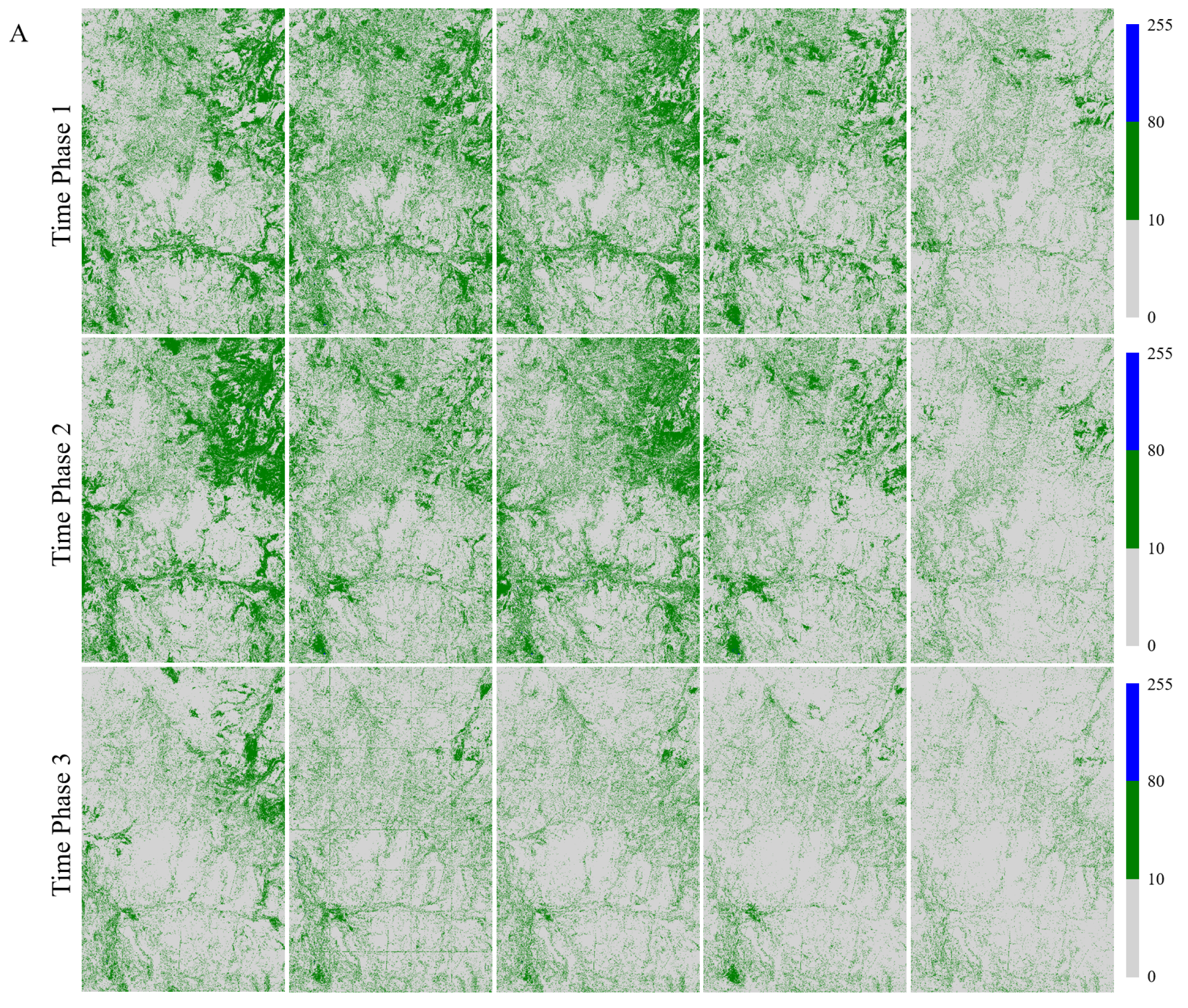
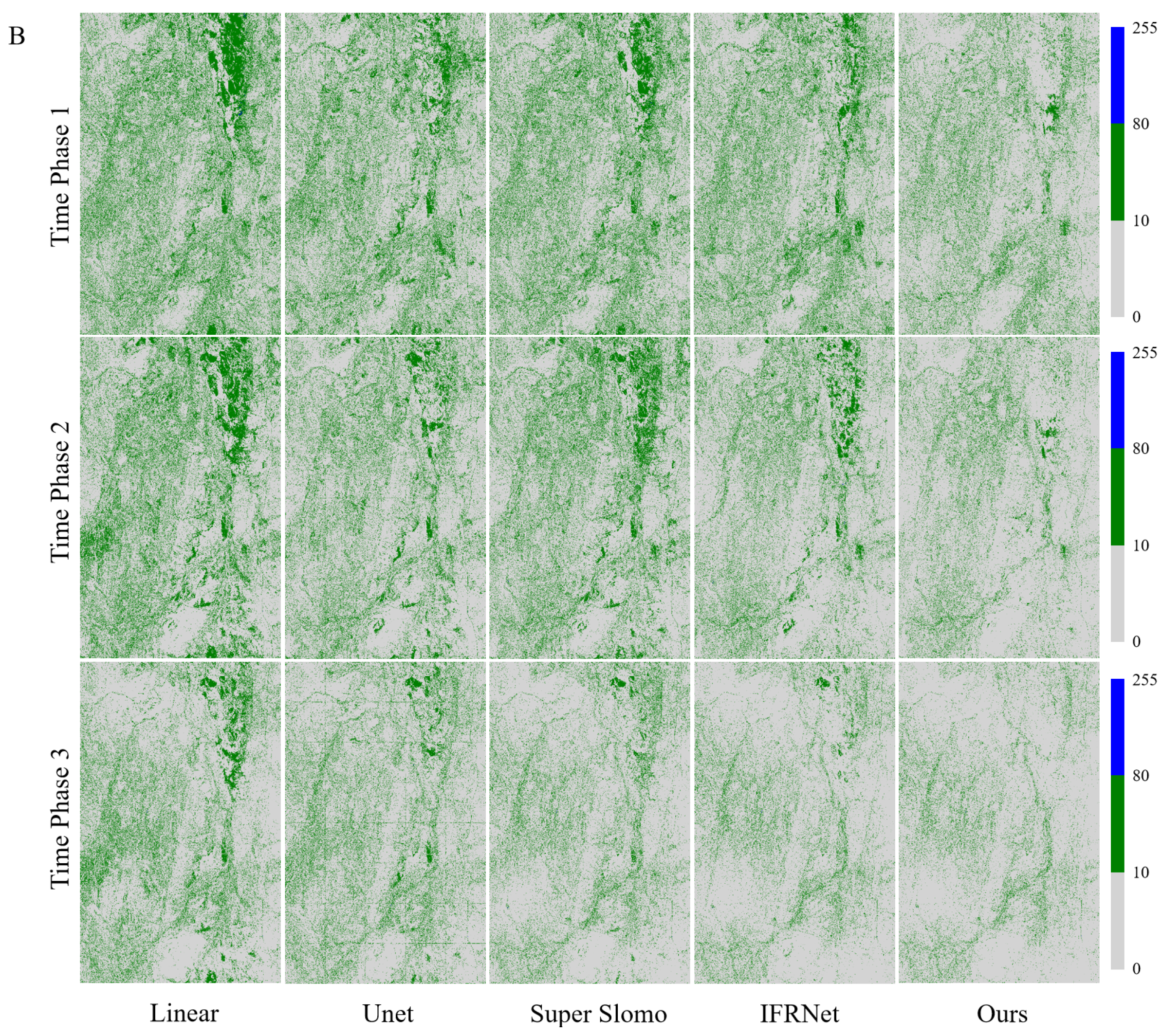
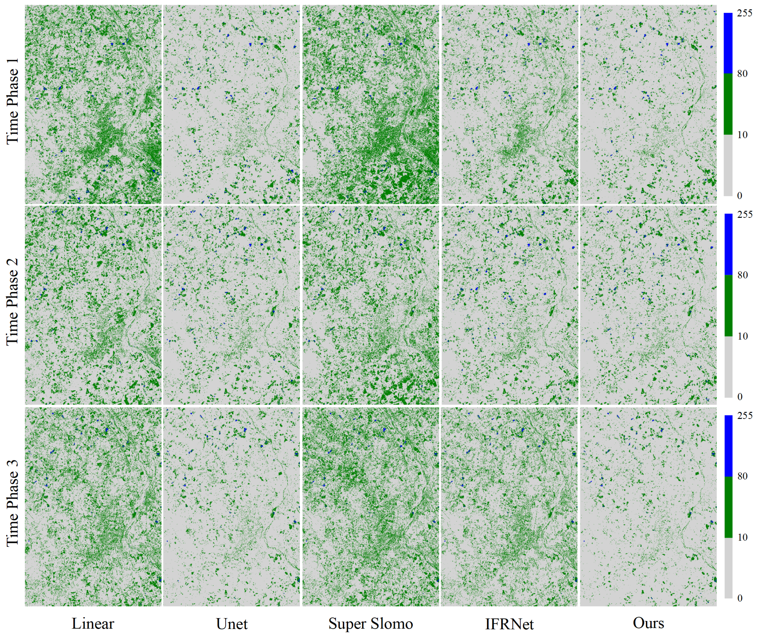
The pixel error maps of the comparative experiments from Experiment 2 on the Landsat-8 satellite dataset are depicted in Figure 10 and Figure 11. These figures reveal that the pixel error between our method’s interpolation results and the actual image across all three time phases is lower than that of the other four methods on the test datasets. Both the Linear and Super SloMo methods exhibit substantial pixel errors. Moreover, other methods display large errors in image areas with extensive vegetation coverage, as these areas undergo more changes over time. In contrast, our method yields lower pixel errors than other methods due to the incorporation of optical flow learning and prediction, enabling our method to accurately capture object changes and thus precisely predict pixel positions.

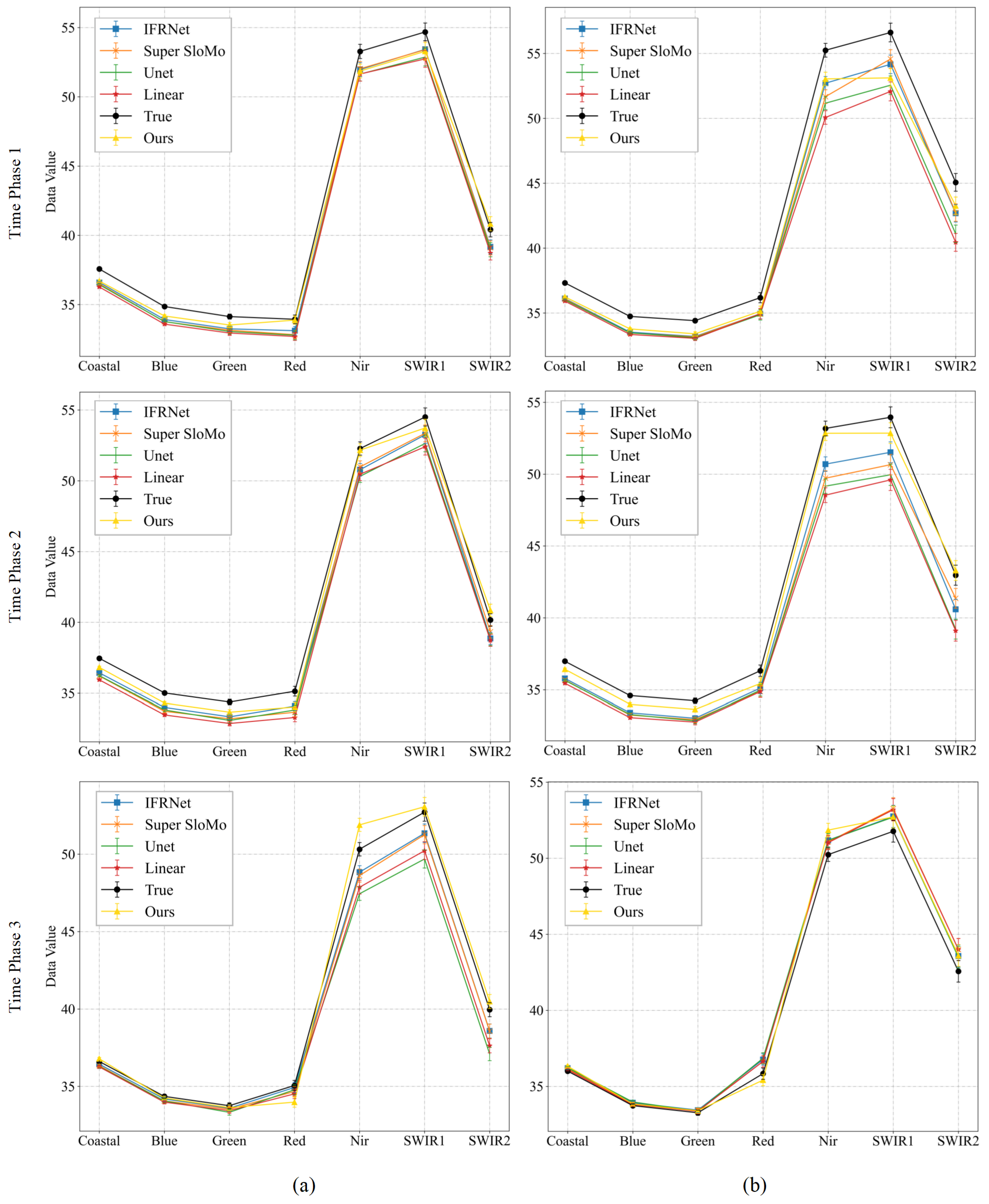
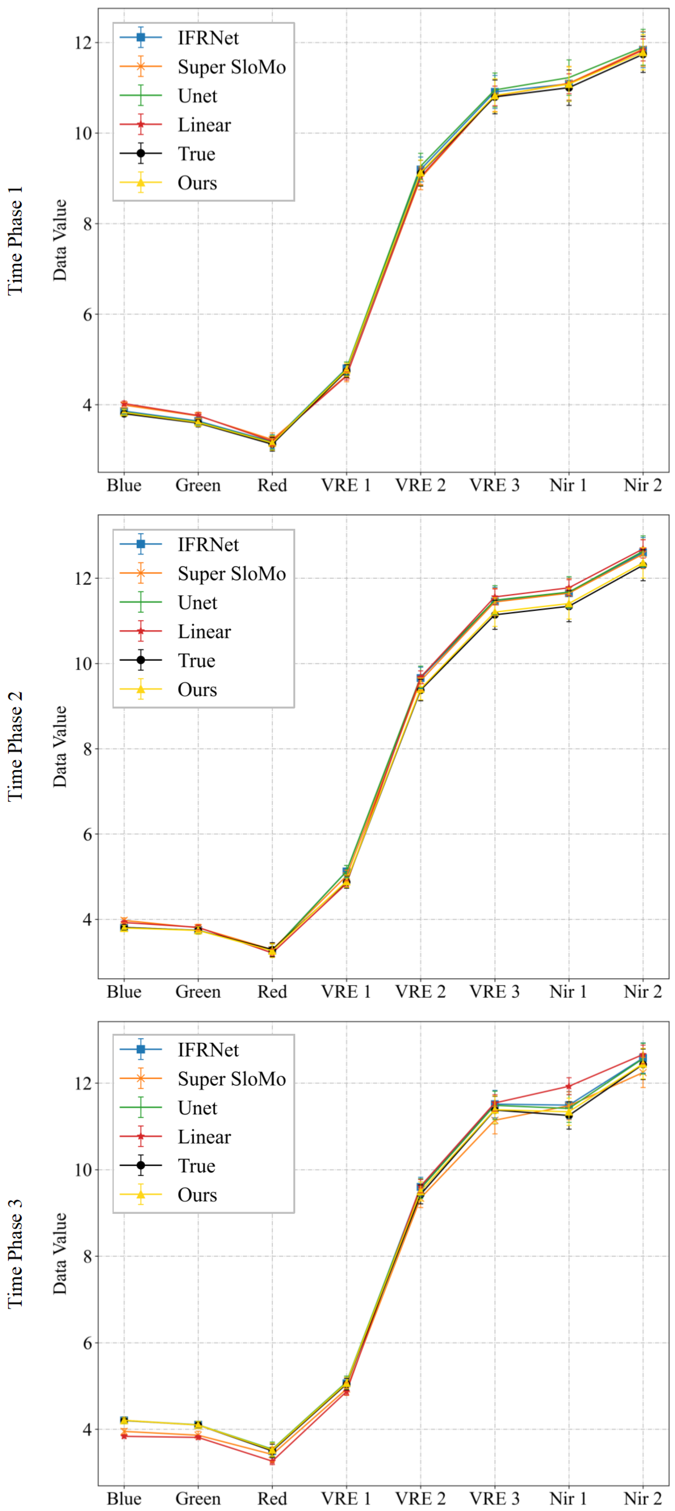
Similarly, we computed the interpolated results of these five methods in comparison with the actual images based on the spectral values at 100 random points from Experiment 2 on the Landsat-8 satellite dataset. The results are shown in Figure 12 and Figure 13. They indicate that, in the test datasets of two time series datasets, the spectral features of our method’s interpolated results across the three time phases at the specified point are closer to the actual spectral features than those of the other four methods.

4. Discussion

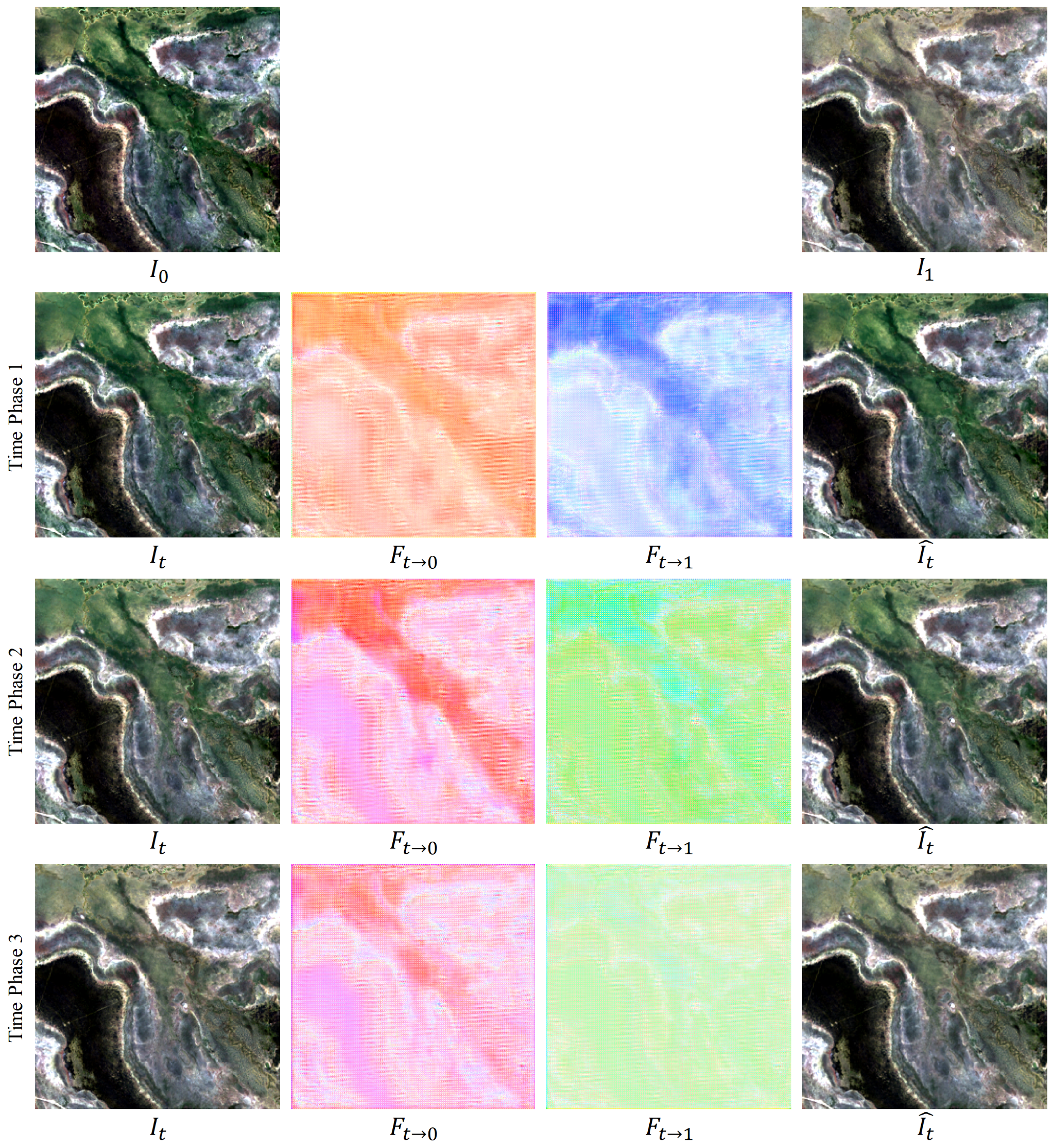
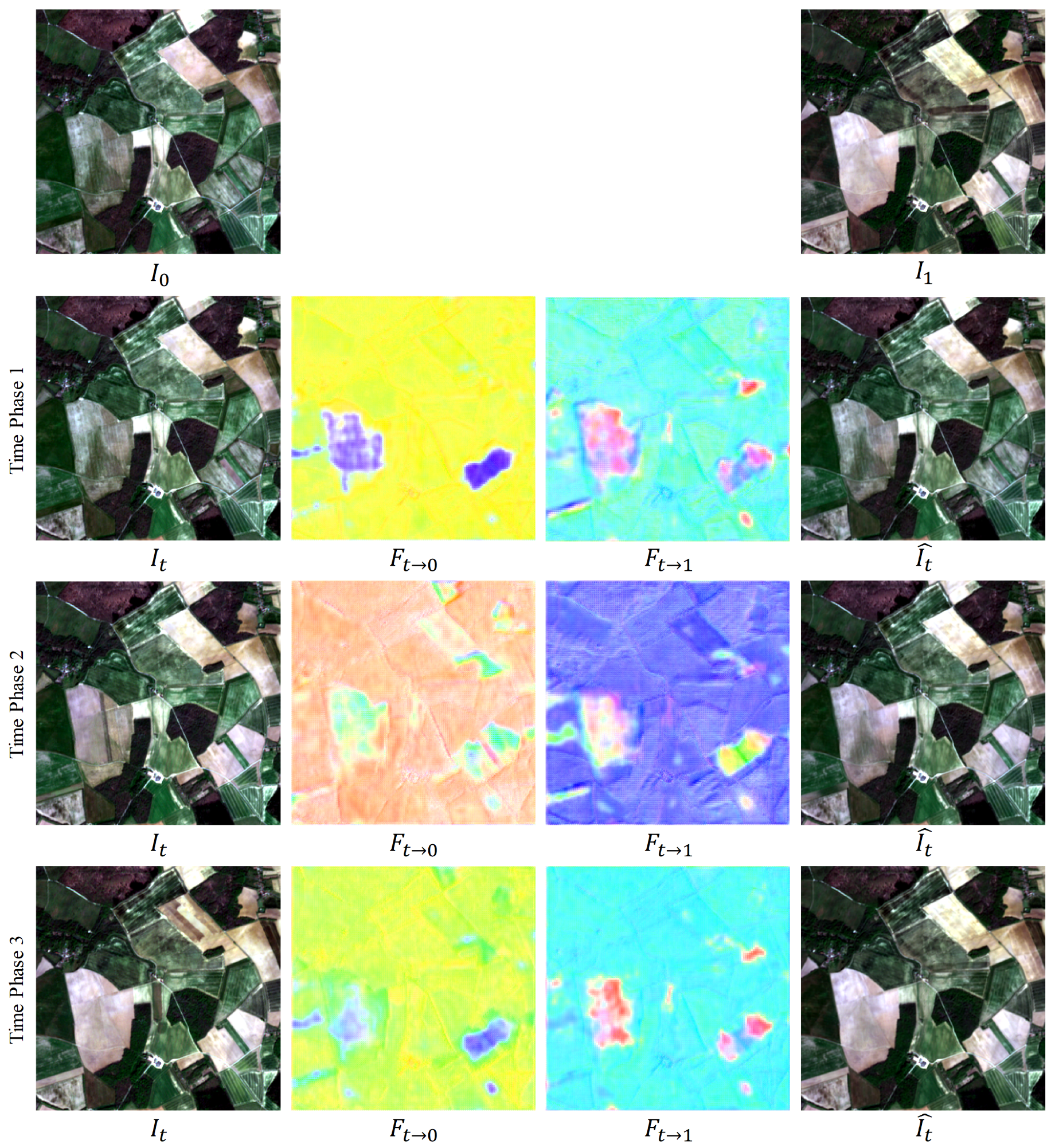
To illustrate the efficacy of incorporating optical flow learning in our deep learning method, we selected a 256 × 256 block from each of the two test datasets to display the intermediate three temporal optical flow and interpolation results. As depicted in Figure 14 and Figure 15, our model accurately predicted the intermediate optical flow by jointly refining the intermediate optical flow and the intermediate features at multiple scales. The bi-directional optical flows have the capability to capture the changes in object pixels between the images from two input time phases. Moreover, our method predicts images that are visually indistinguishable from actual images, owing to the multi-channel occlusion information mask and the multi-channel detail compensation information residuals.

Furthermore, we provide a detailed analysis of why our method surpasses the other four techniques. The Linear method focuses solely on the pixel values to be interpolated in the images from the preceding and subsequent time phases, without taking into account the spatial and spectral features of the images. Unet considers the spatial features of the images from the preceding and subsequent time phases, but neglects the spectral features and the pixel correspondences in the temporal images (optical flow). Both Super SloMo and IFRNet take into account the spatial features of the images and the pixel correspondences in the temporal images. However, Super SloMo separates the refinement of the optical and spatial features into two phases, resulting in a disconnection between the two. IFRNet performs a joint refinement of the optical flow and the spatial features, but its interpolation effect is superior for RGB images and inferior for multispectral satellite images. In contrast, our proposed method excels at handling multispectral satellite imagery by extending the number of detail-compensated residual channels to match the number of spectra and implementing a spectral loss function to enhance the supervision of spectral learning.

5. Conclusions

Inspired by video frame interpolation, this paper proposed a method for satellite sequence image interpolation. This method leverages a multi-layer convolutional network to learn the intermediate optical flow and intermediate features of the image. It predicts the precise positions of pixels and complex spatial features, ultimately yielding a highly accurate image for the intermediate time phase. The key conclusions of this paper can be summarized as follows:

(1)

Our proposed method predicts images for intermediate time phases based on optical flow and intermediate features. It excels at capturing the intermediate optical flow and integrating the intermediate features to produce superior interpolated images. Our research offers a novel paradigm for interpolating satellite image sequences of complex objects.

(2)

Thanks to the multi-channel mask structure of occlusion information and the spectral loss function in our model, our approach yields lower interpolation errors across all four seasons: spring, summer, autumn, and winter. Specifically, our method’s results on the test dataset exhibit a 7.54% RMSE compared to other approaches.

In future work, we aim to explore the utilization of information from images in multiple time phases of a time series to guide the generation of images in intermediate temporal phases, rather than relying solely on information from the images of the preceding and subsequent time phases of the image to be interpolated.

References

- Guo, H.; Wang, L.; Liang, D. Big Earth Data from space: A new engine for Earth science. Sci. Bull. 2016, 61, 505–513. [Google Scholar] [CrossRef]
- Vatsavai, R.R.; Ganguly, A.; Chandola, V.; Stefanidis, A.; Klasky, S.; Shekhar, S. Spatiotemporal data mining in the era of big spatial data: Algorithms and applications. In Proceedings of the 1st ACM SIGSPATIAL International Workshop on Analytics for Big Geospatial Data, Redondo Beach, CA, USA, 6 November 2012; pp. 1–10. [Google Scholar]
- Salmon, B.P.; Olivier, J.C.; Wessels, K.J.; Kleynhans, W.; van den Bergh, F.; Steenkamp, K.C. Unsupervised Land Cover Change Detection: Meaningful Sequential Time Series Analysis. IEEE J. Sel. Top. Appl. Earth Obs. Remote Sens. 2011, 4, 327–335. [Google Scholar] [CrossRef]
- Chen, L.; Jin, Z.; Michishita, R.; Cai, J.; Yue, T.; Chen, B.; Xu, B. Dynamic monitoring of wetland cover changes using time-series remote sensing imagery. Ecol. Inform. 2014, 24, 17–26. [Google Scholar] [CrossRef]
- Li, Q.; Wang, C.; Zhang, B.; Lu, L. Object-Based Crop Classification with Landsat-MODIS Enhanced Time-Series Data. Remote Sens. 2015, 7, 16091–16107. [Google Scholar] [CrossRef]
- Li, M.; Zhang, L.; Ding, C.; Li, W.; Luo, H.; Liao, M.; Xu, Q. Retrieval of historical surface displacements of the Baige landslide from time-series SAR observations for retrospective analysis of the collapse event. Remote Sens. Environ. 2020, 240, 111695. [Google Scholar] [CrossRef]
- Marghany, M. Nonlinear Ocean Dynamics: Synthetic Aperture Radar; Elsevier: Amsterdam, The Netherlands, 2021. [Google Scholar]
- Shen, H.; Li, X.; Cheng, Q.; Zeng, C.; Yang, G.; Li, H.; Zhang, L. Missing information reconstruction of remote sensing data: A technical review. IEEE Geosci. Remote Sens. Mag. 2015, 3, 61–85. [Google Scholar] [CrossRef]
- Li, R.; Zhang, X.; Liu, B. Review on Filtering and Reconstruction Algorithms of Remote Sensing Time Series Data. J. Remote Sens. 2009, 13, 335–341. [Google Scholar]
- Marghany, M. Remote Sensing and Image Processing in Mineralogy; CRC Press: Boca Raton, FL, USA, 2022. [Google Scholar]
- Vandal, T.J.; Nemani, R.R. Temporal interpolation of geostationary satellite imagery with optical flow. IEEE Trans. Neural Netw. Learn. Syst. 2021, 34, 3245–3254. [Google Scholar] [CrossRef]
- Dosovitskiy, A.; Brox, T. Generating images with perceptual similarity metrics based on deep networks. In Proceedings of the Advances in Neural Information Processing Systems 29: Annual Conference on Neural Information Processing Systems 2016, Barcelona, Spain, 5–10 December 2016; Volume 29. [Google Scholar]
- Raya, S.P.; Udupa, J.K. Shape-based interpolation of multidimensional objects. IEEE Trans. Med. Imaging 1990, 9, 32–42. [Google Scholar] [CrossRef]
- Li, J.; Hong, D.; Gao, L.; Yao, J.; Zheng, K.; Zhang, B.; Chanussot, J. Deep learning in multimodal remote sensing data fusion: A comprehensive review. Int. J. Appl. Earth Obs. Geoinf. 2022, 112, 102926. [Google Scholar] [CrossRef]
- Vivone, G.; Dalla Mura, M.; Garzelli, A.; Restaino, R.; Scarpa, G.; Ulfarsson, M.O.; Alparone, L.; Chanussot, J. A New Benchmark Based on Recent Advances in Multispectral Pansharpening: Revisiting Pansharpening with Classical and Emerging Pansharpening Methods. IEEE Geosci. Remote Sens. Mag. 2021, 9, 53–81. [Google Scholar] [CrossRef]
- Zhang, W.; Tang, P.; Zhao, L. Remote Sensing Image Scene Classification Using CNN-CapsNet. Remote Sens. 2019, 11, 494. [Google Scholar] [CrossRef]
- Bazi, Y.; Bashmal, L.; Rahhal, M.M.A.; Dayil, R.A.; Ajlan, N.A. Vision Transformers for Remote Sensing Image Classification. Remote Sens. 2021, 13, 516. [Google Scholar] [CrossRef]
- Ma, W.; Li, N.; Zhu, H.; Jiao, L.; Tang, X.; Guo, Y.; Hou, B. Feature Split-Merge-Enhancement Network for Remote Sensing Object Detection. IEEE Trans. Geosci. Remote Sens. 2022, 60, 5616217. [Google Scholar] [CrossRef]
- Li, X.; Deng, J.; Fang, Y. Few-Shot Object Detection on Remote Sensing Images. IEEE Trans. Geosci. Remote Sens. 2022, 60, 5601614. [Google Scholar] [CrossRef]
- Yu, D.; Ji, S. A New Spatial-Oriented Object Detection Framework for Remote Sensing Images. IEEE Trans. Geosci. Remote Sens. 2022, 60, 4407416. [Google Scholar] [CrossRef]
- Li, T.; Gu, Y. Progressive Spatial–Spectral Joint Network for Hyperspectral Image Reconstruction. IEEE Trans. Geosci. Remote Sens. 2022, 60, 5507414. [Google Scholar] [CrossRef]
- Sun, X.; Wang, P.; Lu, W.; Zhu, Z.; Lu, X.; He, Q.; Li, J.; Rong, X.; Yang, Z.; Chang, H.; et al. RingMo: A Remote Sensing Foundation Model with Masked Image Modeling. IEEE Trans. Geosci. Remote Sens. 2023, 61, 5612822. [Google Scholar] [CrossRef]
- Yao, F.; Lu, W.; Yang, H.; Xu, L.; Liu, C.; Hu, L.; Yu, H.; Liu, N.; Deng, C.; Tang, D.; et al. RingMo-Sense: Remote Sensing Foundation Model for Spatiotemporal Prediction via Spatiotemporal Evolution Disentangling. IEEE Trans. Geosci. Remote Sens. 2023, 61, 5620821. [Google Scholar] [CrossRef]
- Niklaus, S.; Mai, L.; Liu, F. Video frame interpolation via adaptive convolution. In Proceedings of the IEEE Conference on Computer Vision and Pattern Recognition, Honolulu, HI, USA, 21–26 July 2017; pp. 670–679. [Google Scholar]
- Jin, X.; Tang, P.; Houet, T.; Corpetti, T.; Alvarez-Vanhard, E.G.; Zhang, Z. Sequence image interpolation via separable convolution network. Remote Sens. 2021, 13, 296. [Google Scholar] [CrossRef]
- Peleg, T.; Szekely, P.; Sabo, D.; Sendik, O. Im-net for high resolution video frame interpolation. In Proceedings of the IEEE/CVF Conference on Computer Vision and Pattern Recognition, Long Beach, CA, USA, 15–20 June 2019; pp. 2398–2407. [Google Scholar]
- Cassisa, C.; Simoens, S.; Prinet, V.; Shao, L. Sub-grid physical optical flow for remote sensing of sandstorm. In Proceedings of the 2010 IEEE International Geoscience and Remote Sensing Symposium, IEEE, Honolulu, HI, USA, 25–30 July 2010; pp. 2230–2233. [Google Scholar]
- Deng, C.; Cao, Z.; Fang, Z.; Yu, Z. Ship detection from optical satellite image using optical flow and saliency. In Proceedings of the MIPPR 2013: Remote Sensing Image Processing, Geographic Information Systems, and Other Applications, SPIE, Wuhan, China, 26–27 October 2013; Volume 8921, pp. 100–106. [Google Scholar]
- Liu, Z.; Yeh, R.A.; Tang, X.; Liu, Y.; Agarwala, A. Video frame synthesis using deep voxel flow. In Proceedings of the IEEE International Conference on Computer Vision, Venice, Italy, 22–29 October 2017; pp. 4463–4471. [Google Scholar]
- Jiang, H.; Sun, D.; Jampani, V.; Yang, M.H.; Learned-Miller, E.; Kautz, J. Super slomo: High quality estimation of multiple intermediate frames for video interpolation. In Proceedings of the IEEE Conference on Computer Vision and Pattern Recognition, Salt Lake City, UT, USA, 18–23 June 2018; pp. 9000–9008. [Google Scholar]
- Ronneberger, O.; Fischer, P.; Brox, T. U-Net: Convolutional Networks for Biomedical Image Segmentation. In Proceedings of the Medical Image Computing and Computer-Assisted Intervention—MICCAI 2015, Munich, Germany, 5–9 October 2015; Navab, N., Hornegger, J., Wells, W.M., Frangi, A.F., Eds.; Springer: Cham, Switzerland, 2015; pp. 234–241. [Google Scholar]
- Kong, L.; Jiang, B.; Luo, D.; Chu, W.; Huang, X.; Tai, Y.; Wang, C.; Yang, J. Ifrnet: Intermediate feature refine network for efficient frame interpolation. In Proceedings of the IEEE/CVF Conference on Computer Vision and Pattern Recognition, New Orleans, LA, USA, 18–24 June 2022; pp. 1969–1978. [Google Scholar]
- He, K.; Zhang, X.; Ren, S.; Sun, J. Delving deep into rectifiers: Surpassing human-level performance on imagenet classification. In Proceedings of the IEEE International Conference on Computer Vision, Santiago, Chile, 7–13 December 2015; pp. 1026–1034. [Google Scholar]
- He, K.; Zhang, X.; Ren, S.; Sun, J. Deep Residual Learning for Image Recognition. In Proceedings of the 2016 IEEE Conference on Computer Vision and Pattern Recognition (CVPR), Las Vegas, NV, USA, 27–30 June 2016; pp. 770–778. [Google Scholar] [CrossRef]
- Zhang, T.; Qi, G.J.; Xiao, B.; Wang, J. Interleaved Group Convolutions. In Proceedings of the 2017 IEEE International Conference on Computer Vision (ICCV), Venice, Italy, 22–29 October 2017; pp. 4383–4392. [Google Scholar] [CrossRef]
- Charbonnier, P.; Blanc-Feraud, L.; Aubert, G.; Barlaud, M. Two deterministic half-quadratic regularization algorithms for computed imaging. In Proceedings of the 1st International Conference on Image Processing, IEEE, Austin, TX, USA, 13–16 November 1994; Volume 2, pp. 168–172. [Google Scholar]
- Grevera, G.J.; Udupa, J.K. Shape-based interpolation of multidimensional grey-level images. IEEE Trans. Med. Imaging 1996, 15, 881–892. [Google Scholar] [CrossRef] [PubMed]
- Luo, K.; Wang, C.; Liu, S.; Fan, H.; Wang, J.; Sun, J. Upflow: Upsampling pyramid for unsupervised optical flow learning. In Proceedings of the IEEE/CVF Conference on Computer Vision and Pattern Recognition, Nashville, TN, USA, 20–25 June 2021; pp. 1045–1054. [Google Scholar]
- Kingma, D.P.; Ba, J. Adam: A method for stochastic optimization. arXiv 2014, arXiv:1412.6980. [Google Scholar]
- Loshchilov, I.; Hutter, F. Sgdr: Stochastic gradient descent with warm restarts. arXiv 2016, arXiv:1608.03983. [Google Scholar]
- Huang, X.; Shi, J.; Yang, J.; Yao, J. Evaluation of color image quality based on mean square error and peak signal-to-noise ratio of color difference. Acta Photonica Sin. 2007, 36, 295–298. [Google Scholar]
- Wang, Z.; Bovik, A.C.; Sheikh, H.R.; Simoncelli, E.P. Image quality assessment: From error visibility to structural similarity. IEEE Trans. Image Process. 2004, 13, 600–612. [Google Scholar] [CrossRef]
Figure 1.
Three instances of remote sensing data that are missing: (a) displays a MODIS instrument failure on the Aqua satellite, which caused about 70% of the data in Aqua MODIS band 6 to be lost; (b) displays a Landsat-7 satellite digital product, where the image had pixel failure due to a malfunctioning Landsat-7 ETM+ on-board scanning line corrector; and (c) displays a Landsat-8 OLI_TIRS satellite digital product that is useless for direct use due to its 87.3% cloud coverage.
Figure 2.
Examples of Landsat-8 and Sentinel-2 satellite time series. There are two time series examples for Landsat-8 (a) and Sentinel-2 (b), respectively, with a linear stretch of 2% and a true color synthesis.
Figure 3.
The architecture of the Multi-scale Optical Flow-Intermediate Feature joint Network. The network begins with the encoder , which extracts the four-scale features from the two time-phase images, and . Subsequently, the intermediate optical flows and features are collectively refined by four decoders in an ascending order of scale. The time phase T is input into the decoder . The decoder outputs the bidirectional optical flows, a multi-channel occlusion information mask, and multi-channel detail compensation information residuals, all of which are equal in size to the original image. Finally, these outputs are synthesized with the images from the preceding and subsequent time phases to generate the image at the intermediate time phase T.
Figure 4.
Detailed structure of the residual block used by each sub-decoder. The residual block (b) uses a residual connection (a) as a whole. There are five convolution layers within the residual block, which uses an interleaved convolution (c) at convolution layer 2 and convolution layer 4.
Figure 5.
Distribution of training, testing, and validation samples in our experiment: (a) Landsat-8 and (b) Sentinel-2 images; areas inside blue and red boxes and the remainder of the images show the distribution of testing, validation, and training samples, and training set:validation set:test set = 8:1:1.
Figure 6.
Pixel error map for Experiment 2 of multi-temporal sequence image interpolation for the Landsat-8 satellite dataset. (a,b) are the results of two time series from Experiment 2 of the Landsat-8 satellite dataset. Time phase 1, 2 and 3 represent the experimental results for the middle three time phases t = 0.25, 0.50, and 0.75. , , and represent the real image, the interpolation result, and the pixel error between the two. In the pixel error map, grey, green, and blue represent the absolute value of the pixel difference in the ranges 0–10, 10–80, and 80–255, with larger values representing larger errors.
Figure 7.
Pixel error map for Experiment 2 of multi-temporal sequence image interpolation for the Sentinel-2 satellite dataset. Time phases 1, 2, and 3 represent the experimental results for the middle three time phases t = 0.25, 0.50, and 0.75. , , and represent the real image, the interpolation result, and the pixel error between the two. In the pixel error map, grey, green, and blue represent the absolute value of the pixel difference in the ranges 0–10, 10–80, and 80–255, with larger values representing larger errors.
Figure 8.
Spectral curves map at 100 random points for Experiment 2 of multi-temporal sequence image interpolation for the Landsat-8 satellite dataset. (a,b) are the results of two time series from Experiment 2 of the Landsat-8 satellite dataset. Time phases 1, 2, and 3 represent the experimental results for the middle three time phases t = 0.25, 0.50, and 0.75. For each time phase image, we plotted the average of the spectra of the real image and the interpolated result at 100 random points (True and Ours), and the absolute value of the difference between the two spectra.
Figure 9.
Spectral curves map at 100 random points for Experiment 2 of multi-temporal sequence image interpolation for the Sentinel-2 satellite dataset. Time phases 1, 2, and 3 represent the experimental results for the middle three time phases t = 0.25, 0.50, and 0.75. For each time phase image, we plotted the average of the spectra of the real image and the interpolated result at 100 random points (True and Ours), and the absolute value of the difference between the two spectra.
Figure 10.
Pixel error map for comparative experiments of Experiment 2 for multi-temporal sequence image interpolation on the Landsat-8 satellite dataset. (A,B) are the results of two time series from Experiment 2 of the Landsat-8 satellite dataset. Time phases 1, 2, and 3 represent the experimental results for the middle three time phases t = 0.25, 0.50, and 0.75. In the pixel error map, grey, green, and blue represent the absolute value of the pixel difference in the ranges 0–10, 10–80, and 80–255, with larger values representing larger errors.
Figure 11.
Pixel error map for comparative experiments of Experiment 2 for multi-temporal sequence image interpolation on the Sentinel-2 satellite dataset. Time phases 1, 2, and 3 represent the experimental results for the middle three time phases t = 0.25, 0.50, and 0.75. In the pixel error map, grey, green, and blue represent the absolute value of the pixel difference in the ranges 0–10, 10–80, and 80–255, with larger values representing larger errors.
Figure 12.
Spectral curves map at 100 random points for comparative experiments of Experiment 2 for multi-temporal sequence image interpolation on the Landsat-8 satellite dataset. (a,b) are the results of two time series from Experiment 2 of the Landsat-8 satellite dataset. For each time phase image, we plotted the average of the spectra of the real image and the interpolated results of the five methods at 100 random points.
Figure 13.
Spectral curves map at 100 random points for comparative experiments of Experiment 2 for multi-temporal sequence image interpolation on the Sentinel-2 satellite dataset. For each time phase image, we plotted the average of the spectra of the real image and the interpolated results of the five methods at 100 random points.
Figure 14.
Interpolation results and optical flow visualization of a Landsat-8 image block. The first row displays the images of the previous time phase and the next time phase; the second to third rows are the results of the three intermediate time phases of the images of the previous time phase and the next time phase.
Figure 15.
Interpolation results and optical flow visualization of a Sentinel-2 image block. The first row displays the images of the previous time phase and the next time phase; the second to third rows are the results of the three intermediate time phases of the images of the previous time phase and the next time phase.