


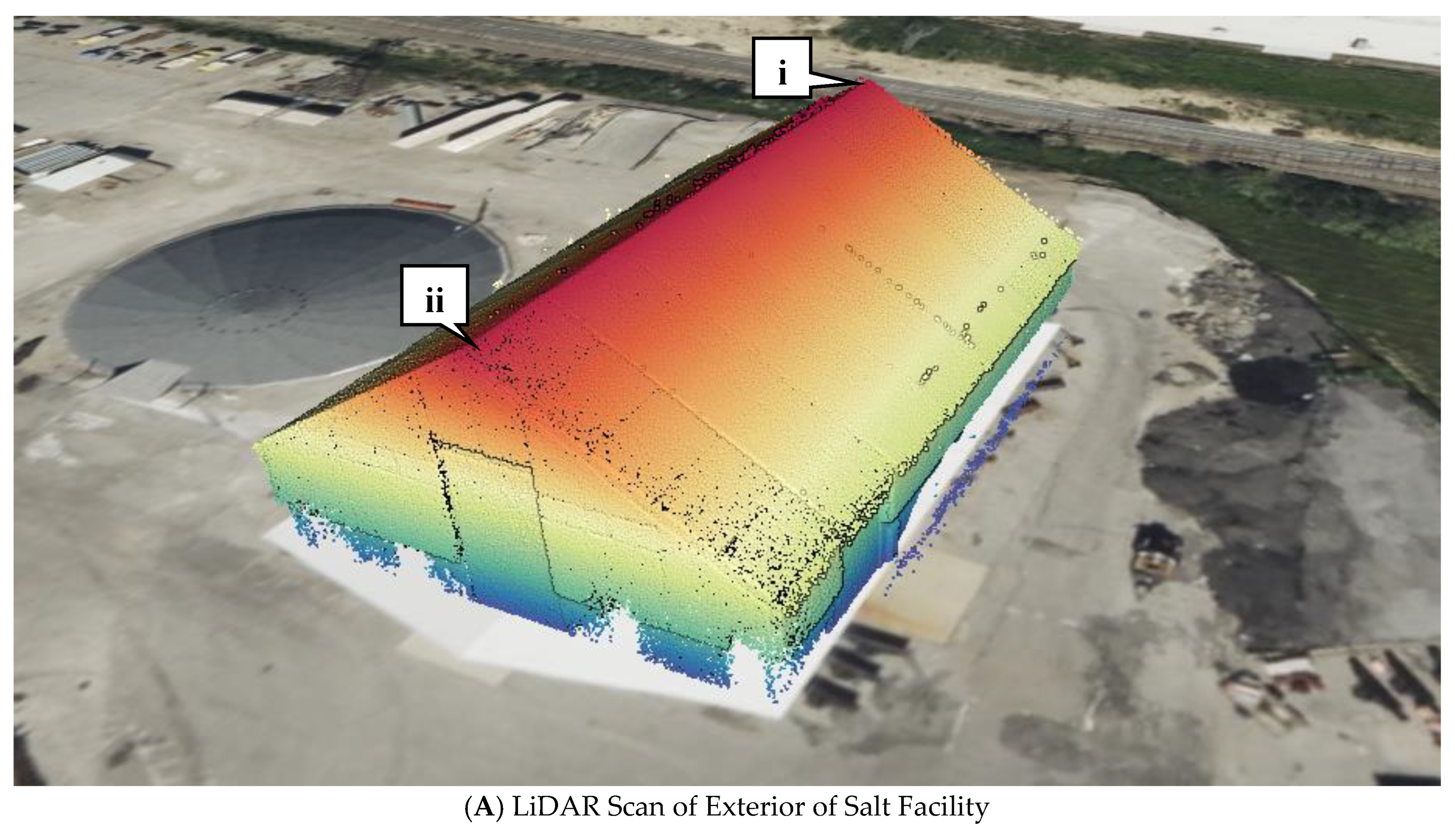
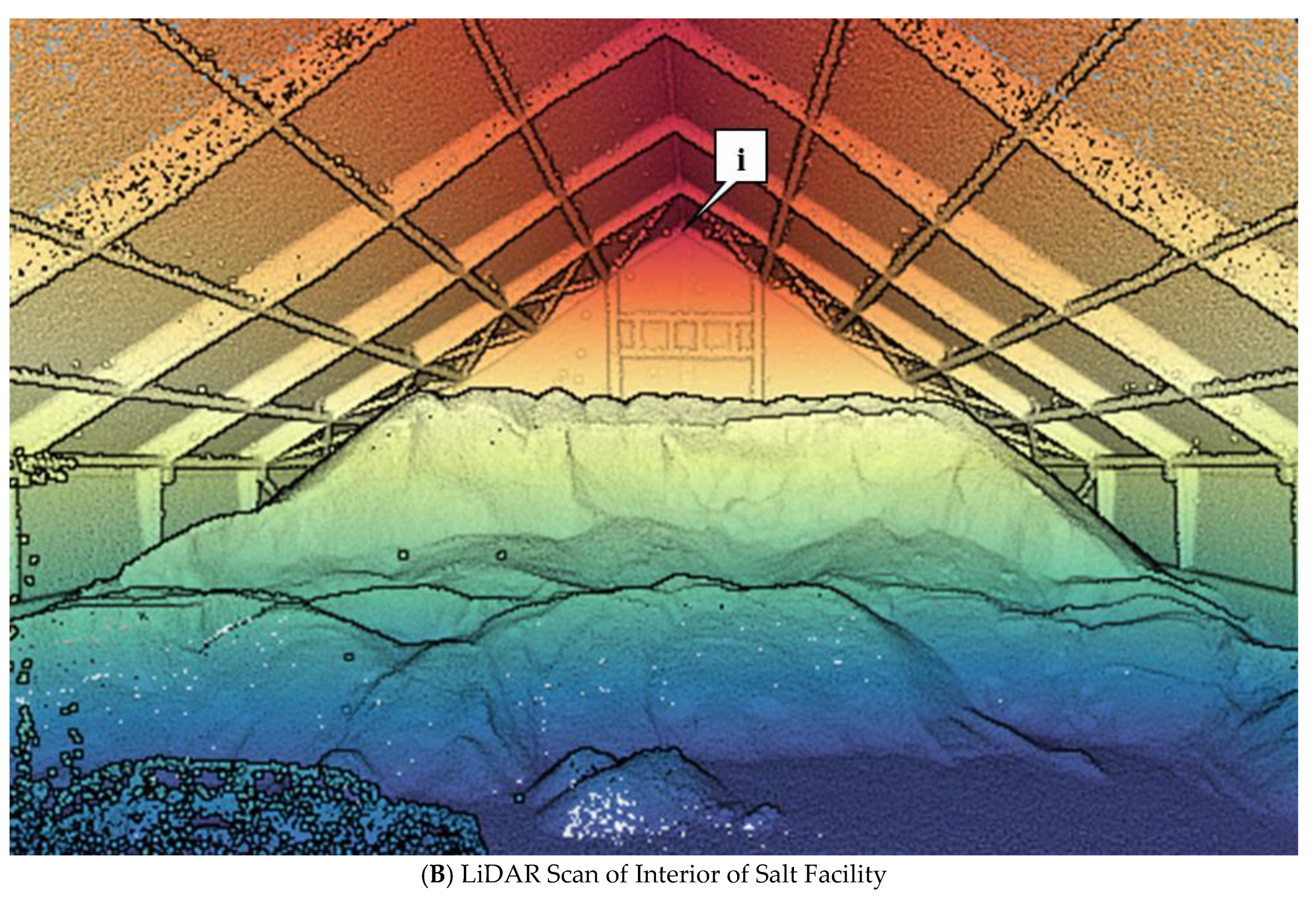
Statewide Implementation of Salt Stockpile Inventory Using LiDAR Measurements: Case Study

 , , and
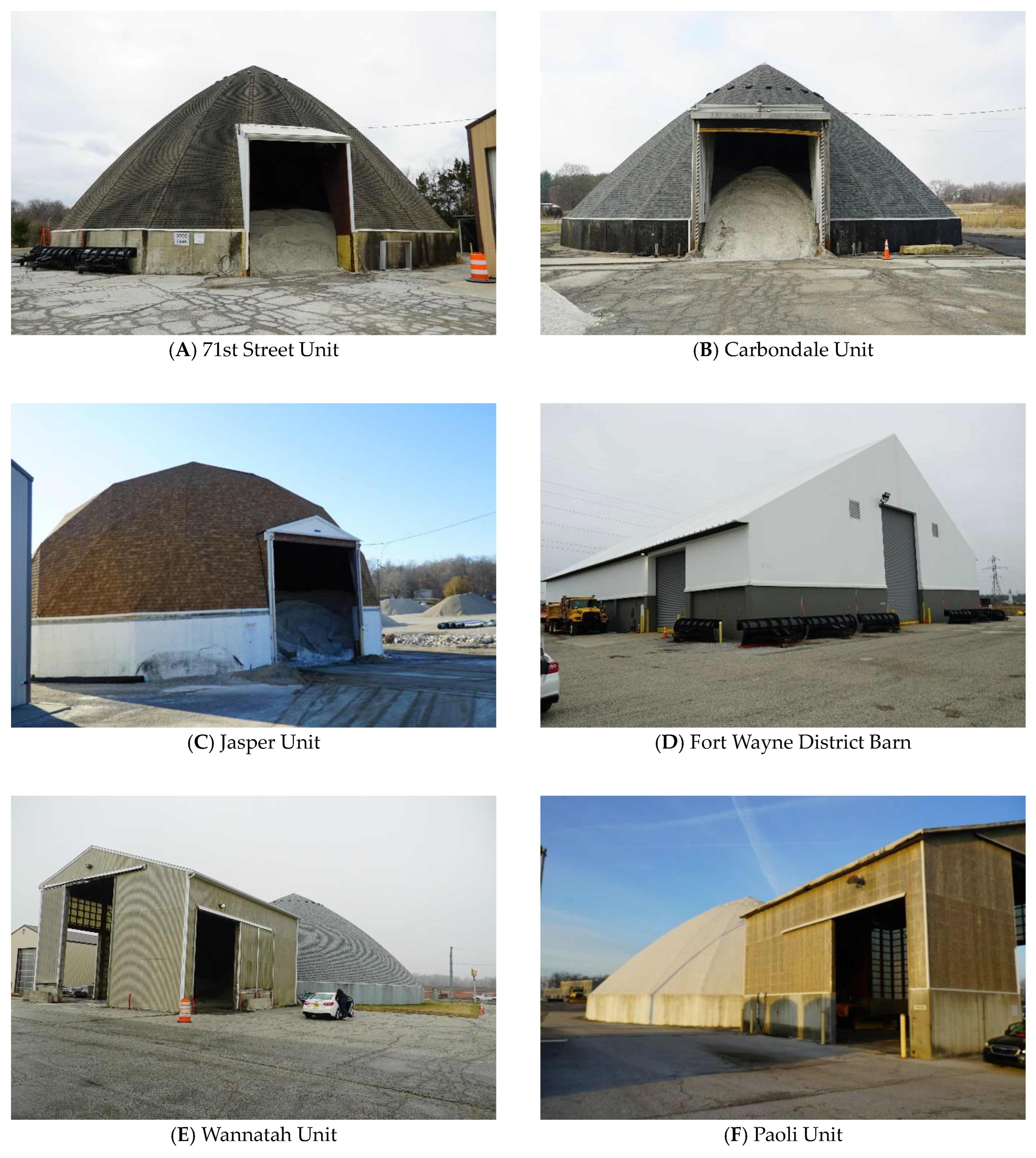
Abstract
:1. Introduction
2. Background and Literature Review
3. Objective and Scope
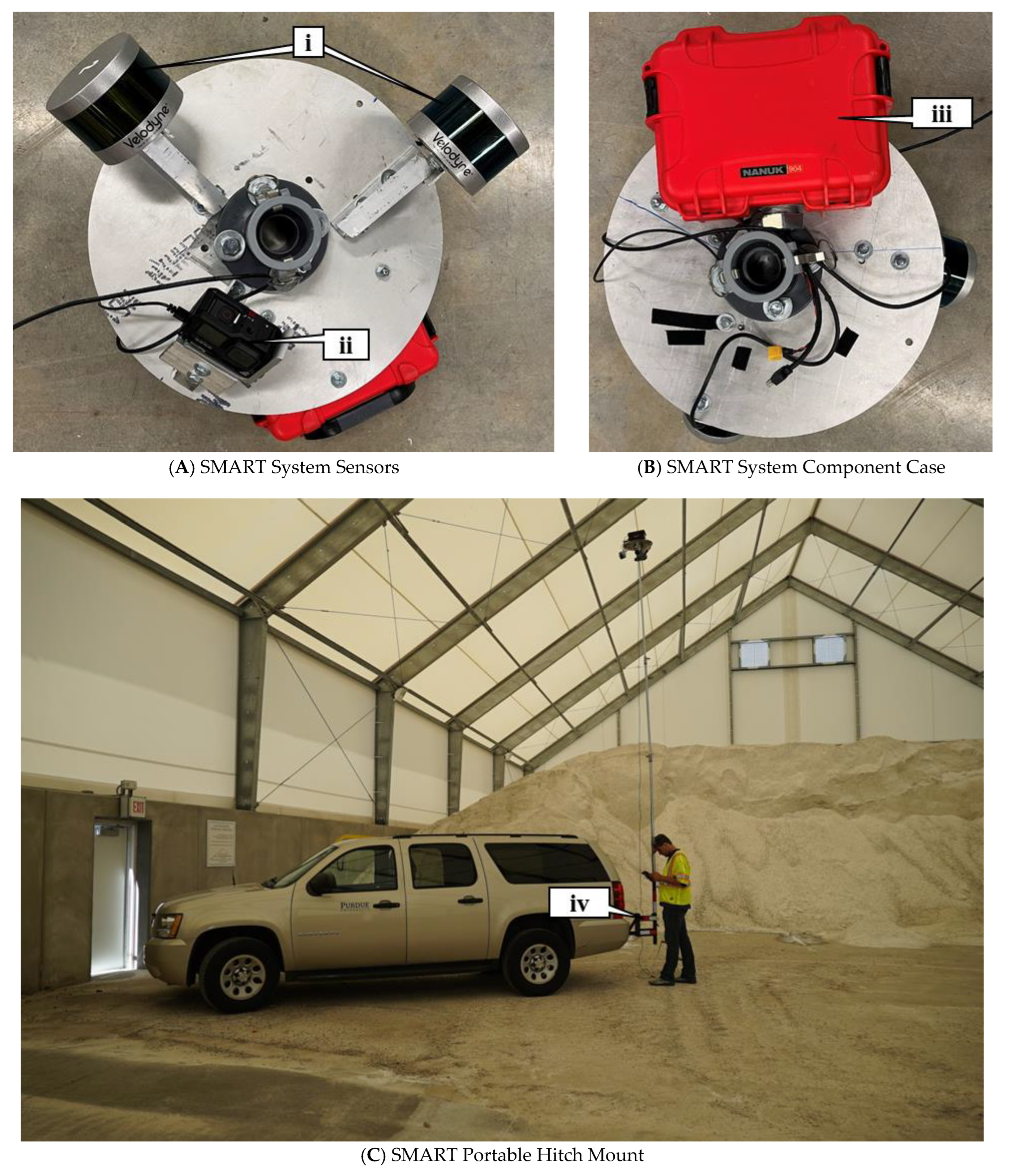
4. Data Collection Equipment
5. Overview of Methodology
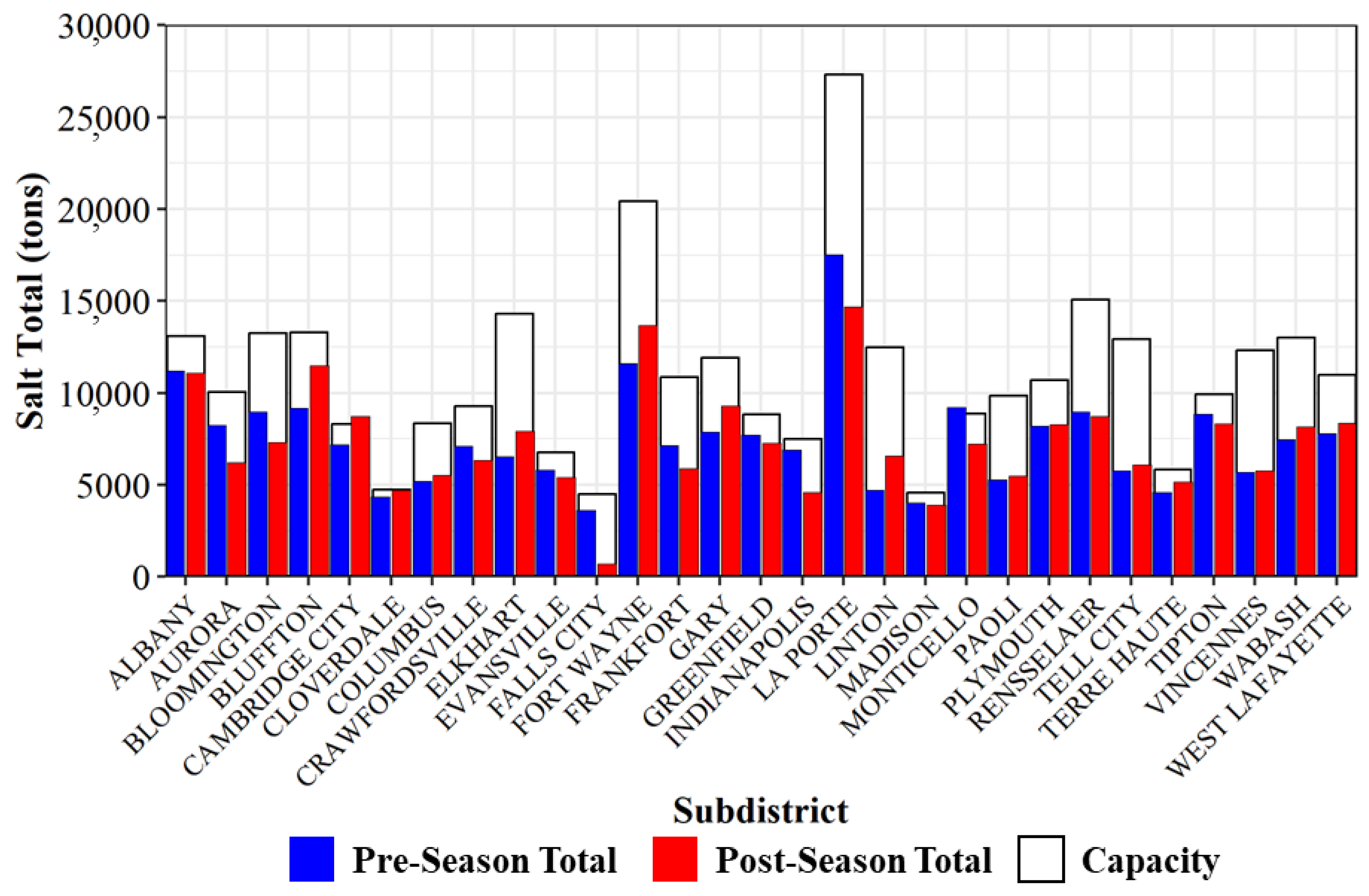
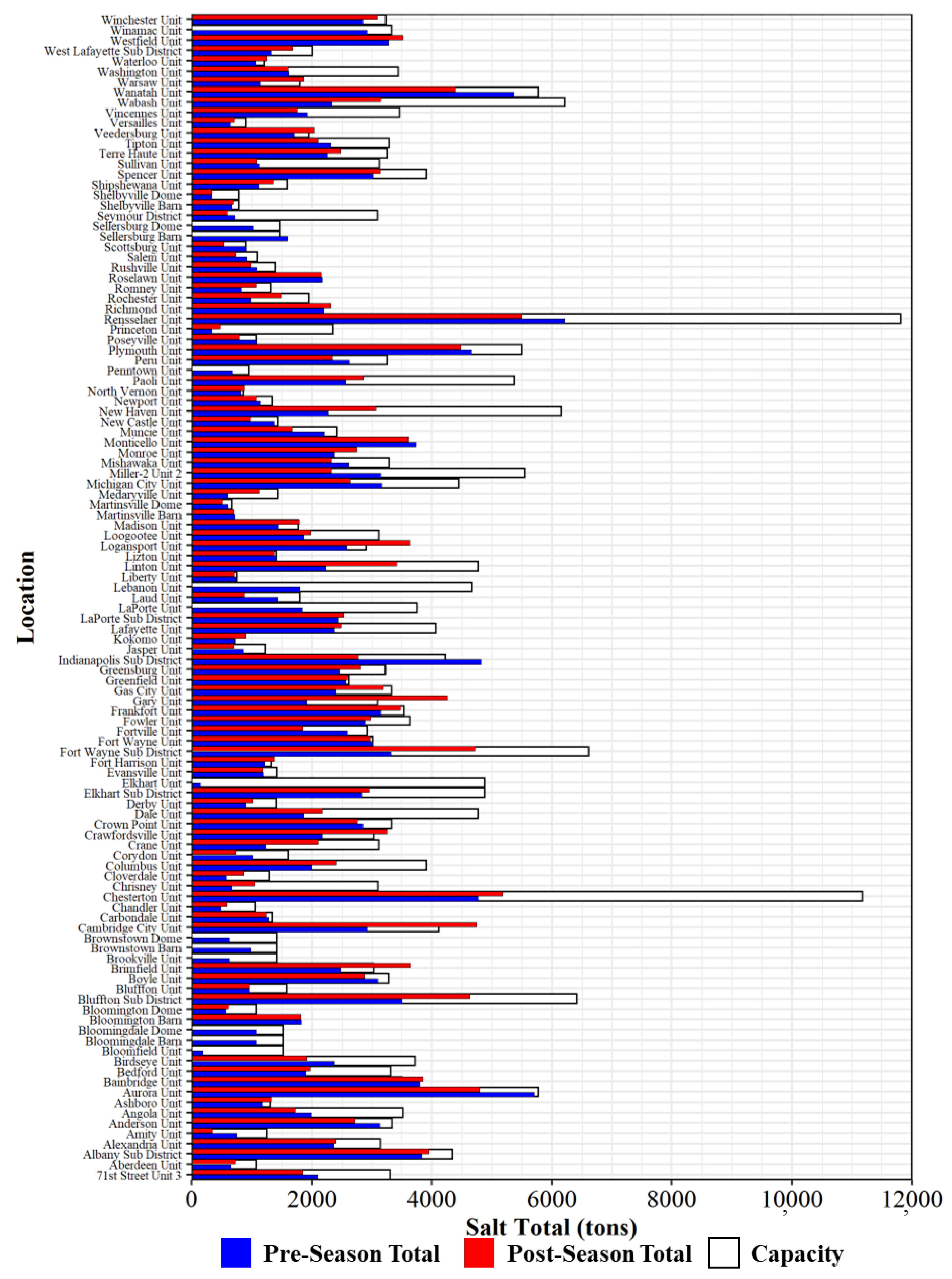
6. Statewide Inventory of 120 Facilities Using Portable Platform
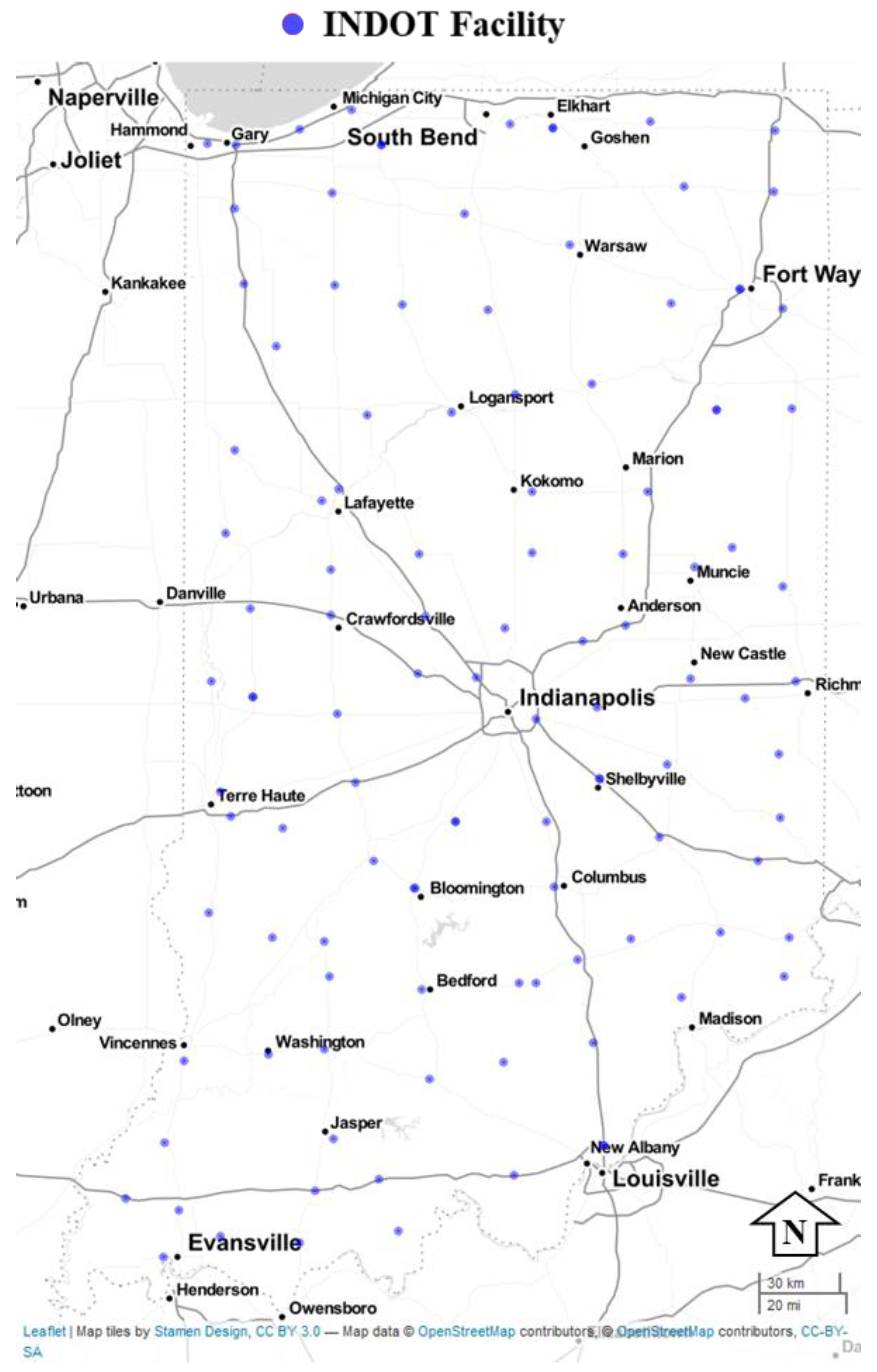
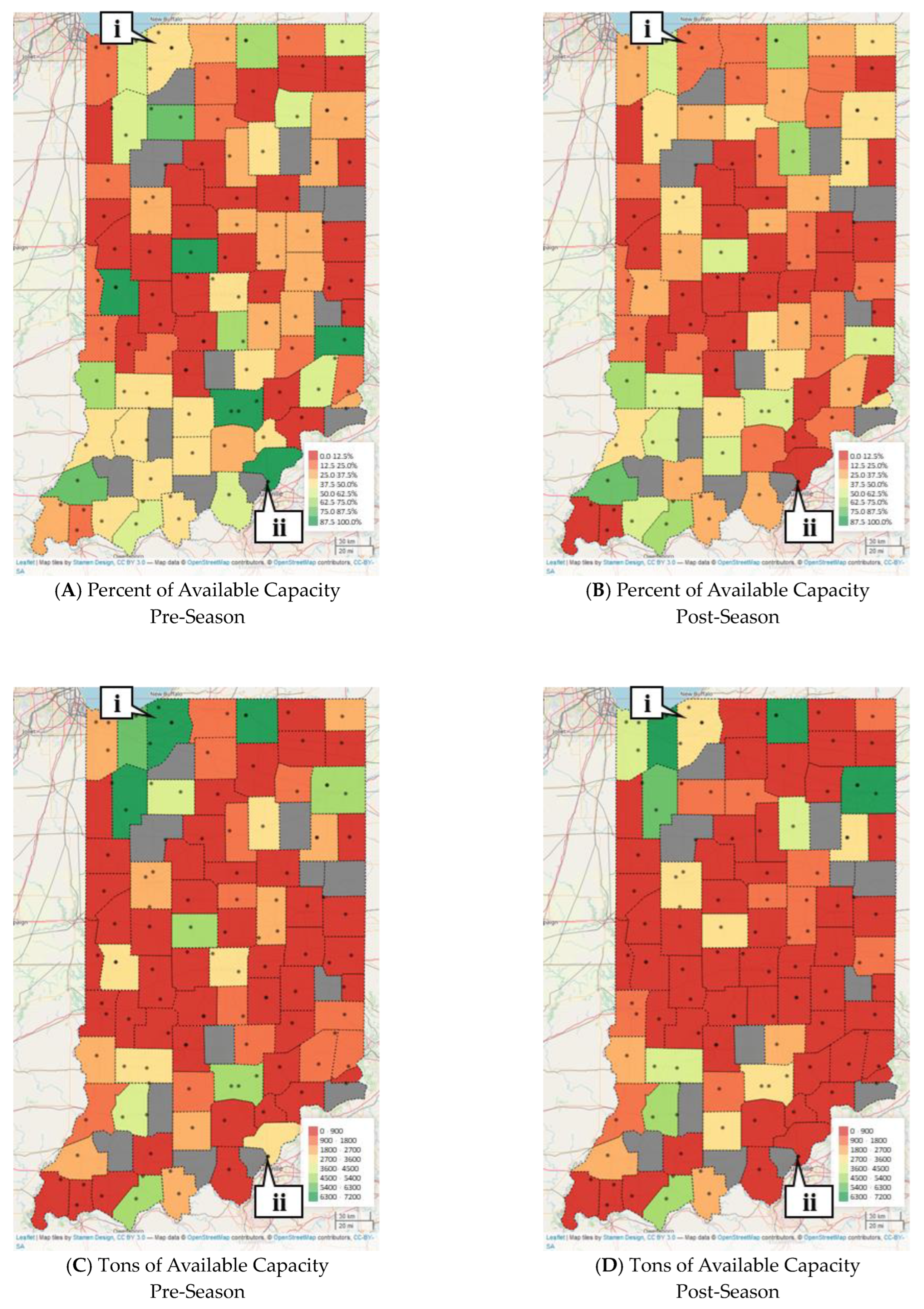
7. Geographic Mapping of County Salt Inventories
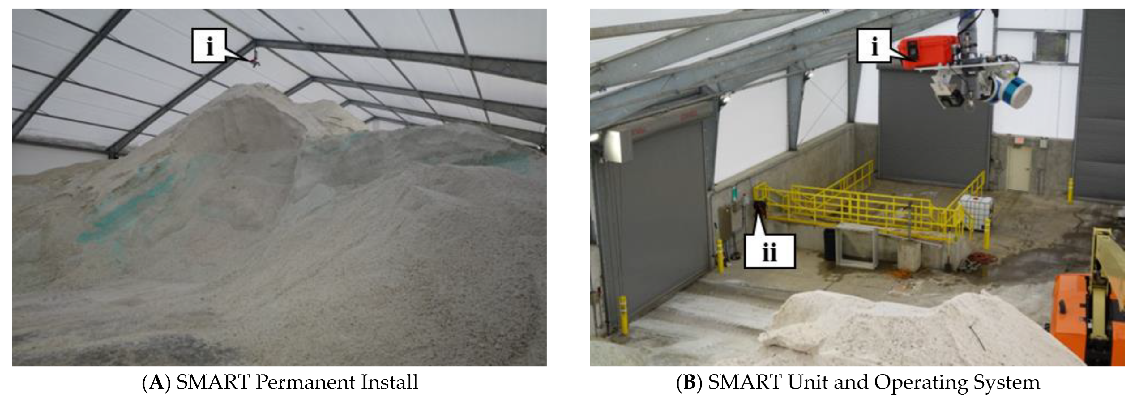
8. Fixed Salt Inventory Sensor Installations
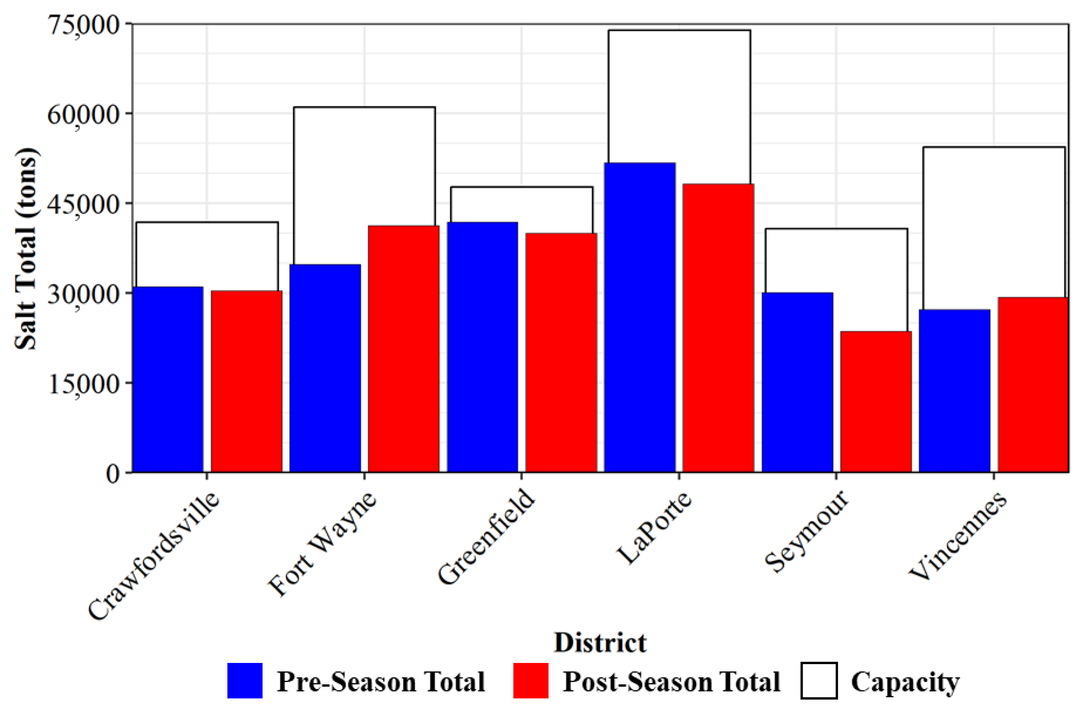
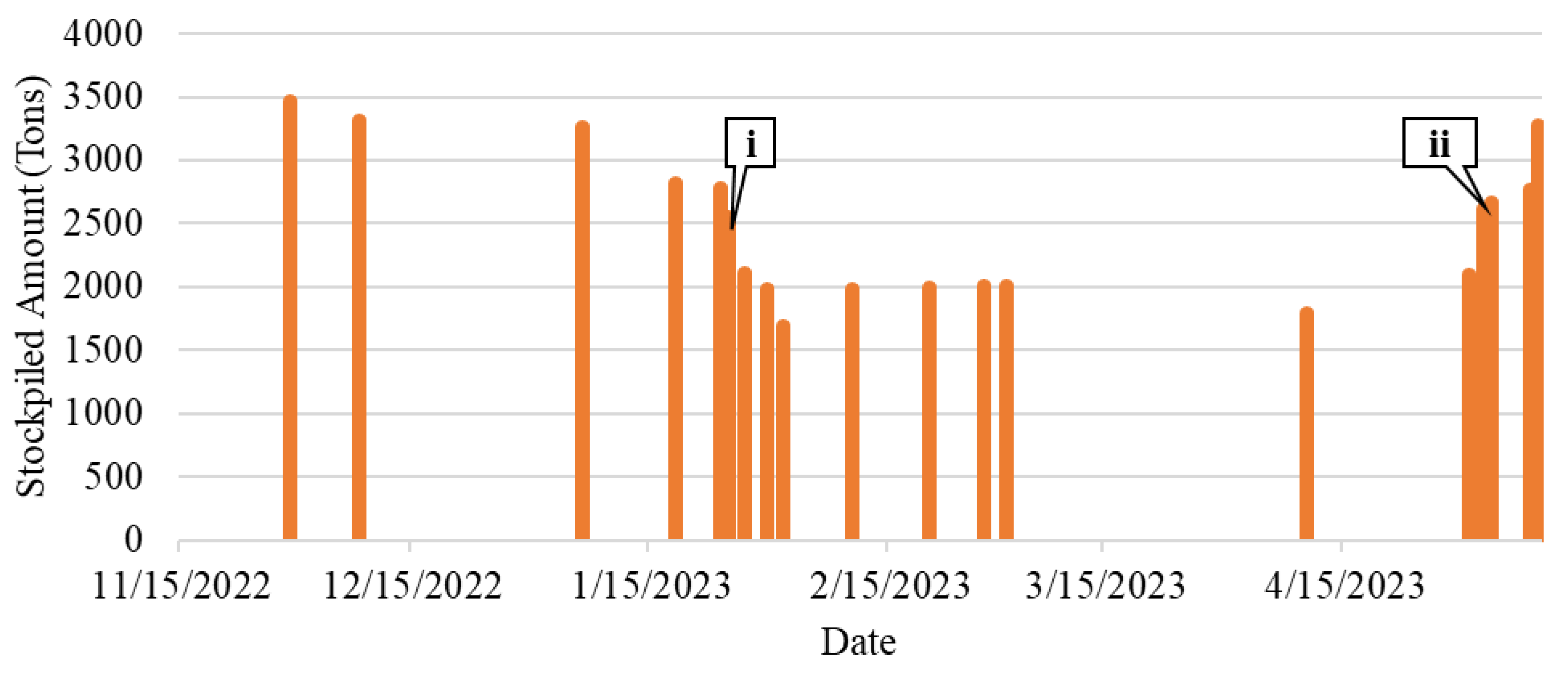
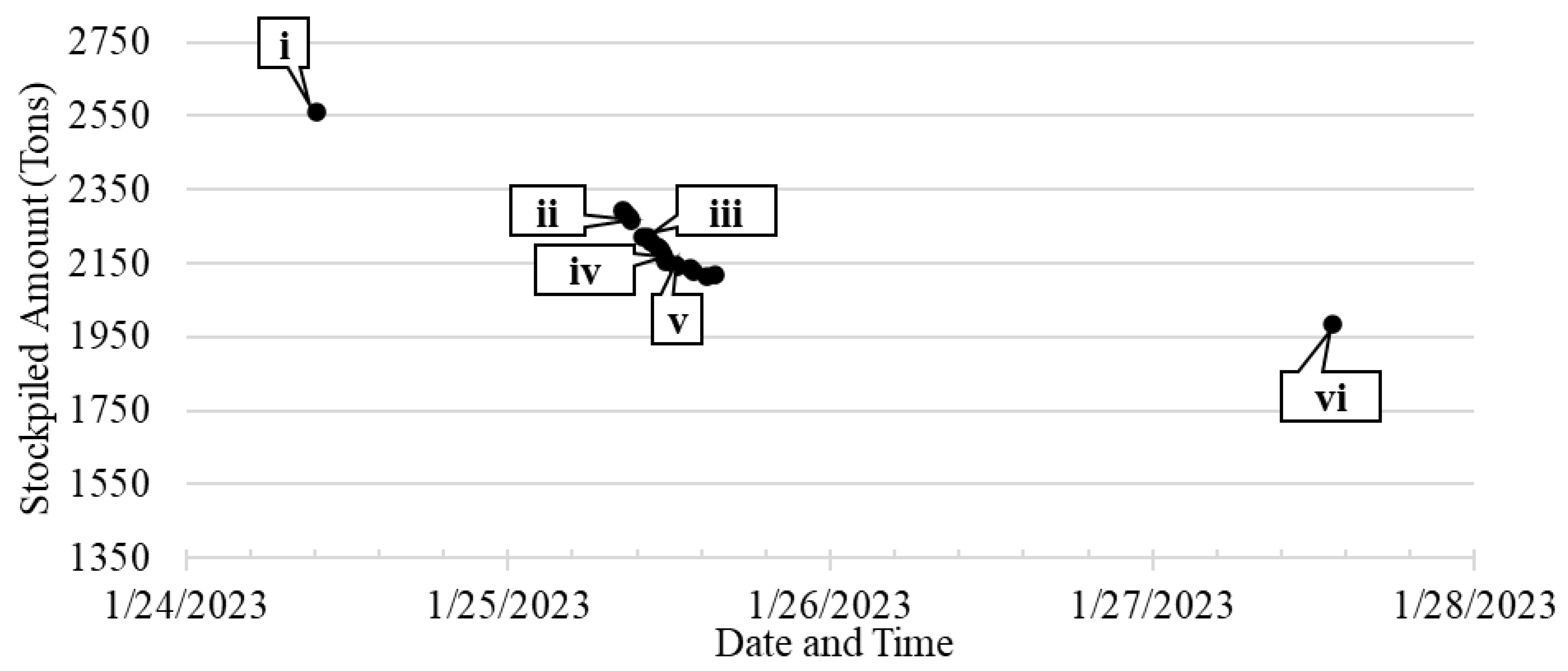
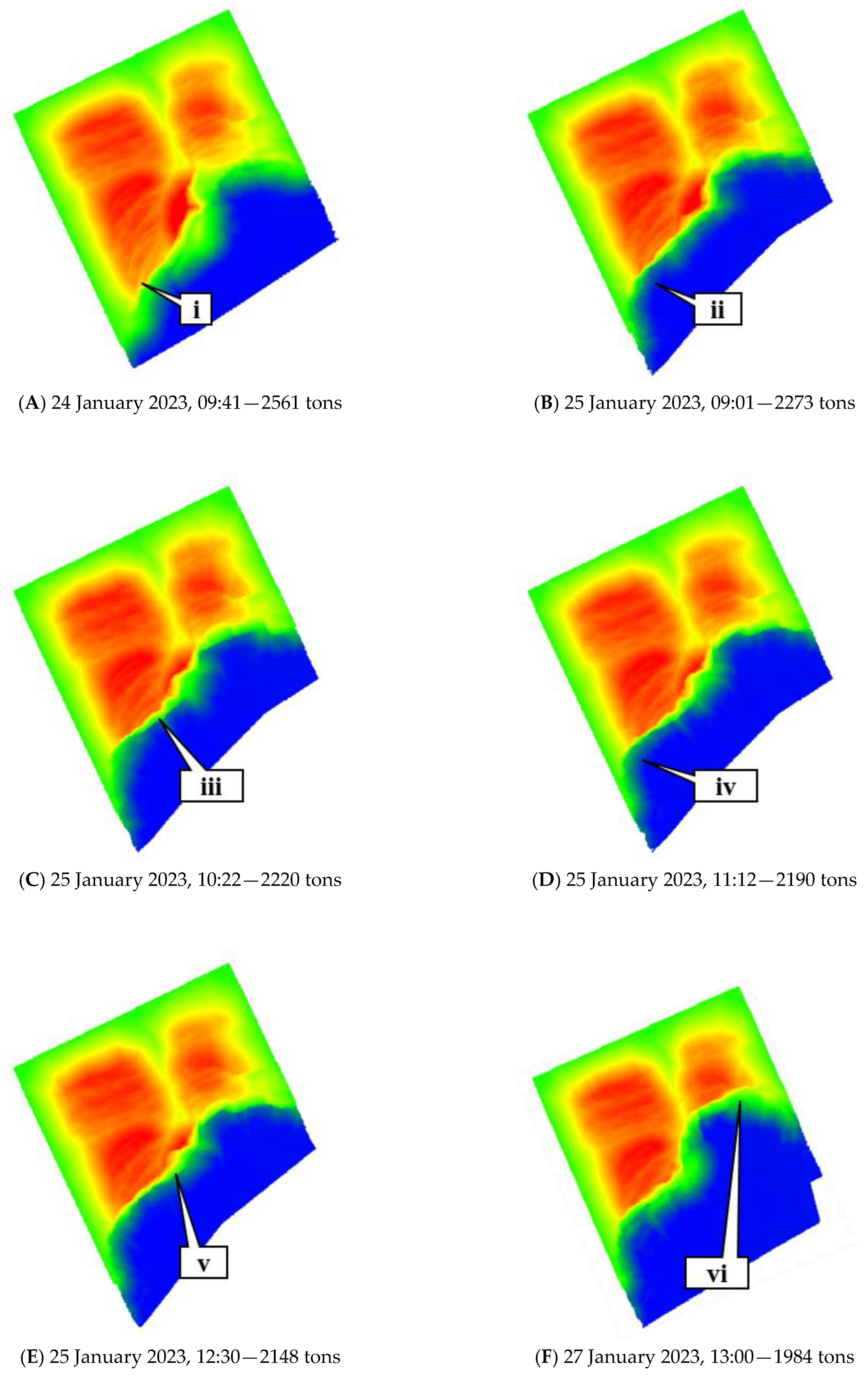
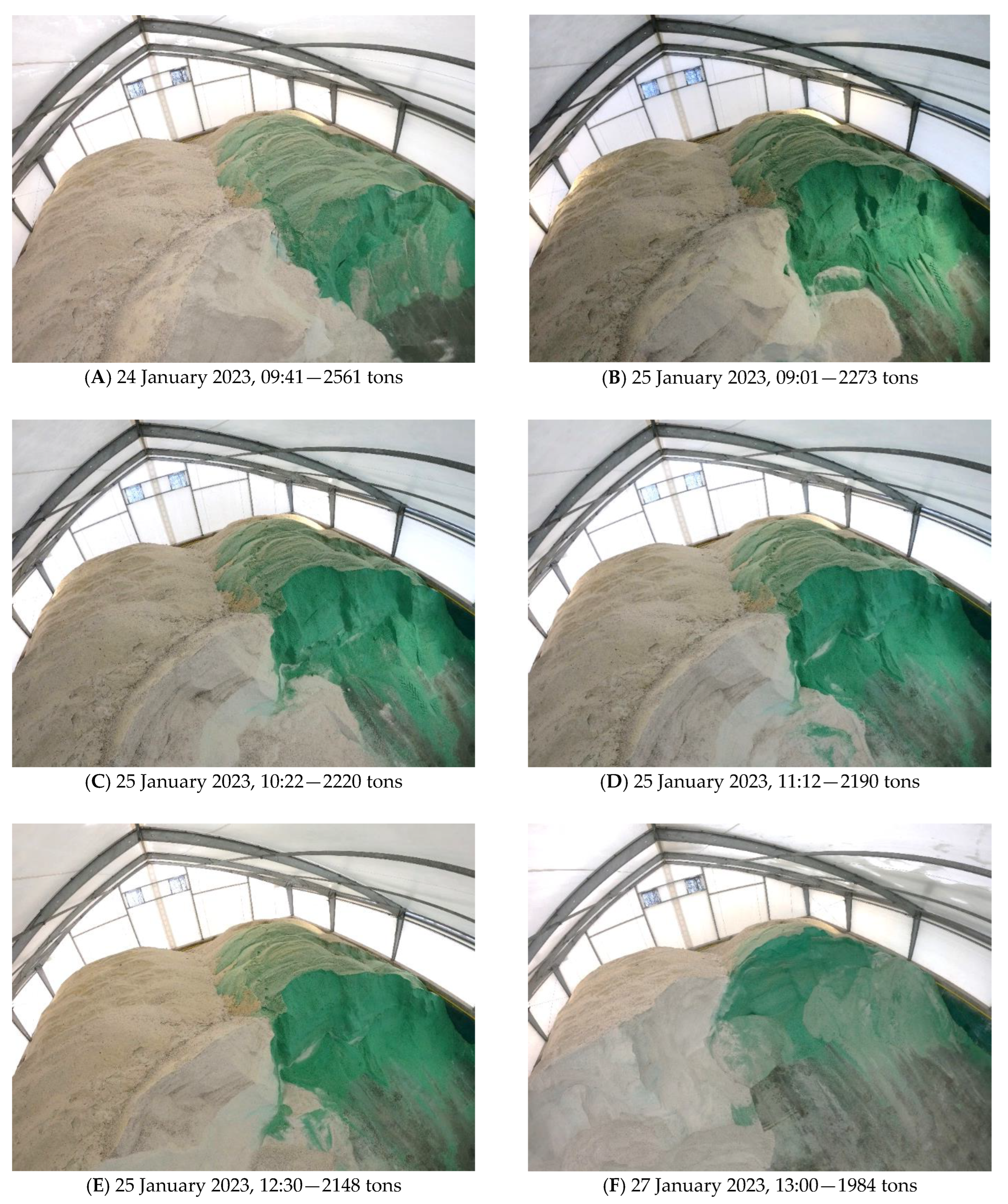
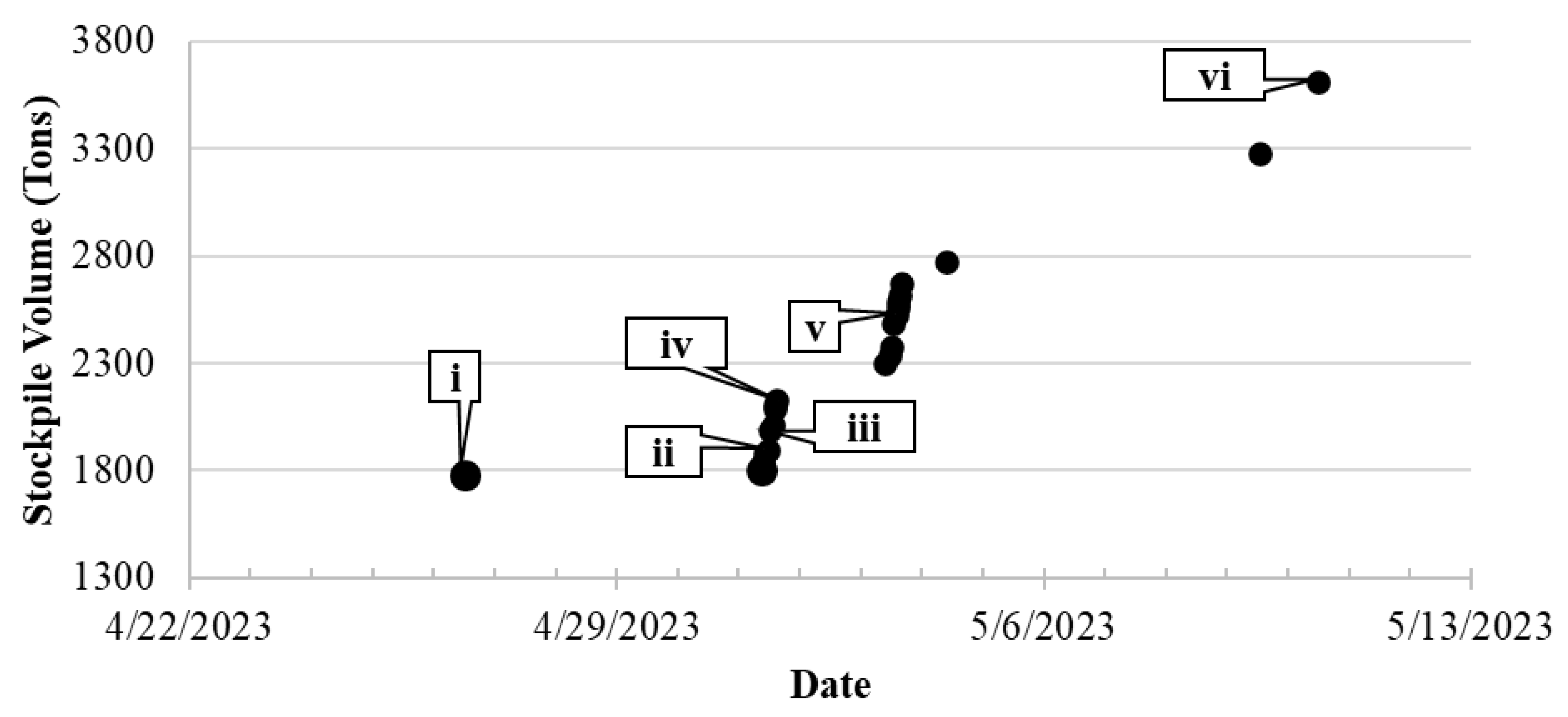
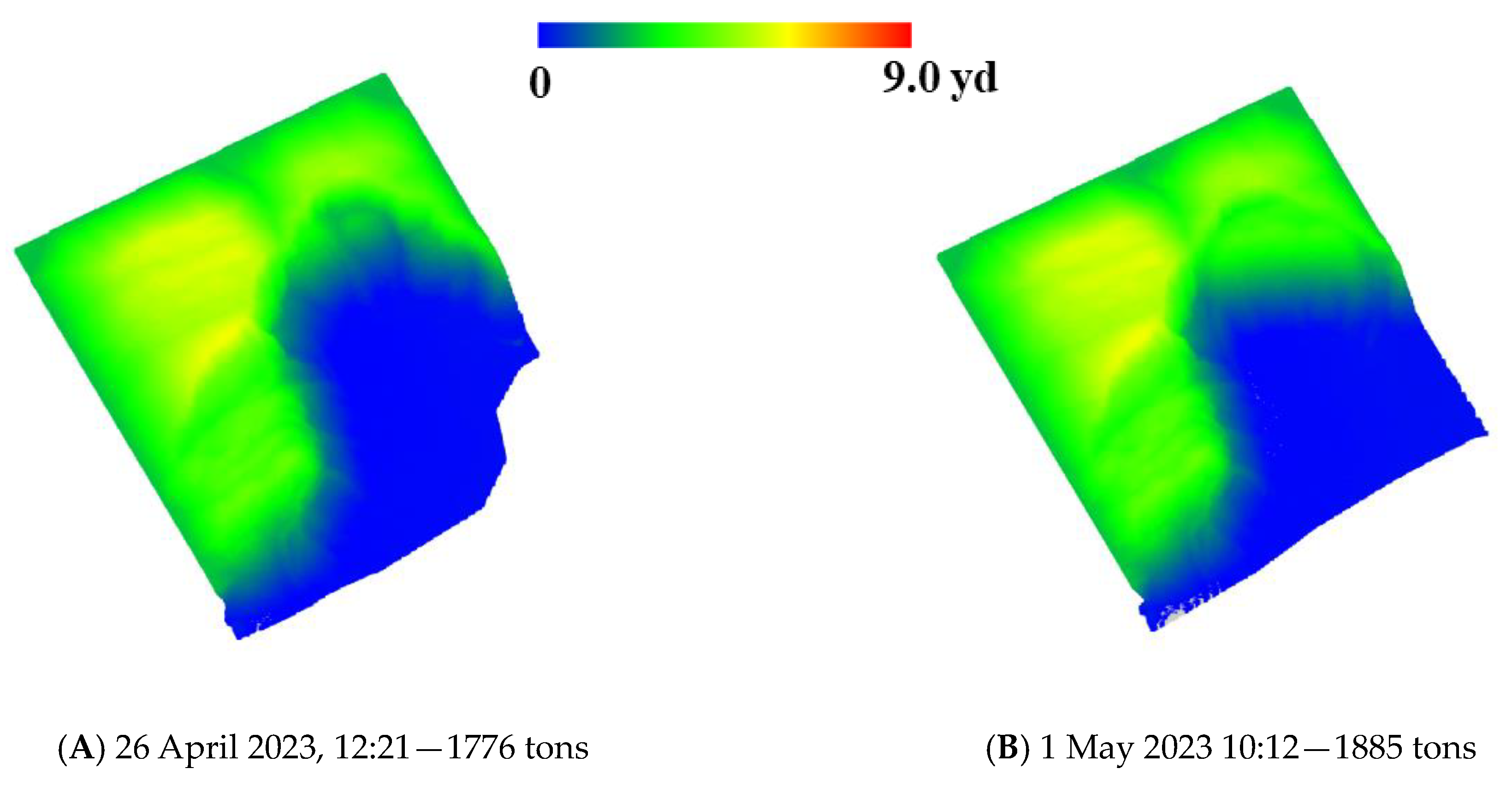
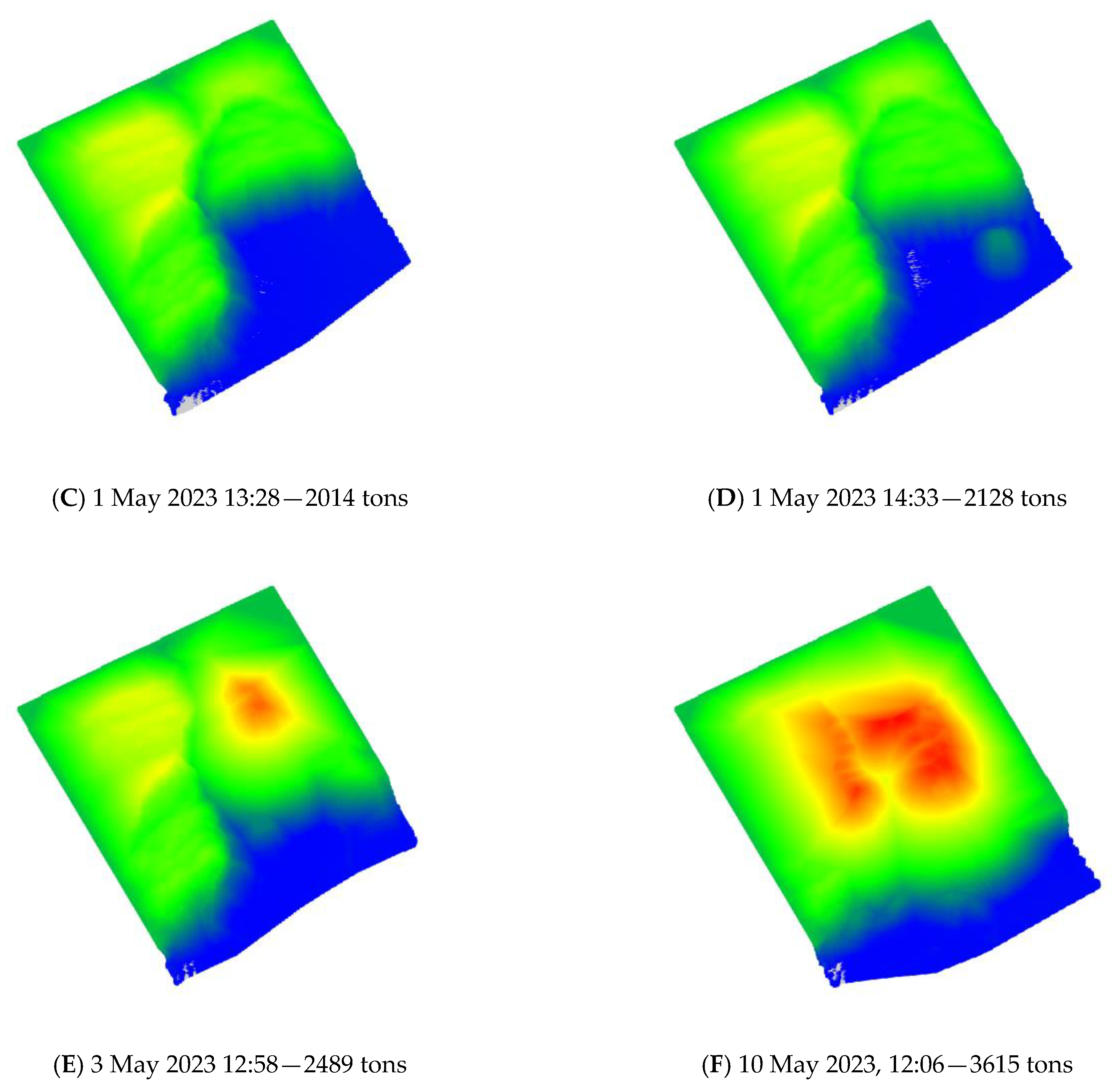
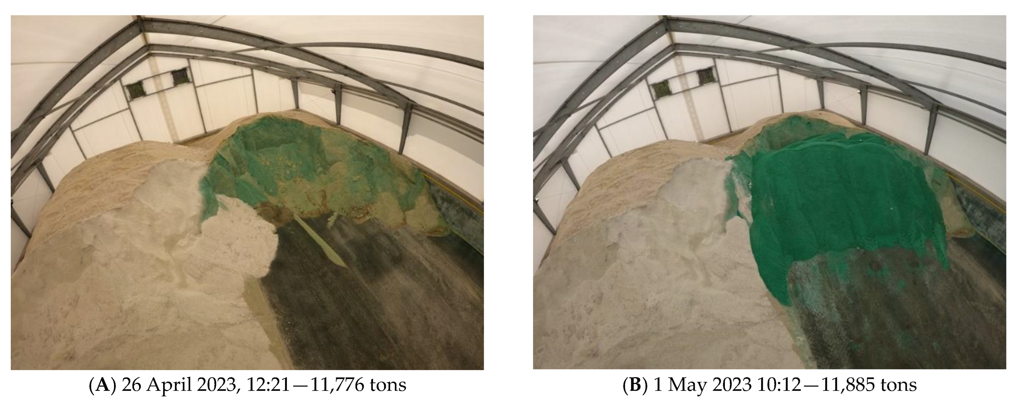
8.1. Winter Storm Usage Case Study
8.2. End of Sesaon Salt Replenishment Case Study
9. Evaluating Statewide Scalability
10. Conclusions and Future Scope
Author Contributions
Funding
Data Availability Statement
Conflicts of Interest
References
- Huang, H.; Tutumluer, E.; Luo, J.; Ding, K.; Qamhia, I.; Hart, J.M. Illinois Center for Transportation, and University of Illinois at Urbana-Champaign. Department of Civil and Environmental Engineering. In 3D Image Analysis Using Deep Learning for Size and Shape Characterization of Stockpile Riprap Aggregates—Phase 2; Publication FHWA-ICT-22-013; Illinois Department of Transportation: Springfield, IL, USA, 2022. [Google Scholar]
- Gago, R.M.; Pereira, M.Y.A.; Pereira, G.A.S. An Aerial Robotic System for Inventory of Stockpile Warehouses. Eng. Rep. 2021, 3, e12396. [Google Scholar] [CrossRef]
- Jiang, Y.; Huang, Y.; Liu, J.; Li, D.; Li, S.; Nie, W.; Chung, I.-H. Automatic Volume Calculation and Mapping of Construction and Demolition Debris Using Drones, Deep Learning, and GIS. Drones 2022, 6, 279. [Google Scholar] [CrossRef]
- Mahlberg, J.A.; Manish, R.; Koshan, Y.; Joseph, M.; Liu, J.; Wells, T.; McGuffey, J.; Habib, A.; Bullock, D.M. Salt Stockpile Inventory Management Using LiDAR Volumetric Measurements. Remote Sens. 2022, 14, 4802. [Google Scholar] [CrossRef]
- Luo, J.; Huang, H.; Ding, K.; Qamhia, I.I.A.; Tutumluer, E.; Hart, J.M.; Thompson, H.; Sussman, T.R. Toward Automated Field Ballast Condition Evaluation: Algorithm Development Using a Vision Transformer Framework. Transp. Res. Rec. 2023, 2677, 03611981231161350. [Google Scholar] [CrossRef]
- Qiu, Z.; Lin, D.; Lv, J.; Sun, Z.; Zheng, Z. A Closed Stockyard UAV Intelligent Inventory System. J. Phys. Conf. Ser. 2023, 2513, 012010. [Google Scholar] [CrossRef]
- Kasim, N.; Liwan, S.R.; Shamsuddin, A.; Zainal, R.; Kamaruddin, N.C. Improving On-Site Materials Tracking for Inventory Management in Construction Projects. In Proceedings of the International Conference of Technology Management, Business and Entrepreneurship, Malaka, Malaysia, 18–19 December 2012. [Google Scholar]
- Washington State Department of Labor & Industries. Worker Killed by Engulment in Salt Pile Fatality; Washington State Department of Labor & Industries: Tumwater, WA, USA, 2023. Available online: https://www.lni.wa.gov/safety-health/preventing-injuries-illnesses/hazardalerts/saltpileengulfmentjune10.pdf (accessed on 11 December 2023).
- Become a Drone Pilot|Federal Aviation Administration. Available online: https://www.faa.gov/uas/commercial_operators/become_a_drone_pilot (accessed on 25 July 2023).
- Kim, M. The Impact of Skill-Based Training across Different Levels of Autonomy for Drone Inspection Tasks. Master’s Thesis, Duke University, Durham, NC, USA, 2018. Available online: https://www.proquest.com/docview/2044069419/abstract/4D6FDE60F36245BBPQ/1 (accessed on 11 December 2023).
- Doroftei, D.; De Cubber, G.; De Smet, H. Reducing Drone Incidents by Incorporating Human Factors in the Drone and Drone Pilot Accreditation Process. In Advances in Human Factors in Robots, Drones and Unmanned Systems; Springer: Cham, Switzerland, 2021. [Google Scholar] [CrossRef]
- United States Environmental Protection Agency (EPA). National Pollutant Dsicharge Elimination System (NPDES) Multi-Sector General Permit (MSGP) for Stormwater Discharges Associated with Industrial Activity; United States Environmental Protection Agency (EPA): Washington, DC, USA, 2021.
- Salt and Stormwater Management|ISRI. Available online: https://www.isri.org/news-publications/news-details/2023/01/06/salt-and-stormwater-management (accessed on 5 December 2023).
- Wisconsin Department of Transportation. Salt Storage Needs Report 2021–2022; Wisconsin Department of Transportation: Milwaukee, WI, USA, 2023.
- Maryland Deparment of Transportation. Maryland Statewide Salt Management Plan; Maryland Deparment of Transportation: Hanover, MD, USA, 2012.
- How Do Weather Events Impact Roads?—FHWA Road Weather Management. Available online: https://ops.fhwa.dot.gov/weather/q1_roadimpact.htm (accessed on 21 July 2023).
- Snow & Ice–FHWA Road Weather Management. Available online: https://ops.fhwa.dot.gov/weather/weather_events/snow_ice.htm (accessed on 20 July 2023).
- Ciarallo, F.W.; Niranjan, S.; Brown, N. A Salt Inventory Management Strategy for Winter Maintenance. Oper. Supply Chain Manag. Int. J. 2015, 9, 31–49. [Google Scholar] [CrossRef]
- Nemati, A.; Sarim, M.; Hashemi, M.; Schnipke, E.; Reidling, S.; Jeffers, W.; Meiring, J.; Sampathkumar, P.; Kumar, M. Autonomous Navigation of UAV through GPS-Denied Indoor Environment with Obstacles; AIAA Infotech @ Aerospace: Kissimmee, FL, USA, 2015. [Google Scholar]
- Burdziakowski, P.; Bobkowska, K. UAV Photogrammetry under Poor Lighting Conditions—Accuracy Considerations. Sensors 2021, 21, 3531. [Google Scholar] [CrossRef] [PubMed]
- Manish, R.; Hasheminasab, S.M.; Liu, J.; Koshan, Y.; Mahlberg, J.A.; Lin, Y.-C.; Ravi, R.; Zhou, T.; McGuffey, J.; Wells, T.; et al. Image-Aided LiDAR Mapping Platform and Data Processing Strategy for Stockpile Volume Estimation. Remote. Sens. 2022, 14, 231. [Google Scholar] [CrossRef]
- Mora, O.E.; Chen, J.; Stoiber, P.; Koppanyi, Z.; Pluta, D.; Josenhans, R.; Okubo, M. Accuracy of Stockpile Estimates Using Low-Cost sUAS Photogrammetry. Int. J. Remote. Sens. 2020, 41, 4512–4529. [Google Scholar] [CrossRef]
- Winter Is Coming! And with It, Tons of Salt on Our Roads. United States Environmental Protection Agency. Available online: https://www.epa.gov/snep/winter-coming-and-it-tons-salt-our-roads (accessed on 11 December 2023).
- Mahlberg, J.A.; Desai, J.; Li, H.; Sakhare, R.S.; Wells, T.; Bullock, D.M. Calibration and Confidence in Snowplow Fleet Operations and Fleet Telematics. J. Transp. Technol. 2022, 12, 696–710. [Google Scholar] [CrossRef]
- Ravichandra Mouli, V. Using Automatic Vehicle Location (AVL) for Real-Time Maintenance Identification and Tracking. Master’s Thesis, Iowa State University, Ames, IA, USA, 2020. Available online: https://www.proquest.com/docview/2424137798/abstract/CE0F636F1F0441D5PQ/1 (accessed on 11 December 2023).
- Mahlberg, J.A.; Sakhare, R.S.; Li, H.; Mathew, J.K.; Bullock, D.M.; Surnilla, G.C. Prioritizing Roadway Pavement Marking Maintenance Using Lane Keep Assist Sensor Data. Sensors 2021, 21, 6014. [Google Scholar] [CrossRef] [PubMed]
- Velodyne Lidar Puck; Velodyne Lidar: San Jose, CA, USA; Available online: https://velodynelidar.com/wp-content/uploads/2019/12/63-9229_Rev-K_Puck-_Datasheet_Web.pdf (accessed on 11 December 2023).
- Puck Lidar Sensor, High-Value Surround Lidar; Velodyne Lidar: San Jose, CA, USA; Available online: https://velodynelidar.com/products/puck/ (accessed on 11 December 2023).
- GoPro Hero9 Black Review. Camera Decision. Available online: https://cameradecision.com/review/GoPro-Hero9-Black (accessed on 5 December 2023).
- Liu, J.; Hasheminasab, S.M.; Zhou, T.; Manish, R.; Habib, A. An Image-Aided Sparse Point Cloud Registration Strategy for Managing Stockpiles in Dome Storage Facilities. Remote. Sens. 2023, 15, 504. [Google Scholar] [CrossRef]
- Lin, Y.-C.; Liu, J.; Cheng, Y.-T.; Hasheminasab, S.M.; Wells, T.; Bullock, D.; Habib, A. Processing Strategy and Comparative Performance of Different Mobile LiDAR System Grades for Bridge Monitoring: A Case Study. Sensors 2021, 21, 7550. [Google Scholar] [CrossRef] [PubMed]
- Hovermap, S.T. Emesent. Available online: https://emesent.com/wp-content/uploads/2023/02/Hovermap-ST-Range-brochure.pdf (accessed on 5 December 2023).
- CloudCompare—Open Source Project. Available online: https://www.cloudcompare.org/ (accessed on 31 July 2023).


Disclaimer/Publisher’s Note: The statements, opinions and data contained in all publications are solely those of the individual author(s) and contributor(s) and not of MDPI and/or the editor(s). MDPI and/or the editor(s) disclaim responsibility for any injury to people or property resulting from any ideas, methods, instructions or products referred to in the content. |
© 2024 by the authors. Licensee MDPI, Basel, Switzerland. This article is an open access article distributed under the terms and conditions of the Creative Commons Attribution (CC BY) license (https://creativecommons.org/licenses/by/4.0/).
Share and Cite
Mahlberg, J.A.; Malackowski, H.; Joseph, M.; Koshan, Y.; Manish, R.; DeLoach, Z.; Habib, A.; Bullock, D.M. Statewide Implementation of Salt Stockpile Inventory Using LiDAR Measurements: Case Study. Remote Sens. 2024, 16, 410. https://doi.org/10.3390/rs16020410
Mahlberg JA, Malackowski H, Joseph M, Koshan Y, Manish R, DeLoach Z, Habib A, Bullock DM. Statewide Implementation of Salt Stockpile Inventory Using LiDAR Measurements: Case Study. Remote Sensing. 2024; 16(2):410. https://doi.org/10.3390/rs16020410
Chicago/Turabian StyleMahlberg, Justin Anthony, Haydn Malackowski, Mina Joseph, Yerassyl Koshan, Raja Manish, Zach DeLoach, Ayman Habib, and Darcy M. Bullock. 2024. "Statewide Implementation of Salt Stockpile Inventory Using LiDAR Measurements: Case Study" Remote Sensing 16, no. 2: 410. https://doi.org/10.3390/rs16020410