
A Framework for Fine-Grained Land-Cover Classification Using 10 m Sentinel-2 Images

1
School of Surveying and Land Information Engineering, Henan Polytechnic University, Jiaozuo 454000, China
2
State Key Laboratory of Remote Sensing Science, Aerospace Information Research Institute, Chinese Academy of Sciences, Beijing 100094, China
3
China Remote Sensing Satellite Ground Station, Aerospace Information Research Institute, Chinese Academy of Sciences, Beijing 100094, China
*
Author to whom correspondence should be addressed.
Remote Sens. 2024, 16(2), 390; https://doi.org/10.3390/rs16020390
Submission received: 23 November 2023
/
Revised: 9 January 2024
/
Accepted: 12 January 2024
/
Published: 18 January 2024
(This article belongs to the Special Issue Deep Learning for Spectral-Spatial Hyperspectral Image Classification)
Abstract
:Land-cover mapping plays a crucial role in resource detection, ecological environmental protection, and sustainable development planning. The existing large-scale land-cover products with coarse spatial resolution have a wide range of categories, but they suffer from low mapping accuracy. Conversely, land-cover products with fine spatial resolution tend to lack diversity in the types of land cover they encompass. Currently, there is a lack of large-scale land-cover products simultaneously possessing fine-grained classifications and high accuracy. Therefore, we propose a mapping framework for fine-grained land-cover classification. Firstly, we propose an iterative method for developing fine-grained classification systems, establishing a classification system suitable for Sentinel-2 data based on the target area. This system comprises 23 fine-grained land-cover types and achieves the most stable mapping results. Secondly, to address the challenges in large-scale scenes, such as varying scales of target features, imbalanced sample quantities, and the weak connectivity of slender features, we propose an improved network based on Swin-UNet. This network incorporates a pyramid pooling module and a weighted combination loss function based on class balance. Additionally, we independently trained models for roads and water. Guided by the natural spatial relationships, we used a voting algorithm to integrate predictions from these independent models with the full classification model. Based on this framework, we created the 2017 Beijing–Tianjin–Hebei regional fine-grained land-cover product JJJLC-10. Through validation using 4254 sample datasets, the results indicate that JJJLC-10 achieves an overall accuracy of 80.3% in the I-level validation system (covering seven land-cover types) and 72.2% in the II-level validation system (covering 23 land-cover types), with kappa coefficients of 0.7602 and 0.706, respectively. In comparison with widely used land-cover products, JJJLC-10 excels in accurately depicting the spatial distribution of various land-cover types and exhibits significant advantages in terms of classification quantity and accuracy.
1. Introduction
Land cover reflects essential information about the Earth’s surface characteristics and is one of the critical variables for monitoring the Sustainable Development Goals (SDGs). It holds great significance for research in natural resource management, ecological environmental protection, and urban planning [1,2,3]. With the rapid development of the economy and society, issues such as soil degradation, environmental pollution, and urban expansion have shown a noticeable upward trend. Therefore, there is an urgent need for accurate and detailed land-cover information to provide a scientific basis for policy formulation and sustainable development research.
At present, high-resolution fine-scale land-cover products covering large areas are limited. Over recent decades, the spatial resolution and quality of global or regional land-cover products have gradually evolved from coarse to fine. Land-cover products based on coarse resolution data, such as AVHRR and MODIS [4,5,6,7,8], are commonly recognized by users as possessing a lack of spatial detail, low classification accuracy, and poor consistency between different products, making them inadequate for modern applications [9,10]. The high-resolution remote sensing data freely available from Landsat and Sentinel-2 provide data support for producing more fine-grained land-cover products. For instance, Gong et al. [11] generated the 2015 global 30 m land-cover product FROM_GLC30 based on Landsat data, which includes 28 land-cover types, but the overall accuracy was only 52.76%. Zhang et al. [12] produced the 2015 global 30 m land-cover product GLC_FCS30 by combining the multi-temporal random forest model, time series of Landsat imagery, and global training data. It contains 16 global land-cover types and 14 regional fine-grained land-cover types, with overall accuracy rates of 71.4% and 68.7%, respectively. However, due to the low classification accuracy of fine-grained land-cover types, it is difficult to capture the spatial detail information of the land cover, hindering the fine-scale application of existing products. With the rapid enhancement of data storage and computing power, it becomes feasible to produce land-cover products with finer resolution [13,14], such as FROM_GLC10 [15], ESA World Cover [16], and ESRI Land Cover [17], which can support the fine-grained monitoring of global land cover and its changes. In general, the existing large-scale, coarse-resolution products offer a wide range of categories, but suffer from low mapping accuracy. On the other hand, for high-resolution products, due to limitations in classification systems and algorithms, the improvement in data quality does not yield more fine-grained classification quantity.
Establishing a scientific classification system is important in achieving fine-grained land-cover classification. In 1996, the Food and Agriculture Organization of the United Nations (FAO) [18] established a standard and comprehensive land-cover classification system—LCCS (Land Cover Classification System), which is suitable for research at various scales and with different data sources. Some classification systems, such as the European Union Joint Research Center GLC2000 [6] and the Basic Geographic National Conditions Monitoring Classification Standard (CH/T 9029-2019) [19], drew upon the design concepts of the LCCS classification system. However, these classification systems exhibit significant differences in terms of compatibility across different scenarios, often necessitating additional data processing and conversion for their use [20]. Subsequently, in 2010, China initiated essential research on global land-cover remote sensing mapping techniques [21]. Chen et al. [22] utilized the pixel object knowledge method to divide the world into ten types, and this classification system is currently one of the most widely applied systems globally and at regional levels. Nevertheless, these predefined categories are challenging in terms of encompassing all of the natural land-cover types. Regarding land-cover product mapping, it is advisable to explore the finest possible category system based on the data and target scenarios, ultimately leading to superior land-cover products.
The classification method employed is the critical factor influencing the accuracy of large-scale land-cover mapping. As exemplified by convolutional neural networks (CNNs), deep learning approaches exhibit strong feature extraction capabilities and are widely used in large-scale land-cover mapping tasks [23,24,25,26]. However, due to the significant scale variations and diverse shapes of different land features, the conventional layers used in the above research have the problem of a limited receptive field, hindering the comprehensive learning of contextual information [27,28]. The limitation results in slight patch effects at the transition zones of features with similar characteristics, leading to the discontinuity of some slender land features in the classification results, thereby impeding the practical application of land-cover products. While transformers utilize multi-head self-attention modules to rapidly capture long-range feature relationships, thereby maximizing the utilization of global context information, they provide innovative concepts for large-scale land-cover mapping [29,30]. Liu et al. [31] proposed the Swin Transformer in 2021, which uses sliding windows and hierarchical structures to extract multi-scale features. Based on the idea of Swin-T, Cao et al. [32] proposed Swin-UNet in 2021, which is a U-shaped encoding–decoding architecture of the base transformer and has achieved great success in the field of medical image segmentation. In addition, due to the issue of imbalanced sample sizes in the training sample data [33], models tend to favor learning the majority class during training while ignoring rare categories, thus affecting the overall classification accuracy [34]. Existing research has attempted to rebalance sample quantities through re-sampling and re-weighting [35]. However, these methods have specific shortcomings in specific use cases, such as the fact that under-sampling can lead to the loss of essential feature information, while over-sampling can result in overfitting for minority class data [36]. When dealing with multi-classification tasks, the re-weighting method increases the complexity of determining the appropriate weight for each category due to the potential correlation between different categories [37].
In general, the limitations of classification systems and classification algorithms restrict the production of fine-grained land-cover products for large-scale scenarios. We propose a mapping framework for fine-grained land-cover classification, and its main contributions are as follows:
- This paper proposes a fine-grained classification system iteration algorithm, which aims to explore a stable classification system tailored to specific sensors based on the target region. We applied this method to deduce a classification system for Sentinel-2 data, initially training the model with the sample dataset and constructing the initial classification system. Subsequently, the trained model was used to predict the target region, merging land-cover types with insufficient discriminability at a 10 m resolution. Through multiple iterations and the refinement of the classification system, we ultimately developed a stable classification system encompassing 23 land-cover types and achieved optimal mapping results.
- The paper aims to address challenges in large-scale scenes, such as varying scales of target features, imbalanced sample quantities, and weak connectivity of slender features. We introduce a pyramid pooling module based on Swin-UNet to enhance the model’s perception of features at different scales. Additionally, we designed a combination loss function based on class balance, balancing the model’s learning ability for different features. Independent model training was conducted for roads and water. Leveraging spatial relationships in natural features as clues, we used a voting algorithm to integrate predictions from independent models and the overall classification model, enhancing the generalization ability of slender features in complex scenarios.
- Based on this framework, we produced the 2017 fine-grained land-cover product JJJLC-10 for the Beijing–Tianjin–Hebei region. We quantitatively assessed the accuracy of JJJLC-10 using a validation sample set of 4254 samples and visually compare it with four mainstream large-scale land-cover products, thus demonstrating the advantages of our product more intuitively. To the best of our knowledge, it is by far the richest product in terms of surface coverage types at the 10 m scale.
2. Materials
2.1. Study Area
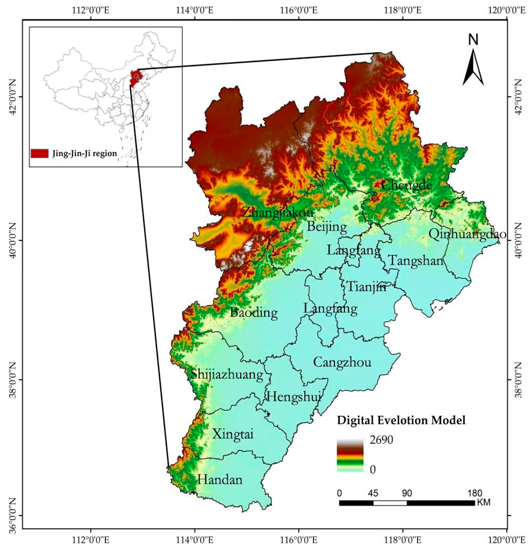
The Beijing–Tianjin–Hebei region is located in northeastern China, ranging from latitudes 36° to 42°N and longitudes 113° to 119°E. The region is bordered by the Bohai Sea in the east, the Taihang Mountains in the west, the North China Plain in the south, and the Yanshan Mountains in the north, as shown in Figure 1. The terrain in this area is complex and diverse, with the northwestern part of the region dominated mainly by mountains, hills, and plateaus and the southeastern part dominated by plains with an overall stepped downward trend of high in the northwestern part of the region and low in the southeast part of the region. The Beijing–Tianjin–Hebei region covers a total area of about 218,600 square kilometers, mainly including Beijing, Tianjin, and 11 cities in Hebei Province, accounting for 2.27% of the total land area. As of the end of 2022, the permanent population of the Beijing–Tianjin–Hebei region exceeded 130 million people, and the GDP exceeded CNY 10 trillion, accounting for 8.3% of the total national GDP, which has positively promoted the country’s economic development.
2.2. Data and Preprocessing
2.2.1. Remote Sensing Data
The Sentinel-2 satellite is a multispectral Earth observation satellite launched by the European Space Agency’s Copernicus program. It consists of two satellites, Sentinel-2A and Sentinel-2B, which operate alternately with a five-day revisit period. The multispectral imager carried by the satellite covers 13 spectral bands with spatial resolutions of 10 m, 20 m, and 60 m. The specific spectral parameters are shown in Table 1. The Sentinel-2 data boast a remarkable spatial resolution of 10 m, allowing for the clear capture of intricate surface details. Moreover, the utilization of 13 spectral bands offers a wealth of spectral information crucial for precise land-cover classification, enabling the identification and differentiation of various land-cover types. The combination of a short data return period and open access further establishes a reliable and timely database for in-depth studies on land cover and its dynamic changes. Since its launch in 2015, data from Sentinel-2 have been widely employed by researchers in the exploration of land-cover classification and change detection, yielding noteworthy results [38]. Therefore, in this paper, all of the spectral band information from Sentinel-2 data is used for refined land-cover mapping in the Beijing–Tianjin–Hebei region. According to the standard of less than 5% cloudiness, a total of 110 scenes of Level-1C data from May to September were downloaded from the ESA website (https://scihub.copernicus.eu/, accessed on 17 December 2022).
The GF-1 satellite, China’s first high-resolution Earth observation satellite, launched on 26 April 2013. It carries a high-resolution camera (PMS) that includes a panchromatic band with a spatial resolution of 2 m and four multispectral bands with spatial resolutions of 8 m. These multispectral bands consist of red, green, blue, and near-infrared bands. We used GF-1 data for labeling and data from the Land Observation Satellite Data Service Platform of the China Center for Resources Satellite Data and Application (https://data.cresda.cn/, accessed on 12 February 2023). The time range is generally consistent with Sentinel-2 data.
2.2.2. Data Processing
Due to the downloaded Sentinel-2 data being Level-1C atmospheric reflectance products, we applied the Sen2Cor plugin to perform atmospheric correction on the Level-1C data, obtaining Level-2A data. Additionally, we utilized SNAP 9.0 software developed by the European Space Agency for preprocessing Sentinel data, uniformly re-sampling the resolution of the 13 bands to 10 m. Subsequently, we cropped the remote sensing images based on the administrative boundaries of the study area.
GF-1 data are susceptible to weather conditions, making it necessary to perform radiometric enhancement on the decompressed panchromatic and multispectral files. This enhancement renders the ground features in the image more distinct and prominent, facilitating visual interpretation. Then, the orthorectification of the radiometrically calibrated image is carried out based on the Image Rational Polynomial Coefficient (RPC) file and the Digital Elevation Model (DEM), effectively mitigating geometric distortions. Finally, a panchromatic fusion method is applied to merge the panchromatic and multispectral bands, resulting in an image with a spatial resolution of 2 m.
2.3. Sample
Adequate and accurate training samples are essential for large-scale land-cover classification. Currently, the training sample collection methods mainly include manual visual interpretation of samples and the automatic extraction of training samples from existing land-cover products [12], approaches widely used in large-scale land-cover classification. However, due to the coarse spatial resolution of existing land-cover products and the lack of diversity in the included land-cover types, the training samples obtained from them lack fine-grained land-cover information, making it challenging to meet the research requirements for fine land-cover classification. Therefore, creating a labeled dataset with fine-grained land-cover types is essential.
The granularity of resolution affects the fineness of feature identification and the number of categories. GF-1 imaging provides detailed spatial and spectral information, enabling the clear capture of richer and more fine-grained land-cover features, making it suitable for creating fine land-cover label datasets. The fine land-cover label datasets utilized in this study were meticulously curated through the collaborative efforts of over ten team members. First, based on the geographic location and topographical characteristics of the Beijing–Tianjin–Hebei region, approximately 39% of the study area was selected as the interpretation area. Referring to the existing medium and high-resolution land-cover products and the results of the dynamic monitoring of geographical conditions, our team visually interpreted and pixel-level labeled various land-cover types in the interpretation sample area using high-resolution remote sensing images. The category was refined to the three levels of geographical conditions, encompassing a comprehensive set of 91 distinct land-cover types. To ensure the precision of the labeled datasets, any contentious types were addressed through on-site field visits, where ground objects of debate were marked and resolved. Simultaneously, we employed the Nearest Neighbor Interpolation method to resample the labeled data to a 10 m resolution, resulting in the creation of 15 image and label datasets sized 16,053 × 16,053 pixels in the study area. These datasets cover 39% of the Beijing–Tianjin–Hebei region, spanning an area of 85,300 square kilometers.
Due to the GPU’s capacity limitation, loading the entire remote sensing images and labels into the GPU for training is unfeasible. Therefore, to meet the model input requirements, this paper employed the sliding window clipping method to segment images and labels of size 16,053 × 16,053 into 512 × 512. This process yielded a total of 15,411 standardized slices, each measuring 512 × 512 pixels. According to the ratio of 8:2, a total of 12,328 training samples and 3082 testing samples of size 512 × 512 were obtained from the standardized slices for model training and accuracy validation, respectively.
To improve the convergence speed and stability of the model during training, we normalized each band of the Sentinel-2 image across the entire training sample before commencing the training process. The normalization principle is as follows:
where represents the normalized image data, represents the original input image data, and and represent the mean and standard deviation of each band in the Sentinel-2 data.
3. Methods
3.1. Overall Framework
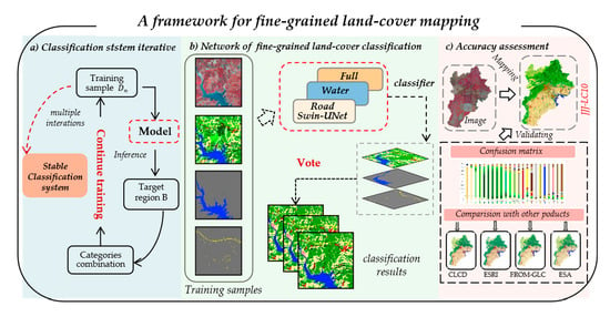
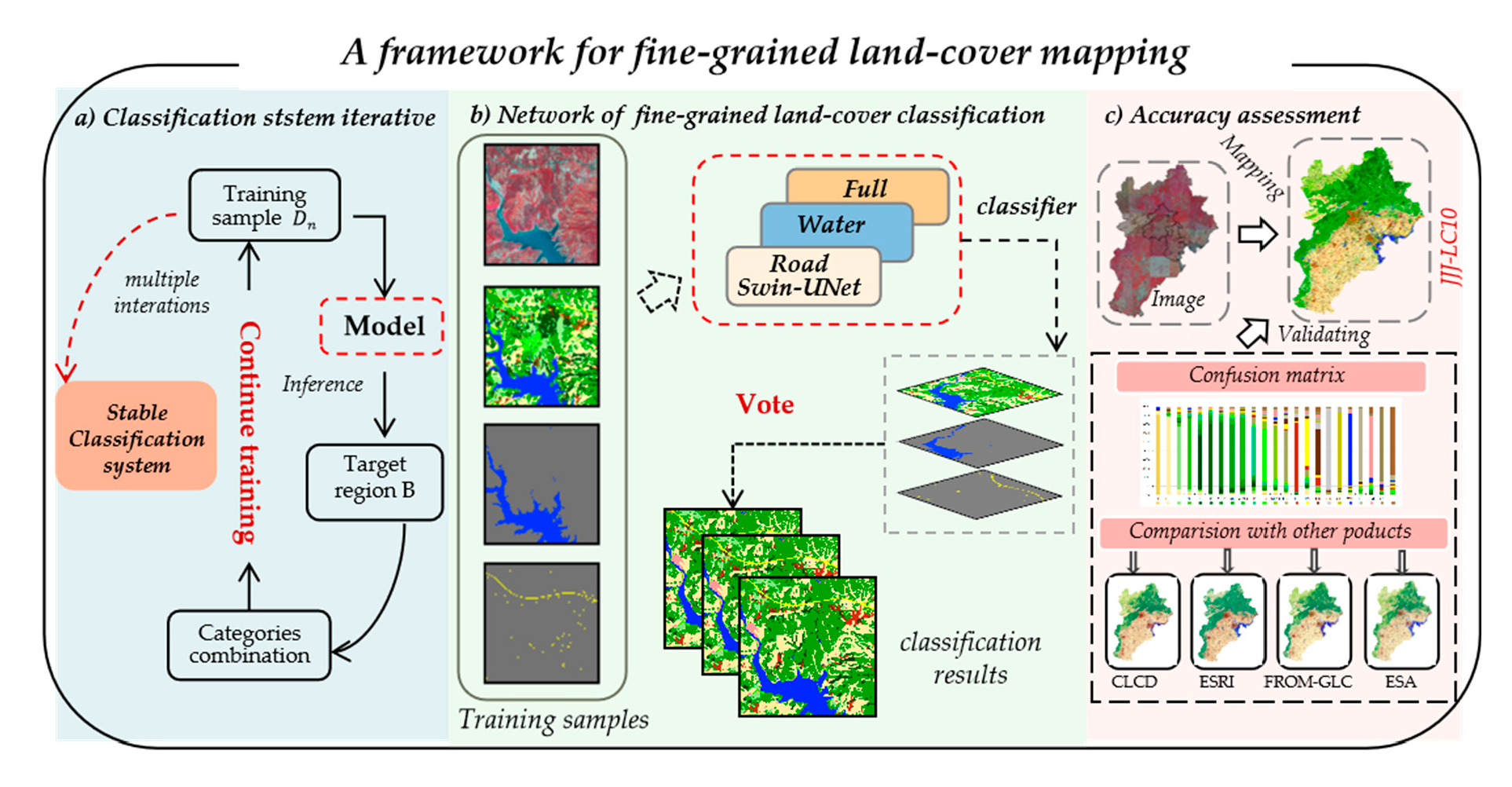
Figure 2 provides a detailed depiction of the proposed fine-grained land-cover classification mapping framework. This framework consists of three main parts: constructing a fine-grained land-cover deep learning network, an iterative optimization method for the classification system, accuracy assessment, and comparison with existing land-cover products. In the following sections, these three parts will be introduced in detail.
3.2. Deep Learning Network for Fine-Grained Land-Cover Classification
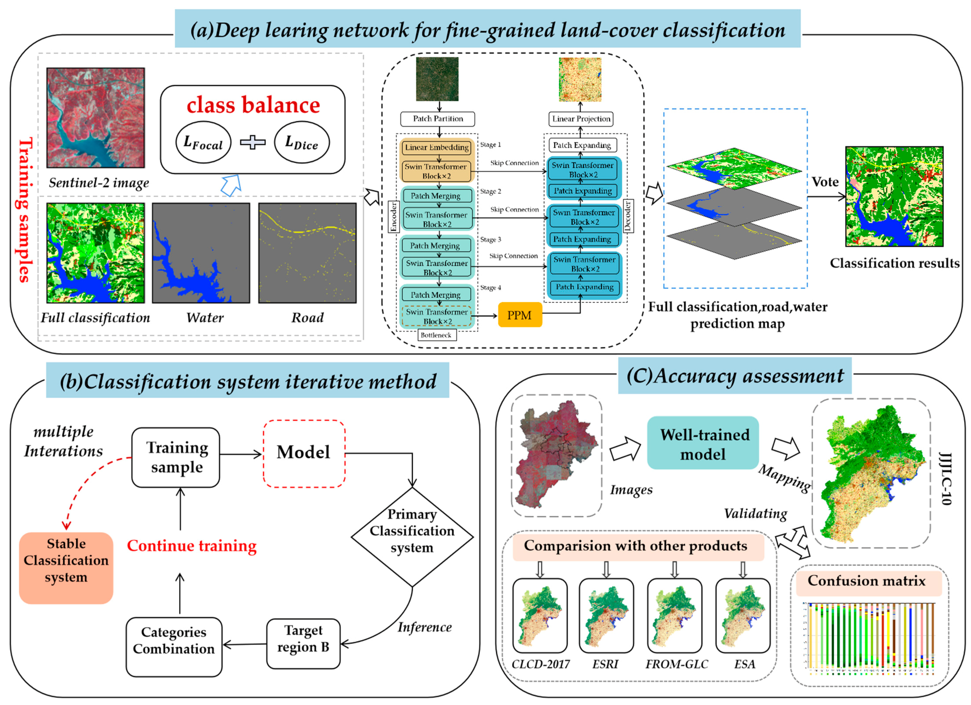
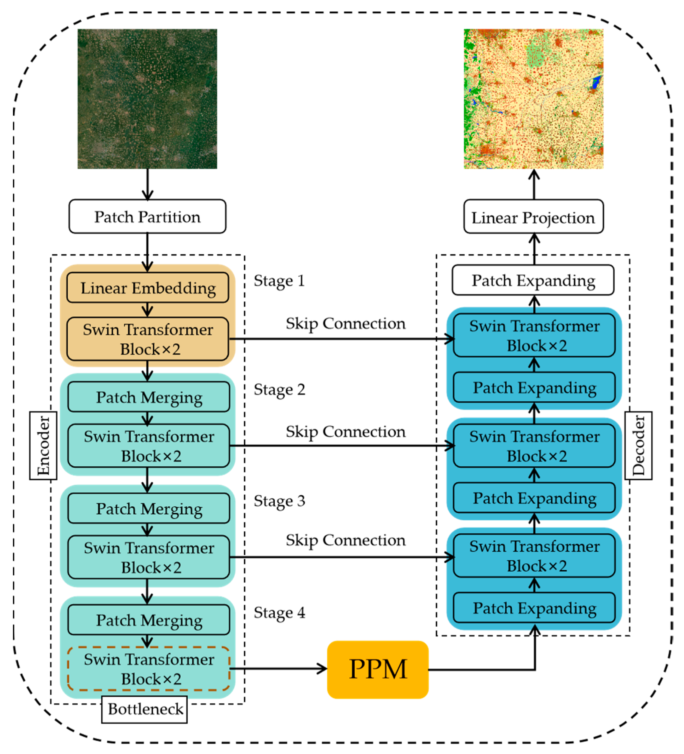
The network structure employed for fine-grained land-cover classification in this study is illustrated in Figure 3. To extract fine-grained feature information, we introduced a pyramid pooling module on the basis of Swin-UNet, enhancing the model’s capability to recognize features at different scales. To address the highly imbalanced sample data issue, a weighted combination loss function based on class balance was designed, further strengthening the model’s ability to learn rare categories. At the same time, with the aim of addressing the phenomenon of the weak connectivity of slender objects, we conducted independent model training using roads and water, and integrated the road, water, and full classification results according to the arrangement and combination method of natural objects, which improves the generalization ability of slender objects in complex scenes.
3.2.1. Swin-UNet Overview
The network mainly consists of an encoder, decoder, skip connection, and bottleneck. In the encoder part, the image with the size of 512 × 512 × 13 is inputted into the model, which is converted into a 4 × 4 size with non-overlapping patches using Patch Partition. The width and height of the image become a quarter of the original one, and the size of the channel becomes 16 times of the original one; thus, the size of the feature map obtained is 128 × 128 × 208. Then, when stacking the four stages to construct feature maps with different scales, firstly, the channel size of the feature map is projected to any dimension (denoted as C) using Liner Embedding. The other three stages are all composed of Patch Merging and Swin Transformer Block, where Swin Transformer Block is mainly used for feature extraction and Patch Merging is mainly used for down-sampling. After three consecutive layers of down-sampling, the height and width of the feature map are reduced by half each time, while the channel size is doubled, and the sizes of the output feature maps are 64 × 64 × 2C, 32 × 32 × 4C, and 16 × 16 × 8C, in that order.
The decoder incorporates patch-expanding layers that primarily perform upsampling on the deep features, doubling the dimensions of the feature maps in terms of width and height, while reducing the channel dimension to half of the original size. To restore the feature maps to the same size as the original image, in the final patch-expanding layer, the feature maps are directly upsampled four times in terms of width and height, while leaving the channel dimension unchanged, and then achieving pixel-level classification. Finally, the encoder’s multi-scale features and upsampled features are fused through skip connection, and the strategy effectively mitigates the loss of spatial details during the feature extraction process.
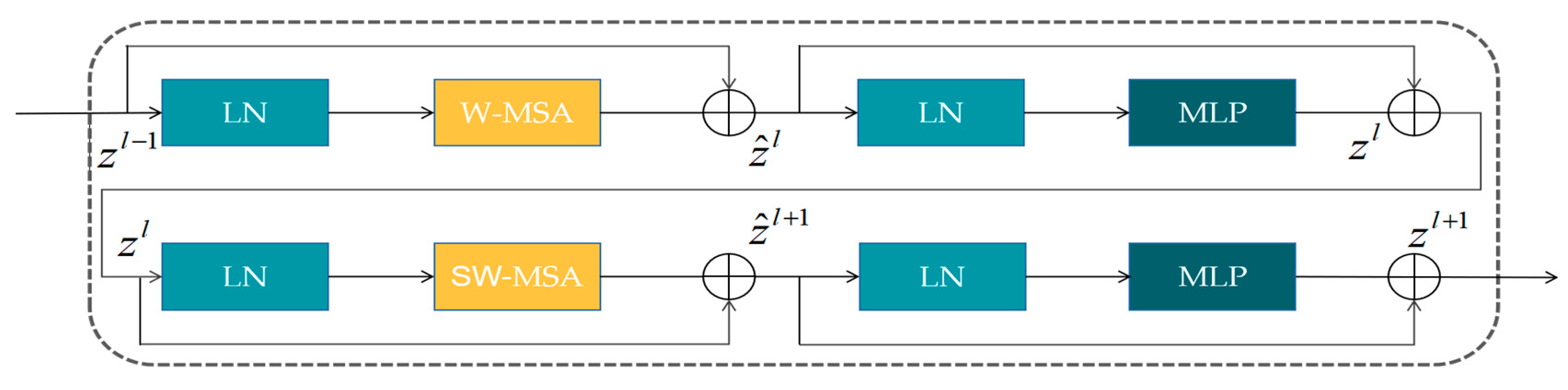
3.2.2. Swin Transformer Block
The network’s encoder, decoder, and bottleneck modules are implemented using the Swin Transformer block, as shown in Figure 4. Each Swin Transformer Block includes a LayerNorm (LN) layer, residual connections, multi-layer perceptron (MLP), and a multi-head self-attention (MSA) module. Among them, the Window-based Multihead Self-Attention (W-MSA) module is mainly used for feature extraction, while the shifted Window-based Multi-head Self-Attention (SW-MSA) module is responsible for establishing long-term spatial dependencies, facilitating global information interaction.
Two consecutive Swin Transformer Block formulas are computed as shown below. Firstly, the input feature to the stage is locally normalized (), and then it undergoes for global feature computation, followed by residual concatenation to generate the feature . Next, feature undergoes , , and residual concatenation to obtain the output feature of the first layer. The structure of the second layer is essentially similar to that of the first one, with the only distinction being the utilization of a different self-attention module.
where denotes the output features of the () module, denotes the output features of the module, and denotes the number of network layers.
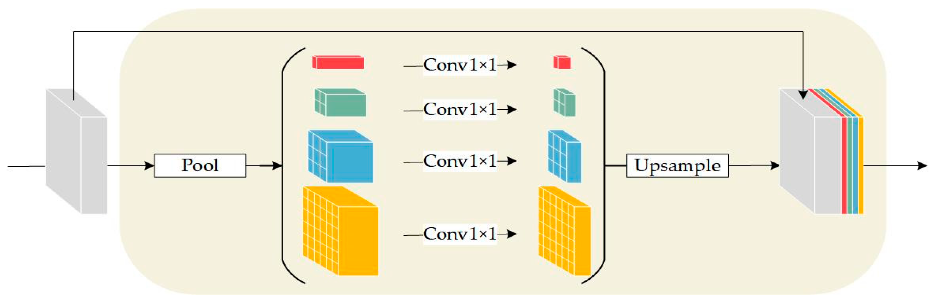
3.2.3. Pyramid Pool Module
Due to the large-scale differences and irregular shapes of different land objects in remote sensing images, the model needs to effectively extract land objects under different receptive fields. Larger land objects, typically containing more contextual information, require a broader global context to capture their overall features, such as forests and urban areas. Conversely, smaller land objects, due to their smaller scale, are more susceptible to local details. To accurately identify these smaller objects, a focus on finer local features is required, such as open-air stadiums and water bodies. Therefore, for different object scales, it is essential to judiciously utilize both global and local information.
The Pyramid Pooling Module (PPM) [39] combines multi-scale features by pooling feature maps at different scales to improve the model’s ability to obtain context information. We introduced the PPM module on the basis of Swin-UNet, so that the module can better capture the fine-grained features of small-scale features, thus improving the overall classification accuracy. As depicted in Figure 5, the feature maps generated by the encoder are subject to average pooling of varying sizes (1 × 1, 2 × 2, 3 × 3, 6 × 6), producing feature maps of different scales. Then, bilinear interpolation was employed to up-sample these feature maps, followed by their concatenation with the initial feature map. This process culminates in creating a multi-scale composite feature map, harmonizing the extraction of global semantic and local detail information.
3.2.4. Slender Feature Mapping Optimization
In large-scale land-cover classification tasks, the distribution of different land-cover scenes is highly complex, and different land-cover types exhibit significant morphological differences. Achieving an accurate classification of water and roads poses certain challenges compared to surface features. This is because, in remote sensing images, water and roads often exhibit relatively fine shapes, presenting a challenge for full classification models in extracting slender features. Additionally, conflicts between land features lead to discontinuities in water and roads, directly impacting the overall accuracy of land-cover products.
Considering the characteristics of the feature types, we trained the road and water models separately on the basis of the full classification model, and the overall process is shown in Figure 6. Among them, all of the parameters used in the training of the road and water models were consistent with those of the full classification model. By training a separate model for slender features, the model is more focused on learning and capturing the features of roads and water, which helps to improve the classification accuracy and product usability. Subsequently, we referred to the morphological permutations and combinations of natural features and used a voting algorithm to integrate the prediction results of roads and water into the full classification prediction results, thus improving the generalization ability of slender features in complex scenes.
3.2.5. Combination Loss Function Weighting Method Based on Class Balance
In land-cover classification tasks, an issue of imbalanced sample distribution is prevalent. This means that a minority of categories contain many sample data, while the majority have few sample data. The loss function assigns higher weights to categories with limited data, enhancing the model’s ability to learn from rare categories. The definition formula is as follows:
where represents the probability that a pixel belongs to class , is the balancing factor, and is the adjustment factor. In loss, is usually set to 0.25 and is set to 2. This is the optimal hyperparameter obtained by many experiments [40], which has shown good results in dealing with the problem of class imbalance.
At the same time, when facing complex geographical scenes, different land-cover types are prone to confusion, meaning that a single pixel can belong to multiple land-cover types simultaneously. The loss function considers the intersection between the true labels and the predicted results, providing a better approach to handling the issue of land-cover category confusion. The definition formula is as follows:
where represents the model’s predicted value, represents the true label value, and represents the intersection between the predicted result and the true label.
By combining the and loss functions, the accuracy of the model classification can be improved. However, due to the highly imbalanced data, the direct method of combining loss functions to balance the training samples does not produce satisfactory results. In addition, because of information overlap among the sample data, the model’s performance decreases with an increase in the number of samples. Cui et al. [41] proposed a class-balancing strategy, which involves re-weighting the loss based on the effective sample count to achieve class balance. The finite sample index is defined as , where represents the number of samples, represents the total number of samples, and represents the weight coefficient, which not only controls the growth rate, but also smoothly adjusts the weights of each category in the loss function. For example, a higher weight can be assigned to a category with a smaller number of samples, while a smaller weight can be assigned to a category with a larger number of samples, thus achieving a balanced treatment of categories.
Therefore, we devised a novel weighting scheme to readjust the losses based on the sample count for each land-cover type. The imbalance among sample data was mitigated by incorporating a normalized weighting factor. This strategic approach was integrated into the combined loss function to alleviate errors stemming from the overlap between the sample data. The calculation is outlined as follows
3.2.6. Experimental Settings
All experiments in this paper were conducted using the PyTorch deep learning framework. We trained the models using two NVIDIA RTX 3090 GPUs with 24 GB memory. At the same time, the training samples were enhanced via random cropping, random flipping, and random scaling images to improve the model’s generalization ability. Regarding the training model parameters, the AdamW optimizer was selected to train the model; the batch size was set to 4; the initial learning rate was set to 0.001; and the exponential decay strategy was used to reduce the learning rate gradually. The number of training iterations was set to 100 epochs.
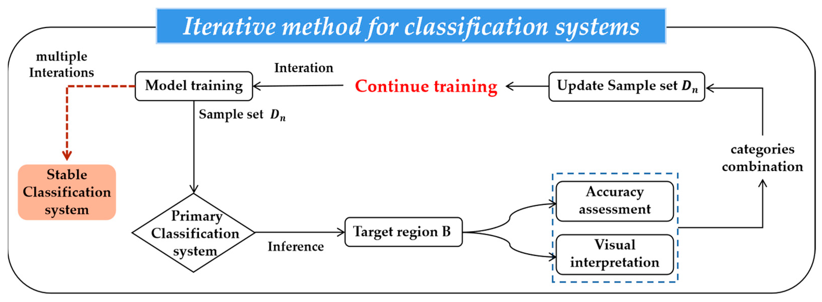
3.3. Classification System Iterative Method
This paper proposes a comprehensive method for optimizing fine-grained classification systems through deep iterative processes to explore the classification system in as much detail as possible at the 10 m scale. We employed multiple iterations and data feature mining through deep learning. Referring to the classification standard for Basic Geographic National Conditions Monitoring (CH/T 9029-2019) [19], published by the Ministry of Natural Resources of China, we gradually refined the classification system to improve the accuracy and stability of the model’s classification results.
The specific process is illustrated in Figure 7 and Algorithm 1, beginning with model training using sample dataset to establish the initial classification system. Subsequently, the well-trained initial model was employed to predict target data B, followed by a manual assessment and accuracy evaluation of the initial classification results. After thoroughly analyzing the discriminative capabilities and accuracy metrics for different land-cover types, we consolidated the categories with weak discriminative ability and low accuracy. The update of sample datasets accompanied this consolidation to optimize the initial classification system. Finally, we used the updated sample data to retrain the model and predict the target data B again to evaluate the model’s overall performance on the new classification system. We continued to iterate through the above steps until the most stable classification system was obtained.
| Algorithm 1: Stable classification system algorithm | |
| Input: Sample set with Primary Classes on target sensor and region ; classification network ; | |
| Output: Stable classes for target region and sensor; stable classification network ; | |
| 1: | train with |
| 2: | inference and evaluate on |
| 3: | calculate accuracy for |
| 4: | While do |
| 5: | |
| 6: | for do |
| 7: | if then |
| 8: | continue |
| 9: | else |
| 10: | |
| 11: | end for |
| 12: | end for |
| 13: | for |
| 14: | if then |
| 15: | combinate |
| 16: | update |
| 17: | update to |
4. Results
4.1. Accuracy Assessment Index
Evaluating the accuracy of land-cover products is critical in ensuring their credibility. The confusion matrix [42] is valuable for depicting the confusion between various land-cover types. It is one of the most prevalent methods in assessing the accuracy of land-cover products. Therefore, we used the confusion matrix method to calculate four accuracy evaluation metrics: overall accuracy (OA), user’s accuracy (UA), producer’s accuracy (PA), and kappa coefficient. These metrics were employed to assess the classification accuracy of the Beijing–Tianjin–Hebei land-cover product, and the calculation methods are as follows:
4.2. JJJLC-10:10 m Resolution Fine-Grained Land-Cover Map of the Beijing–Tianjin–Hebei Region
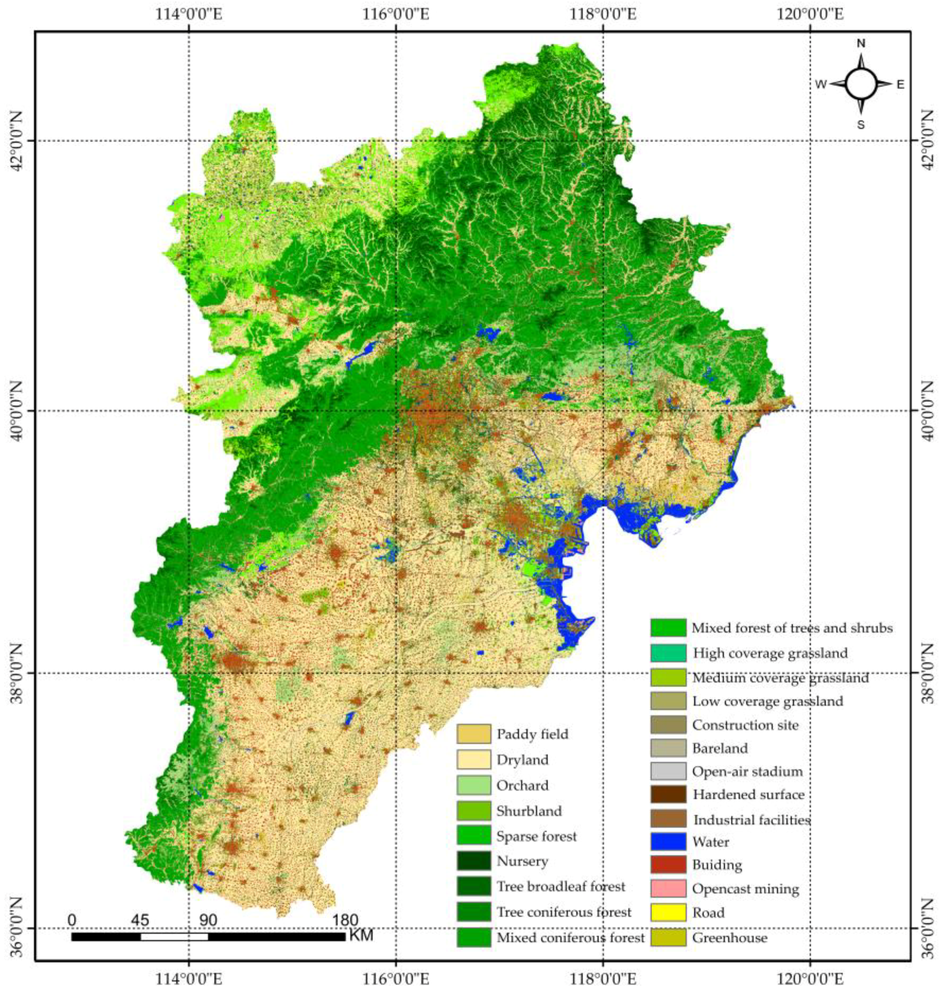
Figure 8 illustrates a fine-grained land-cover map of the Beijing–Tianjin–Hebei region with a 10 m resolution in 2017, containing 23 distinct land-cover types. The spatial distribution of the Beijing–Tianjin–Hebei region presents the following patterns: dense vegetation is mainly distributed in the northeastern part of the Taihang Mountains and the Yanshan region. Paddy fields and drylands are distributed primarily in the eastern coastal areas, the southeastern plains, and the northwestern plateau region of Zhangjiakou. Grasslands are mostly distributed in plateau and hilly regions, while built-up areas are concentrated in well-connected and densely populated plain areas. In general, the JJJLC-10 land-cover map accurately describes the spatial distribution of multiple land-cover types, which is highly consistent with the spatial pattern of land-cover in the Beijing–Tianjin–Hebei region.
Table 2 presents the area proportions of 23 distinct land-cover types. Dryland accounts for the largest proportion at 34.37%, followed closely by shrubland with a coverage of 24.33%. Dryland and shrubland, the main land-cover types in the Beijing–Tianjin–Hebei region, account for 58.7% of the total area. Following closely are buildings, broadleaf tree forests, high-coverage grasslands, orchards, and coniferous tree forests, accounting for 30.21% of the Beijing–Tianjin–Hebei region. Water, hardened surfaces, and roads are less common, amounting to 6.17% of the region’s area. The remaining land-cover types constitute 4.92% of the Beijing–Tianjin–Hebei region, with open-air stadiums having the smallest proportion at only 0.03%.
4.3. Accuracy Assessment of the JJJLC-10 Map
In this study, 4254 sample points were generated in the Beijing–Tianjin–Hebei region using stratified random sampling. The sample points were visualized and interpreted using a combination of Sentinel-2 imagery and Google Earth Pro to assess the accuracy of JJJLC-10 quantitatively. Because the JJJLC-10 land-cover product covers 23 land-cover types, the confusion matrix is divided into two parts in this paper: a Level I confusion matrix covering seven land-cover types and a Level II confusion matrix encompassing 23 fine-grained land-cover types. Table 3 summarizes the accuracy matrix for 23 fine-grained land-cover types. Overall, the JJJLC-10 land-cover product achieves an overall accuracy of 72.2% and a kappa coefficient of 0.706. From the perspective of PA, the open-air stadium land-cover type achieves the highest accuracy, reaching 92.7%. This is followed by the paddy field, dryland, greenhouse, construction site, water, nursery, and bareland types, all with accuracy rates of more than 80%. Land-cover types such as buildings, industrial facilities, shrublands, mixed coniferous forests, mixed forests of trees and shrubs, opencast mining, orchards, and tree broadleaf forests fall within the accuracy range of 60% to 70%. However, high-coverage grassland, medium-coverage grassland, low-coverage grassland, roads, and hardened surfaces show relatively lower accuracy, all below 60%. These results indicate that land-cover types occupying large areas in the Beijing–Tianjin–Hebei region exhibit relatively high accuracy. In addition, land-cover types with distinctive features also show higher precision. On the contrary, some land-cover types with small proportions and similar characteristics are easily confused, directly affecting classification accuracy.
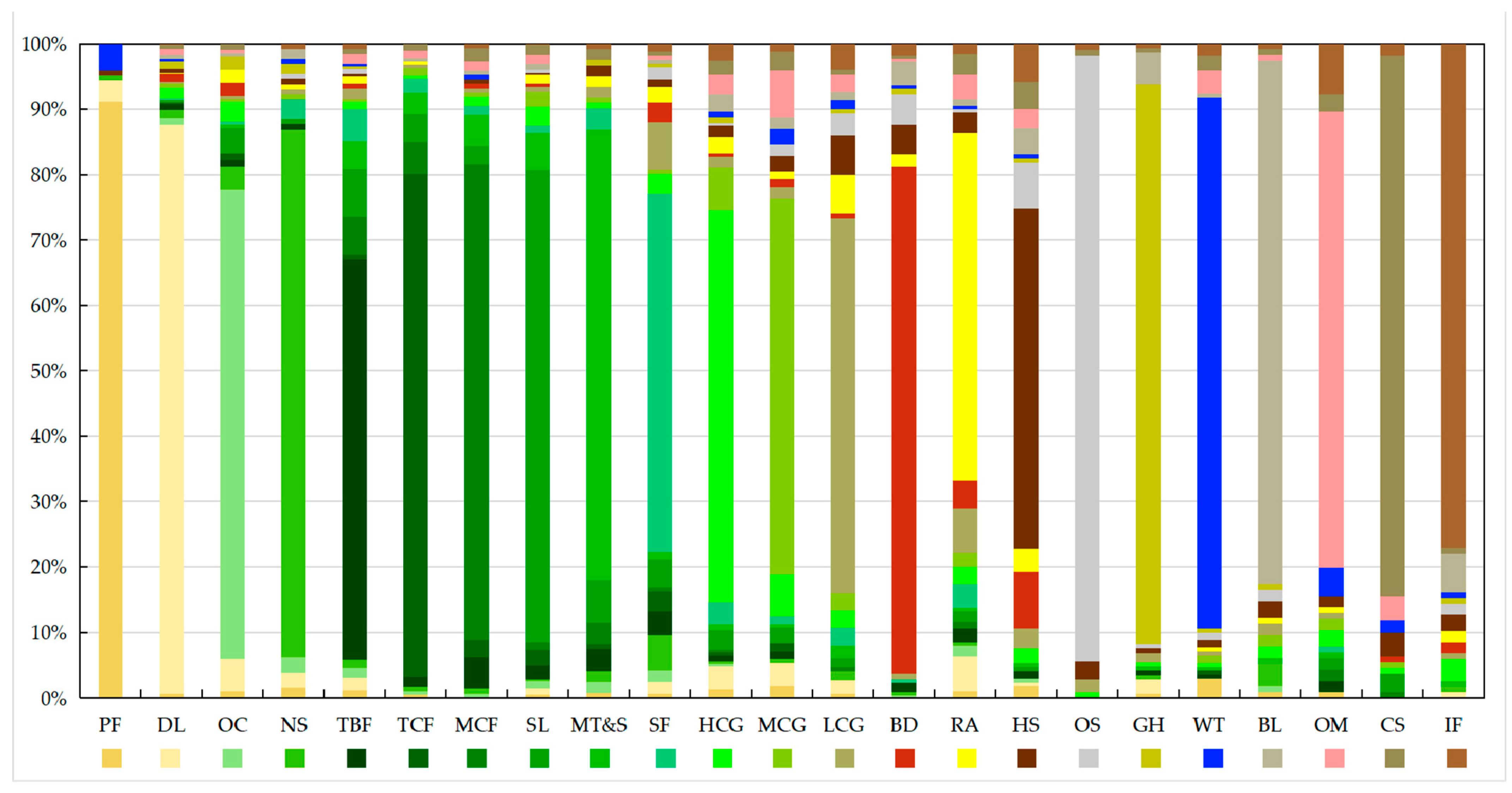
To visually illustrate the degree of confusion among the 23 fine-grained land-cover types, we calculated the proportion of confusion for these 23 different land-cover types, as shown in Figure 9. Firstly, hardened surfaces have the highest proportion of confusion, with roughly 48% of the validation samples being misclassified as other land-cover types, including buildings, industrial facilities, and construction sites. Roads are second only to hardened surfaces at about 47%. Because roads are inherently long and narrow features, they can be easily confused with the types of land-cover spread out on both sides of the road, with grasslands, drylands, and buildings accounting for the bulk of the confusion. Secondly, there is serious confusion between land-cover types with similar characteristics. For example, a number of shrublands, mixed coniferous forests, mixed forests of trees and shrubs, and sparse forests are misclassified as broadleaf tree forests. High-coverage grasslands, medium-coverage grasslands, and low-coverage grasslands also exhibit confusion with roads, water, and bareland. Due to the intrinsic diversity among grassland types, they often exhibit substantial similarities in terms of shape and characteristics, resulting in some degree of interclass confusion. However, most land-cover types such as paddy fields, open-air stadiums, water, and bareland are correctly classified, with only a minor portion experiencing misclassification errors.
In addition, Table 4 summarizes the accuracy matrix for seven major land-cover types in the Beijing–Tianjin–Hebei region. Combining fine-grained land-cover types with similar characteristics has significantly improved the classification accuracy, resulting in an overall accuracy of 80.3% and a kappa coefficient of 0.7602. Compared to the accuracy metrics in Table 3, the current classification differences are mainly concentrated in forest and impervious surface types. The average PA of forests and impervious surfaces increased from 0.644 to 0.768 and 0.726 to 0.859. This demonstrates the level of confusion between similar fine-grained land-cover types.
4.4. Comparison with Other Land-Cover Products
We conducted a quantitative assessment and visual validation on the four used land-cover products: CLCD-2017 [43], FROM-GLC10 [15], ESA_GLC10 [16], and ESRI_GLC10 [17]. Table 5 presents detailed information for the four land-cover products.
To better validate the accuracy and usability of JJJLC-10, we conducted a quantitative assessment using Level I validation samples for JJJLC-10, ESRI, FROM-GLC, ESA, and CLCD. Table 6 presents the overall accuracy (OA), kappa coefficient, user’s accuracy (UA), and producer’s accuracy (PA) for different categories of the compared products. The results indicate that JJJLC-10 exhibits the best performance, with an overall accuracy of 80.3% and a kappa coefficient of 76.02%. Following closely are ESA, FROM-GLC, and CLCD, with overall accuracies of 79.1%, 77.5%, and 75.9%, respectively. ESRI has the lowest overall accuracy at 69.5%, showing particularly low accuracy in categories such as forest, grassland, and bareland compared to the other products. In summary, JJJLC-10 demonstrates higher accuracy levels in the majority of categories compared to the other products.
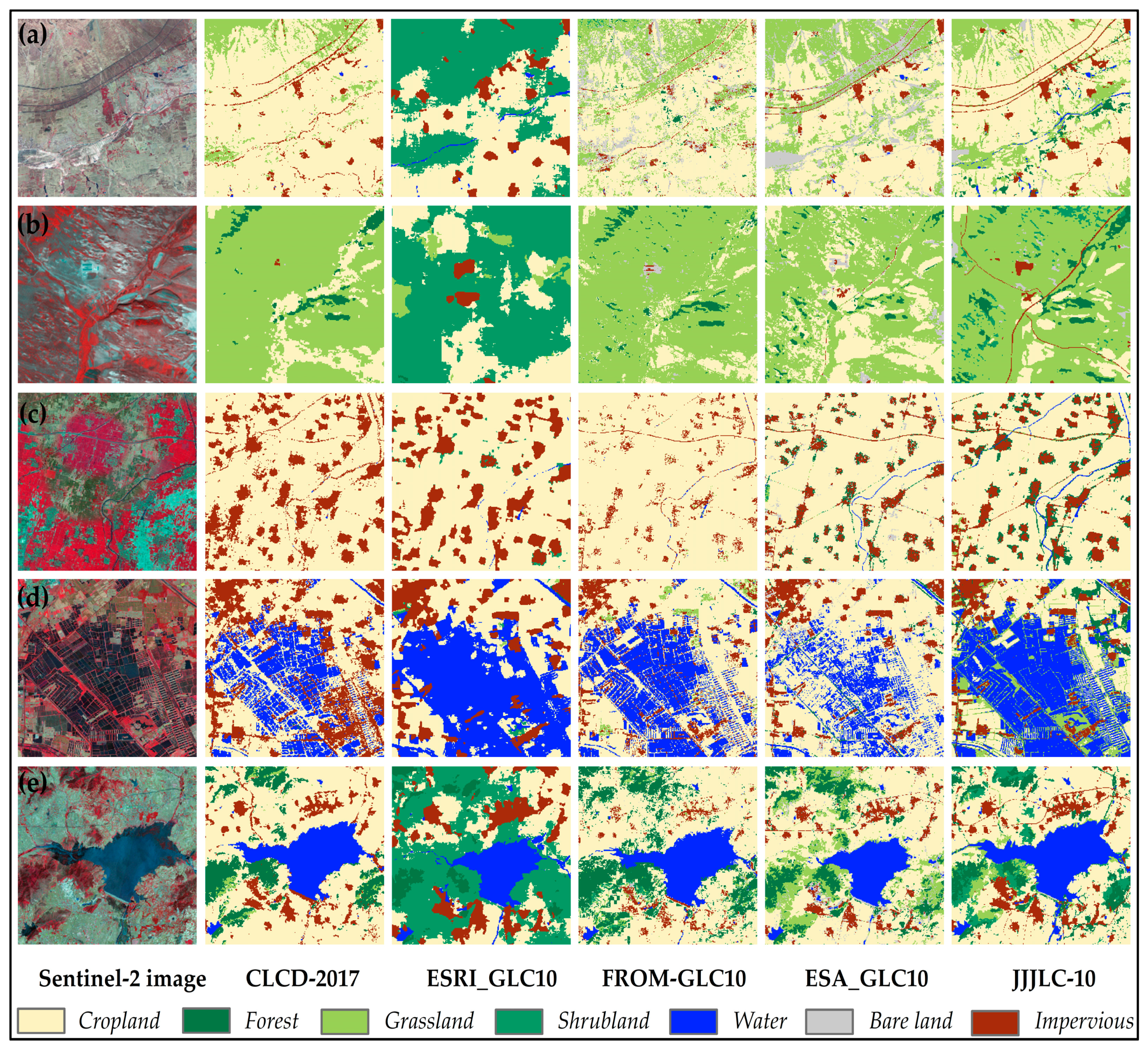
As illustrated in Figure 10, we selected five representative regions covering distinct landscape environments to demonstrate the overall performance of the JJJLC-10 land-cover product.
In general, JJJLC-10 exhibited high spatial consistency with the CLCD-2017, ESA_GLC10, and FROM-GLC10 land-cover products, providing a relatively accurate description of the spatial distribution of different land-cover types. In contrast, the ESRI_GLC10 land-cover product has the worst overall performance, with obvious confusion among cropland, forest, and grassland. It also exhibits unstable performance in transitional regions, such as the occurrence of evident patch effects when cropland transitions into grassland or forest. CLCD-2017, FROM-GLC10, and ESA_GLC10 demonstrated fine land-cover detail information but performed poorly on elongated land-cover types, such as roads and narrow rivers. Compared to these products, JJJLC-10 provides more accurate and fine-grained classification results and exhibits excellent performance in elongated land-cover types such as roads and rivers.
5. Discussion
5.1. Exploration of a Stable Classification System at 10 m Resolution
We employed the proposed deep iterative fine-grained classification system method to explore the classification system suitable for Sentinel-2 data. Through the repetitive training of the sample dataset and optimization of the classification system, we ultimately obtained the most stable classification system at this resolution.
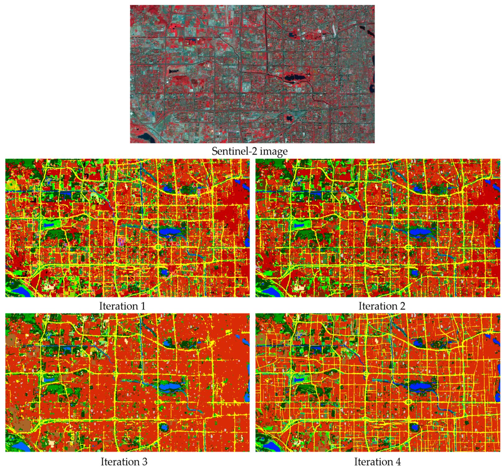
Figure 11 illustrates the land-cover classification results obtained at different iteration stages. In the first iteration, we used a sample dataset containing 91 land-cover types to train the model and establish the initial classification system. Then, using the trained initial model, we predicted the target area, manually interpreted and statistically analyzed the initial classification results, and merged categories that lacked discriminative capability at this resolution. Following this, we retrained the model using the streamlined classification system and predicted the target area again. In the second iteration, there was a significant salt-and-pepper effect between ground objects, especially in the building area. Due to the too-detailed division, the continuity of the road was hindered, resulting in the classification results showing fragmentation and unnatural visual effects. In the third iteration, we observed a reduction in the fragmentation of land-cover patches, yet the salt-and-pepper noise between land features still existed. There was noticeable confusion between land features with similar characteristics, and the representation of some slender features in the classification results lacked smoothness. Moving into the fourth iteration, we noticed a significant reduction in the salt-and-pepper effect, and the overall shape of the land-cover patches became more coherent. This change indicated that the gradual optimization of the classification system over the three iterations substantially enhanced the consistency and continuity of the land-cover classification results. We progressively optimized and streamlined the initial classification system through multiple iterations, ultimately constructing a stable classification system encompassing 23 land-cover types. This iterative process makes land-cover classification more detailed and accurate.
5.2. Slender Land-Cover Type Mapping Optimization
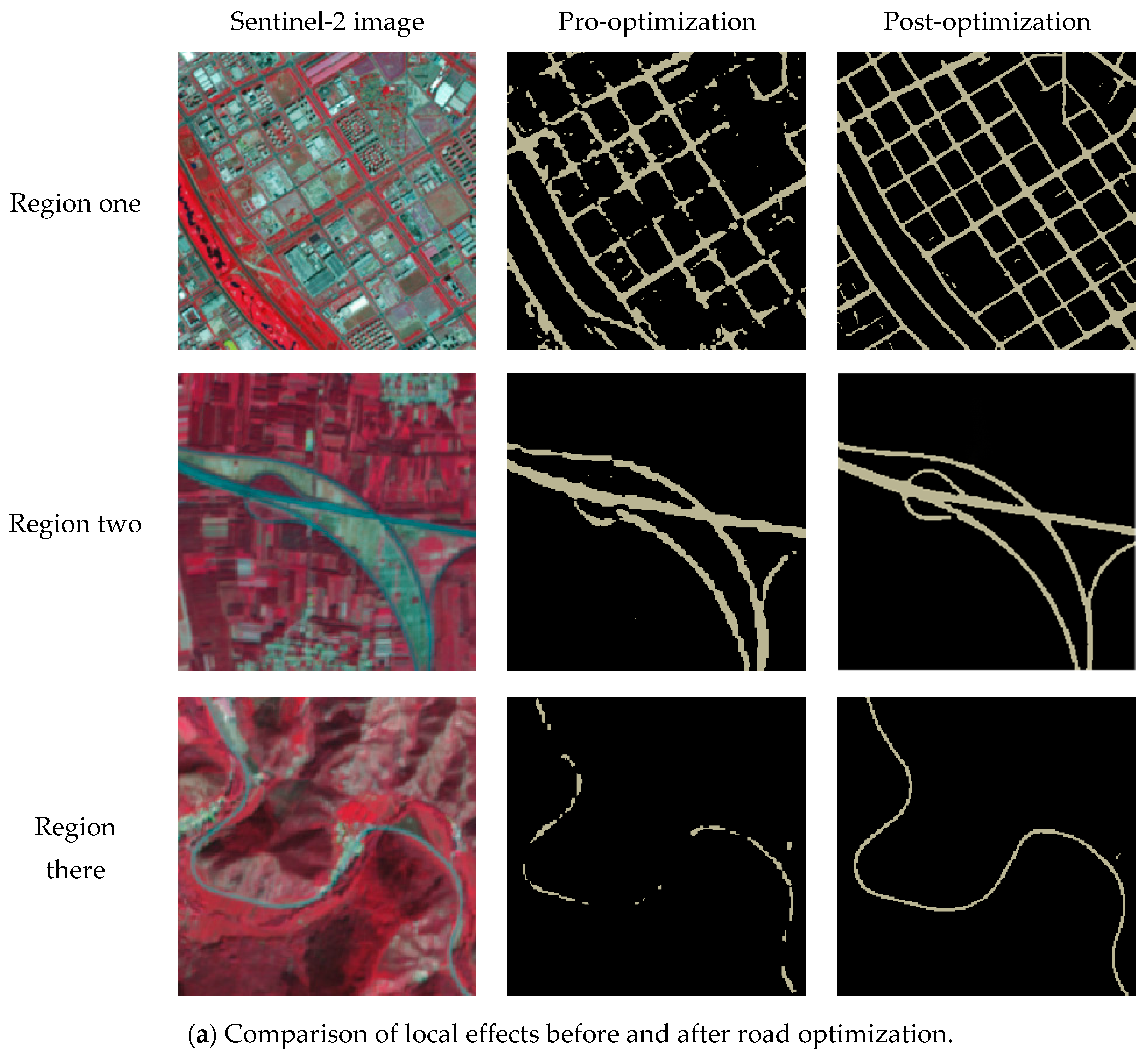
Firstly, the independent training of the inferior feature approach was used to optimize the slender land-cover type. Figure 12 presents the local effect comparisons before and after cartographic optimization. To demonstrate the reliability of the proposed method, three different road scenarios were selected for comparison. Region one depicts the complex urban road background due to the intricate distribution of roads and is easily affected by the surrounding buildings. This leads to the phenomenon of disconnection and adhesion of roads in the prediction process. After optimization, the optimized road connectivity is more robust and reduces the adhesion phenomenon between different roads, which is consistent with the real road information. Region two is the background area of overpasses, where the shadows of upper-level roads at road intersections can obscure lower-level roads, leading to the insufficient extraction of road detail information and consequential instances of missed detection. However, optimized road capture includes more local detail information and mitigates missed detection issues. Region three represents areas where roads are mixed with vegetation: roads are often obstructed by trees and shadows, making extraction challenging. However, the optimized results can almost completely extract obscured roads. Our method reduces the phenomenon of missed road detection and adhesion to a certain extent, thus ensuring the integrity and connectivity of the road.
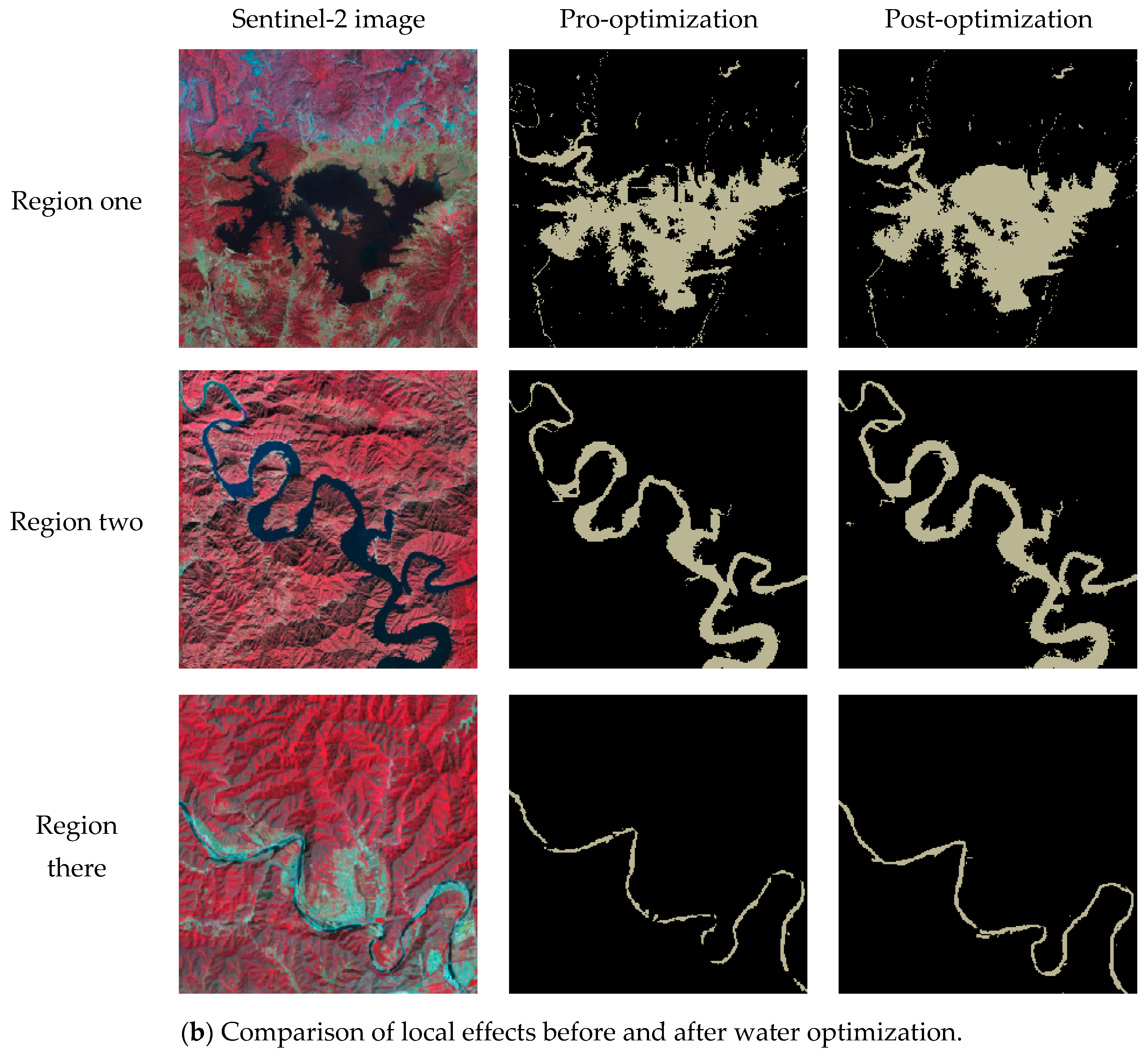
Three representative waters were selected for comparison. Region one is a large lake. Due to the presence of surrounding vegetation and shadows, the multi-classification model extraction is ineffective, resulting in a significant number of misclassifications. However, when more attention is paid to this category, the phenomenon of misclassification is improved. Region two is a large river whose shape is usually more complicated, showing curved or bifurcated shapes. This often leads to misclassification at the edge of the water body. However, the optimized visualization results are relatively complete. Region three consists of small rivers, where the surrounding vegetation and shadows significantly interfere with the classification of small rivers, resulting in disconnection. However, the small rivers can maintain their inherent shape after optimization. In general, the optimized results significantly improve the phenomenon of misclassification and disconnection and enhance the overall coherence of water.
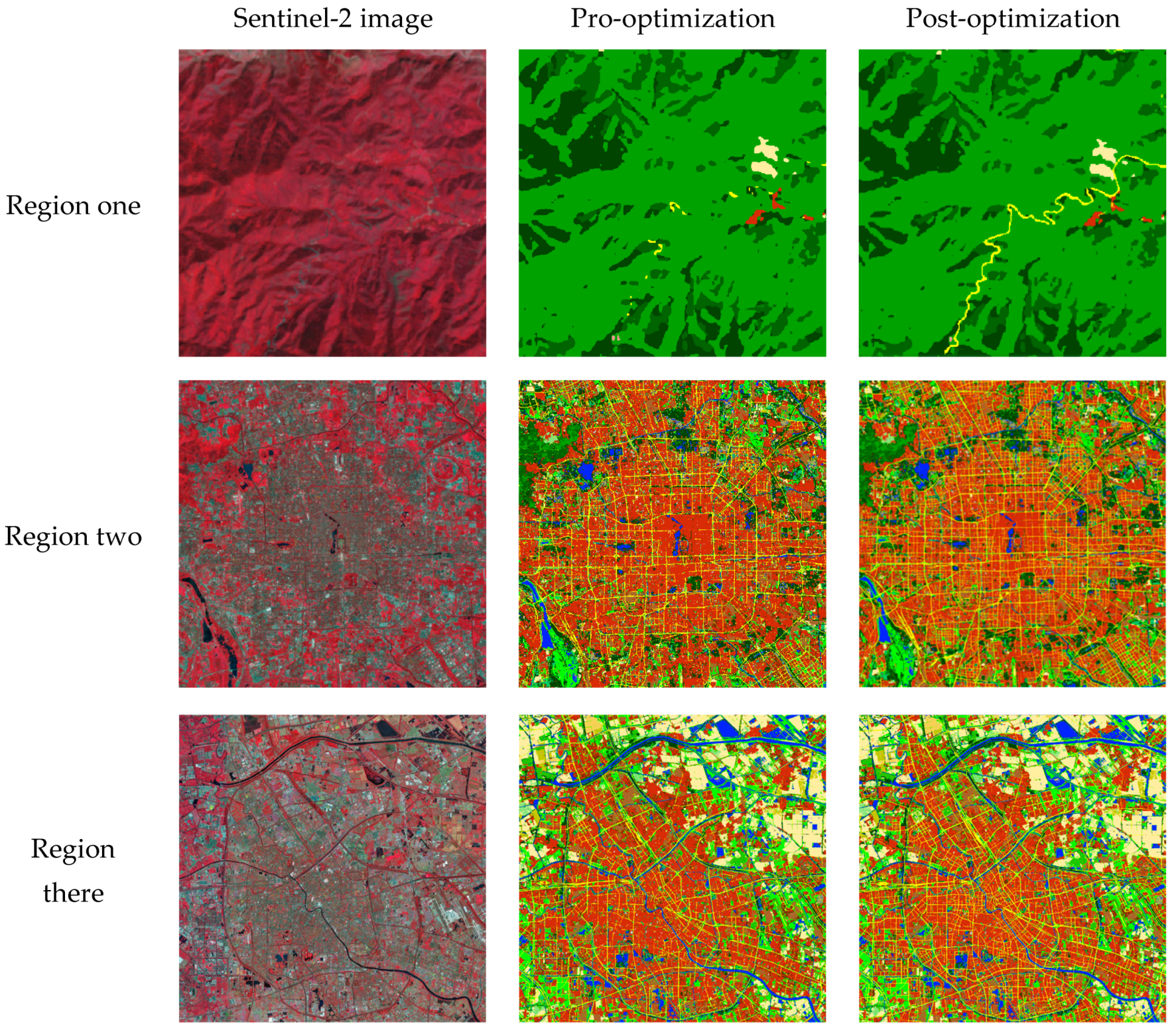
Secondly, we used the voting method to integrate the road and water prediction results into the multi-classification prediction results, which improved the generalization ability of slender objects in complex scenarios. Figure 13 illustrates the land-cover classification results before and after the integration of slender features, from which it can be seen that the problems of missed detection and disconnection of roads and water are effectively solved after the integration. The overall classification results are more in line with the real-world geographical scene distribution.
6. Conclusions
This paper proposes a mapping framework for fine-grained land-cover classification, aiming to produce large-scale land-cover products with fine-grained land-cover types. Firstly, we propose an iterative method for a fine-grained classification system, exploring a stable classification system tailored to a specific sensor for the target area. Through multiple iterations and the optimization of the classification system, we ultimately constructed a stable classification system for Sentinel-2 data, encompassing 23 land-cover types. Furthermore, we enhanced the model by introducing a pyramid pooling module on the basis of Swin-UNet and designed a combination loss function based on class balance. Additionally, while leveraging spatial relationships in natural features as clues, we used a voting algorithm to integrate predictions from the overall classification model and slender features. This approach addresses the challenges encountered in large-scale scenes, such as varying scales of target features, imbalanced sample quantities, and the weak connectivity of slender features.
To evaluate the performance of the proposed framework, we selected the 2017 Sentinel-2 image covering the Beijing–Tianjin–Hebei region as our experimental data. We produced the fine-grained land-cover product JJJLC-10 for this region, which covered 23 land-cover types. Subsequently, we conducted a validation of JJJLC-10 using a dataset comprising 4254 visually interpreted validation samples. The validation results demonstrate that within the I-level validation system, JJJLC-10 achieved an overall accuracy of 80.3% and a kappa coefficient of 0.7602, covering seven land-cover types. Within the II-level validation system, it achieved an overall accuracy of 72.2% and a kappa coefficient of 0.706, covering 23 land-cover types. Compared with the four land-cover products covering the Beijing–Tianjin–Hebei region, our analysis reveals that JJJLC-10 accurately represented the spatial distribution of various land-cover types, excelling in the classification of slender features like roads and water. Overall, JJJLC-10 exhibited significant advantages over 10 m resolution land-cover products in terms of classification quantity, classification accuracy, and spatial detail. In future research, we will continue our in-depth research to explore land-cover products with higher accuracy and more refined categories.
Author Contributions
Conceptualization, Z.Y. and Z.C.; methodology, X.Y. and Y.X.; validation, W.Z.; formal analysis, Z.Y.; resources, Z.C.; writing—original draft preparation, W.Z. and X.Y.; writing—review and editing, W.Z. and Y.X.; visualization, W.Z.; supervision, Y.X.; project administration, Z.C.; funding acquisition, Z.C. All authors have read and agreed to the published version of the manuscript.
Funding
This research was funded by the National Natural Science Foundation of China (No. 42071407); the Science and Disruptive Technology Research Pilot Fund of the Aerospace Information Innovation Institute, the Chinese Academy of Sciences (No. E3Z219010F); and the Open Fund of Key Laboratory of Urban Spatial Information, Ministry of Natural Resources, Grant No. 2023PT001.
Data Availability Statement
Data are contained within the article.
Acknowledgments
The authors are grateful to the editors and anonymous reviewers for their informative suggestions.
Conflicts of Interest
The authors declare no conflict of interest.
References
- Liu, X.; He, J.; Yao, Y.; Zhang, J.; Liang, H.; Wang, H.; Hong, Y. Classifying urban land use by integrating remote sensing and social media data. Int. J. Geogr. Inf. Sci. 2017, 31, 1675–1696. [Google Scholar] [CrossRef]
- Chen, P.; Huang, H.; Shi, W. Reference-free method for investigating classification uncertainty in large-scale land cover datasets. Int. J. Appl. Earth Obs. Geoinf. 2022, 107, 102673. [Google Scholar] [CrossRef]
- Running, S.W. Climate change. Ecosystem disturbance, carbon, and climate. Science 2008, 321, 652–653. [Google Scholar] [CrossRef]
- Hansen, M.C.; Defries, R.S.; Townshend, J.R.G.; Sohlberg, R. Global land cover classification at 1km spatial resolution using a classification tree approach. Int. J. Remote Sens. 2000, 21, 1331–1364. [Google Scholar] [CrossRef]
- Friedl, M.A.; Sulla-Menashe, D.; Tan, B.; Schneider, A.; Ramankutty, N.; Sibley, A.; Huang, X.M. MODIS Collection 5 global land cover: Algorithm refinements and characterization of new datasets. Remote Sens. Environ. 2010, 114, 168–182. [Google Scholar] [CrossRef]
- Bartholome, E.; Belward, A.S. GLC2000: A new approach to global land cover mapping from Earth observation data. Int. J. Remote Sens. 2005, 26, 1959–1977. [Google Scholar] [CrossRef]
- Arino, O.; Bicheron, P.; Achard, F.; Latham, J.; Witt, R.; Weber, J. The most detailed portrait of Earth. Eur. Space Agency 2008, 136, 25–31. [Google Scholar]
- Bicheron, P.; Leroy, M.; Brockmann, C.; Krämer, U.; Miras, B.; Huc, M.; Ninõ, F.; Defourny, P.; Vancutsem, C.; Arino, O. Globcover: A 300 m global land cover product for 2005 using ENVISAT MERIS time series. In Proceedings of the Recent Advances in Quantitative Remote Sensing Symposium, Valencia, Spain, 25–29 September 2006; pp. 538–542. [Google Scholar]
- Giri, C.; Pengra, B.; Long, J.; Loveland, T.R. Next generation of global land cover characterization, mapping, and monitoring. Int. J. Appl. Earth Obs. Geoinf. 2013, 25, 30–37. [Google Scholar] [CrossRef]
- Grekousis, G.; Mountrakis, G.; Kavouras, M. An overview of 21 global and 43 regional land-cover mapping products. Int. J. Remote Sens. 2015, 36, 5309–5335. [Google Scholar] [CrossRef]
- Gong, P.; Wang, J.; Le, Y.; Zhao, Y.; Zhao, Y. Finer resolution observation and monitoring of global land cover: First mapping results with Landsat TM and ETM+ data. Int. J. Remote Sens. 2013, 34, 2607–2654. [Google Scholar] [CrossRef]
- Zhang, X.; Liu, L.; Chen, X.; Gao, Y.; Xie, S.; Mi, J. GLC_FCS30: Global land-cover product with fine classification system at 30 m using time-series Landsat imagery. Earth Syst. Sci. Data. 2021, 13, 2753–2776. [Google Scholar] [CrossRef]
- Ding, Y.; Yang, X.; Wang, Z.; Fu, D.; Li, H.; Meng, D.; Zeng, X.; Zhang, J. A Field-Data-Aided Comparison of Three 10 m Land Cover Products in Southeast Asia. Remote Sens. 2022, 14, 5053. [Google Scholar] [CrossRef]
- Liu, S.; Wang, H.; Hu, Y.; Zhang, M.; Zhu, Y.; Wang, Z.; Li, D.; Yang, M.; Wang, F. Land Use and Land Cover Mapping in China Using Multi-modal Fine-grained Dual Network. IEEE Trans. Geosci. Remote Sens. 2023, 61, 4405219. [Google Scholar]
- Peng, G.; Han, L.; Meinan, Z.; Congcong, L.; Jie, W.; Huabing, H.; Nicholas, C.; Luyan, J.; Wenyu, L.; Yuqi, B.; et al. Stable classification with limited sample: Transferring a 30-m resolution sample set collected in 2015 to mapping 10-m resolution global land cover in 2017. Sci. Bull. 2019, 64, 370–373. [Google Scholar]
- Zanaga, D.; Van De Kerchove, R.; De Keersmaecker, W.; Souverijns, N.; Brockmann, C.; Quast, R.; Wevers, J.; Grosu, A.; Paccini, A.; Vergnaud, S. ESA WorldCover 10 m 2020 v100, Zenodo. 2021. Available online: https://zenodo.org/records/5571936/ (accessed on 21 September 2023).
- Karra, K.; Kontgis, C.; Statman-Weil, Z.; Mazzariello, J.C.; Mathis, M.; Brumby, S.P. Global land use/land cover with Sentinel 2 and deep learning. In Proceedings of the 2021 IEEE International Geoscience and Remote Sensing Symposium IGARSS, Brussels, Belgium, 11–16 July 2021; pp. 4704–4707. [Google Scholar]
- Di Gregorio, A. Land Cover Classification System: Classification Concepts and User Manual: LCCS; FAO: Rome, Italy, 2005. [Google Scholar]
- CH/T 9029-2019; Basic Geographic National Conditions Monitoring Content and Indicators. Standards Press of China: Beijing, China, 2019.
- Zhang, J.; Feng, Z.; Jiang, L. Progress on studies of land use/land cover classification systems. Resour. Sci. 2011, 33, 1195–1203. [Google Scholar]
- Chen, J.; Chen, J.; Gong, P.; Liao, A.; He, C. Higher resolution GLC mapping. Geomat. World 2011, 4, 12–14. [Google Scholar]
- Chen, J.; Chen, J.; Liao, A.; Cao, X.; Chen, L.; Chen, X.; He, C.; Han, G.; Peng, S.; Lu, M.; et al. Global land cover mapping at 30 m resolution: A POK-based operational approach. ISPRS-J. Photogramm. Remote Sens. 2015, 103, 7–27. [Google Scholar] [CrossRef]
- Giulia, C.; Paolo, D.F.; Pasquale, D.; Luca, C.; Marco, M.; Michele, M. Land Cover Mapping with Convolutional Neural Networks Using Sentinel-2 Images: Case Study of Rome. Land 2023, 12, 879. [Google Scholar]
- Zhang, L.; Zhang, L.; Du, B. Deep learning for remote sensing data: A technical tutorial on the state of the art. IEEE Geosci. Remote Sens. Mag. 2016, 4, 22–40. [Google Scholar] [CrossRef]
- Cai, Y.; Yang, Y.; Shang, Y.; Chen, Z.; Shen, Z.; Yin, J. IterDANet: Iterative intra-domain adaptation for semantic segmentation of remote sensing images. IEEE Trans. Geosci. Remote Sens. 2022, 60, 5629517. [Google Scholar] [CrossRef]
- Alem, A.; Kumar, S. Deep learning methods for land cover and land use classification in remote sensing: A review. In Proceedings of the 2020 8th International Conference on Reliability, Infocom Technologies and Optimization (Trends and Future Directions) (ICRITO), Noida, India, 4–5 June 2020; pp. 903–908. [Google Scholar]
- Xuemei, Z.; Lianru, G.; Zhengchao, C.; Bing, Z.; Wenzhi, L. Large-scale Landsat image classification based on deep learning methods. Apsipa Trans. Signal Inf. Proc. 2019, 8, e26. [Google Scholar]
- Huang, B.; Zhao, B.; Song, Y. Urban land-use mapping using a deep convolutional neural network with high spatial resolution multispectral remote sensing imagery. Remote Sens. Environ. 2018, 214, 73–86. [Google Scholar] [CrossRef]
- Liu, Y.; Mei, S.; Zhang, S.; Wang, Y.; He, M.; Du, Q. Semantic Segmentation of High-Resolution Remote Sensing Images Using an Improved Transformer. In Proceedings of the IGARSS 2022—2022 IEEE International Geoscience and Remote Sensing Symposium, Kuala Lumpur, Malaysia, 17–22 July 2022; pp. 3496–3499. [Google Scholar]
- Dosovitskiy, A.; Beyer, L.; Kolesnikov, A.; Weissenborn, D.; Zhai, X.; Unterthiner, T.; Dehghani, M.; Minderer, M.; Heigold, G.; Gelly, S. An image is worth 16x16 words: Transformers for image recognition at scale. arXiv 2020, arXiv:2010.11929. [Google Scholar]
- Liu, Z.; Lin, Y.; Cao, Y.; Hu, H.; Wei, Y.; Zhang, Z.; Lin, S.; Guo, B. Swin transformer: Hierarchical vision transformer using shifted windows. In Proceedings of the IEEE/CVF International Conference on Computer Vision, Montreal, QC, Canada, 10–17 October 2021; pp. 10012–10022. [Google Scholar]
- Cao, H.; Wang, Y.; Chen, J.; Jiang, D.; Zhang, X.; Tian, Q.; Wang, M. Swin-unet: Unet-like pure transformer for medical image segmentation. In Computer Vision—ECCV 2022 Workshops, Proceedings of the European Conference on Computer Vision, TEL Aviv, Israel, 23–27 October 2022; Springer: Cham, Switzerland, 2022; pp. 205–218. [Google Scholar]
- Yan, Y.; Chen, M.; Shyu, M.; Chen, S. Deep Learning for Imbalanced Multimedia Data Classification. In Proceedings of the 2015 IEEE International Symposium on Multimedia (ISM), Miami, FL, USA, 14–16 December 2015; pp. 483–488. [Google Scholar]
- Buda, M.; Maki, A.; Mazurowski, M.A. A systematic study of the class imbalance problem in convolutional neural networks. Neural Netw. 2018, 106, 249–259. [Google Scholar] [CrossRef] [PubMed]
- Yu, L.; Zhou, R.; Tang, L.; Chen, R. A DBN-based resampling SVM ensemble learning paradigm for credit classification with imbalanced data. Appl. Soft Comput. 2018, 69, 192–202. [Google Scholar] [CrossRef]
- Islam, M.T.; Islam, M.R.; Uddin, M.P.; Ulhaq, A. A Deep Learning-Based Hyperspectral Object Classification Approach via Imbalanced Training Samples Handling. Remote Sens. 2023, 15, 3532. [Google Scholar] [CrossRef]
- Zhao, X.; Cheng, Y.; Liang, L.; Wang, H.; Gao, X.; Wu, J. A balanced random learning strategy for CNN based Landsat image segmentation under imbalanced and noisy labels. Pattern Recognit. 2023, 144, 109824. [Google Scholar] [CrossRef]
- Abdi, A.M. Land cover and land use classification performance of machine learning algorithms in a boreal landscape using Sentinel-2 data. Gisci. Remote Sens. 2020, 57, 1–20. [Google Scholar] [CrossRef]
- Zhao, H.; Shi, J.; Qi, X.; Wang, X.; Jia, J. Pyramid scene parsing network. In Proceedings of the IEEE Conference on Computer Vision and Pattern Recognition, Honolulu, HI, USA, 21–26 July 2017; pp. 2881–2890. [Google Scholar]
- Lin, T.; Goyal, P.; Girshick, R.; He, K.; Dollár, P. Focal loss for dense object detection. IEEE Trans. Pattern Anal. Mach. Intell. 2017, 42, 318–327. [Google Scholar] [CrossRef]
- Cui, Y.; Jia, M.; Lin, T.; Song, Y.; Belongie, S. Class-Balanced Loss Based on Effective Number of Samples. In Proceedings of the 2019 IEEE/CVF Conference on Computer Vision and Pattern Recognition (CVPR), Long Beach, CA, USA, 15–20 June 2019; pp. 9260–9269. [Google Scholar]
- Olofsson, P.; Foody, G.M.; Stehman, S.V.; Woodcock, C.E. Making better use of accuracy data in land change studies: Estimating accuracy and area and quantifying uncertainty using stratified estimation. Remote Sens. Environ. 2013, 129, 122–131. [Google Scholar] [CrossRef]
- Yang, J.; Huang, X. The 30 m annual land cover dataset and its dynamics in China from 1990 to 2019. Earth Syst. Sci. Data 2021, 13, 3907–3925. [Google Scholar] [CrossRef]
Figure 1.
Geographical location and elevation map of Beijing–Tianjin–Hebei region in China.

Figure 2.
The overall framework of the fine-grained land-cover classification mapping.

Figure 3.
Network structure of fine-grained land-cover classification.

Figure 4.
Swin Transformer Block.

Figure 5.
Pyramid Pooling Module.

Figure 6.
Slender feature mapping optimization.

Figure 7.
Iterative method for classification system.

Figure 8.
JJJLC-10: Fine-grained land-cover map of Beijing–Tianjin–Hebei region.

Figure 9.
Percentage of confusion for 23 fine-grained land-cover types.

Figure 10.
Comparison between JJJLC-10 and other land-cover products. (a–e) shows five typical areas covering different landscape settings.
Figure 10.
Comparison between JJJLC-10 and other land-cover products. (a–e) shows five typical areas covering different landscape settings.

Figure 11.
The land-cover classification results were obtained at different iteration stages.

Figure 12.
Local comparison map before and after optimization of slender features. (a) shows the local effect comparison map before and after road optimization; (b) shows the local effect comparison map before and after water optimization.
Figure 12.
Local comparison map before and after optimization of slender features. (a) shows the local effect comparison map before and after road optimization; (b) shows the local effect comparison map before and after water optimization.


Figure 13.
Comparison of the effect before and after the integration of slender ground objects.


Table 1.
Introduction of Sentinel-2 data spectral band information.
| Band | Description | Resolution (m) | Wavelength (nm) |
|---|---|---|---|
| Band 1 | Aerosols | 60 | 443.9 |
| Band 2 | Blue | 10 | 496.6 |
| Band 3 | Green | 10 | 560 |
| Band 4 | Red | 10 | 664.5 |
| Band 5 | Red Edge 1 | 20 | 703.9 |
| Band 6 | Red Edge 2 | 20 | 740.2 |
| Band 7 | Red Edge 3 | 20 | 782.5 |
| Band 8 | NIR | 10 | 835.1 |
| Band 8A | Red Edge 4 | 20 | 864.8 |
| Band 9 | Water vapor | 60 | 945 |
| Band 10 | Cirrus | 60 | 1373.5 |
| Band 11 | SWIR 1 | 20 | 1613.7 |
| Band 12 | SWIR 2 | 20 | 2202.4 |
Table 2.
The area proportion of fine-grained land-cover types.
| Class Name | Proportion (%) | Class Name | Proportion (%) |
|---|---|---|---|
| Road | 1.78 | Opencast mining | 0.32 |
| Water | 2.94 | Open-air stadium | 0.03 |
| Orchard | 3.8 | Shrubland | 24.33 |
| Nursery | 0.59 | Sparse forest | 0.49 |
| Building | 8.35 | Broadleaf tree forest | 7.4 |
| Bareland | 0.08 | Coniferous tree forest | 3.22 |
| Dryland | 34.37 | Mixed coniferous forest | 0.1 |
| Paddy field | 0.65 | Mixed forest of trees and shrubs | 0.03 |
| Greenhouse | 0.54 | High-coverage grassland | 7.44 |
| Hardened surface | 1.45 | Medium-coverage grassland | 0.74 |
| Industrial facilities | 0.51 | Low-coverage grassland | 0.08 |
| Construction site | 0.76 |
Table 3.
The accuracy matrix for 23 fine-grained land-cover types.
| WF | DC | OC | NS | TBF | TCF | MCF | SL | MT&S | SF | HCG | MCG | LCG | BD | RA | HS | OS | GH | WT | BL | OM | CS | IF | Total | P.A. | |
|---|---|---|---|---|---|---|---|---|---|---|---|---|---|---|---|---|---|---|---|---|---|---|---|---|---|
| WF | 113 | 4 | 0 | 1 | 0 | 0 | 0 | 0 | 0 | 0 | 0 | 0 | 0 | 0 | 0 | 1 | 0 | 0 | 5 | 0 | 0 | 0 | 0 | 124 | 0.911 |
| DC | 3 | 414 | 5 | 6 | 4 | 1 | 0 | 2 | 0 | 1 | 8 | 3 | 1 | 6 | 1 | 3 | 0 | 5 | 2 | 3 | 4 | 3 | 1 | 476 | 0.870 |
| OC | 2 | 10 | 145 | 7 | 2 | 2 | 0 | 8 | 1 | 1 | 6 | 1 | 1 | 4 | 4 | 0 | 0 | 4 | 0 | 1 | 1 | 2 | 0 | 202 | 0.718 |
| NS | 2 | 3 | 3 | 105 | 1 | 0 | 0 | 1 | 0 | 4 | 0 | 1 | 1 | 0 | 1 | 1 | 1 | 2 | 1 | 2 | 0 | 0 | 1 | 130 | 0.808 |
| TBF | 3 | 5 | 4 | 3 | 160 | 2 | 15 | 19 | 11 | 13 | 3 | 1 | 4 | 2 | 3 | 1 | 2 | 1 | 1 | 0 | 4 | 2 | 2 | 261 | 0.613 |
| TCF | 1 | 0 | 1 | 1 | 3 | 143 | 9 | 8 | 6 | 4 | 1 | 2 | 1 | 0 | 1 | 0 | 0 | 0 | 0 | 1 | 2 | 2 | 0 | 186 | 0.769 |
| MCF | 0 | 0 | 1 | 1 | 7 | 4 | 107 | 4 | 7 | 2 | 2 | 1 | 1 | 1 | 0 | 1 | 0 | 0 | 1 | 1 | 2 | 3 | 1 | 147 | 0.728 |
| SL | 2 | 4 | 5 | 1 | 9 | 10 | 5 | 307 | 24 | 5 | 12 | 10 | 3 | 2 | 6 | 1 | 2 | 0 | 0 | 4 | 6 | 6 | 1 | 425 | 0.722 |
| MT&S | 1 | 0 | 2 | 2 | 4 | 1 | 4 | 8 | 84 | 4 | 1 | 1 | 2 | 0 | 2 | 2 | 0 | 1 | 0 | 0 | 0 | 2 | 1 | 122 | 0.689 |
| SF | 1 | 3 | 3 | 9 | 6 | 5 | 1 | 7 | 2 | 91 | 5 | 1 | 12 | 5 | 4 | 2 | 3 | 1 | 0 | 1 | 1 | 1 | 2 | 166 | 0.548 |
| HCG | 3 | 8 | 1 | 1 | 2 | 1 | 1 | 7 | 2 | 8 | 139 | 15 | 4 | 1 | 6 | 4 | 1 | 2 | 2 | 6 | 7 | 5 | 6 | 232 | 0.599 |
| MCG | 3 | 6 | 0 | 1 | 2 | 2 | 0 | 4 | 1 | 2 | 11 | 97 | 3 | 2 | 2 | 4 | 3 | 0 | 4 | 3 | 12 | 5 | 2 | 169 | 0.574 |
| LCG | 1 | 3 | 0 | 2 | 0 | 0 | 1 | 2 | 3 | 4 | 4 | 4 | 86 | 1 | 9 | 9 | 5 | 1 | 2 | 2 | 4 | 1 | 6 | 150 | 0.573 |
| BD | 0 | 0 | 1 | 1 | 3 | 0 | 0 | 0 | 0 | 1 | 0 | 0 | 2 | 170 | 4 | 10 | 10 | 2 | 1 | 8 | 1 | 1 | 4 | 219 | 0.776 |
| RA | 2 | 10 | 3 | 1 | 4 | 0 | 2 | 3 | 1 | 7 | 5 | 4 | 13 | 8 | 101 | 6 | 1 | 0 | 1 | 2 | 7 | 6 | 3 | 190 | 0.532 |
| HS | 3 | 1 | 1 | 0 | 2 | 0 | 0 | 1 | 1 | 0 | 4 | 0 | 5 | 15 | 6 | 89 | 12 | 1 | 1 | 7 | 5 | 7 | 10 | 171 | 0.520 |
| OS | 0 | 0 | 0 | 0 | 0 | 0 | 0 | 0 | 0 | 0 | 1 | 0 | 2 | 0 | 0 | 3 | 101 | 0 | 0 | 0 | 0 | 1 | 1 | 109 | 0.927 |
| GH | 1 | 3 | 0 | 1 | 1 | 0 | 0 | 0 | 1 | 0 | 1 | 0 | 2 | 0 | 0 | 1 | 1 | 125 | 0 | 7 | 0 | 1 | 1 | 146 | 0.856 |
| WT | 5 | 0 | 0 | 0 | 1 | 1 | 0 | 0 | 1 | 0 | 1 | 2 | 1 | 0 | 1 | 2 | 2 | 1 | 138 | 1 | 6 | 4 | 3 | 170 | 0.812 |
| BL | 1 | 0 | 1 | 4 | 0 | 0 | 0 | 0 | 1 | 0 | 2 | 2 | 2 | 0 | 1 | 3 | 2 | 1 | 0 | 92 | 1 | 1 | 1 | 115 | 0.800 |
| OM | 1 | 0 | 0 | 0 | 2 | 0 | 2 | 2 | 1 | 1 | 3 | 2 | 1 | 0 | 1 | 2 | 0 | 0 | 5 | 0 | 81 | 3 | 9 | 116 | 0.698 |
| CS | 0 | 0 | 0 | 0 | 0 | 0 | 1 | 3 | 0 | 0 | 1 | 1 | 0 | 1 | 0 | 4 | 0 | 0 | 2 | 0 | 4 | 91 | 2 | 110 | 0.827 |
| IF | 0 | 1 | 0 | 1 | 0 | 0 | 0 | 0 | 1 | 0 | 4 | 0 | 1 | 2 | 2 | 3 | 2 | 1 | 1 | 7 | 0 | 1 | 91 | 118 | 0.771 |
| Total | 148 | 475 | 176 | 148 | 213 | 172 | 148 | 386 | 148 | 148 | 214 | 148 | 148 | 220 | 155 | 152 | 148 | 148 | 167 | 148 | 148 | 148 | 148 | 4254 | |
| U.A. | 0.764 | 0.872 | 0.824 | 0.709 | 0.751 | 0.831 | 0.723 | 0.795 | 0.568 | 0.615 | 0.638 | 0.655 | 0.581 | 0.773 | 0.652 | 0.586 | 0.601 | 0.845 | 0.826 | 0.622 | 0.547 | 0.615 | 0.615 | ||
| O.A. | 0.722 | ||||||||||||||||||||||||
| Kappa | 0.706 | ||||||||||||||||||||||||
Note: WF = Water field; DC = Dry cropland; OC = Orchard; NS = Nursery; TBF = Tree broadleaf forest; TCF = Tree coniferous forest; MCF = Mixed coniferous forests; SL = Shrubland; MT&S = Mixed forests with trees and shrubs; SF = Sparse forest; HCG = High coverage grassland; MCG = Medium coverage grassland; LCG = Low coverage grassland; BD = Building; RA = Road; HS = Hardened surface; OS = Open-air stadium; GH = Greenhouse; WT = Water; BL = Bareland; OM = Opencast mining; CS = Construction site; IF = Industrial facilities.
Table 4.
The accuracy matrix for seven main land-cover types.
| CL | FST | SL | GL | IMP | WT | BL | Total | P.A. | |
|---|---|---|---|---|---|---|---|---|---|
| CL | 937 | 24 | 22 | 24 | 38 | 6 | 11 | 1062 | 0.882 |
| FST | 49 | 550 | 56 | 25 | 29 | 3 | 4 | 716 | 0.768 |
| SL | 23 | 40 | 417 | 20 | 21 | 0 | 8 | 529 | 0.788 |
| GL | 48 | 31 | 20 | 398 | 61 | 7 | 34 | 599 | 0.664 |
| IMP | 31 | 21 | 9 | 23 | 789 | 7 | 38 | 918 | 0.859 |
| WT | 6 | 6 | 1 | 8 | 13 | 136 | 12 | 182 | 0.747 |
| BL | 1 | 9 | 9 | 12 | 20 | 8 | 189 | 248 | 0.762 |
| Total | 1095 | 681 | 534 | 510 | 971 | 167 | 296 | 4254 | |
| U.A. | 0.856 | 0.808 | 0.781 | 0.78 | 0.813 | 0.814 | 0.639 | ||
| O.A. | 0.803 | ||||||||
| Kappa | 0.7602 | ||||||||
Note: CL = Cropland, FST = Forest, SL = Shrubland, GL = Grassland, IMP = Impervious surface, WT = Water, and BL = Bareland.
Table 5.
The detailed information of four land-cover products.
| Land-Cover Products | Resolution | Classification System | Data Source | Classification Method |
|---|---|---|---|---|
| CLCD | 30 m | 9 | Landsat-8 | Random forest classifier |
| FROM-GLC | 10 m | 10 | Sentinel-2 | Random forest classifier |
| ESA_GLC | 10 m | 11 | Sentinel-1, Sentinel-2 | Deep learning |
| ESRI_GLC | 10 m | 10 | Sentinel-2 | Deep learning (UNet) |
Table 6.
Comparison of mapping accuracy based on Level I validation samples.
| CL | FST | SL | GL | IMP | WT | BL | OA | Kappa | ||
|---|---|---|---|---|---|---|---|---|---|---|
| JJJ-LC10 | UA | 0.856 | 0.808 | 0.781 | 0.78 | 0.813 | 0.814 | 0.639 | 0.803 | 0.7602 |
| PA | 0.882 | 0.768 | 0.788 | 0.664 | 0.859 | 0.747 | 0.762 | |||
| ESRI | UA | 0.798 | 0.648 | 0.684 | 0.590 | 0.713 | 0.737 | 0.541 | 0.695 | 0.631 |
| PA | 0.859 | 0.687 | 0.639 | 0.512 | 0.814 | 0.559 | 0.6438 | |||
| FROM-GLC | UA | 0.814 | 0.752 | 0.798 | 0.751 | 0.815 | 0.749 | 0.564 | 0.775 | 0.727 |
| PA | 0.893 | 0.808 | 0.741 | 0.616 | 0.872 | 0.644 | 0.515 | |||
| ESA | UA | 0.824 | 0.780 | 0.822 | 0.737 | 0.819 | 0.760 | 0.652 | 0.791 | 0.746 |
| PA | 0.898 | 0.8812 | 0.742 | 0.660 | 0.874 | 0.668 | 0.578 | |||
| CLCD | UA | 0.807 | 0.731 | 0.785 | 0.692 | 0.799 | 0.731 | 0.561 | 0.759 | 0.705 |
| PA | 0.901 | 0.781 | 0.734 | 0.597 | 0.854 | 0.619 | 0.452 | |||
Note: CL = Cropland, FST = Forest, SL = Shrubland, GL = Grassland, IMP = Impervious surface, WT = Water, and BL = Bareland.
Disclaimer/Publisher’s Note: The statements, opinions and data contained in all publications are solely those of the individual author(s) and contributor(s) and not of MDPI and/or the editor(s). MDPI and/or the editor(s) disclaim responsibility for any injury to people or property resulting from any ideas, methods, instructions or products referred to in the content. |
© 2024 by the authors. Licensee MDPI, Basel, Switzerland. This article is an open access article distributed under the terms and conditions of the Creative Commons Attribution (CC BY) license (https://creativecommons.org/licenses/by/4.0/).
Share and Cite
MDPI and ACS Style
Zhang, W.; Yang, X.; Yuan, Z.; Chen, Z.; Xu, Y. A Framework for Fine-Grained Land-Cover Classification Using 10 m Sentinel-2 Images. Remote Sens. 2024, 16, 390. https://doi.org/10.3390/rs16020390
AMA Style
Zhang W, Yang X, Yuan Z, Chen Z, Xu Y. A Framework for Fine-Grained Land-Cover Classification Using 10 m Sentinel-2 Images. Remote Sensing. 2024; 16(2):390. https://doi.org/10.3390/rs16020390
Chicago/Turabian StyleZhang, Wenge, Xuan Yang, Zhanliang Yuan, Zhengchao Chen, and Yue Xu. 2024. "A Framework for Fine-Grained Land-Cover Classification Using 10 m Sentinel-2 Images" Remote Sensing 16, no. 2: 390. https://doi.org/10.3390/rs16020390
Note that from the first issue of 2016, this journal uses article numbers instead of page numbers. See further details here.