


Evaluating the Reconstructed All-Weather Land Surface Temperature for Urban Heat Island Analysis
by
Xuepeng Zhang
1,
Chunchun Meng
2,*,
Peng Gou
1,
Yingshuang Huang
1,
Yaoming Ma
3,
Weiqiang Ma
3,
Zhe Wang
4 and
Zhiheng Hu
5 1
Research Center of Big Data Technology, Nanhu Laboratory, Jiaxing 314000, China
2
Institute of Urban Meteorology, Beijing 100089, China
3
Institute of Tibetan Plateau Research, Chinese Academy of Sciences, Beijing 100101, China
4
School of Urban Planning and Design, Peking University Shenzhen Graduate School, Peking University, Shenzhen 518055, China
5
China Centre for Resources Satellite Data and Application, Beijing 100094, China
*
Author to whom correspondence should be addressed.
Remote Sens. 2024, 16(2), 373; https://doi.org/10.3390/rs16020373
Submission received: 7 November 2023
/
Revised: 11 January 2024
/
Accepted: 12 January 2024
/
Published: 17 January 2024
(This article belongs to the Special Issue Application of Remote Sensing-Based Monitoring of Local Climate in Urban Areas)
Abstract
:With the continuous improvement of urbanization levels in the Lhasa area, the urban heat island effect (UHI) has seriously affected the ecological environment of the region. However, the satellite-based thermal infrared land surface temperature (LST), commonly used for UHI research, is affected by cloudy weather, resulting in a lack of continuous spatial and temporal information. In this study, focusing on the Lhasa region, we combine simulated LST data obtained by the Weather Research and Forecasting (WRF) model with remote sensing-based LST data to reconstruct the all-weather LST for March, June, September, and December of 2020 at a resolution of 0.01° while using the Moderate-Resolution Imaging Spectroradiometer (MODIS) LST as a reference (in terms of accuracy). Subsequently, based on the reconstructed LST, an analysis of the UHI was conducted to obtain the spatiotemporal distribution of UHI in the Lhasa region under all-weather LST conditions. The results demonstrate that the reconstructed LST effectively captures the expected spatial distribution characteristics with high accuracy, with an average root mean square error of 2.20 K, an average mean absolute error of 1.51 K, and a correlation coefficient consistently higher than 0.9. Additionally, the heat island effect in the Lhasa region is primarily observed during the spring and winter seasons, with the heat island intensity remaining relatively stable in winter. The results of this study provide a new reference method for the reconstruction of all-weather LST, thereby improving the research accuracy of urban thermal environment from the perspective of foundational data. Additionally, it offers a theoretical basis for the governance of UHI in the Lhasa region.
1. Introduction
Land surface temperature (LST) is an important parameter for studying surface energy balance and land processes [1], and it serves as a fundamental dataset for exploring the surface urban heat island effect (UHI, the following UHI refers to the surface UHI) [2,3]. With the increasing level of urbanization in recent years, UHI has become a significant environmental governance issue, and obtaining high-precision LST is a prerequisite for accurately exploring UHI [4].
The conventional method to obtain the LST involves meteorological station and remote sensing (RS) observation data. However, the meteorological station distribution is relatively sparse, and the LST can exhibit significant variations within short distances [5]. Obtaining the LST through RS observation techniques offers high spatial coverage and easy accessibility, demonstrating a tremendous potential [6]. With the maturation of satellite thermal infrared technology, accessing LST data has become increasingly easier, and the accuracy of LST retrieval has gradually improved [7]. In particular, Moderate-Resolution Imaging Spectroradiometer (MODIS) product data, which have a short revisit period and global coverage, are commonly used in various research fields [8,9]. MODIS LST products have been widely applied in various research fields, including urban thermal environment analyses, agricultural drought assessments, and hydrological model simulations [10,11]. Nevertheless, the presence of clouds and rainfall can affect satellite TIR measurements, resulting in a lack of spatiotemporal continuity in LST imagery. Therefore, this incompleteness diminishes its value as foundational research data, or renders it entirely unusable.
Currently, there are four commonly used methods for LST reconstruction: spatiotemporal information-based methods, passive microwave methods, physical model-based methods and machine learning-based methods. Spatiotemporal information-based methods, including time interpolation algorithms, spatial interpolation algorithms, and interpolation algorithms that utilize both time and spatial information, involve the use of the geographical principle of similarity and proximity to interpolate clear-sky LST pixels that are temporally and spatially adjacent, thus obtaining pixels with clouds [12,13]. Common interpolation methods include inverse distance weighting [14], spline function [15], and kriging interpolation methods [16]. The accuracy of interpolation methods decreases with increasing range of missing pixels, so they are only applicable for reconstructing images with few cloud pixels. The passive microwave method can be used to directly retrieve all-weather LST data by penetrating cloud layers and obtaining surface information [17]. However, the spatial resolution of the LST data obtained by this method is relatively low, and the microwave signal significantly varies with surface characteristics; hence, the data are generally applied as supplementary data for LST generation [7,18]. The physical model method aims to construct mathematical equations based on physical principles and has become an important method for obtaining remote sensing data products [19]. The widely used physical model methods include the surface energy balance method and its derivatives [20,21], which can provide data that are as close to the true values as possible. However, there is often high uncertainty due to the difficulty in determining certain parameters. In recent years, artificial intelligence technology has continuously advanced and has been extensively applied in various fields, including research on LST reconstruction [22,23,24]. This method aims to establish relationships between internal features based on the initial data or observations to discover predictive patterns. LST reconstruction based on this method is also currently a commonly used approach, as it offers an efficient modeling approach that does not require the consideration of specific relationships between variables. Moreover, it has achieved remarkable achievements in terms of accuracy [24,25,26]. The method employed in this study for LST reconstruction involves the utilization of the Random Forest (RF) model, which is a flexible and stable machine learning model and is commonly used for generating various remote sensing products [27,28].
The new generation of the mesoscale WRF model can be used to simulate the surface skin temperature (TSK) that is very close to the LST through real final reanalysis (FNL) data. In fact, some researchers have even directly used the TSK as a substitute for the LST [29,30] Although the TSK derived from WRF simulations lacks the spatial details and accuracy of the satellite remote sensing-based LST (actual observations), it exhibits the characteristic of all-weather availability. This is also the reason why the WRF-simulated TSK (WRF LST) is used in this study. Furthermore, according to related studies, certain multisource remote sensing observation data can affect the variation in the LST, such as the digital elevation model (DEM) [31], normalized difference vegetation index (NDVI) [32], and latitude (LAT) [33]. Based on the above ideas, this paper combines the WRF model with the Random Forest mode, further combining multisource remote sensing observation data to ultimately obtain all-weather LST.
Urbanization causes significant changes in land within urban areas and frequent human activities, leading to the global issue of UHI, which results in the gradual deterioration of the thermal environment and severely affects urban ecological environment and public health [34]. The UHI has become one of the most frequent and influential climate disasters, and studying the UHI accurately by providing all-weather LST has become a hot topic [4]. Examples include the changes in UHI in Hangzhou City [35], the spatiotemporal patterns of UHI in Beijing [36], and the prediction of nocturnal UHI variations in the United Kingdom [37]. This study takes the Lhasa region in China as the study area, which includes Chengguan District and seven counties: Dazi, Duilongdeqing, Qushui, Linzhou, Mozhu-gongka, Nimu, and Dangxiong. Many scholars have also conducted research on the thermal environment in this area and have reached several conclusions. For instance, it is noted that Lhasa is one of the cities experiencing the most intense warming on the Qinghai–Tibet Plateau [38]. Additionally, urban expansion has a significant impact on the increase in average temperature in this region [39]. In recent years, changes in the urban ecology and climate environment (Figure 1d) in Lhasa have attracted much attention. According to related studies [40], the urban thermal environment issues in this area are becoming increasingly serious, requiring urgent research on UHI effects. Based on these remote sensing data and the WRF LST, we reconstruct the all-weather LST using the RF model, with the MODIS LST serving as a reference in terms of accuracy. Additionally, the reconstructed LST is used to analyze the UHI effect in the study area for the months of March, June, September, and December 2020, which is important for exploring the ecological and sustainable changes in the region.
2. Study Area and Datasets
2.1. Study Area
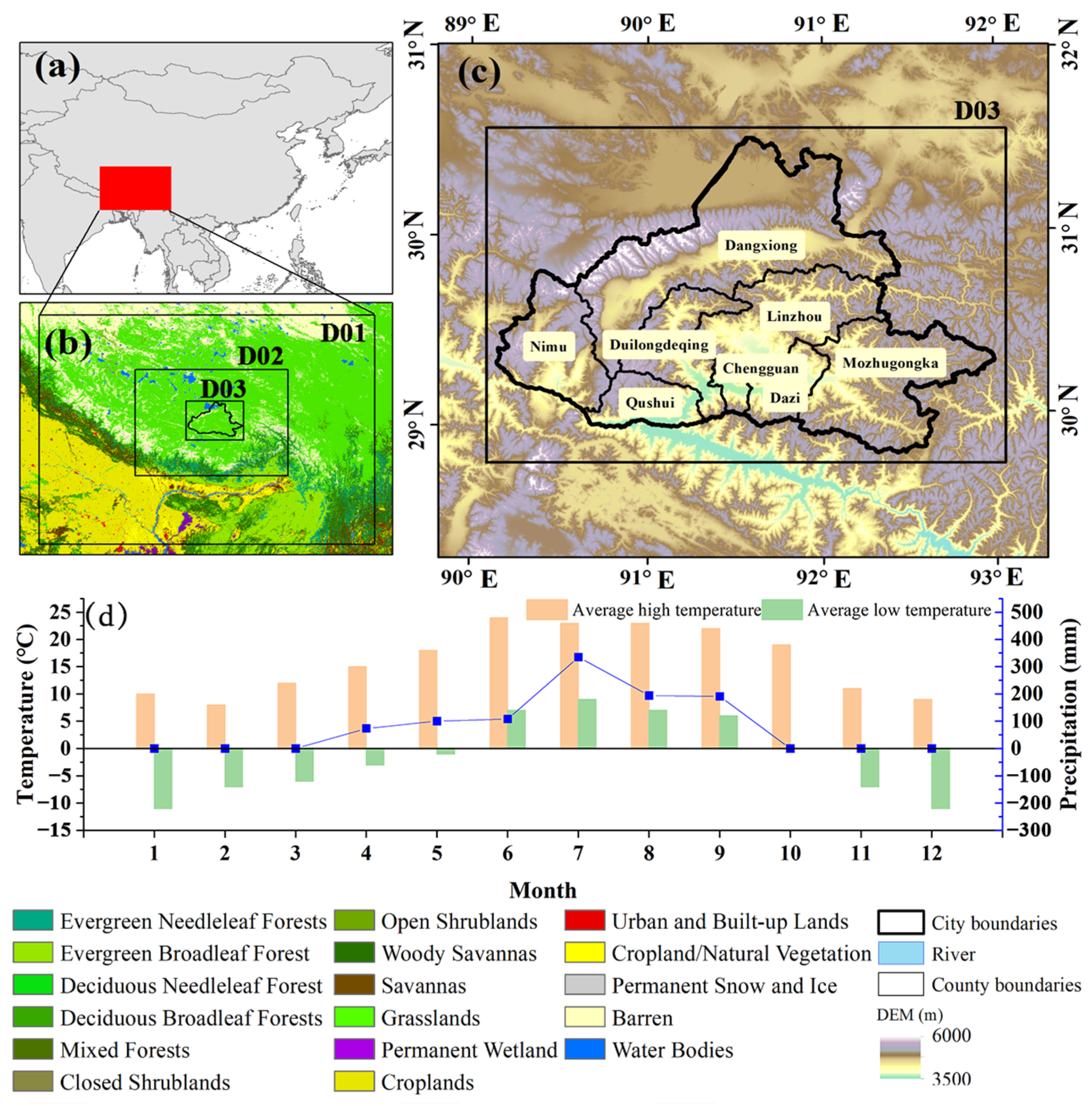
Lhasa is located in the northern part of the middle reaches of the Yarlung Tsangpo River and its tributary, the Lhasa River basin (Figure 1a). Its geographical coordinates range from 29°14′26″–31°03’45″ N to 89°45′9″–92°37′16″ E (Figure 1c). The total area is 29,528.91 km2, including Chengguan District and seven counties: Dazi, Duilongdeqing, Qushui, Linzhou, Mozhugongka, Nimu, and Dangxiong. The permanent resident population is 860,000 people. According to the vegetation zoning of Tibet, Lhasa belongs to the shrub zone of the southern Tibetan mountains, with relatively high vegetation coverage (Figure 1b). With economic development and the background of western development, Lhasa has undergone significant changes as the economic, social, and cultural center of Tibet. In 2022, the gross domestic product of the region was 74.757 billion yuan, with the value added of the primary industry at 2.674 billion yuan, the value added of the secondary industry at 29.125 billion yuan, and the value added of the tertiary industry at 42.958 billion yuan. The consumer price index for residents has been increasing year by year.
2.2. Datasets
This paper utilizes five types of data, which can be categorized into MODIS data, FNL data, and other data. The data sources for each type are listed in Table 1.
2.2.1. Modis Data
This paper utilizes two types of MODIS data. The first type of data are the LST data from MOD11A1 (daytime product), with a spatial resolution of 1 km and a temporal resolution of 1 day. It is used to provide clear-sky pixels. Temperature data are obtained from the scanning product of MOD11_L2. Relevant research indicates that the data exhibit a high level of accuracy, with an error of 2 K relative to the observed data [41]. Due to its high temporal resolution, it is commonly used in various studies related to thermal environments. The second type of data are MODIS NDVI, which is a ground-standard data product derived from MOD13Q1 data product released by the NASA Data Center in the United States. The spatial resolution of the data is 250 m, and the temporal resolution is 16 days.
2.2.2. FNL Data
FNL data are a global meteorological analysis dataset. Due to its integration from multiple data sources and quality control, it exhibits high accuracy and is widely applied in meteorological research and climate analysis [42]. In this article, we utilized the FNL ds083.2 dataset. Although the spatial resolution of the data is coarse at 1°, the data can be dynamically downscaled using the WRF model and have been commonly used as driving data for the WRF model. Additionally, the dataset exhibits a relatively high temporal resolution of 6 h, allowing for the simulation of variable values at specific time points using the WRF model based on these data.
2.2.3. Other Data
The other data in this study include DEM and LAT data. The DEM data are derived from resampled Shuttle Radar Topography Mission data based on the U.S. Space Shuttle [43]. The spatial resolution of these data is 250 m.
3. Methodology
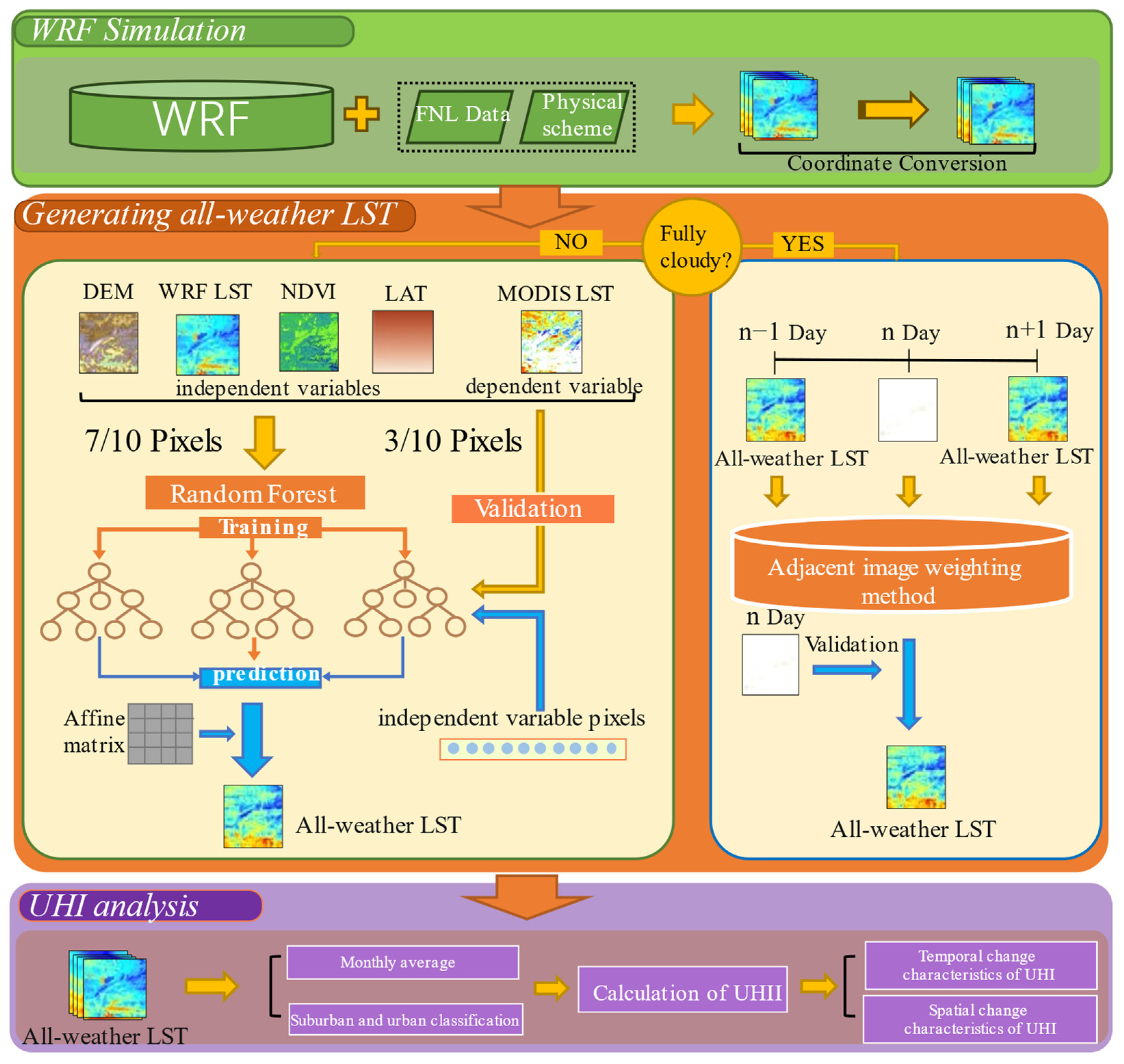
The study in this paper focuses on reconstructing the all-weather LST for March, June, September, and December 2020 in the Lhasa region and exploring UHI effects in the area using the reconstructed data. Because the daily MODIS LST data in these four months were consistently contaminated by clouds, they are suitable for validating the LST reconstruction method proposed in this paper. Additionally, these four months can individually represent the four seasons, making them applicable for conducting seasonal analysis of UHI in the study area. Therefore, these four months have been selected as the research period. The content consists of three parts (Figure 2). The first part involves using the WRF model to simulate the WRF LST source data for LST reconstruction. To ensure spatial consistency between the simulated WRF LST and MODIS LST, the coordinate system is transformed to WGS84 with a resolution of 0.01°. The second part focuses on generating the all-weather LST. Firstly, based on the physical model WRF, WRF LST is simulated. Then, by combining multisource remote sensing observation data such as NDVI, DEM, and LAT, all-weather LST is reconstructed through a Random Forest model. The final part focuses on examining the UHI effect in the study area based on the reconstructed all-weather LST. The urban heat island intensity (UHII) is analyzed to investigate the spatiotemporal distribution characteristics of the UHI. To ensure alignment with the MODIS LST data, the aforementioned five types of data underwent resampling and reprojection operations, resulting in a final spatial resolution of 0.01°, the coordinate system of WGS84 and the temporal resolution is 1 day. These operations were performed in PIE-Basic 6.0 software, which is widely used for preprocessing various sensor images and is a popular professional software option for remote sensing image processing. The LAT data are obtained by extracting latitude information of each pixel from the elevation data. The spatial and temporal resolutions of these data are the same as those of the DEM data.
3.1. All-Weather LST Reconstruction
3.1.1. WRF Configuration
The simulation results of the WRF model exhibit a downscaled spatial resolution through the use of nested configurations. In this study, a three-level nested domain configuration (Figure 1b) was selected. The domains of each level are 127 × 105, 220 × 202, and 334 × 334. They are named D01, D02, and D03, with the spatial resolution of the final level reaching 1 km. The chosen projection type is the Lambert projection, with the center of projection located at the center of Lhasa (30.126° N, 91.016° E). The latitudes of the intersection points where the projection cone and sphere are tangent are 60° and 30°, respectively. The selection of the WRF scheme can affect the accuracy of the simulation results. Based on relevant research conducted in the region [44], the following WRF physics schemes (Table 2) were selected in this study.
3.1.2. LST Reconstruction
The reconstruction method for the all-weather LST can be divided into two scenarios: the MODIS data are completely cloud-covered data and partially cloud-covered data. The reconstructed LST has a spatial resolution of 1 km and a temporal resolution of 1 day. Under the scenarios of partial cloud coverage, the MODIS LST data can be used as the training set for the RF model, with a training-to-testing pixel ratio of 7:3. Since both the testing set and the cloud-covered pixels are not involved in the training process, the accuracy of the test set pixels is assumed to be the same as that of the cloud pixels. Therefore, the accuracy of the former matches that of the latter in this study. This is the validation method for cloud-covered pixels accuracy in this paper. Under this scenario, the reconstructed LST can be obtained as follows:
where LSTREC denotes the all-weather LST, LSTWRF, DEM, and NDVI are the driving data for the RF model, and f denotes the RF model.
Under the scenarios with completely cloud-covered MODIS data, resulting in no clear-sky MODIS LST pixels available as a training set for the RF model or too few clear-sky pixels leading to a low accuracy of LST reconstruction (the reconstructed LST ρ < 0.8; ρ greater than 0.8 indicates a high correlation [2]), the reconstructed LST from temporally adjacent images can be used to obtain the reconstructed LST of the current day. Temporal adjacent images do not have to be chosen only one day apart. The selected date is the one closest to the target date, and the LST can be reconstructed using Equation (1). Accuracy verification in this situation is based on a small number of remaining pixels in the image. If all pixels are covered by clouds, the LST for the target date is subjected to accuracy verification. The weighted method based on temporal adjacent images can be expressed as:
where LSTREC denotes the all-weather LST using the weighted method of temporal adjacent images, f is the RF model using temporal adjacent images, COR is the correlation between the MODIS LST and LSTREC for the corresponding date, and ρ is the correlation between the MODIS LST and LSTcWRF for the corresponding date. When the number of clear-sky pixels in the MODIS data is 0, ρ is considered as 1. Moreover, e denotes the weight of temporal adjacent images excluding the current day, and ω denotes the weight of temporal adjacent images including the current day. T and M are the number of days between a certain adjacent day and the current day and the total number of days (4 in this study) [45], respectively.
3.1.3. Accuracy Verification Metrics
The accuracy of the reconstructed LST includes the computation of accuracy for both cloud-covered pixels and all pixels. The accuracy of cloud-covered pixels is the error between test set pixels (not involved in model training) and corresponding MODIS LST pixels, while the accuracy of all pixels is the error between reconstructed LST and all clear-sky MODIS LST pixels. Three metrics, namely, the mean absolute error (MAE), the root mean square error (RMSE), and the Pearson correlation coefficient (ρ), were utilized to validate the accuracy of the reconstructed LST data. The MAE is a measure of the average difference between the predicted values and actual observations, while the RMSE reflects the overall deviation between the predicted values and actual observations. In contrast, ρ is a measure of the linear relationship between the predicted values and actual observations.
where MAE, RMSE, and ρ are the accuracy verification metrics, N denotes the number of pixels, and xi and yi denote the values of the i-th pixel in two images.
3.2. Analysis of the UHI Effect
To quantitatively analyze the UHI effect in the study area, the UHII is adopted to represent the intensity of the UHI effect. To apply this method, it is necessary to first determine the suburban and urban areas. According to relevant research on the boundary between urban and suburban areas in Lhasa [46], this paper uses the LST of Chengguan District and Duilongdeqing as representative of urban LST, and the LST of Dazi, Linzhou, Nimu, Motuo, and Qushui as representative of suburban LST. The difference between these two values reflects the UHII in Lhasa. A value greater than 0 indicates the presence of an UHI effect, while a value less than 0 indicates a cool island effect. The UHII can be calculated as follows:
where UHII is the urban heat island intensity, LSTU denotes the average LST in the urban area, and LSTS denotes the average LST in the suburban area.
To analyze the spatial distribution characteristics of the UHI effect, in this study, we further classified the UHI effect into different levels. Currently, there are three main methods for defining the levels of the UHI effect: the equal-interval (EI) method, mean-standard deviation (MSD) method, and Moran’s I index–G coefficient (MG) method. Among them, the second method outperforms the other methods in terms of the temperature variation and spatial distribution differences [34]. By using this method to analyze the spatial distribution characteristics of the UHI in the study area, the differences in the spatial distribution of LST can be effectively presented. Therefore, in this study, the MSD method is adopted to classify the levels of the UHI effect (Table 3).
In Table 3, TS is the LST, μ is the mean of the LST, and σ is the standard deviation of the LST.
4. Results
4.1. All-Weather LST Reconstruction
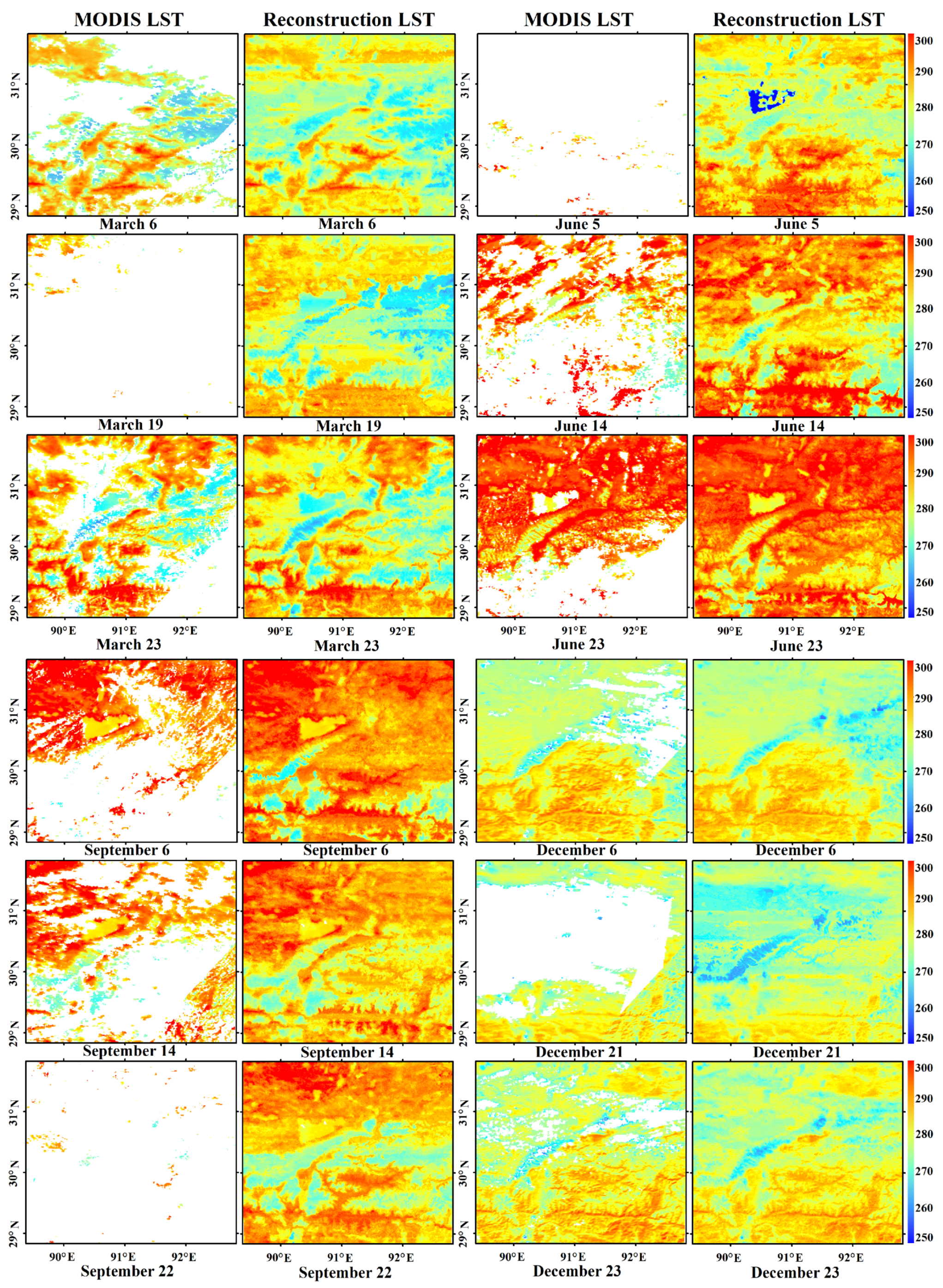
According to the abovementioned all-weather LST reconstruction method, the LST for March, June, September, and December 2020 was reconstructed. Figure 3 shows a comparison between the MODIS LST and the reconstructed LST (including pixels from the surrounding area of the study region) for these four months, with 19 March, 5 June, and 22 September as dates completely covered by clouds. It can be observed that the MODIS LST is less affected by cloud coverage in December relative to the other months, where extensive cloud coverage is observed in the MODIS LST images. The results indicate that the reconstructed LST effectively captures the spatial distribution characteristics and exhibits high spatial continuity. Moreover, many spatial details, such as the UHI effect, LST differences, and elevation temperature differences, are suitably captured in the reconstructed LST.
4.2. Accuracy of the All-Weather LST
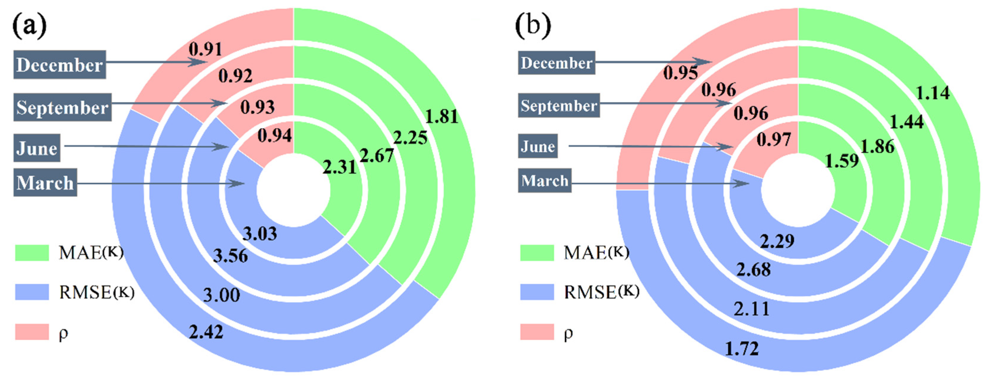
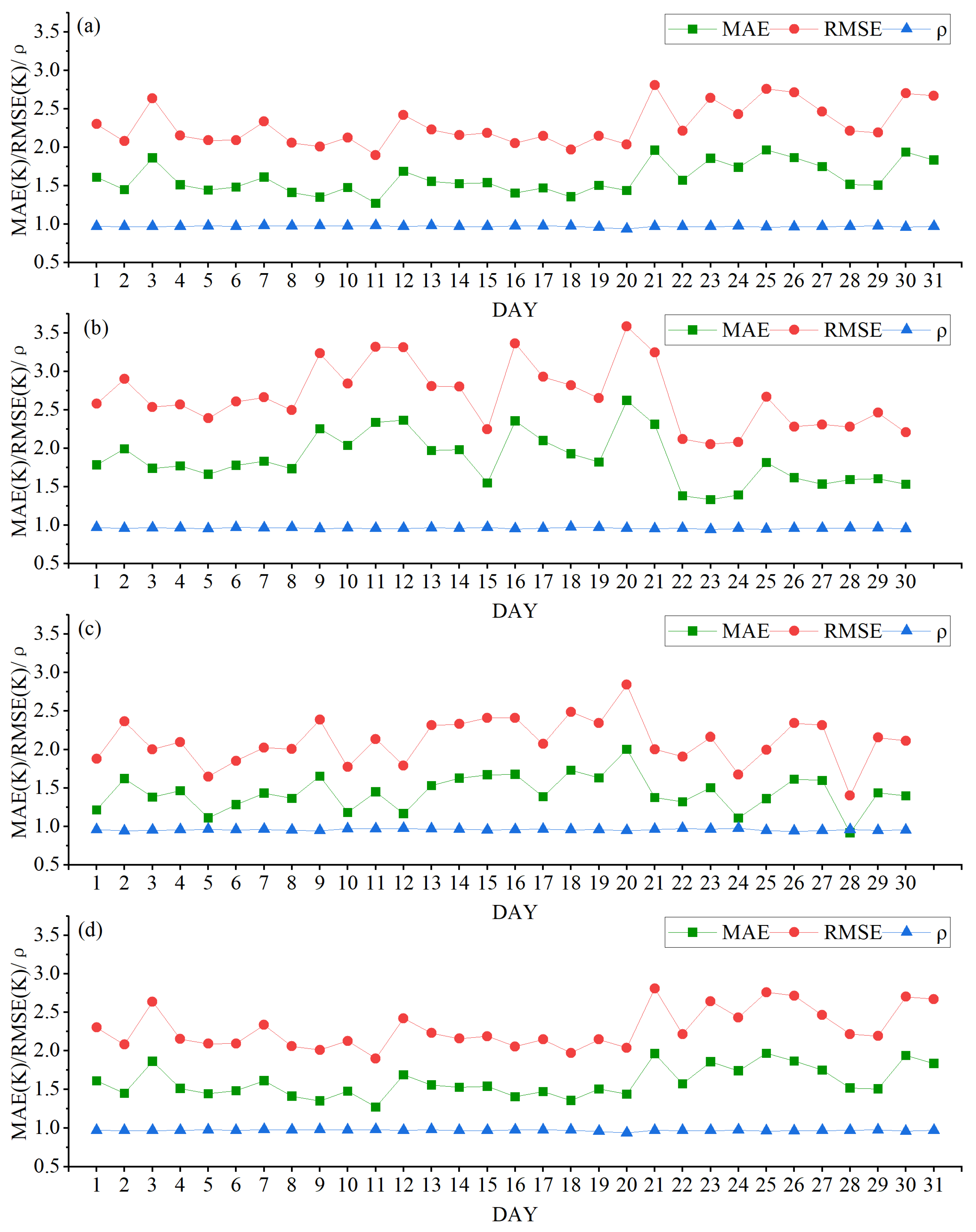
To further analyze the reliability of the reconstructed LST. First, the accuracy of cloud pixels and all pixels for these four months was calculated. Figure 4a reveals that the MAE of cloud pixels is approximately 2 K, the RMSE is approximately 3 K, and ρ consistently exceeds 0.9, indicating a high accuracy in reconstructing cloud pixels. Similarly, as shown in Figure 4b, the MAE of all pixels is approximately 1 K, the RMSE is approximately 2 K, and ρ consistently exceeds 0.9, indicating a high accuracy in reconstructing all pixels.
The average accuracy for each month is calculated above. Next, daily accuracy analysis of these four months was conducted. Figure 5 shows that the accuracy of the reconstructed LST fluctuates with the day in all 4 months. For example, the accuracy is relatively low on 21, 25, and 26 March, 15, 20, and 21 June, 9, 18, and 20 September, and 21, 25, and 30 December. This is mainly attributed to 2 factors: 1. the high cloud coverage in the MODIS LST data, which results in insufficient pixels; and 2. the use of the weighting method of temporal adjacent images to reconstruct the LST. However, the RMSE values are consistently below 3 K, the MAE ranges from 1.0 to 2.0 K, and ρ remains above 0.9 for these dates. On the other dates, the accuracy is higher, with the RMSE ranging from 1.5 to 3.0 K, and ρ still exceeding 0.9. Overall, the reconstructed LST in this study demonstrates a high level of accuracy, with an average RMSE of 2.20 K, an average MAE of 1.51 K, and a ρ value consistently above 0.9. The resulting data possesses both all-weather characteristics and high precision.
4.3. Analysis of the Urban Heat Island Intensity
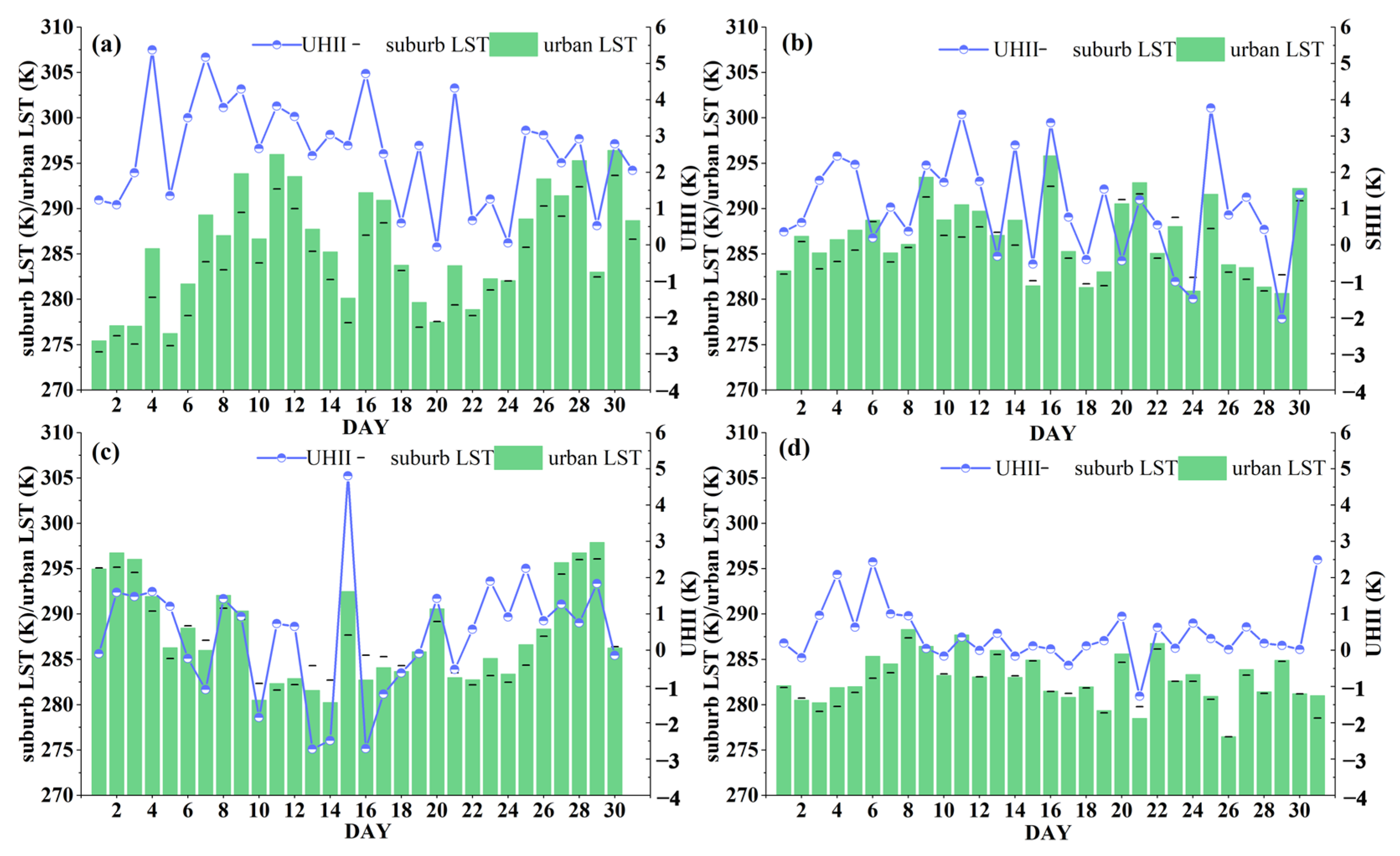
Figure 6 shows the daily UHII and LST in the urban and suburban areas for the four months. Both the UHI effect and cold island effect occurred in Lhasa in these four months. The urban LST, suburban LST, and UHII values exhibited the highest variability in March, June, and September (Figure 6a–c). The changes in the urban LST, suburban LST, and UHII values remained relatively stable in December (Figure 6d). Furthermore, March and December exhibited the largest number of days with the UHI effect, accounting for 30 days (96.77%) and 25 days (80.65%), respectively, followed by June and September, with 23 days (76.67%) and 18 days (60.00%), respectively. If we consider March, June, September, and December as the four representative months for the spring, summer, autumn, and winter seasons, respectively, the UHI effect in Lhasa mainly occurs during the spring and winter seasons, with the UHII remaining relatively stable in winter.
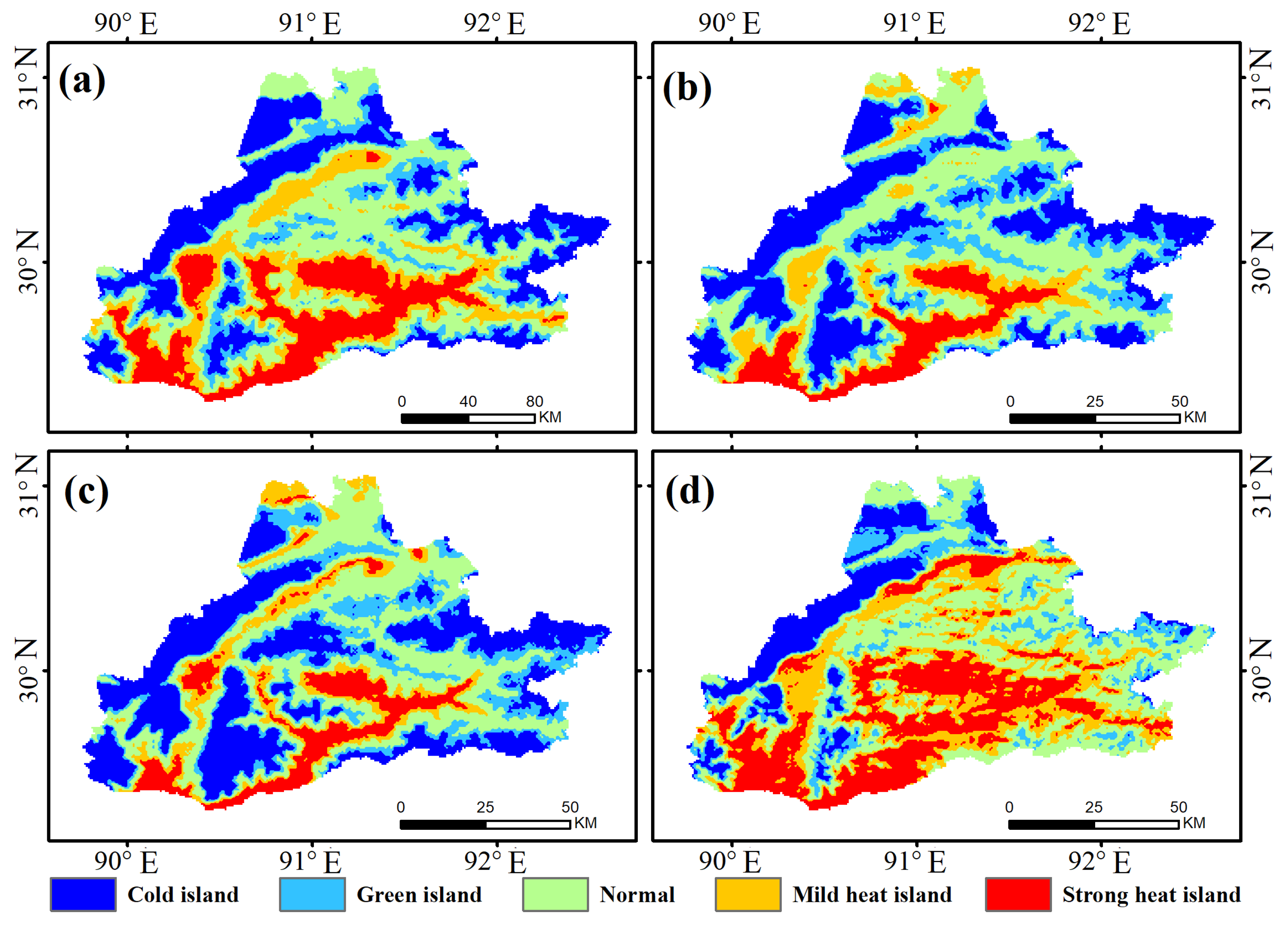
Figure 7 shows the spatial distribution of the UHI effect in the four months. In March (Figure 7a), the areas and proportions of cold islands, green islands, normal areas, mild heat islands, and strong heat islands are 6829 km2 (23.42%), 3980 km2 (13.65%), 9230 km2 (31.66%), 4251 km2 (14.58%), and 4867 km2 (16.69%), respectively. In June (Figure 7b), the areas and proportions are 8265 km2 (28.35%), 5291 km2 (18.15%), 9778 km2 (33.54%), 3036 km2 (10.41%), and 2787 km2 (9.56%), respectively. In September (Figure 7c), the areas and proportions are 9375 km2 (32.15%), 5034 km2 (17.27%), 8920 km2 (30.59%), 3059 km2 (10.49%), and 2769 km2 (9.50%), respectively. In December (Figure 7d), the areas and proportions are 3513 km2 (12.05%), 3273 km2 (11.23%), 9422 km2 (32.31%), 6170 km2 (21.16%), and 6779 km2 (23.25%), respectively. The largest heat island area is mostly observed during the spring and winter seasons, followed by the summer and autumn seasons. Additionally, the southwestern part of Lhasa and the Linzhou area in the central region show significant UHI effects. This occurs because the major urban areas of Lhasa are located along the Lhasa River, which is situated in the southwestern region, resulting in a more significant UHI effect in this area relative to the other regions.
5. Discussion
In this study, we combine the WRF model with remote sensing data to reconstruct the all-weather LST at a resolution of 0.01° while using the MODIS LST as a reference in terms of accuracy. This approach overcomes the limitation of incomplete LST retrieval from satellite TIR imagery due to the influences of clouds and precipitation. The reason for using the RF model in this paper is because it has high flexibility and stability, and uses an “averaging” approach to enhance prediction accuracy and control overfitting. It is commonly used in various LST inversion model studies [27,34,47]. The reconstructed LST in this paper exhibited a high degree of accuracy, with an average RMSE of 2.20 K, average MAE of 1.51 K, and ρ greater than 0.9. Reconstructing the all-weather LST has consistently remained a topic of interest [5,48], and several studies have been conducted. For instance, Zhou, et al. [49] proposed the data interpolating empirical orthogonal functions (DINEOF) method for LST reconstruction, with an RMSE of 4.57 K. Duan, Li and Leng [7] fused TIR and passive microwave data to reconstruct the LST, with an RMSE ranging from 3.50 to 4.40 K. Li, et al. [50] introduced a three-step mixed gap-filling method, with an RMSE of 4.78 K. Long, Yan, Bai, Zhang and Shi [9] utilized a data fusion approach combined with bias correction to reconstruct the LST, with an RMSE of 2.72 to 4.00 K. Compared with previous results [41], the reconstructed LST in this study exhibits a higher precision and hence can provide a valuable reconstruction approach for future research and serve as a fundamental data source for studies related to the thermal environment.
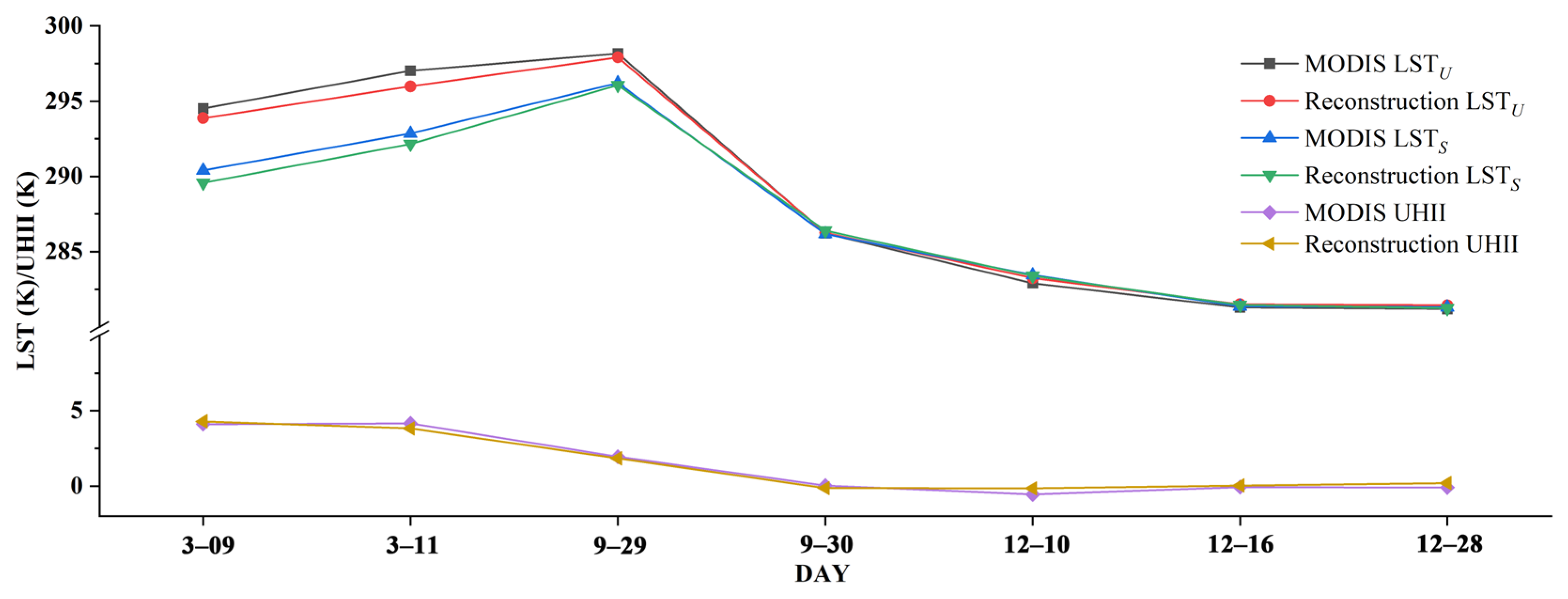
Based on the reconstructed all-weather LST, in this study, we also analyzed the UHI effect in the Lhasa region. The occurrence of the UHI effect could be better captured in March and December, indicating that the UHI effect in Lhasa can mainly be observed during the spring and winter seasons. Moreover, the UHII in winter is relatively stable, which is similar to the conclusions drawn by Ciren, Ga, Bu and Ciren [46] based on meteorological station data. Additionally, from the spatial distribution of the UHI effect in Lhasa, high-UHI areas are more prevalent during the spring and winter seasons than during the summer and autumn seasons. Furthermore, the UHI effect is primarily concentrated in the southwestern part of Lhasa and the Linzhou area in the central part. This occurs because the important urban areas of Lhasa are developed along the Lhasa River [38], which is located in the southwestern region of Lhasa, leading to a more pronounced UHI effect relative to the other regions. In recent years, the Lhasa region has experienced rapid economic development, leading to increased density of buildings. This has resulted in strong diffuse reflection and low wind speed, which hinders heat dissipation [40]. Additionally, with the growing population, artificial heat release in the main residential areas has become significant [51]. As a result, the region has exhibited noticeable HUI. The UHI in the Lhasa region reduces air density and lowers atmospheric pressure in the high-temperature areas. This leads to the continuous influx of various exhaust gases and harmful chemicals into the high-temperature zone, making residents highly susceptible to digestive or neurological disorders. To verify the reliability of the UHI results, we selected dates with minimal cloud and precipitation influences in the MODIS data, which provided a higher coverage of clear-sky pixels in both the urban and suburban areas (needed for UHII calculation). A comparison was made between the urban MODIS LST and reconstructed LST, the suburban MODIS LST and reconstructed LST, and the urban UHII and suburban UHII. The results for both datasets were highly consistent (Figure 8), indicating the high reliability of UHII analysis in this study.
As we utilized the WRF model in this study to reconstruct the all-weather LST, its application requires high computational power and a significant amount of time. Approximately three days are needed to simulate one month of data, resulting in relatively high computational costs [52]. With future advancements in computing power, it will be possible to apply the methodology proposed in this paper to reconstruct long-term LST data for various studies on thermal environments. Although the spatial distribution details of WRF LST are not sufficient and its accuracy is relatively lower compared to MODIS LST, its all-weather characteristics make it suitable for compensating for missing data from MODIS LST [13]. Since this paper is based on the reconstruction of LST from clear-sky pixels, the accuracy of cloud pixels is also validated based on clear-sky pixels. In the future, the accuracy of cloud pixels can be further improved by collecting a large amount of station data in cloud-covered areas to enhance the reliability of validating cloud pixels’ accuracy. This study only utilized some commonly used multisource remote sensing data as driving data for RF. In the future, it can be considered to incorporate more driving data that may affect LST, including water-related data, in order to further improve the accuracy of LST reconstruction. Additionally, we only conducted a simple analysis of the UHII in the research area. In future research, social and natural factors can be incorporated to analyze the driving forces behind the UHII. Thus, the impact of human activities on the UHI effect can be comprehensively explored.
6. Conclusions
In this study, we first combine WRF simulation with remote sensing data to reconstruct an all-weather LST dataset for the study area of Lhasa. This approach addresses the limitation of satellite TIR imagery, which is affected by cloud cover and precipitation, resulting in incomplete LST data. Subsequently, the reconstructed LST is analyzed to assess the UHI effect in the region. The method of reconstructing all-weather LST presented in this paper can provide new ideas for obtaining all-weather LST in the future. Although the urban heat island effect was only briefly analyzed in this study, we plan to reconstruct long-term LST in the future to further explore the thermal environment issues in the study area. The research findings are as follows:
- (1)
- The all-weather LST reconstructed in this study can effectively compensate for the missing pixels in MODIS LST and exhibits high spatiotemporal continuity. Many spatial distribution details are accurately restored. This provides a new method for the reconstruction of all-weather LST.
- (2)
- The reconstructed LST in this study demonstrates high accuracy, with an average RMSE of 2.20 K, average MAE of 1.51 K, and ρ greater than 0.9. This provides fundamental research data for studies related to the thermal environment.
- (3)
- In terms of the seasonal analysis, the UHI effect is most frequently observed during the spring and winter seasons in the Lhasa region, with the winter season showing a relatively stable UHII value. In terms of the spatial distribution, the areas with the highest proportion of strong heat islands are primarily observed during the spring and winter seasons, followed by the summer and autumn seasons.
Author Contributions
X.Z., methodology, writing, and data sources. C.M., analysis and coding. P.G., coding and investigation. Y.H., validation and investigation. Y.M., investigation and coding. W.M., data sources. Z.W., supervision. Z.H., validation. All authors have read and agreed to the published version of the manuscript.
Funding
This research was financially supported by the Second Tibetan Plateau Scientific Expedition and Research Program (Grant No. 2019QZKK0103), the National Natural Science Foundation of China (Grant Nos. 42230610, U2242208, and 41830650), and the Science and Technology Program of Zhejiang Province (Grant No. 2022C35070).
Data Availability Statement
No new data were created or analyzed in this study. Data sharing is not applicable to this article.
Conflicts of Interest
The authors declare that they have no competing interests.
References
- Wan, Z. New refinements and validation of the collection-6 MODIS land-surface temperature/emissivity product. Remote Sens. Environ. 2014, 140, 36–45. [Google Scholar] [CrossRef]
- Zhang, X.; Gou, P.; Zhang, F.; Huang, Y.; Wang, Z.; Li, G.; Xing, J. Reconstruction of all-weather land surface temperature based on a combined physical and data-driven model. Environ. Sci. Pollut. Res. 2023, 30, 78865–78878. [Google Scholar] [CrossRef] [PubMed]
- Srivastava, P.K.; Han, D.; Ramirez, M.R.; Islam, T. Machine Learning Techniques for Downscaling SMOS Satellite Soil Moisture Using MODIS Land Surface Temperature for Hydrological Application. Water Resour. Manag. 2013, 27, 3127–3144. [Google Scholar] [CrossRef]
- Zhang, F.; Zhang, X.; Chen, W.; Yang, B.; Chen, Z.; Tang, H.; Wang, Z.; Bi, P.; Yang, L.; Li, G.; et al. Cloud-Free Land Surface Temperature Reconstructions Based on MODIS Measurements and Numerical Simulations for Characterizing Surface Urban Heat Islands. IEEE J. Sel. Top. Appl. Earth Obs. Remote Sens. 2022, 15, 6882–6898. [Google Scholar] [CrossRef]
- Bartkowiak, P.; Castelli, M.; Crespi, A.; Niedrist, G.; Zanotelli, D.; Colombo, R.; Notarnicola, C. Land Surface Temperature Reconstruction Under Long-Term Cloudy-Sky Conditions at 250 m Spatial Resolution: Case Study of Vinschgau/Venosta Valley in the European Alps. IEEE J. Sel. Top. Appl. Earth Obs. Remote Sens. 2022, 15, 2037–2057. [Google Scholar] [CrossRef]
- Ding, L.; Zhou, J.; Li, Z.-L.; Ma, J.; Shi, C.; Sun, S.; Wang, Z. Reconstruction of Hourly All-Weather Land Surface Temperature by Integrating Reanalysis Data and Thermal Infrared Data From Geostationary Satellites (RTG). IEEE Trans. Geosci. Remote Sens. 2022, 60, 1–17. [Google Scholar] [CrossRef]
- Duan, S.-B.; Li, Z.-L.; Leng, P. A framework for the retrieval of all-weather land surface temperature at a high spatial resolution from polar-orbiting thermal infrared and passive microwave data. Remote Sens. Environ. 2017, 195, 107–117. [Google Scholar] [CrossRef]
- Jia, A.; Ma, H.; Liang, S.; Wang, D. Cloudy-sky land surface temperature from VIIRS and MODIS satellite data using a surface energy balance-based method. Remote Sens. Environ. 2021, 263, 112566. [Google Scholar] [CrossRef]
- Long, D.; Yan, L.; Bai, L.; Zhang, C.; Shi, C. Generation of MODIS-like land surface temperatures under all-weather conditions based on a data fusion approach. Remote Sens. Environ. 2020, 246, 111863. [Google Scholar] [CrossRef]
- Zhang, X.; Zhou, J.; Liang, S.; Wang, D. A practical reanalysis data and thermal infrared remote sensing data merging (RTM) method for reconstruction of a 1-km all-weather land surface temperature. Remote Sens. Environ. 2021, 260. [Google Scholar] [CrossRef]
- Liu, W.; Cheng, J.; Wang, Q. Estimating Hourly All-Weather Land Surface Temperature from FY-4A/AGRI Imagery Using the Surface Energy Balance Theory. IEEE Trans. Geosci. Remote Sens. 2023, 61. [Google Scholar] [CrossRef]
- Zhou, S.; Cheng, J.; Shi, J. A Physical-Based Framework for Estimating the Hourly All-Weather Land Surface Temperature by Synchronizing Geostationary Satellite Observations and Land Surface Model Simulations. IEEE Trans. Geosci. Remote Sens. 2022, 60, 112437. [Google Scholar] [CrossRef]
- Fu, P.; Xie, Y.; Weng, Q.; Myint, S.; Meacham-Hensold, K.; Bernacchi, C. A physical model-based method for retrieving urban land surface temperatures under cloudy conditions. Remote Sens. Environ. 2019, 230, 111191. [Google Scholar] [CrossRef]
- Urquhart, E.A.; Hoffman, M.J.; Murphy, R.R.; Zaitchik, B.F. Geospatial interpolation of MODIS-derived salinity and temperature in the Chesapeake Bay. Remote Sens. Environ. 2013, 135, 167–177. [Google Scholar] [CrossRef]
- Dalawi, A.N.; Lakestani, M.; Ashpazzadeh, E. Solving Fractional Optimal Control Problems Involving Caputo-Fabrizio Derivative Using Hermite Spline Functions. Iran. J. Sci. 2023, 47, 545–566. [Google Scholar] [CrossRef]
- Wenjun, Y.; Tonghua, W.; Zhuotong, N.; Lin, Z.; Zhiwei, W. A novel interpolation method for MODIS land surface temperature data on the Tibetan Plateau. Proc. SPIE 2014, 9260, 92600Y. [Google Scholar]
- Huang, C.; Duan, S.-B.; Jiang, X.-G.; Han, X.-J.; Leng, P.; Gao, M.-F.; Li, Z.-L. A physically based algorithm for retrieving land surface temperature under cloudy conditions from AMSR2 passive microwave measurements. Int. J. Remote Sens. 2019, 40, 1828–1843. [Google Scholar] [CrossRef]
- Prigent, C.; Jimenez, C.; Aires, F. Toward “all weather,” long record, and real-time land surface temperature retrievals from microwave satellite observations. J. Geophys. Res.-Atmos. 2016, 121, 5699–5717. [Google Scholar] [CrossRef]
- Reichstein, M.; Camps-Valls, G.; Stevens, B.; Jung, M.; Denzler, J.; Carvalhais, N.; Prabhat. Deep learning and process understanding for data-driven Earth system science. Nature 2019, 566, 195–204. [Google Scholar] [CrossRef]
- Jin, M.; Dickinson, R.E. A generalized algorithm for retrieving cloudy sky skin temperature from satellite thermal infrared radiances. J. Geophys. Res.-Atmos. 2000, 105, 27037–27047. [Google Scholar] [CrossRef]
- Kadaverugu, R. A comparison between WRF-simulated and observed surface meteorological variables across varying land cover and urbanization in south-central India. Earth Sci. Inform. 2023, 16, 147–163. [Google Scholar] [CrossRef]
- Zhang, X.D.; Zhou, J.; Liang, S.L.; Chai, L.N.; Wang, D.D.; Liu, J. Estimation of 1-km all-weather remotely sensed land surface temperature based on reconstructed spatial-seamless satellite passive microwave brightness temperature and thermal infrared data. Isprs J. Photogramm. Remote Sens. 2020, 167, 321–344. [Google Scholar] [CrossRef]
- Xiao, Y.; Zhao, W.; Ma, M.; Yu, W.; Fan, L.; Huang, Y.; Sun, X.; Lang, Q. An Integrated Method for the Generation of Spatio-Temporally Continuous LST Product With MODIS/Terra Observations. IEEE Trans. Geosci. Remote Sens. 2023, 61, 1–14. [Google Scholar] [CrossRef]
- Han, W.; Duan, S.-B.; Tian, H.; Lian, Y. Estimation of land surface temperature from AMSR2 microwave brightness temperature using machine learning methods. Int. J. Remote Sens. 2023, 22, 1–12. [Google Scholar] [CrossRef]
- Zhao, W.; Duan, S.-B. Reconstruction of daytime land surface temperatures under cloud-covered conditions using integrated MODIS/Terra land products and MSG geostationary satellite data. Remote Sens. Environ. 2020, 247, 111931. [Google Scholar] [CrossRef]
- Zhang, Y.; Yang, Y.; Pan, X.; Ding, Y.; Hu, J.; Dai, Y. Multiinformation Fusion Network for Mapping Gapless All-Sky Land Surface Temperature Using Thermal Infrared and Reanalysis Data. IEEE Trans. Geosci. Remote Sens. 2023, 61, 1–15. [Google Scholar] [CrossRef]
- Liu, K.; Su, H.B.; Li, X.K.; Chen, S.H. Development of a 250-m Downscaled Land Surface Temperature Data Set and Its Application to Improving Remotely Sensed Evapotranspiration Over Large Landscapes in Northern China. IEEE Trans. Geosci. Remote Sens. 2022, 60, 1–12. [Google Scholar] [CrossRef]
- Wang, S.; Fu, G. Modelling soil moisture using climate data and normalized difference vegetation index based on nine algorithms in alpine grasslands. Front. Environ. Sci. 2023, 11, 1130448. [Google Scholar] [CrossRef]
- Wang, D.; Liu, Y.; Yu, T.; Zhang, Y.; Liu, Q.; Chen, X.; Zhan, Y. A Method of Using WRF-Simulated Surface Temperature to Estimate Daily Evapotranspiration. J. Appl. Meteorol. Climatol. 2020, 59, 901–914. [Google Scholar] [CrossRef]
- Diaz, L.R.; Santos, D.C.; Käfer, P.S.; Rocha, N.S.d.; Costa, S.T.L.d.; Kaiser, E.A.; Rolim, S.B.A. Land Surface Temperature Retrieval Using High-Resolution Vertical Profiles Simulated by WRF Model. Atmosphere 2021, 12, 1436. [Google Scholar] [CrossRef]
- Leng, P.; Yang, Z.; Yan, Q.-Y.; Shang, G.-F.; Zhang, X.; Han, X.-J.; Li, Z.-L. A framework for estimating all-weather fine resolution soil moisture from the integration of physics-based and machine learning-based algorithms. Comput. Electron. Agric. 2023, 206, 107673. [Google Scholar] [CrossRef]
- Liu, Z.H.; Zhan, W.F.; Lai, J.M.; Hong, F.L.; Quan, J.L.; Bechtel, B.; Huang, F.; Zou, Z.X. Balancing prediction accuracy and generalization ability: A hybrid framework for modelling the annual dynamics of satellite-derived land surface temperatures. Isprs J. Photogramm. Remote Sens. 2019, 151, 189–206. [Google Scholar] [CrossRef]
- Yu, L.X.; Liu, Y.; Yang, J.C.; Liu, T.X.; Bu, K.; Li, G.S.; Jiao, Y.; Zhang, S.W. Asymmetric daytime and nighttime surface temperature feedback induced by crop greening across Northeast China. Agric. For. Meteorol. 2022, 325, 109136. [Google Scholar] [CrossRef]
- Lu, Y.S.; He, T.; Xu, X.L.; Qiao, Z. Investigation the Robustness of Standard Classification Methods for Defining Urban Heat Islands. IEEE J. Sel. Top. Appl. Earth Obs. Remote Sens. 2021, 14, 11386–11394. [Google Scholar] [CrossRef]
- Sheng, L.; Tang, X.L.; You, H.Y.; Gu, Q.; Hu, H. Comparison of the urban heat island intensity quantified by using air temperature and Landsat land surface temperature in Hangzhou, China. Ecol. Indic. 2017, 72, 738–746. [Google Scholar] [CrossRef]
- Lin, L.; Meng, L.N.; Mei, Y.D.; Zhang, W.T.; Liu, H.; Xiang, W.L. Spatial-temporal patterns of summer urban islands and their economic implications in Beijing. Environ. Sci. Pollut. Res. 2022, 29, 33361–33371. [Google Scholar] [CrossRef] [PubMed]
- de Speville, C.D.; Seviour, W.J.M.; Lo, Y.T.E. Predicting future UK nighttime urban heat islands using observed short-term variability and regional climate projections. Environ. Res. Lett. 2023, 18, 104044. [Google Scholar] [CrossRef]
- Zhong, Y.L.; Chen, S.Q.; Mo, H.H.; Wang, W.W.; Yu, P.F.; Wang, X.M.; Chuduo, N.; Ba, B. Contribution of urban expansion to surface warming in high-altitude cities of the Tibetan Plateau. Clim. Change 2022, 175, 1–22. [Google Scholar] [CrossRef]
- Zhong, Y.L.; Yu, H.; Wang, W.W.; Yu, P.F. Impacts of future urbanization and rooftop photovoltaics on the surface meteorology and energy balance of Lhasa, China. Urban Clim. 2023, 51, 101668. [Google Scholar] [CrossRef]
- Wang, S.; Tan, X.; Fan, F. Changes in Impervious Surfaces in Lhasa City, a Historical City on the Qinghai-Tibet Plateau. Sustainability 2023, 15, 5510. [Google Scholar] [CrossRef]
- Zhang, X.; Chen, W.; Chen, Z.; Yang, F.; Meng, C.; Gou, P.; Zhang, F.; Feng, J.; Li, G.; Wang, Z. Construction of cloud-free MODIS-like land surface temperatures coupled with a regional weather research and forecasting (WRF) model. Atmos. Environ. 2022, 283, 119190. [Google Scholar] [CrossRef]
- Huang, D.; Gao, S. Impact of different reanalysis data on WRF dynamical downscaling over China. Atmos. Res. 2018, 200, 25–35. [Google Scholar] [CrossRef]
- O’Loughlin, F.E.; Paiva, R.C.D.; Durand, M.; Alsdorf, D.E.; Bates, P.D. A multi-sensor approach towards a global vegetation corrected SRTM DEM product. Remote Sens. Environ. 2016, 182, 49–59. [Google Scholar] [CrossRef]
- Liu, L.; Zhang, X.; Han, C.; Ma, Y. A performance evaluation of various physics schemes on the predictions of precipitation and temperature over the Tibet Autonomous Region of China. Atmos. Res. 2023, 292, 106878. [Google Scholar] [CrossRef]
- Quan, J.; Chen, Y.; Zhan, W.; Wang, J.; Voogt, J.; Li, J. A hybrid method combining neighborhood information from satellite data with modeled diurnal temperature cycles over consecutive days. Remote Sens. Environ. 2014, 155, 257–274. [Google Scholar] [CrossRef]
- Ciren, L.; Ga, Z.; Bu, L.; Ciren, P. Temporal and Spatial Distribution of Urban Heat Islands Around Lhasa City. Resour. Sci. 2012, 34, 2364–2373. [Google Scholar]
- Hutengs, C.; Vohland, M. Downscaling land surface temperatures at regional scales with random forest regression. Remote Sens. Environ. 2016, 178, 127–141. [Google Scholar] [CrossRef]
- Duan, S.B.; Lian, Y.H.; Zhao, E.Y.; Chen, H.; Han, W.J.; Wu, Z.H. A Novel Approach to All-Weather LST Estimation Using XGBoost Model and Multisource Data. IEEE Trans. Geosci. Remote Sens. 2023, 61, 1–14. [Google Scholar] [CrossRef]
- Zhou, W.; Peng, B.; Shi, J. Reconstructing spatial-temporal continuous MODIS land surface temperature using the DINEOF method. J. Appl. Remote Sens. 2017, 11, 046016. [Google Scholar] [CrossRef]
- Li, X.; Zhou, Y.; Asrar, G.R.; Zhu, Z. Creating a seamless 1km resolution daily land surface temperature dataset for urban and surrounding areas in the conterminous United States. Remote Sens. Environ. 2018, 206, 84–97. [Google Scholar] [CrossRef]
- Wang, M.; Shen, P. Investigation of Indoor Asymmetric Thermal Radiation in Tibet Plateau: Case Study of a Typical Office Building. Buildings 2022, 12, 129. [Google Scholar] [CrossRef]
- Zou, H.B.; Wu, S.S.; Shan, J.S. Sensitivity of Lake-Effect Convection to the Lake Surface Temperature over Poyang Lake in China. J. Meteorol. Res. 2022, 36, 342–359. [Google Scholar] [CrossRef]
Figure 1.
Location (a), land use types (b), and administrative boundaries (c) of the study area. D01, D02, and D03 are the three nested domains in the WRF model. The land use and DEM in (b) and (c) are sourced from the Resource and Environment Science Data Center. The climate data in (d) is sourced from the China Weather Network.

Figure 2.
Technical flowchart.

Figure 3.
Spatial distribution comparison between the all-weather LST reconstructed and MODIS LST in the Lhasa region in 2020.
Figure 3.
Spatial distribution comparison between the all-weather LST reconstructed and MODIS LST in the Lhasa region in 2020.

Figure 4.
Accuracy statistics of cloud pixels (a) and all pixels (b) for the all-weather LST reconstructed in the Lhasa region in 2020.
Figure 4.
Accuracy statistics of cloud pixels (a) and all pixels (b) for the all-weather LST reconstructed in the Lhasa region in 2020.

Figure 5.
Accuracy of daily reconstructed LST in the Lhasa region for the months of March (a), June (b), September (c), and December (d) in 2020.
Figure 5.
Accuracy of daily reconstructed LST in the Lhasa region for the months of March (a), June (b), September (c), and December (d) in 2020.

Figure 6.
Values of daily urban LST, suburban LST, and UHII in the Lhasa region for the months of March (a), June (b), September (c), and December (d) in 2020.
Figure 6.
Values of daily urban LST, suburban LST, and UHII in the Lhasa region for the months of March (a), June (b), September (c), and December (d) in 2020.

Figure 7.
Spatial distribution of the UHI effect in the Lhasa area in March (a), June (b), September (c), and December (d) in 2020.
Figure 7.
Spatial distribution of the UHI effect in the Lhasa area in March (a), June (b), September (c), and December (d) in 2020.

Figure 8.
Comparison of the UHI effect between the MODIS LST and reconstructed LST.


Table 1.
Information on data sources.
| Name | Source | Time period |
|---|---|---|
| MODIS LST | MODIS data website (https://ladsweb.modaps.eosdis.nasa.gov/, accessed on 8 June 2023) | March, June, September, and December of 2020 |
| FNL | National Centers for Environmental Prediction (https://rda.ucar.edu/, accessed on 8 June 2023) | |
| DEM | Resource and Environment Science Data Center (https://www.resdc.cn/, accessed on 8 June 2023) | |
| LAT | Based on DEM data | |
| NDVI | MODIS data website (https://ladsweb.modaps.eosdis.nasa.gov/, accessed on 8 June 2023) |
Table 2.
Parameter configuration for the WRF physics schemes.
| Option Name | Parameterization | ID |
|---|---|---|
| Cumulus | Kain–Fritsch | 3 |
| Planetary Boundary layer | Mellor–Yamada–Janjic | 2 |
| Longwave Radiation | RRTMG | 4 |
| Shortwave Radiation | RRTMG | 4 |
| Surface Layer | Mellor–Yamada–Janjic | 2 |
| Microphysics | New Thompson | 8 |
| Land Surface | Noah-MP | 4 |
Table 3.
Classification method for UHI levels.
| Heat Island Intensity | Temperature Range | Temperature Range |
|---|---|---|
| Cold island | Low | TS < μ − σ |
| Green island | Medium low | μ − σ ≤ TS < μ − 0.5σ |
| Normal | Medium | μ − 0.5σ ≤ TS ≤ μ + 0.5σ |
| Subheat island | Medium high | μ + 0.5σ < TS ≤ μ + σ |
| Strong heat island | High | TS > μ + σ |
| Cold island | Low | TS < μ − σ |
| Green island | Medium low | μ − σ ≤ TS < μ − 0.5σ |
Disclaimer/Publisher’s Note: The statements, opinions and data contained in all publications are solely those of the individual author(s) and contributor(s) and not of MDPI and/or the editor(s). MDPI and/or the editor(s) disclaim responsibility for any injury to people or property resulting from any ideas, methods, instructions or products referred to in the content. |
© 2024 by the authors. Licensee MDPI, Basel, Switzerland. This article is an open access article distributed under the terms and conditions of the Creative Commons Attribution (CC BY) license (https://creativecommons.org/licenses/by/4.0/).
Share and Cite
MDPI and ACS Style
Zhang, X.; Meng, C.; Gou, P.; Huang, Y.; Ma, Y.; Ma, W.; Wang, Z.; Hu, Z. Evaluating the Reconstructed All-Weather Land Surface Temperature for Urban Heat Island Analysis. Remote Sens. 2024, 16, 373. https://doi.org/10.3390/rs16020373
AMA Style
Zhang X, Meng C, Gou P, Huang Y, Ma Y, Ma W, Wang Z, Hu Z. Evaluating the Reconstructed All-Weather Land Surface Temperature for Urban Heat Island Analysis. Remote Sensing. 2024; 16(2):373. https://doi.org/10.3390/rs16020373
Chicago/Turabian StyleZhang, Xuepeng, Chunchun Meng, Peng Gou, Yingshuang Huang, Yaoming Ma, Weiqiang Ma, Zhe Wang, and Zhiheng Hu. 2024. "Evaluating the Reconstructed All-Weather Land Surface Temperature for Urban Heat Island Analysis" Remote Sensing 16, no. 2: 373. https://doi.org/10.3390/rs16020373
Note that from the first issue of 2016, this journal uses article numbers instead of page numbers. See further details here.