
The Prediction of Cross-Regional Landslide Susceptibility Based on Pixel Transfer Learning

 , , ,
, , ,
Abstract
:1. Introduction
2. Materials
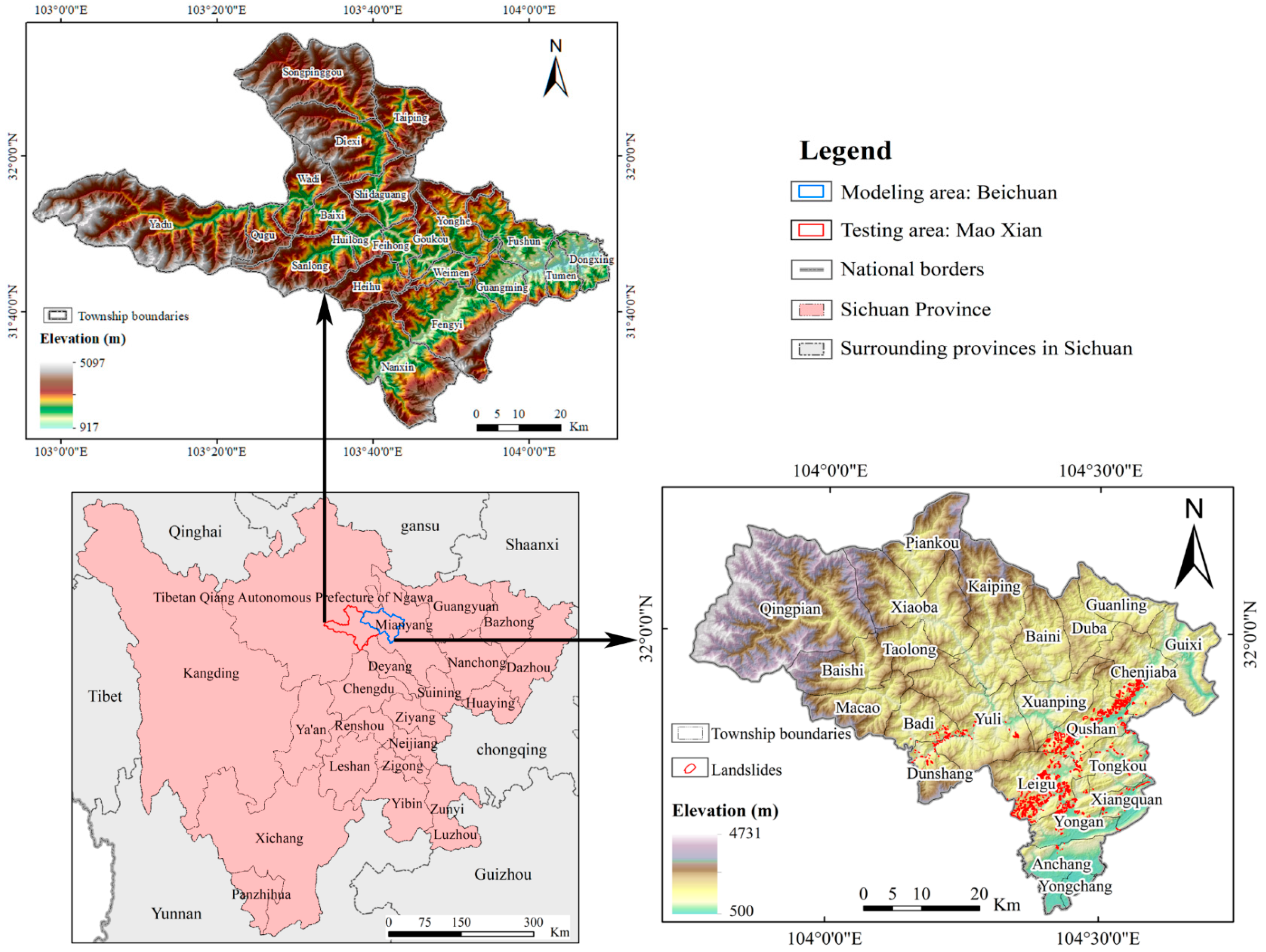
2.1. Study Area
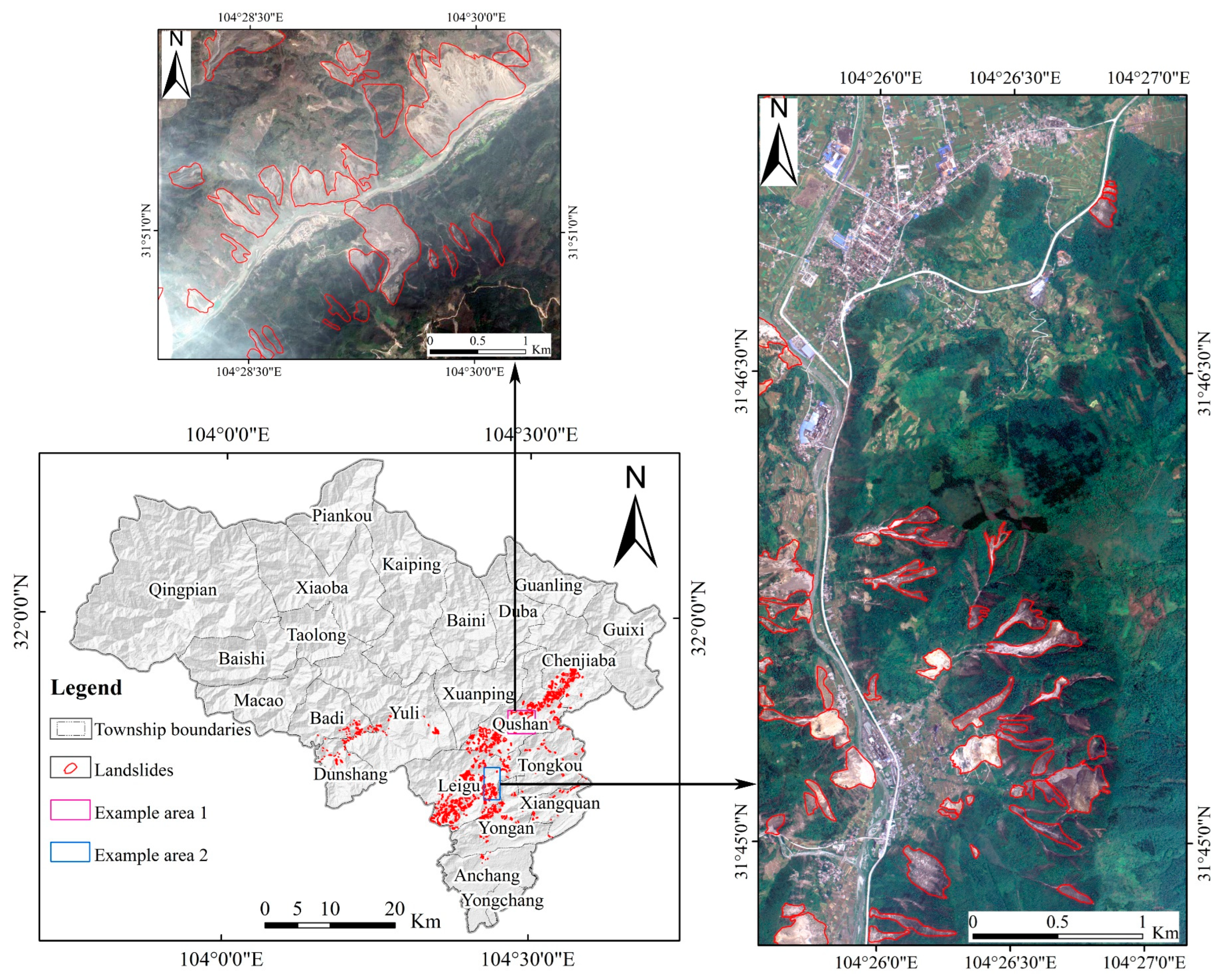
2.2. Data Collection
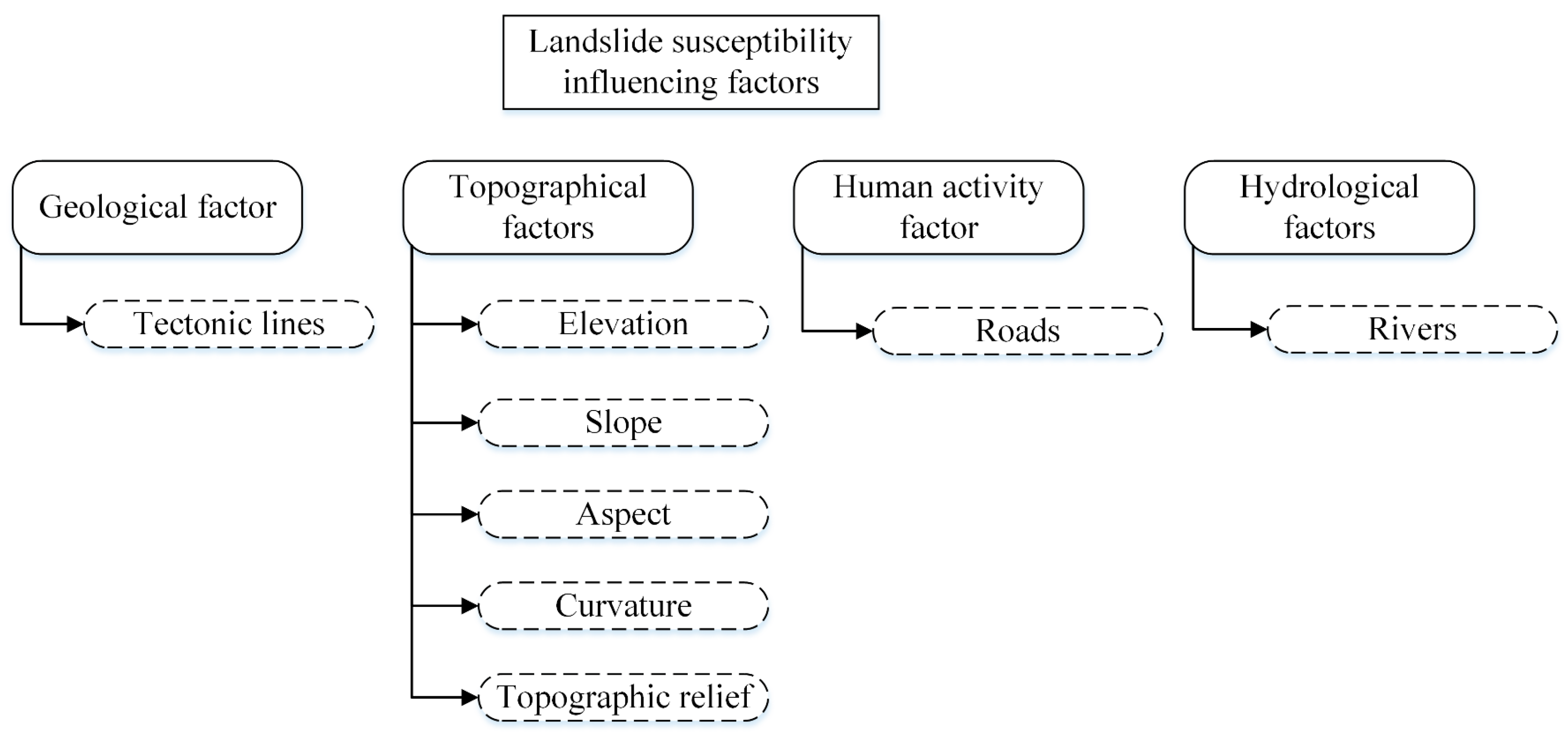
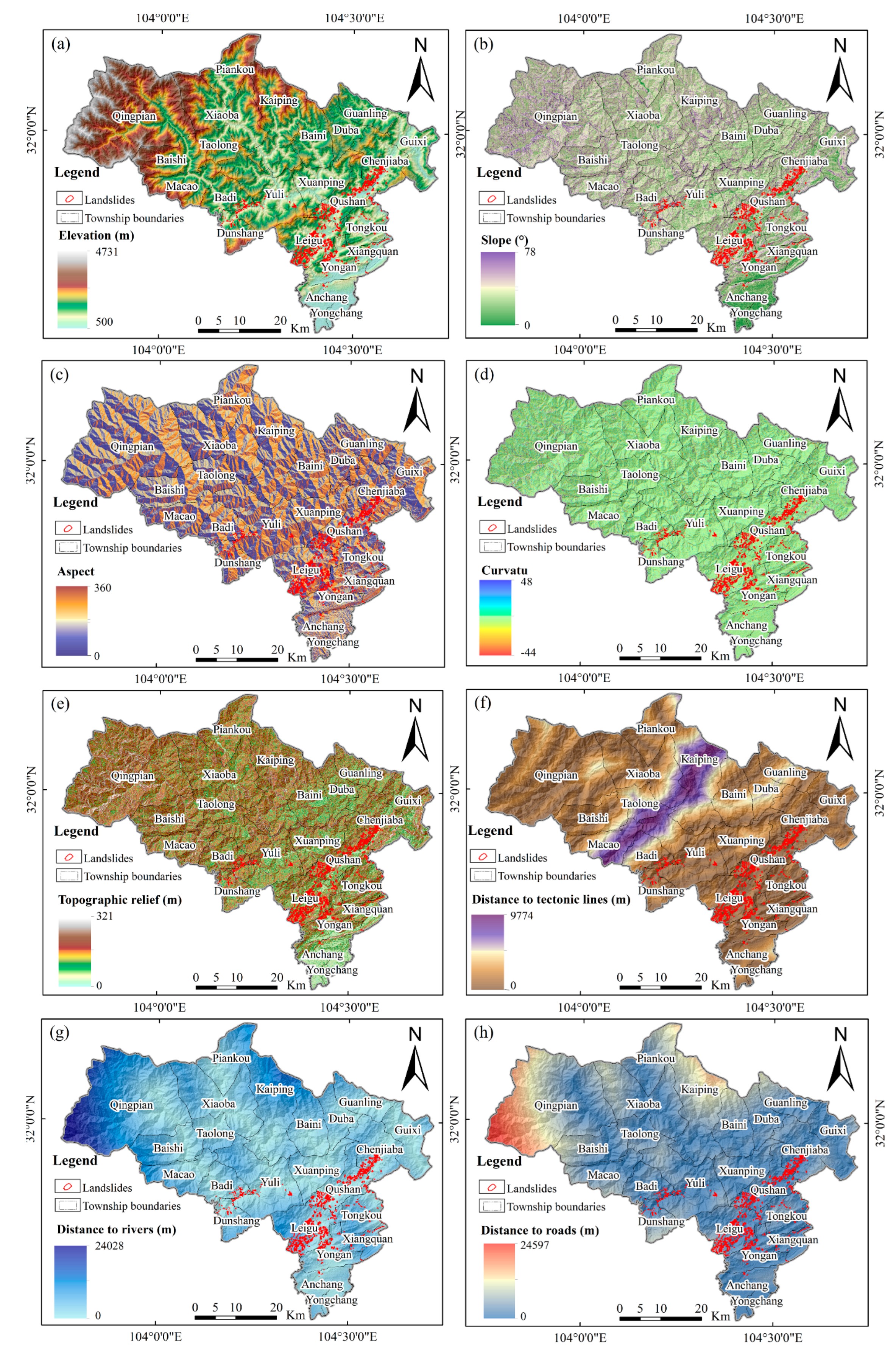
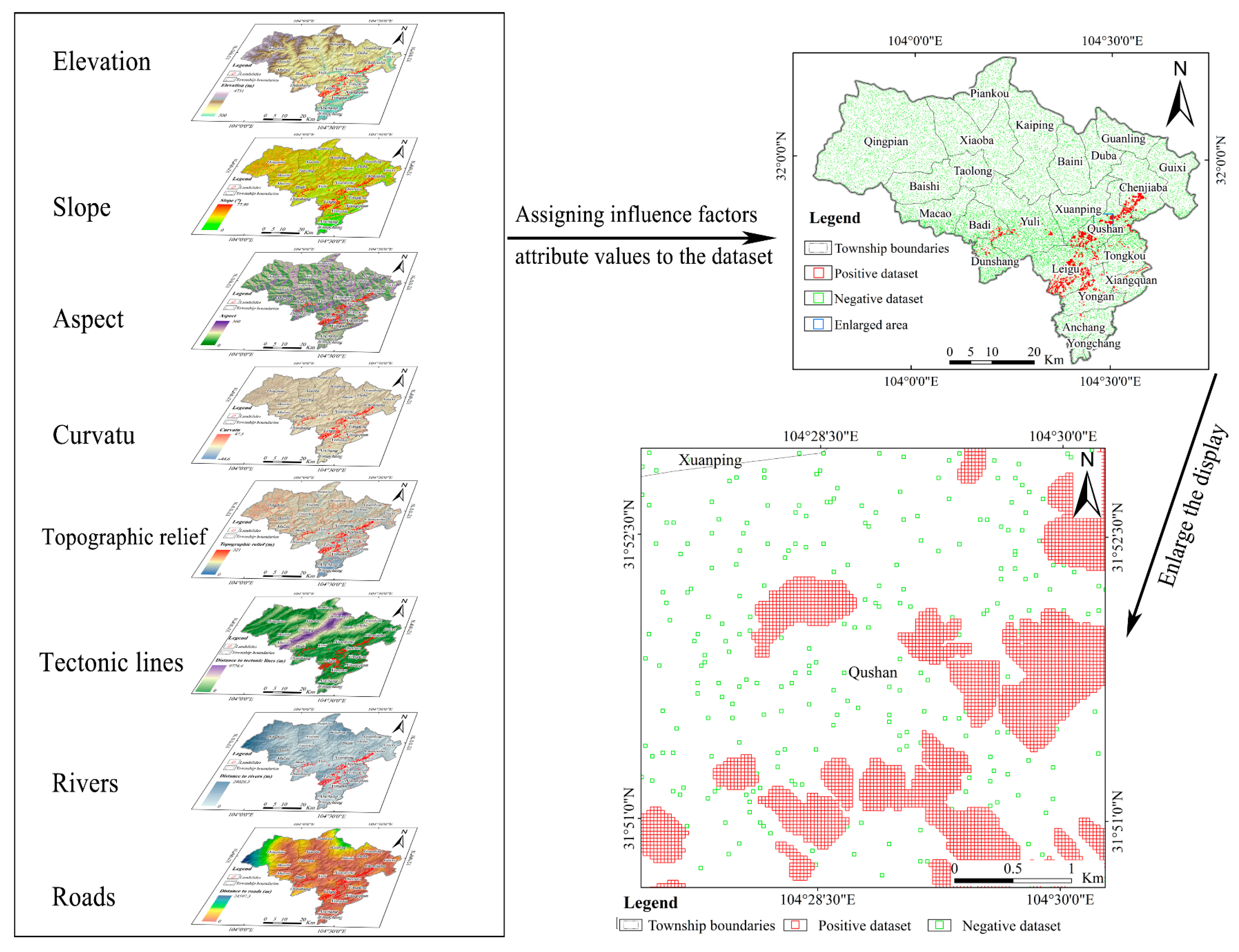
2.3. Influencing Factors
3. Methodology
3.1. Dataset Establishment
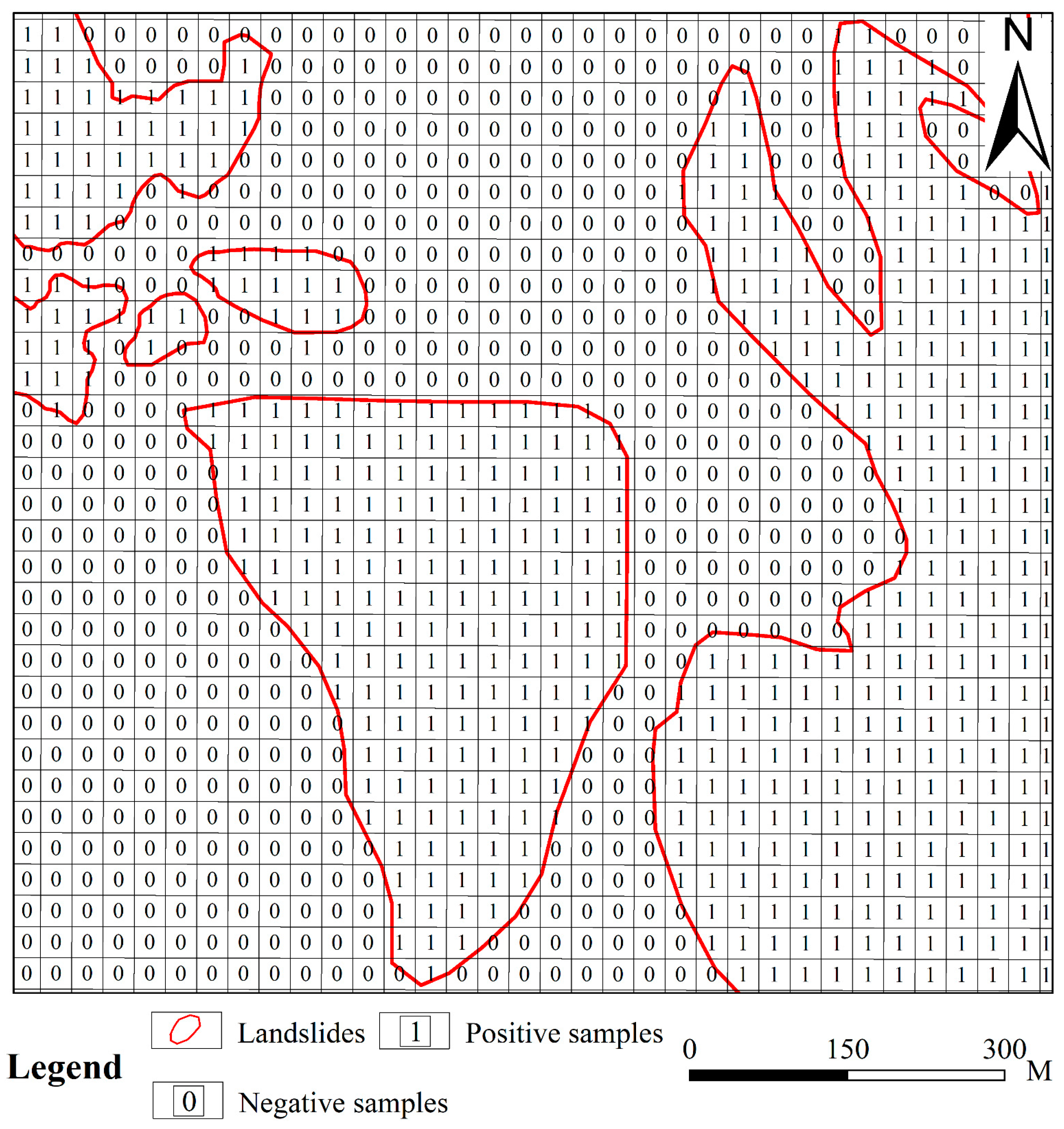
3.1.1. Mapping Unit for Susceptibility Modeling
3.1.2. Construction of the Dataset
3.2. Modeling Methods
3.2.1. Support Vector Machine (SVM)
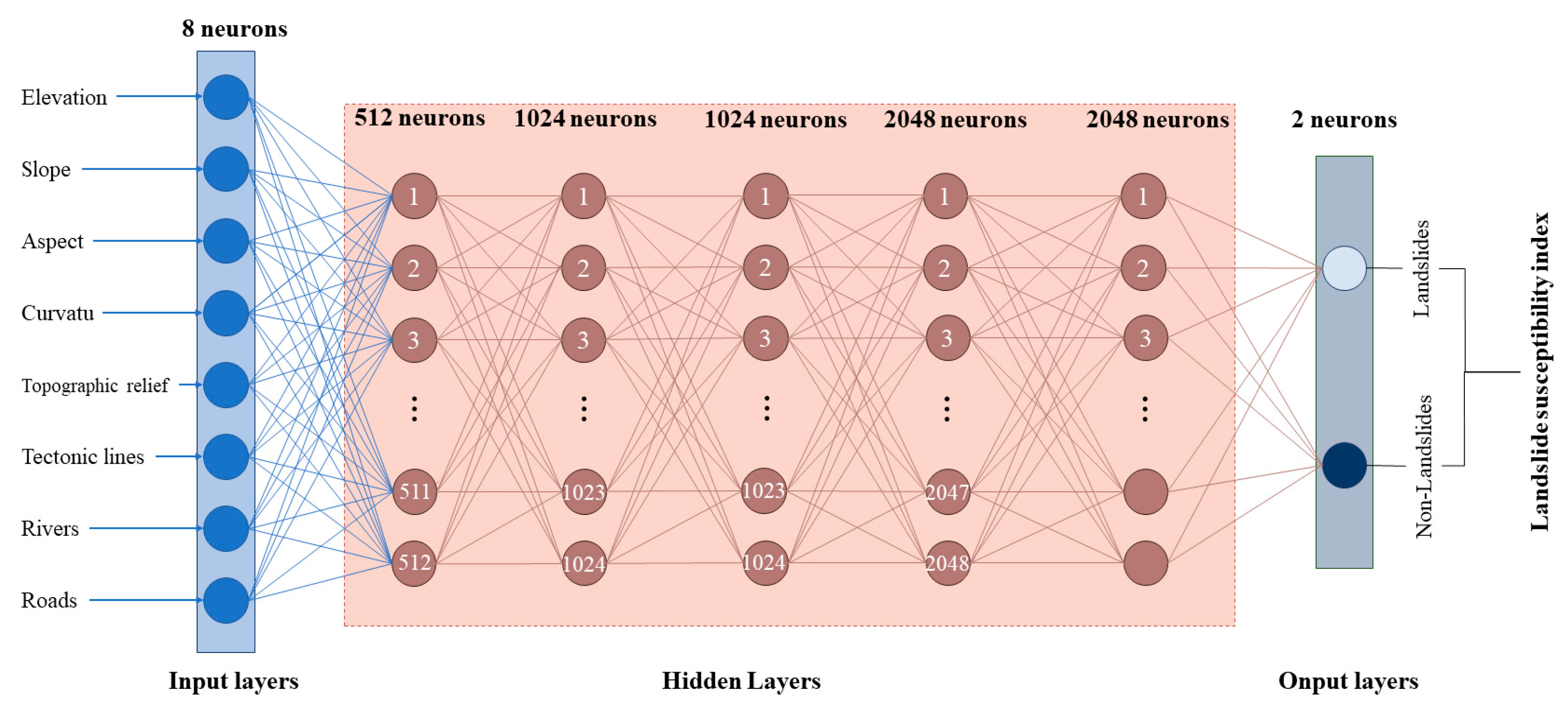
3.2.2. Deep Neural Network (DNN)
3.3. Evaluation of Model Accuracy
3.4. Transfer Learning Theory
- I.
- Inductive transfer: the source and target share the same domain, but different tasks; the source can be labeled or not, and the target needs to be labeled.
- II.
- Transductive transfer: the source and target have different but related domains and the same task; the source is labeled, and the target is unlabeled.
- III.
- Unsupervised transfer: the source and target have different domains and tasks, usually for clustering, dimensionality reduction, density estimation, etc.
4. Results
4.1. Covariance Diagnosis
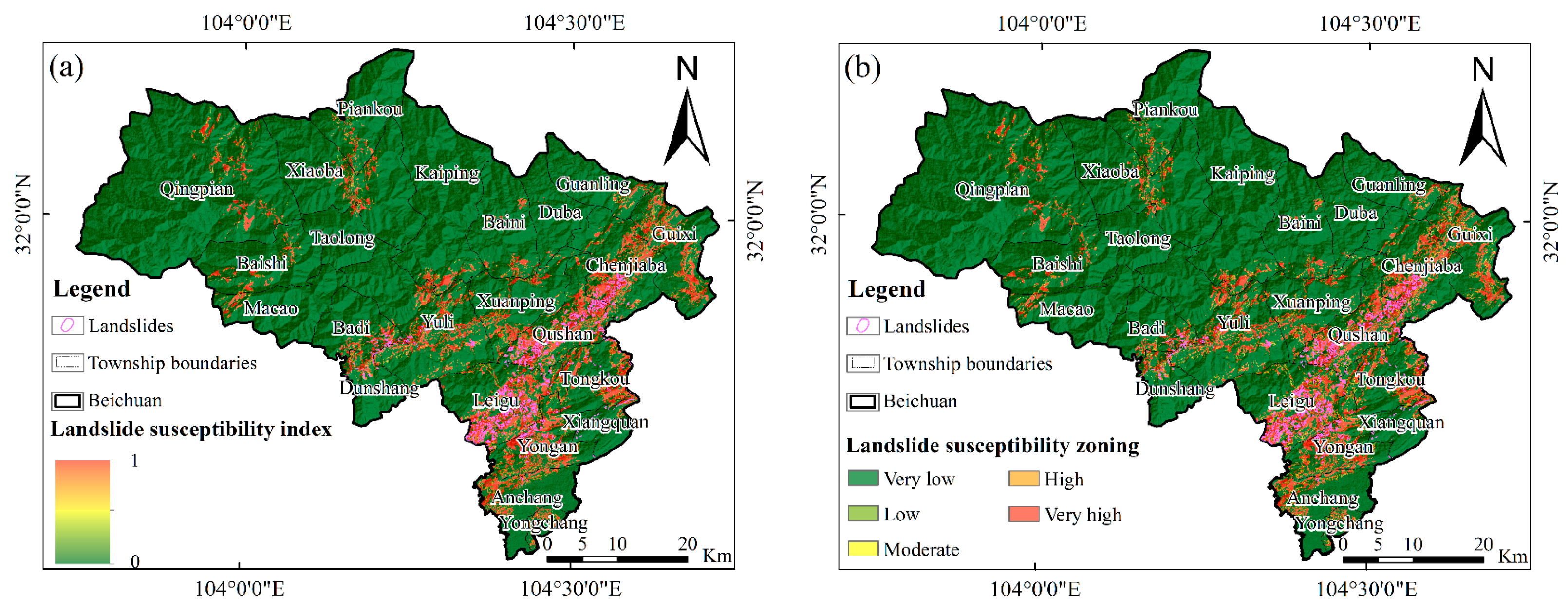
4.2. Application of the SVM and DNN Models
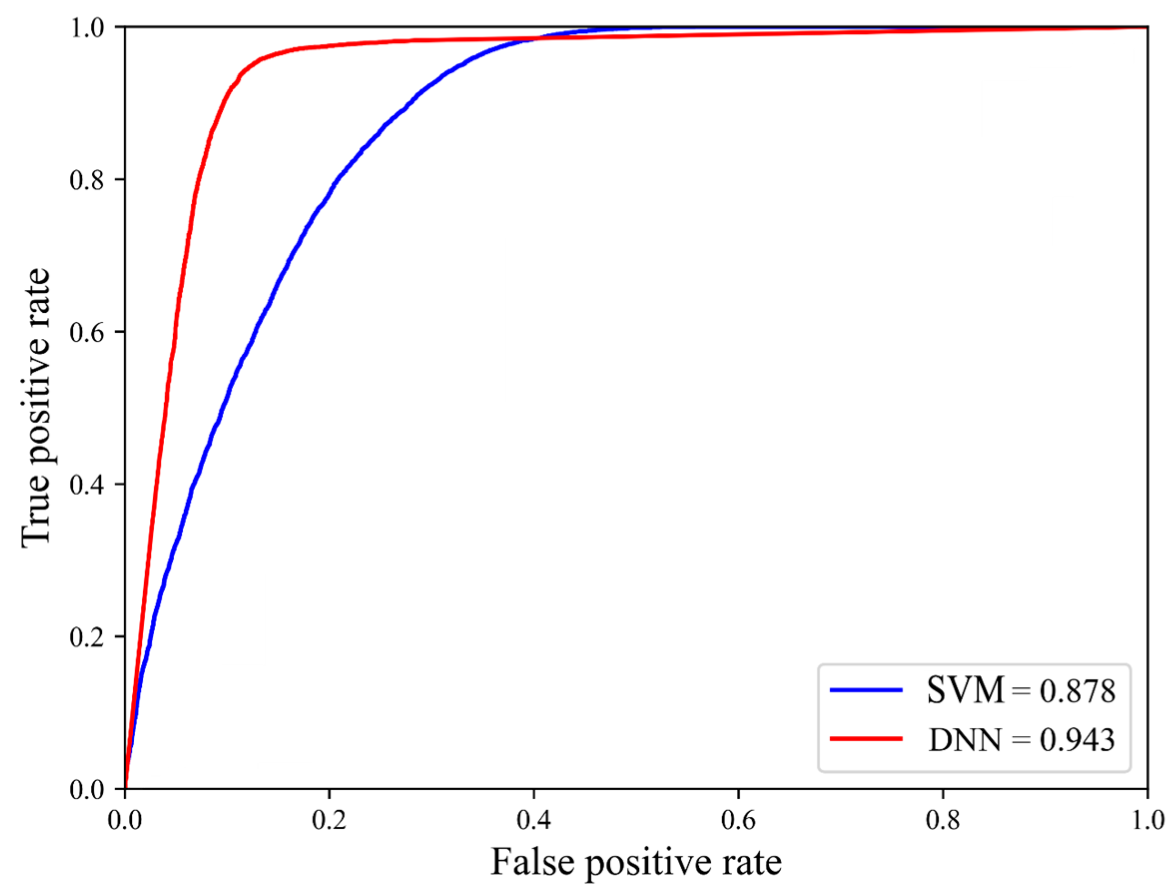
4.3. Validation of Models
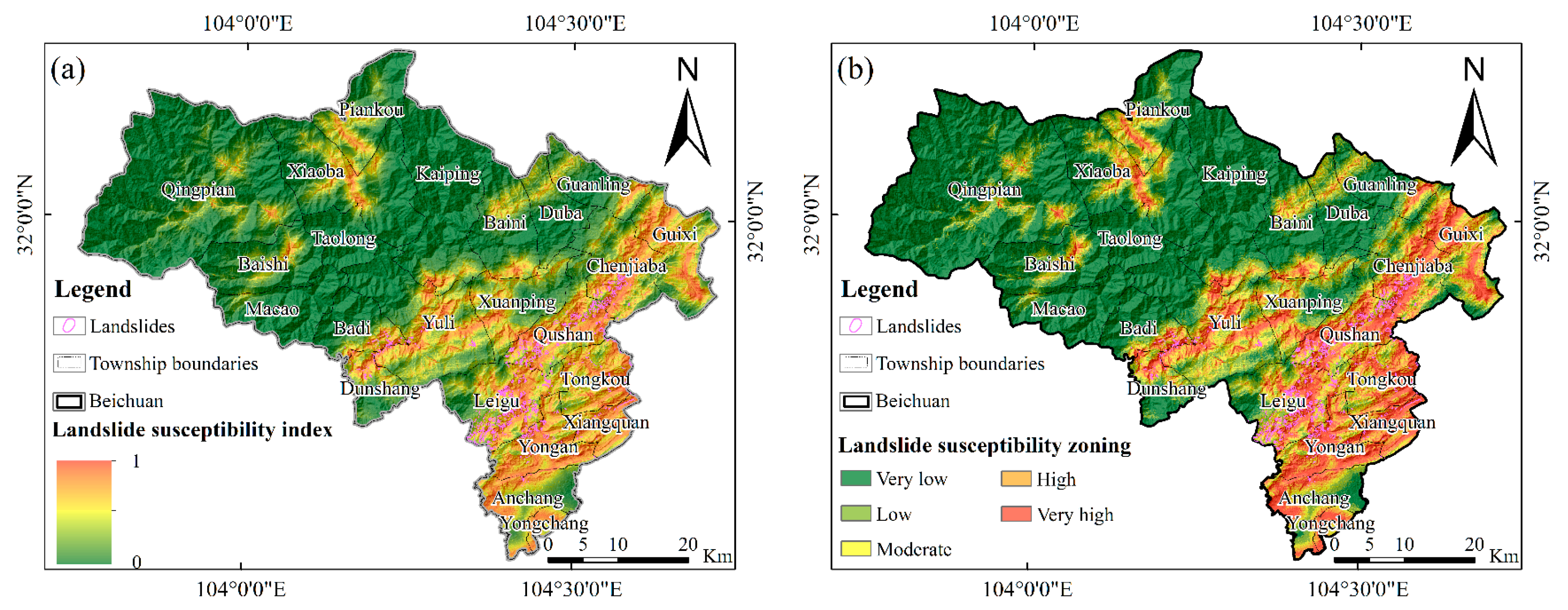
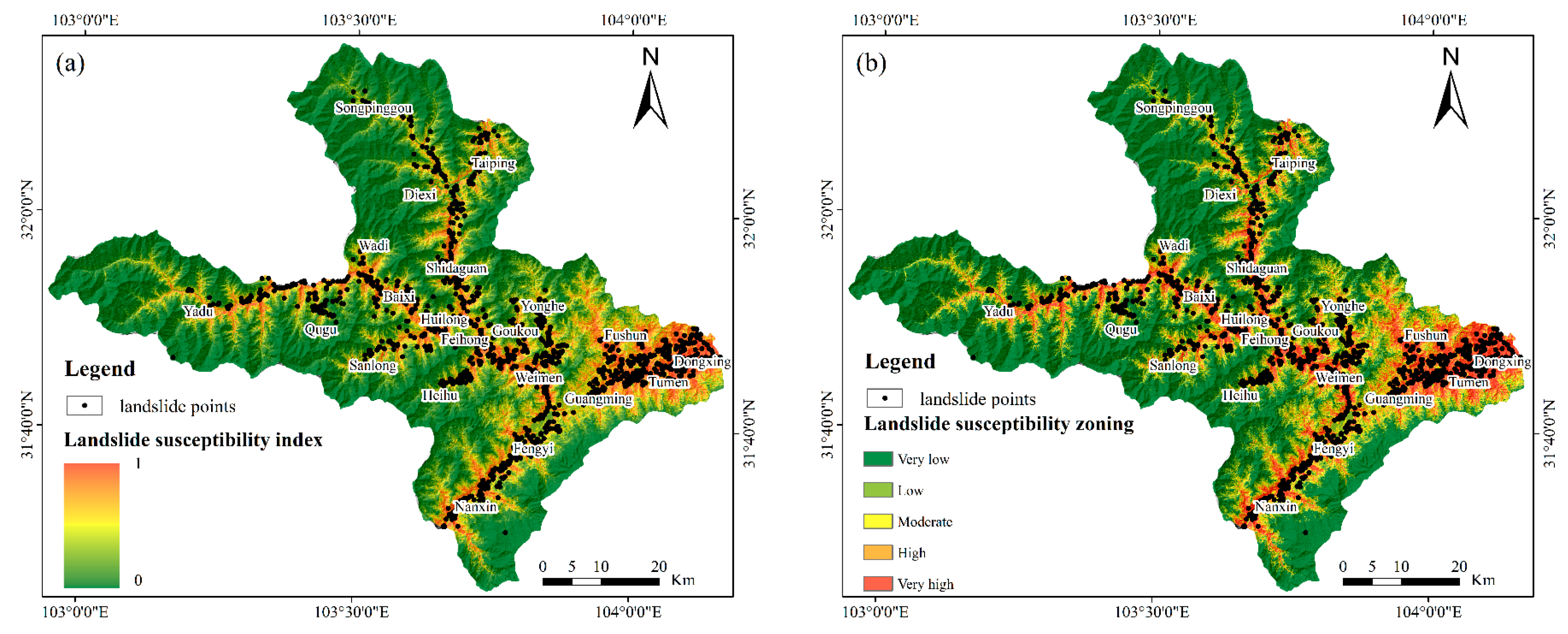
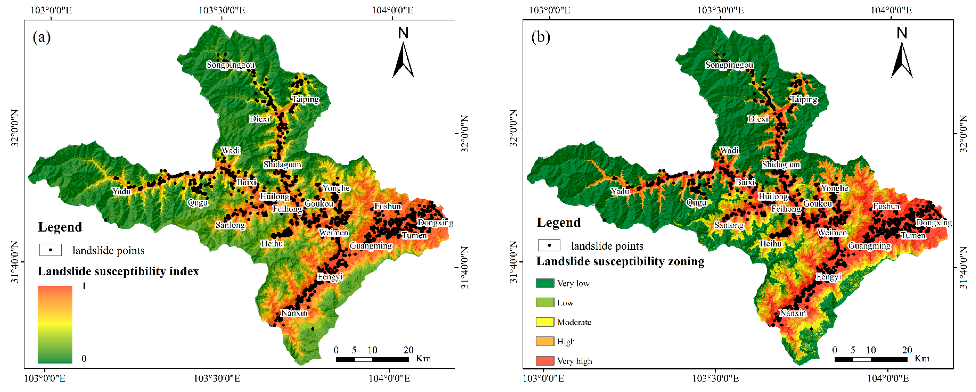
4.4. Prediction of Landslide Susceptibility in Mao County Based on Transfer Learning
5. Discussions
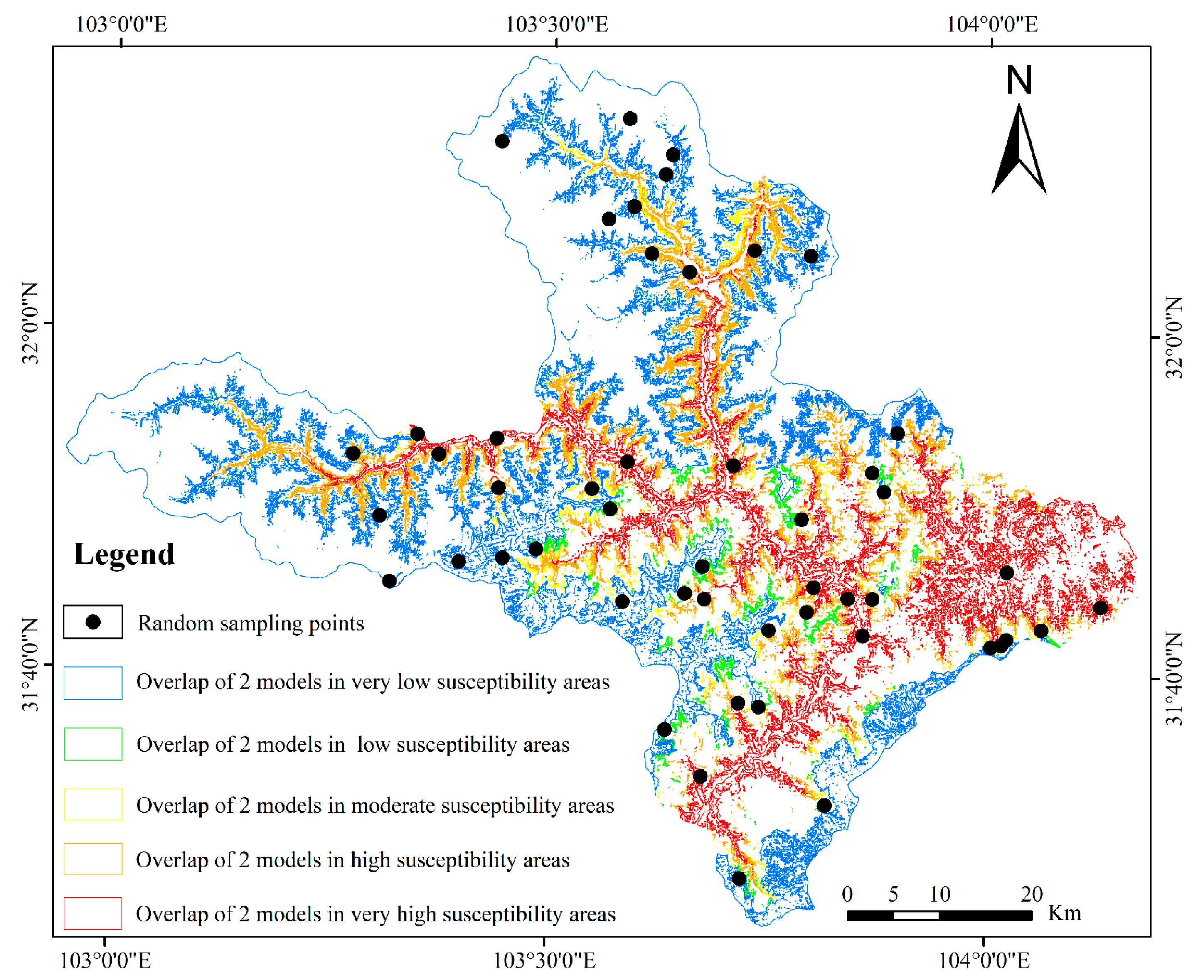
5.1. Comparison of Susceptibility Zoning Models in Mao
5.2. Analysis of Landslide Susceptibility Prediction Results in Mao
6. Conclusions
- The DNN model (accuracy = 88.6%, precision = 91.3%, recall = 94.8%, specificity = 87.8%, and F1-score = 93.0%) has the best performance in all criteria.
- The landslide susceptibility of Mao County after transfer learning successfully proves that the DNN model can improve the zoning of very-high-landslide-susceptibility areas, provide theoretical support for subsequent landslide investigations, and reduce the workload involved in fieldwork.
- The transfer learning method proposed in this paper shortens the work process of landslide susceptibility evaluation and is an unsupervised prediction tool for areas without landslide interpretation data, providing new ideas for landslide susceptibility evaluation. In the future, this research idea can be applied to other areas such as flooding and fire.
Author Contributions
Funding
Data Availability Statement
Conflicts of Interest
References
- Chen, W.; Li, Y. GIS-based evaluation of landslide susceptibility using hybrid computational intelligence models. Catena 2020, 195, 104777. [Google Scholar] [CrossRef]
- Huang, F.; Zhang, J.; Zhou, C.; Wang, Y.; Huang, J.; Zhu, L. A deep learning algorithm using a fully connected sparse autoen coder neural network for landslide susceptibility prediction. Landslides 2020, 17, 217–229. [Google Scholar] [CrossRef]
- Yang, W.; Qi, W.; Zhou, J. Decreased post-seismic landslides linked to vegetation recovery after the 2008 Wenchuan earthquake. Ecol. Indic. 2018, 89, 438–444. [Google Scholar] [CrossRef]
- Maheshwari, B. Spatial predictive modelling of rainfall-and earthquake-induced landslide susceptibility in the Himalaya region of Uttarakhand, India. Environ. Earth Sci. 2022, 81, 237. [Google Scholar]
- Huang, F.; Cao, Z.; Jiang, S.H.; Zhou, C.; Huang, J.; Guo, Z. Landslide susceptibility prediction based on a semi-supervised multiple-layer perceptron model. Landslides 2020, 17, 2919–2930. [Google Scholar] [CrossRef]
- Huang, F.; Yao, C.; Liu, W.; Li, Y.; Liu, X. Landslide susceptibility assessment in the Nantian area of China: A comparison of frequency ratio model and support vector machine. Geomat. Nat. Hazards Risk 2018, 9, 919–938. [Google Scholar] [CrossRef]
- Kavzoglu, T.; Sahin, E.K.; Colkesen, I. Landslide susceptibility mapping using GIS-based multi-criteria decision analysis, support vector machines, and logistic regression. Landslides 2014, 11, 425–439. [Google Scholar] [CrossRef]
- Huang, F.; Chen, L.; Yin, K.; Huang, J.; Gui, L. Object-oriented change detection and damage assessment using high-resolution remote sensing images, Tangjiao Landslide, Three Gorges Reservoir, China. Environ. Earth Sci. 2018, 77, 183. [Google Scholar] [CrossRef]
- Li, Y.; Huang, J.; Jiang, S.; Huang, F.; Chang, Z. A web-based GPS system for displacement monitoring and failure mechanism analysis of reservoir landslide. Sci. Rep. 2017, 7, 17171. [Google Scholar] [CrossRef]
- Huang, F.M.; Wu, P.; Ziggah, Y.Y. GPS Monitoring Landslide Deformation Signal Processing using Time-series Model. Int. J. Signal Process. Image Process. Pattern Recognit. 2016, 9, 321–332. [Google Scholar] [CrossRef]
- Wang, C.; Lin, Q.; Wang, L.; Jiang, T.; Su, B.; Wang, Y.; Mondal, S.K.; Huang, J.; Wang, Y. The influences of the spatial extent selection for non-landslide samples on statistical-based landslide susceptibility modelling: A case study of Anhui Province in China. Nat. Hazards 2022, 112, 1967–1988. [Google Scholar] [CrossRef]
- Wang, H.; Wang, L.; Zhang, L. Transfer learning improves landslide susceptibility assessment. Gondwana Res. 2023, 123, 238–254. [Google Scholar] [CrossRef]
- Ai, X.; Sun, B.; Chen, X. Construction of small sample seismic landslide susceptibility evaluation model based on Transfer Learning: A case study of Jiuzhaigou earthquake. Bull. Eng. Geol. Environ. 2022, 81, 116. [Google Scholar] [CrossRef]
- Fu, Z.; Li, C.; Yao, W. Landslide susceptibility assessment through TrAdaBoost transfer learning models using two landslide inventories. Catena 2023, 222, 106799. [Google Scholar]
- Li, Y.; Yang, J.; Han, Z.; Li, J.Y.; Wang, W.D.; Chen, N.S.; Hu, S.H.; Huang, J.L. An ensemble deep-learning framework for landslide susceptibility assessment using multiple blocks: A case study of Wenchuan area, China. Geomat. Nat. Hazards Risk 2023, 14, 2221771. [Google Scholar] [CrossRef]
- Yang, W.; Wang, D.; Chen, G. Reconstruction strategies after the Wenchuan Earthquake in Sichuan, China. Tour. Manag. 2011, 32, 949–956. [Google Scholar] [CrossRef]
- Gao, X.; Chen, T.; Fan, J. Analysis of the population capacity in the reconstruction areas of 2008 Wenchuan Earthquake. J. Geogr. Sci. 2011, 21, 521–538. [Google Scholar] [CrossRef]
- Qi, S.; Xu, Q.; Lan, H.; Zhang, B.; Liu, J. Spatial distribution analysis of landslides triggered by 2008.5.12 Wenchuan Earthquake, China. Eng. Geol. 2010, 116, 95–108. [Google Scholar] [CrossRef]
- Yan, L.; Gong, Q.; Wang, F.; Chen, L.; Li, D.; Yin, K. Integrated Methodology for Potential Landslide Identification in Highly Vegetation-Covered Areas. Remote Sens. 2023, 15, 1518. [Google Scholar] [CrossRef]
- Du, J.; Glade, T.; Woldai, T.; Chai, B.; Zeng, B. Landslide susceptibility assessment based on an incomplete landslide inventory in the Jilong Valley, Tibet, Chinese Himalayas. Eng. Geol. 2020, 270, 105572. [Google Scholar] [CrossRef]
- Wang, Z.; Xu, S.; Liu, J.; Wang, Y.; Ma, X.; Jiang, T.; He, X.; Han, Z. A Combination of Deep Autoencoder and Multi-Scale Residual Network for Landslide Susceptibility Evaluation. Remote Sens. 2023, 15, 653. [Google Scholar] [CrossRef]
- Meena, S.R.; Puliero, S.; Bhuyan, K.; Floris, M.; Catani, F. Assessing the importance of conditioning factor selection in landslide susceptibility for the province of Belluno (region of Veneto, northeastern Italy). Nat. Hazard. Earth Sys. 2022, 22, 1395–1417. [Google Scholar] [CrossRef]
- Piloyan, A.; Konečný, M. Semi-Automated Classification of Landform Elements in Armenia Based on SRTM DEM using K-Means Unsupervised Classification. Quaest. Geogr. 2017, 36, 93–103. [Google Scholar] [CrossRef]
- Deng, H.; Wu, X.; Zhang, W.; Liu, Y.; Li, W.; Li, X.; Zhou, P.; Zhuo, W. Slope-Unit Scale Landslide Susceptibility Mapping Based on the Random Forest Model in Deep Valley Areas. Remote Sens. 2022, 14, 4245. [Google Scholar] [CrossRef]
- Bragagnolo, L.; Silva, R.V.D.; Grzybowski, J.M.V. Artificial neural network ensembles applied to the mapping of landslide susceptibility. Catena 2020, 184, 104240. [Google Scholar] [CrossRef]
- Fang, H.; Shao, Y.; Xie, C.; Tian, B.; Shen, C.; Zhu, Y.; Guo, Y.; Yang, Y.; Chen, G.; Zhang, M. A New Approach to Spatial Landslide Susceptibility Prediction in Karst Mining Areas Based on Explainable Artificial Intelligence. Sustainability 2023, 15, 3094. [Google Scholar] [CrossRef]
- Huang, F.; Cao, Z.; Guo, J.; Jiang, S.; Li, S.; Guo, Z. Comparisons of heuristic, general statistical and machine learning models for landslide susceptibility prediction and mapping. Catena 2020, 191, 104580. [Google Scholar] [CrossRef]
- Hua, Y.; Wang, X.; Li, Y.; Xu, P.; Xia, W. Dynamic development of landslide susceptibility based on slope unit and deep neural networks. Landslides 2021, 18, 281–302. [Google Scholar] [CrossRef]
- Esposito, C.; Mastrantoni, G.; Marmoni, G.M.; Antonielli, B.; Caprari, P.; Pica, A.; Schilirò, L.; Mazzanti, P.; Bozzano, F. From theory to practice: Optimisation of available information for landslide hazard assessment in Rome relying on official, fragmented data sources. Landslides 2023, 20, 2055–2073. [Google Scholar] [CrossRef]
- Chen, X.; Chen, W. GIS-based landslide susceptibility assessment using optimized hybrid machine learning methods. Catena 2021, 196, 104833. [Google Scholar] [CrossRef]
- Chang, Z.; Du, Z.; Zhang, F.; Huang, F.; Chen, J.; Li, W.; Guo, Z. Landslide Susceptibility Prediction Based on Remote Sensing Images and GIS: Comparisons of Supervised and Unsupervised Machine Learning Models. Remote Sens. 2020, 12, 502. [Google Scholar] [CrossRef]
- Shirzadi, A.; Bui, D.T.; Pham, B.T.; Solaimani, K.; Chapi, K.; Kavian, A.; Shahabi, H.; Revhaug, I. Shallow landslide susceptibility assessment using a novel hybrid intelligence approach. Environ. Earth Sci. 2017, 76, 60. [Google Scholar] [CrossRef]
- Erener, A.; Düzgün, H.S.B. Landslide susceptibility assessment: What are the effects of mapping unit and mapping method? Environ. Earth Sci. 2012, 66, 859–877. [Google Scholar] [CrossRef]
- Zhao, H.; Yao, L.; Mei, G.; Liu, T.; Ning, Y. A Fuzzy Comprehensive Evaluation Method Based on AHP and Entropy for a Landslide Susceptibility Map. Entropy 2017, 19, 396. [Google Scholar] [CrossRef]
- Yong, C.; Jinlong, D.; Fei, G.; Bin, T.; Tao, Z.; Hao, F.; Li, W.; Qinghua, Z. Review of landslide susceptibility assessment based on knowledge mapping. Stoch. Environ. Res. Risk Assess. 2022, 36, 399–417. [Google Scholar] [CrossRef]
- Marjanović, M.; Kovačević, M.; Bajat, B.; Voženílek, V. Landslide susceptibility assessment using SVM machine learning algorithm. Eng. Geol. 2011, 123, 225–234. [Google Scholar] [CrossRef]
- Kong, C.; Tian, Y.; Ma, X.; Weng, Z.; Zhang, Z.; Xu, K. Landslide Susceptibility Assessment Based on Different MaChine Learning Methods in Zhaoping County of Eastern Guangxi. Remote Sens. 2021, 13, 3573. [Google Scholar] [CrossRef]
- Azarafza, M.; Azarafza, M.; Akgün, H.; Atkinson, P.M.; Derakhshani, R. Deep learning-based landslide susceptibility mapping. Sci. Rep. 2021, 16, 24112. [Google Scholar] [CrossRef]
- Rong, G.; Li, K.; Su, Y.; Tong, Z.; Liu, X.; Zhang, J.; Zhang, Y.; Li, T. Comparison of Tree-Structured Parzen Estimator Optimization in Three Typical Neural Network Models for Landslide Susceptibility Assessment. Remote Sens. 2021, 13, 4694. [Google Scholar] [CrossRef]
- Jiang, S.; Huang, J.; Huang, F.; Yang, J.; Yao, C.; Zhou, C. Modelling of spatial variability of soil undrained shear strength by conditional random fields for slope reliability analysis. Appl. Math. Model. 2018, 63, 374–389. [Google Scholar] [CrossRef]
- Chang, Z.; Catani, F.; Huang, F.; Liu, G.; Meena, S.R.; Huang, J.; Zhou, C. Landslide susceptibility prediction using slope unit-based machine learning models considering the heterogeneity of conditioning factors. J. Rock Mech. Geotech. Eng. 2023, 15, 1127–1143. [Google Scholar] [CrossRef]
- Yu, X.; Wang, Y.; Niu, R.; Hu, Y. A Combination of Geographically Weighted Regression, Particle Swarm Optimization and Support Vector Machine for Landslide Susceptibility Mapping: A Case Study at Wanzhou in the Three Gorges Area, China. Int. J. Environ. Res. Public Health 2016, 13, 487. [Google Scholar] [CrossRef] [PubMed]
- Ullah, K.; Wang, Y.; Fang, Z.; Wang, L.; Rahman, M. Multi-hazard susceptibility mapping based on Convolutional Neural Networks. Geosci. Front. 2022, 13, 101425. [Google Scholar] [CrossRef]
- Fang, Z.; Wang, Y.; Duan, H.; Niu, R.; Peng, L. Comparison of general kernel, multiple kernel, infinite ensemble and semi-supervised support vector machines for landslide susceptibility prediction. Stoch. Environ. Res. Risk Assess. 2022, 36, 3535–3556. [Google Scholar] [CrossRef]
- Yuan, R.; Chen, J. A novel method based on deep learning model for national-scale landslide hazard assessment. Landslides 2023, 20, 2379–2403. [Google Scholar] [CrossRef]
- Lu, J.; Behbood, V.; Hao, P.; Zuo, H.; Xue, S.; Zhang, G. Transfer learning using computational intelligence: A survey. Knowl. Syst. 2015, 80, 14–23. [Google Scholar] [CrossRef]
- Huang, F.; Tao, S.; Li, D.; Lian, Z.; Catani, F.; Huang, J.; Li, K.; Zhang, C. Landslide Susceptibility Prediction Considering Neighborhood Characteristics of Landslide Spatial Datasets and Hydrological Slope Units Using Remote Sensing and GIS Technologies. Remote Sens. 2022, 14, 4436. [Google Scholar] [CrossRef]
- Huang, F.; Xiong, H.; Yao, C.; Catani, F.; Zhou, C.; Huang, J. Uncertainties of landslide susceptibility prediction considering different landslide types. J. Rock Mech. Geotech. Eng. 2023, 15, 2954–2972. [Google Scholar] [CrossRef]
- Cody, T.; Beling, P.A. A Systems Theory of Transfer Learning. IEEE Syst. J. 2023, 17, 26–37. [Google Scholar] [CrossRef]
- Fanaja, R.A.; Saputri, M.E.; Pradana, M. Knowledge as a mediator for innovativeness and risk-taking tolerance of female entrepreneurs in Indonesia. Cogent Soc. Sci. 2023, 9, 2185989. [Google Scholar] [CrossRef]
- Tekin, S.; Çan, T. Slide type landslide susceptibility assessment of the Büyük Menderes watershed using artificial neural network method. Environ. Sci. Pollut. Res. 2022, 29, 47174–47188. [Google Scholar] [CrossRef] [PubMed]
- Bi, X.; Fan, Q.; He, L.; Zhang, C.; Diao, Y.; Han, Y. Analysis and Evaluation of Extreme Rainfall Trends and Geological Hazards Risk in the Lower Jinshajiang River. Appl. Sci. 2023, 13, 4021. [Google Scholar] [CrossRef]


| Data Name | Type | Spatial Resolution | Uses of Data | Source |
|---|---|---|---|---|
| UAV Images | Raster | 2 | Landslide interpretation | \ |
| Landslide points | Vector | \ | Test result verification | Sichuan General Geological and Environmental Monitoring Station |
| Geographic data | Vector | 1:250,000 | Extraction of roads and rivers | National Geomatics Center of China |
| Digital elevation model | Raster | 30 | Extraction of slopes, aspects, etc. | Geospatial Data Cloud |
| Geological data | Raster | 1:250,000 | Extraction of structural line | Bureau of Geological Survey of Sichuan Province |
| Influencing Factor | ||
|---|---|---|
| Elevation | 0.337 | 2.966 |
| Slope | 0.109 | 9.211 |
| Aspect | 0.994 | 1.006 |
| Curvature | 0.996 | 1.004 |
| Topographic relief | 0.109 | 9.181 |
| Distance to roads | 0.141 | 7.068 |
| Distance to rivers | 0.156 | 6.418 |
| Distance to tectonic lines | 0.916 | 1.092 |
| Hardware/Software | Parameters |
|---|---|
| CPU | Intel Xeon E5-2680 v3 (Intel, Santa Clara, CA, USA) |
| GPU | NVIDIA GeForce RTX 2080Ti (NVIDIA Corporation, Santa Clara, CA, USA) |
| Operating Memory | 256 GB |
| Total Video Memory | 60 GB |
| Operating System | Ubuntu 18.04 |
| Python | Python 3.6 |
| IDE | PyCharm 2020.1 (Professional Edition) |
| CUDA | CUDA 10.0 |
| CUDNN | CUDNN 7.6.5 |
| Deep Learning Architecture | PyTorch 1.2.0 |
| Factor | Weight |
|---|---|
| Elevation | 2.241 |
| Slope | −5.076 |
| Aspect | −0.993 |
| Curvature | −6.219 |
| Topographic relief | 7.321 |
| Distance to tectonic lines | −5.112 |
| Distance to rivers | 0.091 |
| Distance to roads | 0.547 |
| Parameters | Values |
|---|---|
| Epochs | 500 |
| Dropout | 0.5 |
| Learning rate | 0.001 |
| Number of hidden layers | 5 |
| Dense connection | 512/1024/1024/2048/2048/2 |
| Activation function | ReLU |
| Optimizer | Adam |
| Loss function | Binary cross-entropy |
| Indicators | SVM | DNN |
|---|---|---|
| TP | 10,521 | 11,352 |
| TN | 8852 | 10,516 |
| FP | 3127 | 1463 |
| FN | 1458 | 627 |
| Accuracy (%) | 77.1 | 88.6 |
| Precision (%) | 80.9 | 91.3 |
| Recall (%) | 87.8 | 94.8 |
| Specificity (%) | 73.9 | 87.8 |
| F1-score (%) | 84.2 | 93.0 |
| Aim | Code Block |
|---|---|
| Importing factors of Mao | data = pd.read_excel(“maoxian.xlsx”) |
| Reading all data in the set | data_model = data.values |
| Importing the pre-trained model | model = load_model(“model_best.h5”) |
| Model prediction | data model predict = model.predict(data model) |
| Model | Zoning Level | Percentage of Landslides (%) | Percentage of Graded Area (%) | Ri |
|---|---|---|---|---|
| SVM | I | 4.4 | 49.5 | 0.09 |
| II | 13.6 | 17.1 | 0.79 | |
| III | 17.7 | 11.8 | 1.5 | |
| IV | 26 | 10.6 | 2.45 | |
| V | 38.3 | 11 | 3.48 | |
| DNN | I | 1.5 | 47.7 | 0.03 |
| II | 0.1 | 3.1 | 0.03 | |
| III | 0.3 | 6.4 | 0.05 | |
| IV | 13.3 | 18.7 | 0.71 | |
| V | 84.8 | 24.1 | 3.52 |
| Model | Longitude | Latitude | Prediction | Susceptibility Zoning |
|---|---|---|---|---|
| SVM | 103°34′53.4″ | 32°12′20.952″ | 0.002964 | Very low |
| DNN | 0.229454 | |||
| SVM | 103°26′6″ | 32°10′55.6314″ | 0.030296 | |
| DNN | 0.196198 | |||
| SVM | 103°53′32.9994″ | 31°54′3.456″ | 0.118348 | Low |
| DNN | 0.301761 | |||
| SVM | 103°51′50.04″ | 31°51′42.948″ | 0.133782 | |
| DNN | 0.327504 | |||
| SVM | 103°35′16.08″ | 32°7′11.7474″ | 0.310471 | Moderate |
| DNN | 0.47144 | |||
| SVM | 103°39′8.2794″ | 32°3′23.6154″ | 0.325105 | |
| DNN | 0.493688 | |||
| SVM | 104°0′48.24″ | 31°41′39.264″ | 0.524868 | High |
| DNN | 0.622887 | |||
| SVM | 103°44′50.2794″ | 31.70707 | 0.527368 | |
| DNN | 0.620217 | |||
| SVM | 103°42′17.9994″ | 31°52′3.9″ | 0.77524 | Very High |
| DNN | 0.91976 | |||
| SVM | 103°51′18″ | 31°42′9.324″ | 0.7722 | |
| DNN | 0.880981 |
Disclaimer/Publisher’s Note: The statements, opinions and data contained in all publications are solely those of the individual author(s) and contributor(s) and not of MDPI and/or the editor(s). MDPI and/or the editor(s) disclaim responsibility for any injury to people or property resulting from any ideas, methods, instructions or products referred to in the content. |
© 2024 by the authors. Licensee MDPI, Basel, Switzerland. This article is an open access article distributed under the terms and conditions of the Creative Commons Attribution (CC BY) license (https://creativecommons.org/licenses/by/4.0/).
Share and Cite
Wang, X.; Wang, D.; Li, X.; Zhang, M.; Cheng, S.; Li, S.; Dong, J.; Xu, L.; Sun, T.; Li, W.; et al. The Prediction of Cross-Regional Landslide Susceptibility Based on Pixel Transfer Learning. Remote Sens. 2024, 16, 347. https://doi.org/10.3390/rs16020347
Wang X, Wang D, Li X, Zhang M, Cheng S, Li S, Dong J, Xu L, Sun T, Li W, et al. The Prediction of Cross-Regional Landslide Susceptibility Based on Pixel Transfer Learning. Remote Sensing. 2024; 16(2):347. https://doi.org/10.3390/rs16020347
Chicago/Turabian StyleWang, Xiao, Di Wang, Xinyue Li, Mengmeng Zhang, Sizhi Cheng, Shaoda Li, Jianhui Dong, Luting Xu, Tiegang Sun, Weile Li, and et al. 2024. "The Prediction of Cross-Regional Landslide Susceptibility Based on Pixel Transfer Learning" Remote Sensing 16, no. 2: 347. https://doi.org/10.3390/rs16020347