
Self-Supervised Transformers for Unsupervised SAR Complex Interference Detection Using Canny Edge Detector
by
 ,
,
Yugang Feng
1,2,3,
Bing Han
1,2,3,4,*,
Xiaochen Wang
1,2,4,
Jiayuan Shen
1,2,3,
Xin Guan
1,2,4 and
Hao Ding
1,2,4 1
Aerospace Information Research Institute, Chinese Academy of Sciences, Beijing 100094, China
2
Key Laboratory of Technology in Geo-Spatial Information Processing and Application System, Chinese Academy of Sciences, Beijing 100190, China
3
School of Electronic, Electrical and Communication Engineering, University of Chinese Academy of Sciences, Beijing 101408, China
4
Key Laboratory of Target Cognition and Application Technology, Chinese Academy of Sciences, Beijing 100094, China
*
Author to whom correspondence should be addressed.
Remote Sens. 2024, 16(2), 306; https://doi.org/10.3390/rs16020306
Submission received: 11 December 2023
/
Revised: 4 January 2024
/
Accepted: 9 January 2024
/
Published: 11 January 2024
(This article belongs to the Special Issue Advances in Synthetic Aperture Radar Image Processing and Information Extraction)
Abstract
:As the electromagnetic environment becomes increasingly complex, a synthetic aperture radar (SAR) system with wideband active transmission and reception is vulnerable to interference from devices at the same frequency. SAR interference detection using the transform domain has become a research hotspot in recent years. However, existing transform domain interference detection methods exhibit unsatisfactory performance in complex interference environments. Moreover, most of them rely on label information, while existing publicly available interference datasets are limited. To solve these problems, this paper proposes an SAR unsupervised interference detection model that combines Canny edge detection with vision transformer (CEVIT). Using a time–frequency spectrogram as input, CEVIT realizes interference detection in complex interference environments with multi-interference and multiple types of interference by means of a feature extraction module and a detection head module. To validate the performance of the proposed model, experiments are conducted on airborne SAR interference simulation data and Sentinel-1 real interference data. The experimental results show that, compared with the other object detection models, CEVIT has the best interference detection performance in a complex interference environment, and the key evaluation indexes (e.g., Recall and F1-score) are improved by nearly 20%. The detection results on the real interfered echo data have a Recall that reaches 0.8722 and an F1-score that reaches 0.9115, which are much better than those of the compared methods, and the results also indicate that the proposed model achieves good detection performance with a fast detection speed in complex interference environments, which has certain practical application value in the interference detection problem of the SAR system.

1. Introduction
A synthetic aperture radar (SAR) is a piece of wideband microwave remote sensing equipment that acquires high-resolution images through the active transmission and reception of electromagnetic signals. However, with the wide application of microwave remote sensing technology, when operating, SAR is vulnerable to interference from devices in the same frequency band, the electromagnetic environment is becoming more and more complex, and spectrum resources are becoming more and more scarce. Generally, the energy of this interference is much larger than the energy of the target signals, which leads to a significant degradation in the quality of the SAR imaging [1,2,3,4,5]. At the same time, with the rapid development of interference technology, a variety of interference techniques are constantly proposed, resulting in difficulty maintaining stable performance of SAR systems in the complex interference environment. The complex interference environment refers to the simultaneous existence of multiple or more types of interference, and the power of these interference signals may vary with a certain range. However, there are relatively few existing studies on statistical characterization and detection for SAR complex interference [1,6,7]. In the conventional signal or echo domain, some scholars have utilized the statistical characteristics of the signal for interference detection. Wang et al. [8] used approximate spectral decomposition to divide the spectrum into multiple sampling bands and compared each sub-band with the threshold; if the power of the sub-band is higher than the threshold, the sub-band is considered to contain interference, and the sub-band samples are deleted to achieve interference mitigation. Natsuaki et al. [9] proposed an interference detection method for a pulse signal SAR system with a relatively large time–bandwidth product. They employed local autocorrelation-based detection in the range–time and azimuth–frequency domains. Leng et al. [2] conducted experiments on C-band SAR Sentinel-1 data, utilized the scattering characteristics whereby co-polarization is generally larger than cross-polarization in the common backscatter coefficient of the Earth, and proposed a radio frequency interference (RFI) index based on the dual-polarization difference design of RFIs, which is capable of detecting RFIs and locating them better by using the ground range detected (GRD) data, by taking advantage of the unique RFI characteristics of dual-polarization GRD images. At present, interference detection based on traditional methods is usually used to detect interference much stronger than the real signal, and the detection results cannot be well obtained when the interference-to-signal ratio is relatively low. At the same time, most of them have a certain limitation on the detection environment [1,7,8]; thus, the detection effect is not satisfactory in the complex interference environment. In recent years, with the development of computer-related technologies, artificial intelligence technology represented by deep learning has been widely used in various fields, and intelligent analysis and interpretation based on data in the field of remote sensing have become trends for future development [10]. The powerful learning ability of deep learning and the ability to deal with massive data classification make it highly promising for applications in interference detection. Using deep learning to learn and think about the statistical properties of interference to achieve interference detection in complex interference environments has become a hotspot in current research.
After receiving the SAR echoes, the data are sampled and stored. Data processing is a two-dimensional process, but it is typically separated into two independent one-dimensional processing steps: the range processing and the azimuth processing. Some researchers have transformed signal processing from the signal domain to the transform domain (e.g., frequency domain, time–frequency domain, or image domain), moving from one-dimensional processing in the signal domain to two-dimensional processing in the image domain in recent years, and designed a deep learning network to realize the interference detection by using multi-layer convolutional neural networks (CNN) [11,12,13,14,15,16]. The interference detection problem in the transform domain can be categorized as a target detection problem. Noting that the single-shot multibox detector algorithm has not yet been applied to the interference detection and suppression problem, Yu et al. [11] utilized short-time Fourier transform (STFT) to transform the SAR echoes into the time–frequency domain and trained the model using pre-labeled datasets to achieve the detection of multiple types of interference, parameter estimation, and interference suppression. Tao et al. [16] proposed a semantic cognitive enhancement network for interference detection. The network combines dilated spatial pyramid pooling, deep convolution, and self-attention mechanisms. The method does not require a pre-set threshold and does not require a large number of training samples. Experiments are conducted on different scenes of Sentinel-1 images containing multiple types of interference to verify the robustness of the model’s detection performance. So far, most of the deep-learning-based interference detection networks are supervised learning approaches, which require training sets, test sets, and validation sets, while there are fewer publicly available interference-containing SAR datasets, resulting in the need for manual annotation during the construction of the datasets. Moreover, supervised learning can only capture information about interference that is already labeled in the dataset, and the power and type of interference in the actual data have a certain randomness, which may lead to supervised learning models only being suitable for use in a specific dataset or unlabeled interference types appearing to be missed.
Unsupervised learning is one of the most challenging and significant problems in computer vision and machine learning today, where unsupervised learning models reveal the intrinsic properties and patterns of data and enable prediction by learning from unlabeled samples. In recent years, transformer networks have developed rapidly; compared with CNNs, the attention mechanism in transformer networks can deal with long-distance dependencies better, and the model is more portable. These advantages make more and more research begin to focus on how to apply transformer networks in computer vision [17,18,19,20,21,22,23,24,25,26,27,28]. Research has also made some progress in unsupervised learning of transformer networks in target detection. Caron et al. [25] proposed an end-to-end target detection method where the model uses self-distillation loss for self-supervised learning. The model is interpreted as a form of self-distillation with no labels (DINO). It established a teacher network and a student network, achieving a high-accuracy attention map and fully unsupervised semantic segmentation on transformer networks. This resulted in state-of-the-art performance on public object detection datasets at the time. Siméoni et al. [26] used the DINO self-supervised pre-training model to obtain the feature maps. They calculated similarity scores between each patch and its adjacent patches, selecting the patch with the fewest similar patches as the initial seed for positioning the starting point of target localization. They used the similarity scores to connect and build a binary target segmentation mask, ultimately achieving object detection. The model locates objects in images without any labels, resulting in a significant performance improvement compared to state-of-the-art methods. Wang et al. [27] proposed a graph-based algorithm that used the features obtained by a self-supervised transformer to detect and segment salient objects in images (Tokencut). With this approach, the image patches that compose an image are organized into a fully connected graph, where the edge between each pair of patches is labeled with a similarity score between patches using features learned by the transformer, and then normalized cuts are used to group self-similar regions and delineate foreground objects. Wang et al. [28] proposed a zero-shot unsupervised multi-object detection method. The method utilizes features extracted by the DINO model, repeatedly employs the Tokencut to generate masks for multiple objects, and uses these masks as ground truth. For the problem wherein ground truth masks obtained by self-supervised model will miss some ground truth, a dynamic loss descent strategy is used to detect the objects missed by the ground truth masks, and the performance is further improved by multiple self-training. Many scientific experiments have demonstrated the advantages of a pre-trained vision transformer (VIT) as a backbone network for feature extraction in object detection, while less research has been performed in the field of SAR interference detection using unsupervised learning of a VIT, and the possibility of utilizing pre-trained VITs for feature extraction and detection of complex interference in the transform domain has become a point of interest for us.
The paper proposes an unsupervised interference detection model for a vision transformer combined with Canny edge detection (CEVIT) and conducts experiments on datasets containing complex interference and a lower interference-to-signal ratio (ISR). The experimental results show that CEVIT achieves the best performance with both a lower ISR and complex interference compared to other detection methods.
The main contributions of this paper are:
- Aiming at the problem wherein existing interference detection problems still require a large amount of manually annotated information, an unsupervised interference detection model is proposed to achieve interference detection end to end without any labeled information;
- For the lower ISR, a feature fusion module based on multi-head attention is proposed, which achieves better results in the lower-ISR environment while integrating multi-head attention features;
- For the case of complex interference with multiple numbers and types, a detection head module combining Canny edge detection and a transformer network is proposed, further extending the applicability of the interference detection model;
- An SAR time–frequency spectrogram dataset for a complex interference environment is established.
The rest of the paper is organized as follows: Section 2 models the echo signal and performs time–frequency characterization. Section 3 describes the proposed model in detail. Section 4 presents the data used in the experiments and experimental results with the comparison. Section 5 discusses the experimental results and considers future works. Section 6 summarizes the work of this paper.
2. Signal Time–Frequency Characterization
2.1. Echo Signal Model
For a normal working SAR system, the received echo signals include real signals, noise signals, and interference signals. The noise signal mainly comes from the environment, and the interference signal mainly comes from other strong radiation sources in the same frequency band. Generally, the energy of interference is much greater than that of both the target signal and noise; both noise signals and interference signals can be expressed as additive influences, and, thus, the interfered echo signal S is modeled as Equation (1) [11,15]:
where is the time unit in the range, is the th pulse in the azimuth, is the target signals, is the noise signals, and is the interference signals.
The SAR high-resolution imaging process is subject to diverse and complex interference, which seriously affects the final imaging results of the SAR. Interference is classified according to the energy source, bandwidth, and modulation type, etc. According to the energy source of the interference, it can be divided into two categories: passive interference and active interference. Typical passive interference includes chaff interference, wave-absorbing materials, anti-radar camouflage nets, and so on. Active interference refers to the interference generated by the energy source radiating electromagnetic waves, mainly including enemy active interference signals, wireless communication signals, radio and television signals, and other radar signals. According to the relative bandwidth of the interference relative to the SAR bandwidth, it can be divided into wideband interference and narrowband interference. Wideband interference generally has a bandwidth greater than 10% of the transmitted signal [4,7]. In this paper, interference bandwidth signals that are less than 10% of the transmitted signal are considered as narrowband interference. Categorized according to the type of modulation, there are various types of actual modulation, the most common being chirp modulation and sin modulation, among others.
In order to better approximate a real complex interference environment, this paper models and uses the following interference signals: single-frequency interference (noted as ), narrowband chirp-modulated interference (noted as ), wideband chirp-modulated interference (noted as ), narrowband sinusoidal-modulated interference (noted as ), and wideband sinusoidal-modulated interference (noted as ). The expression for the interference signals is as follows:
where is the time unit in the range, is the th pulse in the azimuth, , , , and stand for single frequency interference, narrowband chirp -modulated interference, wideband chirp-modulated interference, narrowband sinusoidal-modulated interference, and wideband sinusoidal-modulated interference, respectively. The difference between wideband and narrowband is the cumulative number of interfered echoes; in this paper, single-frequency interference, chirp-modulated interference, and sinusoidal-modulated interference are modeled.
The single-frequency interference can be expressed as:
where is the number of single frequency interference, , and represent the amplitude, frequency and initial phase of the interference, respectively.
The chirp modulated interference can be expressed as:
where represents the number of chirp modulated interference, , and stand for the amplitude, the frequency, and the chirp rate of the th interference, respectively.
The sinusoidal modulated interference can be expressed as:
where stands for the number of sinusoidal modulated interference, , , and represent the amplitude, modulation coefficient, the frequency, and the initial phase of the th interference, respectively.
After a thorough analysis and modeling of the echo signals and interference signals, we proceed to analyze how to use transform domain features and extract interference characteristics.
2.2. Echo Time–Frequency Characterization
The time–frequency characteristics of the echo signal are analyzed using the transform domain, and the commonly used transform domains are the frequency domain, time–frequency domain, etc. Frequency domain analysis is the use of Fourier transform to transform the signal to the frequency domain; frequency domain analysis can be obtained for the overall frequency components of the signal. Commonly used methods for time–frequency domain analysis are short-time Fourier transform (STFT), etc. For unknown appearing interference, in order to obtain its time–frequency characteristics in a smoother way, the universality feature of STFT is exploited, by dividing the signal into shorter time segments and using Fourier transform (FT) for these segments, which enables us to observe the spectral characteristics of the signal in different time segments. The expression for STFT [11] is:
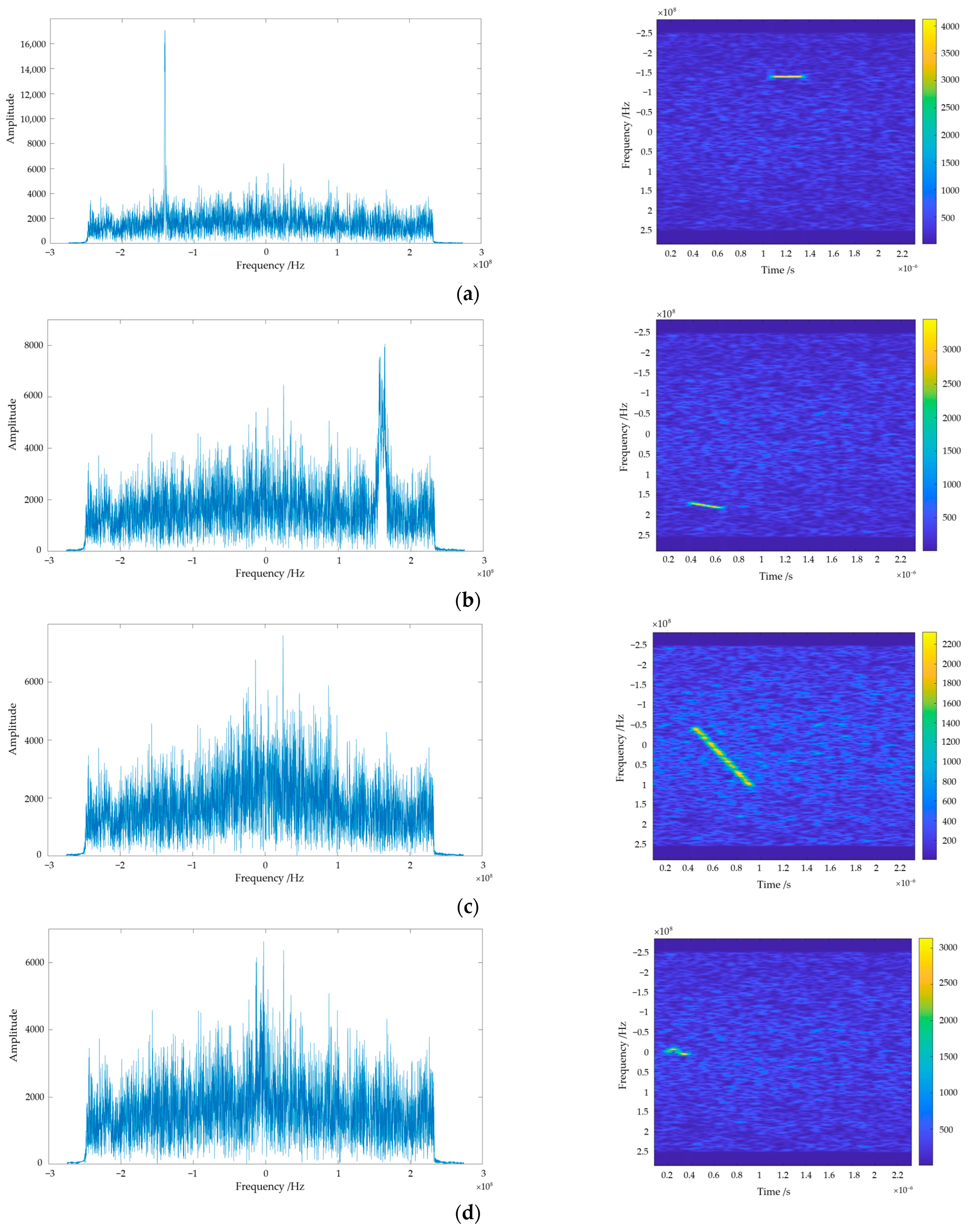
where represents the time-frequency spectrogram of signals, and stand for the number of sampling points in the time domain and frequency domain, represents the th time domain signal, denotes the conjugate form of the window function, represents total number of sample. The interference signal established in this paper is characterized using frequency domain analysis and time–frequency analysis, and the results of both analyses are shown in Figure 1.
According to Figure 1a–e, it is obvious that the frequency domain analysis is able to show the single-frequency and narrowband chirp modulation interference more distinctly, whereas the characterization information is not well captured when facing other types of interference. This is because frequency domain analysis is good at dealing with signals with more stable frequency characteristics. But, for non-stationary signals, frequency domain analysis can only tell us what frequency components are in the signal. Time–frequency analysis can reflect the frequency components of the signal more intuitively, we can distinguish between different types of interference through the time–frequency spectrogram, and we can obtain the time–frequency characteristics of the interference very well.
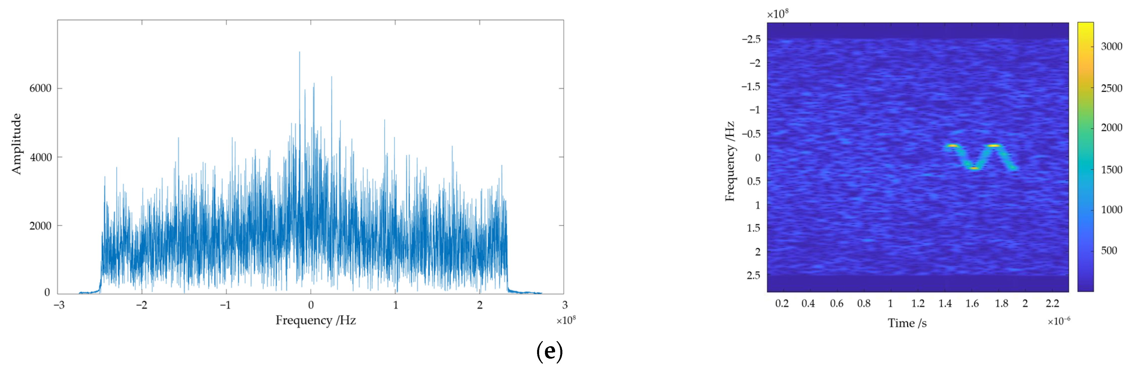
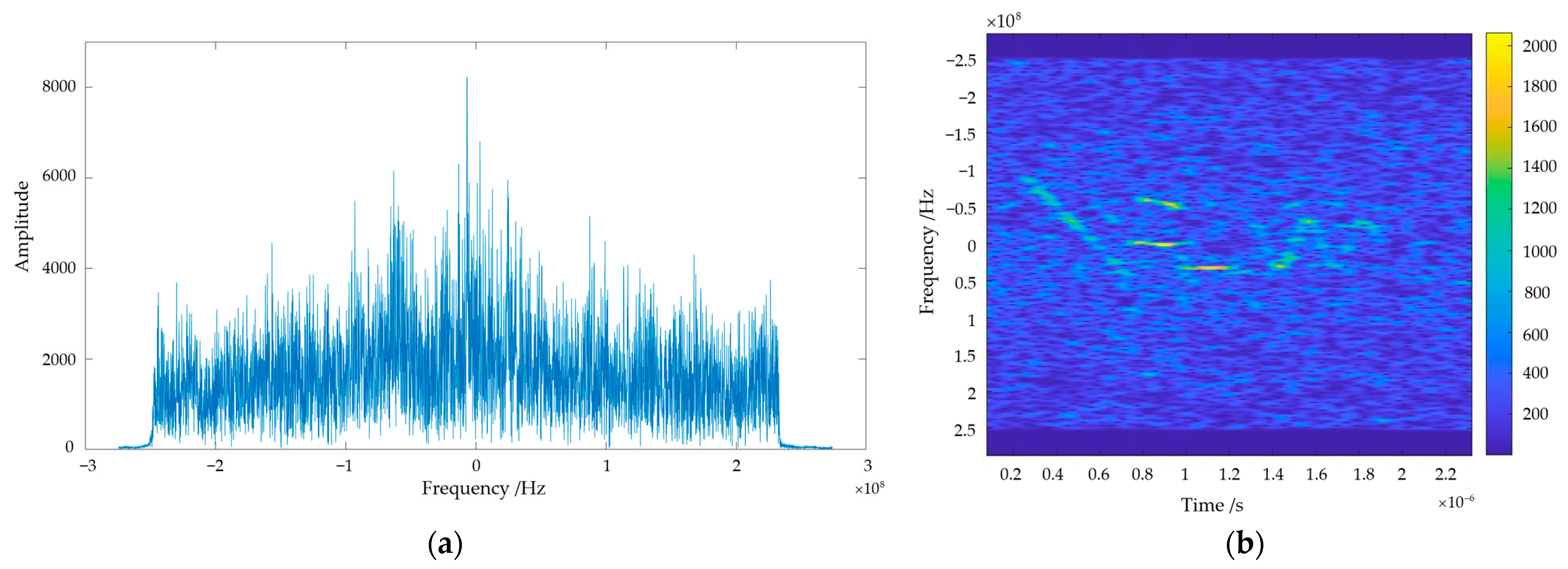
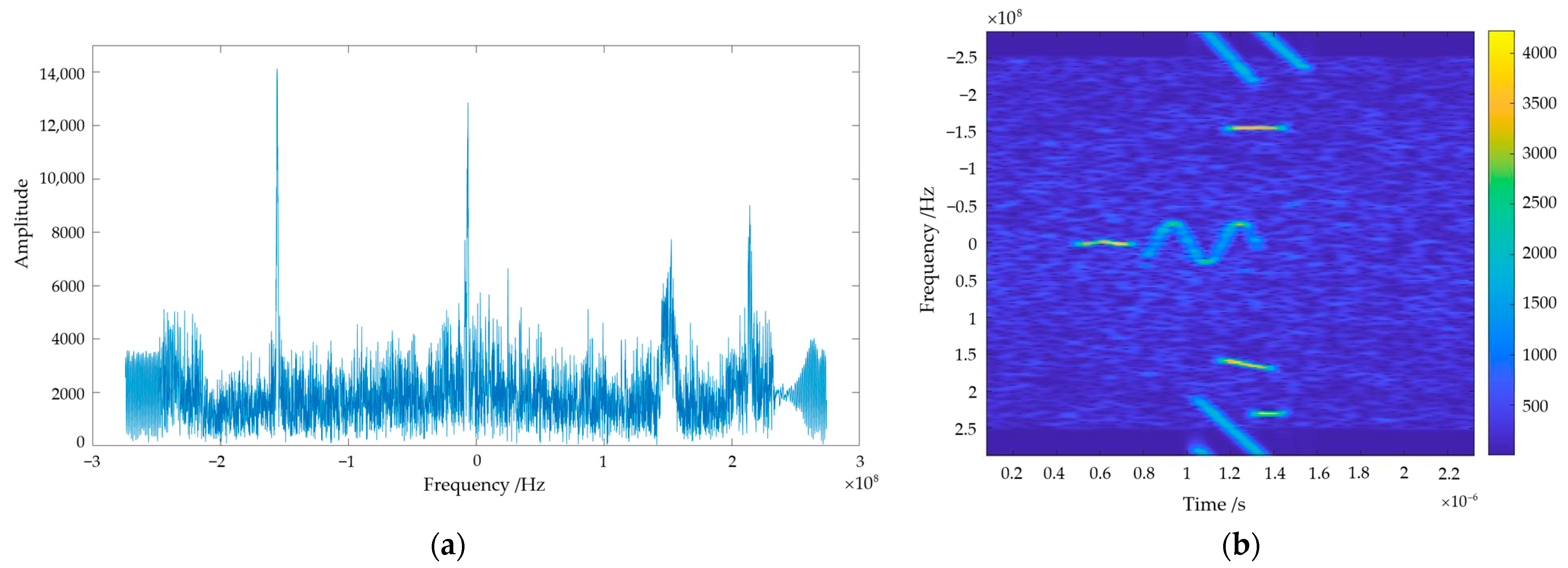
For the complex interference echo signal established in this paper, frequency domain analysis and time–frequency analysis are used to characterize the interference signal. The analysis results of the two methods at a lower and higher ISR, respectively, are shown in Figure 2 and Figure 3.
Through comparison, it can be clearly seen that, when faced with complex interference, frequency domain analysis can only obtain information about which frequency components the signal encompasses as a whole, lacking details about the appearance time of individual components. Moreover, if the signal parameters have agility and exhibit complexity, frequency domain analysis struggles to capture information effectively. Conversely, interference in the time–frequency spectrograms exhibits prominent edge features, indicating distinct pixel transitions in the interfered regions. Simultaneously, distinctive characteristics of each frequency component are clearly visible in these spectrograms.
Based on the above analysis, the time–frequency spectrogram has the following advantages over the frequency spectrum:
- It can reflect the interference characteristic information more intuitively. Using STFT to analyze the non-smooth signal, we can well obtain the time, instantaneous frequency, and amplitude of the appearance of each component of the signal, and also the change of signal frequency with time;
- The time–frequency spectrogram contains strong edge feature information. There are relatively pronounced pixel transitions, which provide information for interference detection and localization.
3. Methods and Model
Based on the modeling and analysis results in the second section, we observed that interference detection based on time–frequency representations exhibits strong visual characteristics. Furthermore, the excellent performance of visual transformer networks in recent years in computer vision tasks encouraged us to use a transformer network as the backbone for feature extraction. During experiments, we noticed that the multi-head attention mechanism in visual transformers assigns different levels of attention to various types of interference. To avoid unnecessary loss, we designed and utilized a feature fusion module to combine the multi-head attention feature maps. We also noticed that time–frequency representations possess strong edge features, even in scenarios with a low ISR and complex interference types. These representations exhibit noticeable pixel transitions. Consequently, we designed and used a detection head module that combines edge detection and bounding box generation strategies. The module extracts interference edge features, facilitating interference localization and labeling and ultimately producing the final detection results.
This section first gives the overall framework of the SAR unsupervised interference detection model that combines Canny edge detection with a vision transformer (CEVIT) and then goes into detail on each of the key components.
3.1. Overall Framework
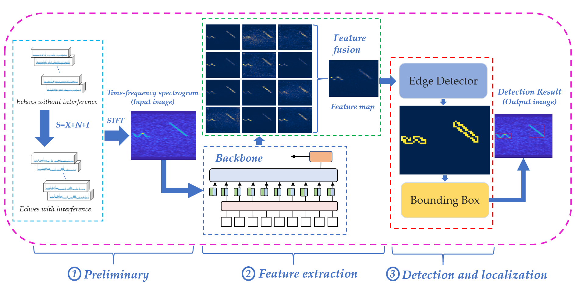
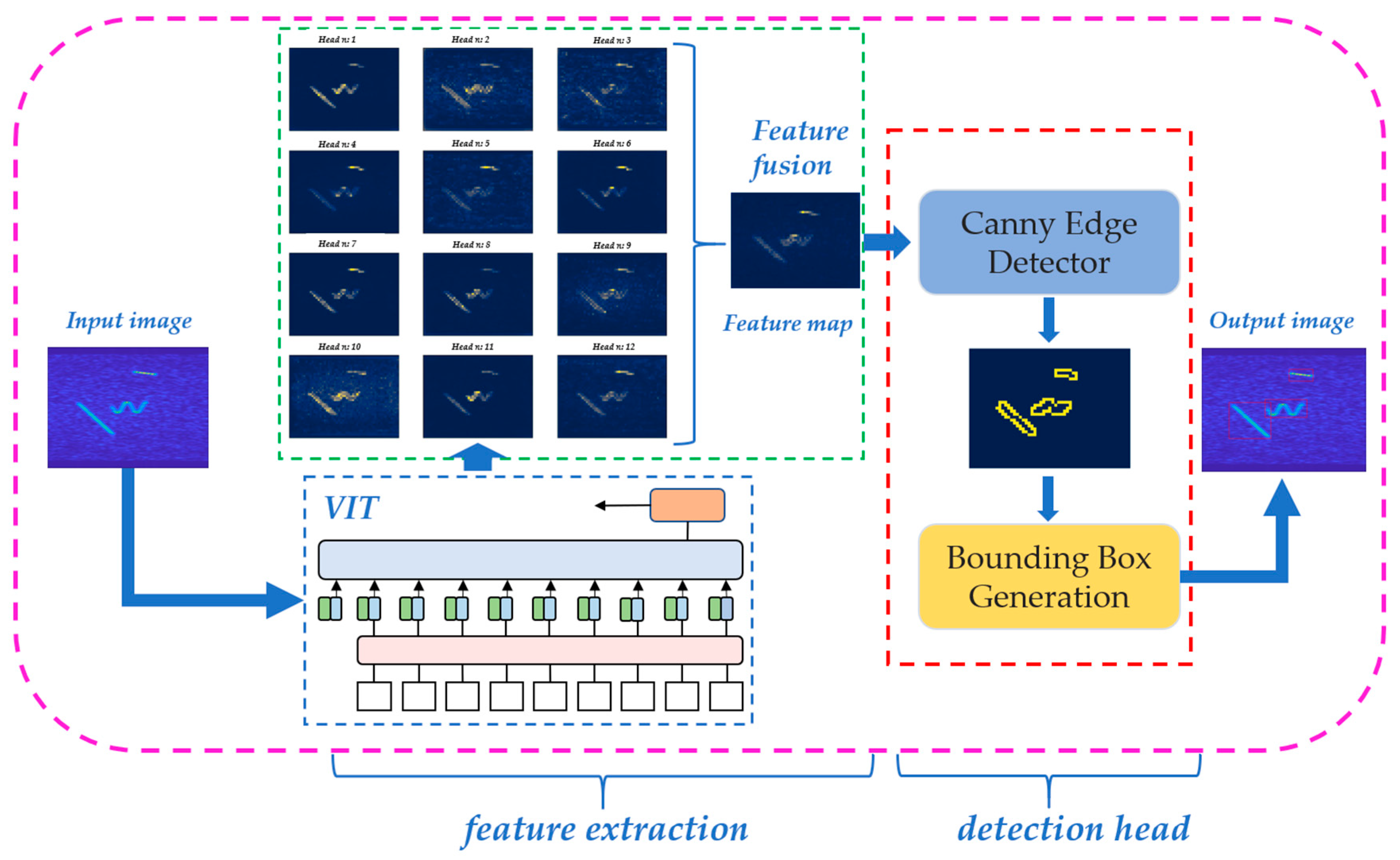
Similar to the object detection framework, the interference detection network is composed of backbone and detection head [29,30,31]. Interference detection work consists of two main components: a feature extraction module and a detection head module, as shown in Figure 4.
The feature extraction module is to extract features from the model input using a deep learning network and obtain the feature map. The interference detection head module is to locate and find the bounding box of interference in the feature map and finally output the result after marking the interference.
3.2. Feature Extraction Module
The feature extraction module consists of two main parts: the backbone and the feature fusion block.
3.2.1. Backbone
The backbone used to extract the features is the transformer structure. Dosovitskiy et al. [18] proposed a vision transformer (VIT) to apply the transformer structure in image classification in the field of computer vision. The core idea is to use the transformer framework to process the images using non-overlapping patches as tokens. The whole transformer network can be divided into two parts; one part is the feature extraction part, and the other part is the classification part. In the feature extraction part, the input size of image is divided into patches of size, and then the whole image is divided into non-overlapping patches, and then the divided patch is used as a token and embedded with location information. At the same time, an additional learnable token (noted as class token) is added into the sequence of images, and the patch token and the class token are fed into the transformer encoder as embedded tokens for feature extraction. The transformer encoder is composed of a number of transformer blocks, which are feedforward networks consisting of a self-attention structure and layer normalization [32]. In the process of extraction, the class token will interact with other features for feature interaction, fusing features from other image sequences. In the classification phase, the class token, after extracting features from the self-attention, is fully connected to achieve classification. For the CEVIT, we used the semi-supervised learning transformer network proposed in DINO [24] for feature extraction.
3.2.2. Feature Fusion Block
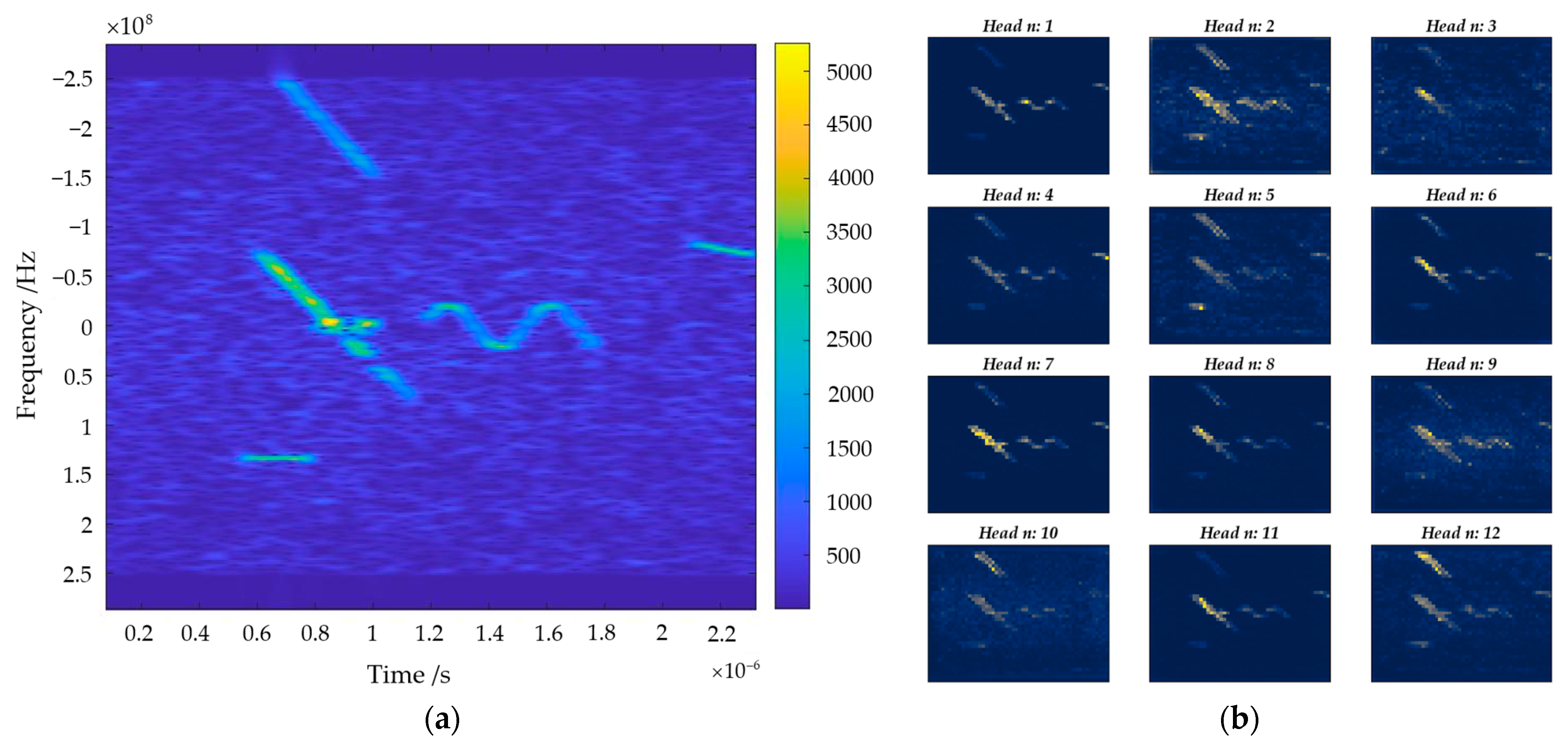
The feature fusion block is designed to synthesize the advantages of the acquired features to obtain more detailed information. The previous work used only one feature from the last attention layer of the model as the output feature of the model in the feature extraction part (for example, one of the Key, Query, and Value features) [26,27,28]. Multiple attention [33] allows models to co-attend to information from different representational subspaces at different locations. We note that multi-head attention mechanism of the transformer network also outputs attention features, and each attention head focuses on different aspects of the same image, as shown in Figure 5 below.
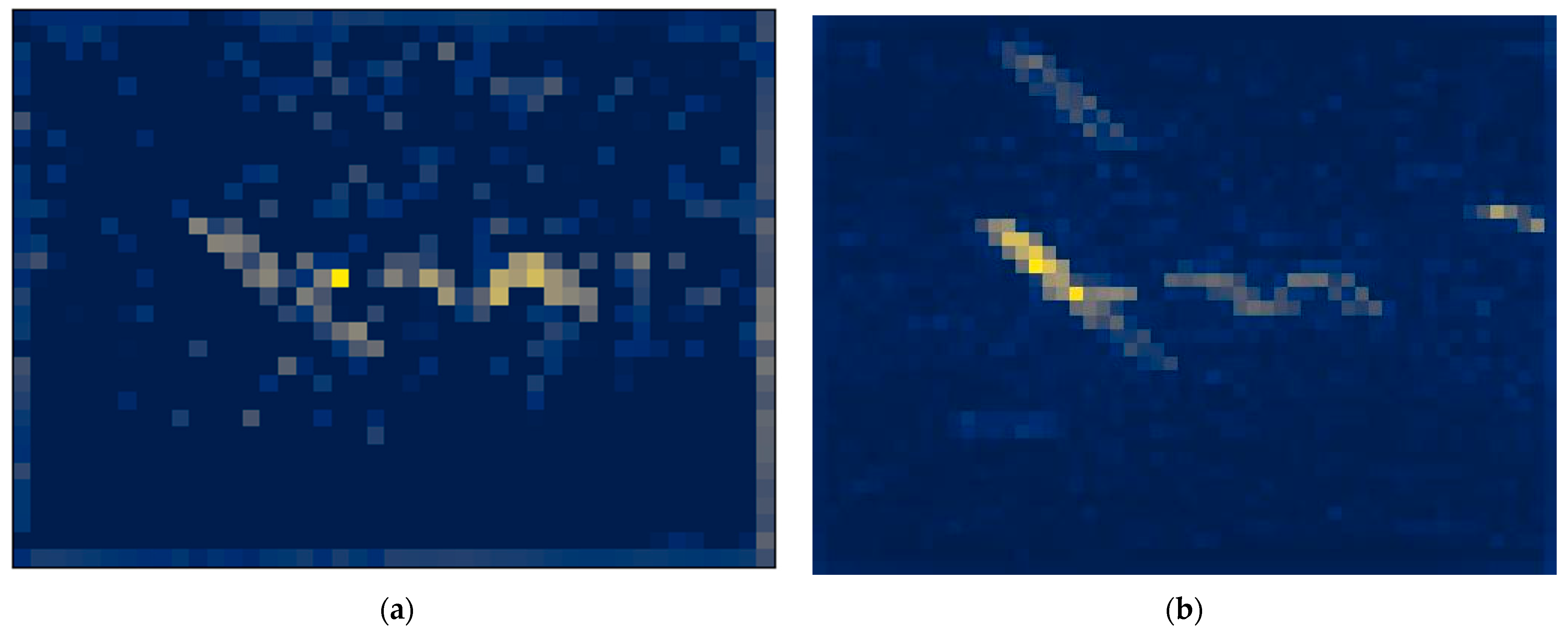
To avoid the loss of information that might result from the use of a single feature, the paper proposes a multi-head attention feature fusion block that averages all the multi-head attention features and takes the fused feature map as the output of the whole feature extraction module. The results of the comparison between the single feature map (K feature, for example) and the fused feature map are shown in Figure 6 (take Figure 5a as an example of an input image).
The feature map indicates how much attention the model pays to the image, with blue indicating less attention and yellow indicating more attention. It can be clearly seen that, compared to a single feature (K feature, for example), the fused feature map contains less noise and pays more attention to the interference in the time–frequency spectrogram, which is conducive to subsequent interference localization and framing. Thus, in this paper, we used the fused feature map as the input to the subsequent detection head module.
3.3. Detection Head Module
The detection head module consists of two main parts: Canny edge detection and detection box generation strategy. Canny edge detection is to highlight the regions in the image where the pixel changes are obvious and then locate the regions of interference in the image. The detection frame generation strategy is to generate the interference detection frame and output the detection result according to the specified rules.
3.3.1. Canny Edge Detection
The Canny edge detection algorithm was first proposed by Canny et al. [34]. Among the current common edge detection methods, Canny edge detection is one with a well-defined, reliable approach, which can be divided into the following four steps:
- Apply Gaussian filter to remove image noise: In order to minimize the impact of noise on edge detection results, noise needs to be filtered out to prevent false detections caused by noise using a Gaussian filter convolved with the image to smooth the image;
- Calculate the gradient strength and direction: Determine the edges based on the gradient value and gradient direction of the image, i.e., calculate the location with the strongest change in grayscale;
- Eliminate false detections by using non-maximum suppression: The non-maximum suppression [35] is to make blurred edges clear by comparing the gradient strength of the pixel with the pixels in the positive and negative directions of the gradient direction of the pixel and retaining the pixel if it has the largest gradient strength or setting it to 0. After traversing the whole image, a thin line with the brightest color will be retained in the edges;
- Dual-threshold boundary detection: Using the upper and lower boundaries of the threshold, the pixels in the image are determined as edges and non-edges, and all the edge pixels are retained as real edges to form the final edge detection result.
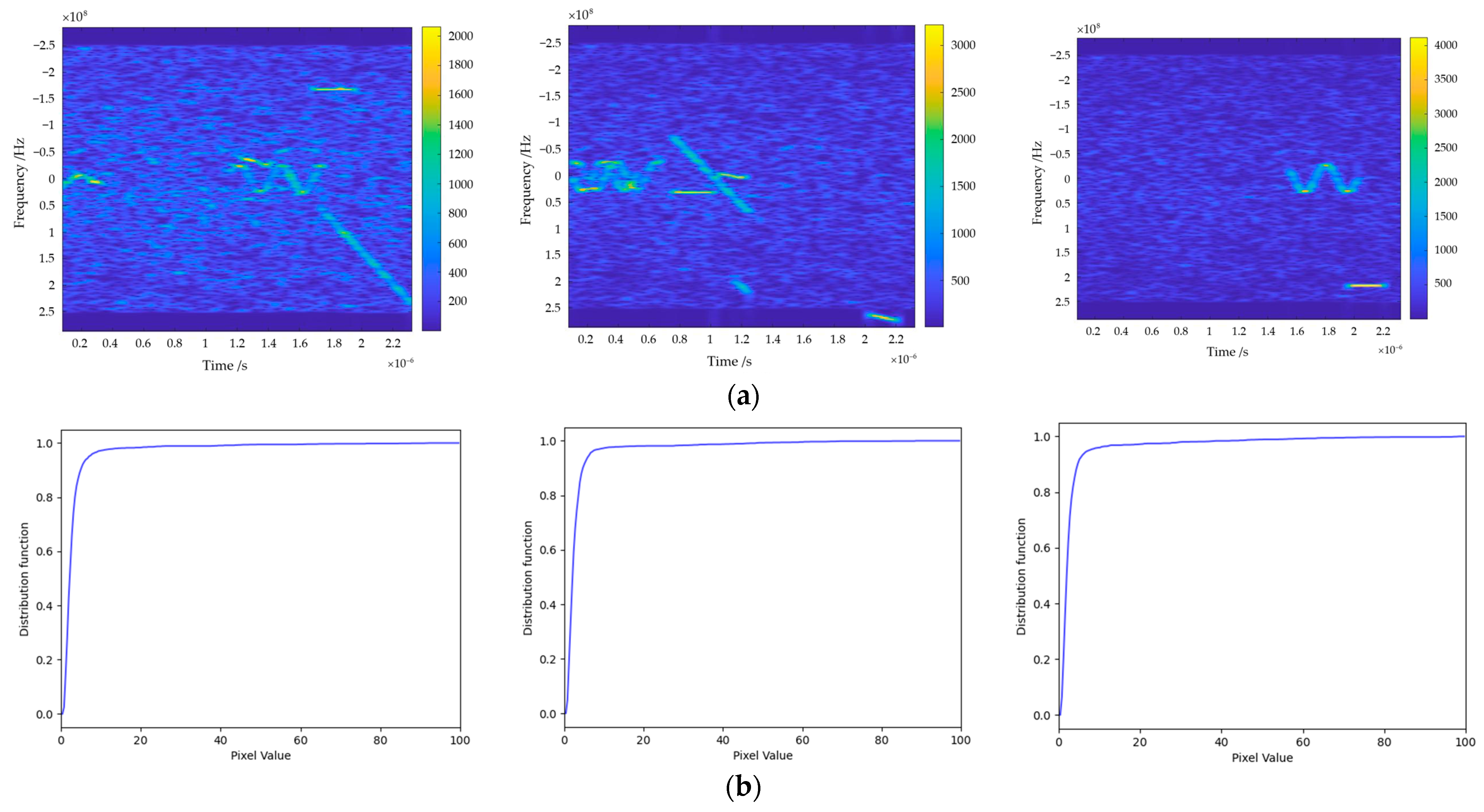
In the edge detection stage, we noted two factors that affect the efficiency of subsequent interference detection and localization: the size of the convolution kernel of the Gaussian filter and the dual-threshold boundary. The size of the convolution kernel affects the computational speed. A large convolutional kernel can cover a larger area of the input image, which helps to capture global features and structural information, but it requires more parameters, which increases the complexity and computational cost of the model, and, at the same time, it is easy to lose the detailed information of the interference in the case of a lower ISR. Smaller convolutional kernels can better capture local features and texture of the input image, and can obtain more detailed information when facing the interference of parameter shortcuts, and, thus, in this paper, when choosing the commonly used Gaussian convolutional kernels, we chose smaller convolutional kernels to filter out image noise. The dual-threshold boundary affects the accuracy of edge detection, i.e., it affects the accuracy of the detection box. In the experimental process, we noticed that the percentage of the interfered region in the time–frequency spectrogram for the data used in the experiments is much smaller than that of the not-interfered region, and, at the same time, the pixel value in the time–frequency diagram tends to stabilize after the pixel value is close to 10, i.e., there is only a small portion of pixels higher than this value. At the same time, in order to avoid the misdetection caused by the appearance of the individual strong-point targets in the time–frequency spectrogram, the authors set the lower bound of the double-threshold detection at 15. Separately, the distribution function of pixels for different ISRs is shown in Figure 7 (from left to right, the ISRs are 5 dB, 8 dB, and 10 dB, respectively).
After Canny edge detection, the interfered edge pixels in the feature map will be highlighted, and the pixels that are connected to each other and the number of connections greater than 1 are detected by using the connectivity domain so as to form a number of closed, unconnected blocks of highlighted pixels in the feature map and to complete the localization of the interference in the edge detection.
3.3.2. Detection Box Generation Strategy
After generating the edge detection results, the detection box generation strategy traverses the locations of the highlighted pixel blocks in the whole feature map. We consider the highlighted pixel blocks on the feature map as the interference to be detected. At the same time, by setting the detection protection interval to 1, the ones that are larger than the detection protection interval are considered to be different interference; and, vice versa, they are considered to be the same interference. In this way, the location of different interference is recorded, and the interference detection box is generated to output the final time–frequency spectrogram interference detection result.
4. Experiments and Results
This section first constructs the dataset used for experiments and then introduces the evaluation metrics employed in this paper. Finally, the performance of the proposed model is validated through experiments on both simulated and real data.
4.1. Dataset Preparation
The data used in the experiments consist of X-band airborne SAR echo data and C-band European Space Agency (ESA) Sentinel-1 echo data. The basic parameters are shown in Table 1.
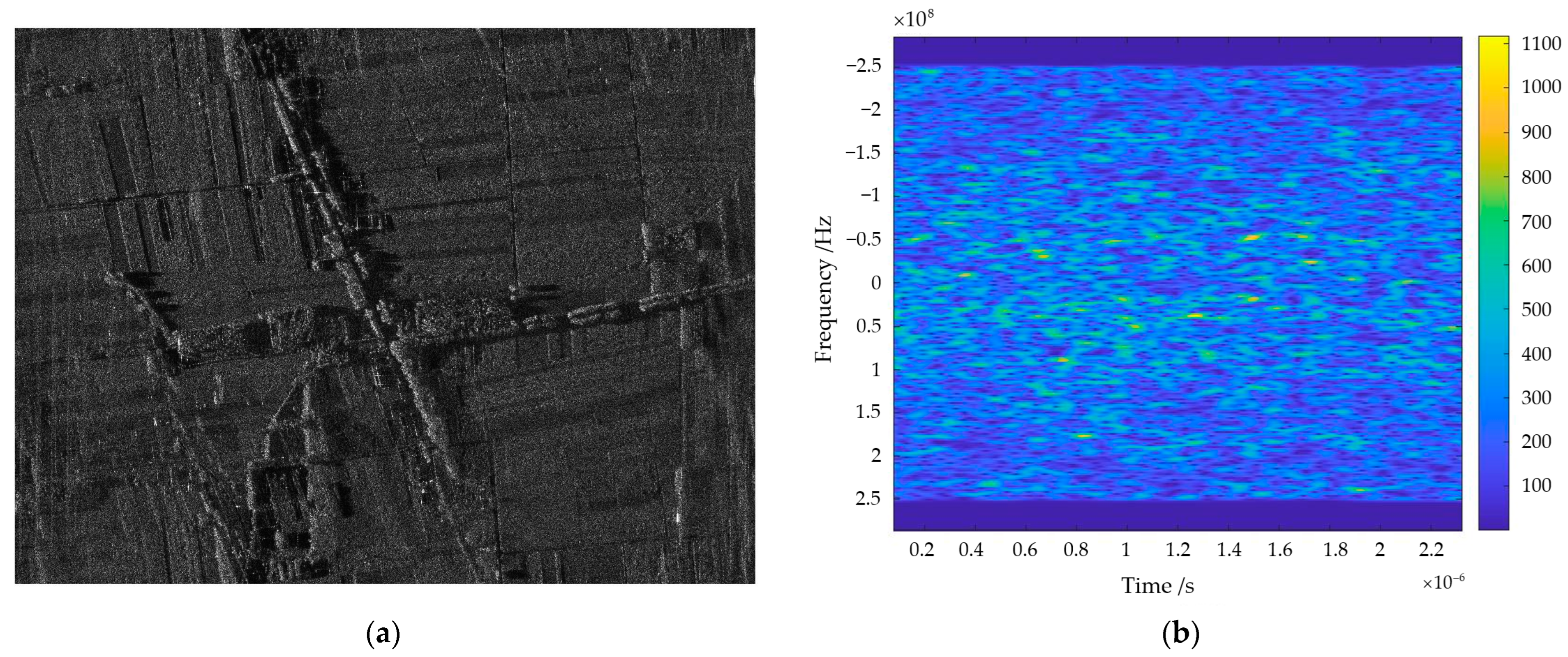
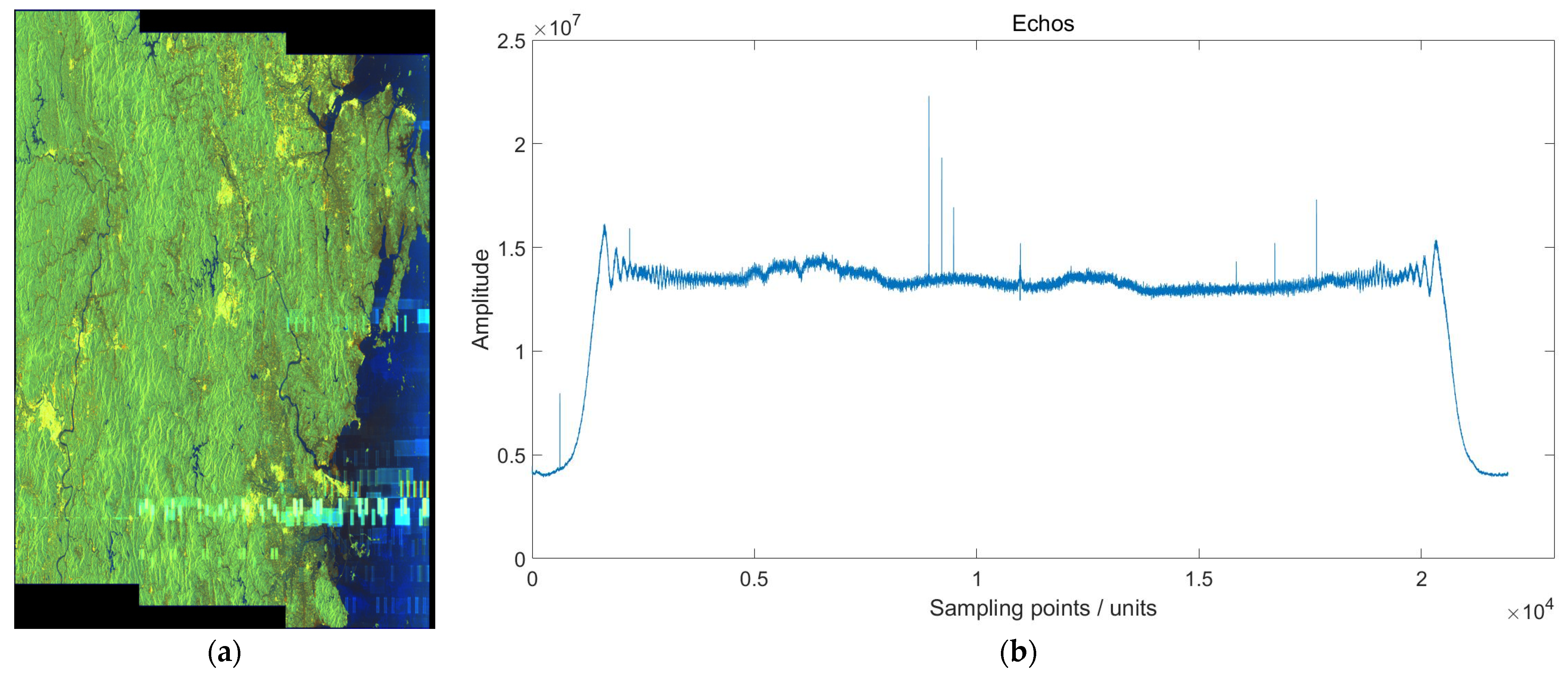
The imaging result and original time–frequency spectrogram of the raw echo data of the airborne SAR are shown in Figure 8.
Adding interference to the airborne SAR echo data, Equation (1) can be expressed as follows:
where is the time unit in the range, is the th pulse in the azimuth, repersents the uninterfered echo signal. The formula used in this paper to calculate the interference-to-signal ratio (ISR) is defined here:
where is the time unit in the range, is the th pulse in the azimuth represents interfered echoes, represents the uninterfered echo signal. According to Equation (8), the interference is added to the echoes after the de-carrier frequency, and the ISR is between 5 and 10 dB. The specific parameters and types are shown in the Table 2 below.
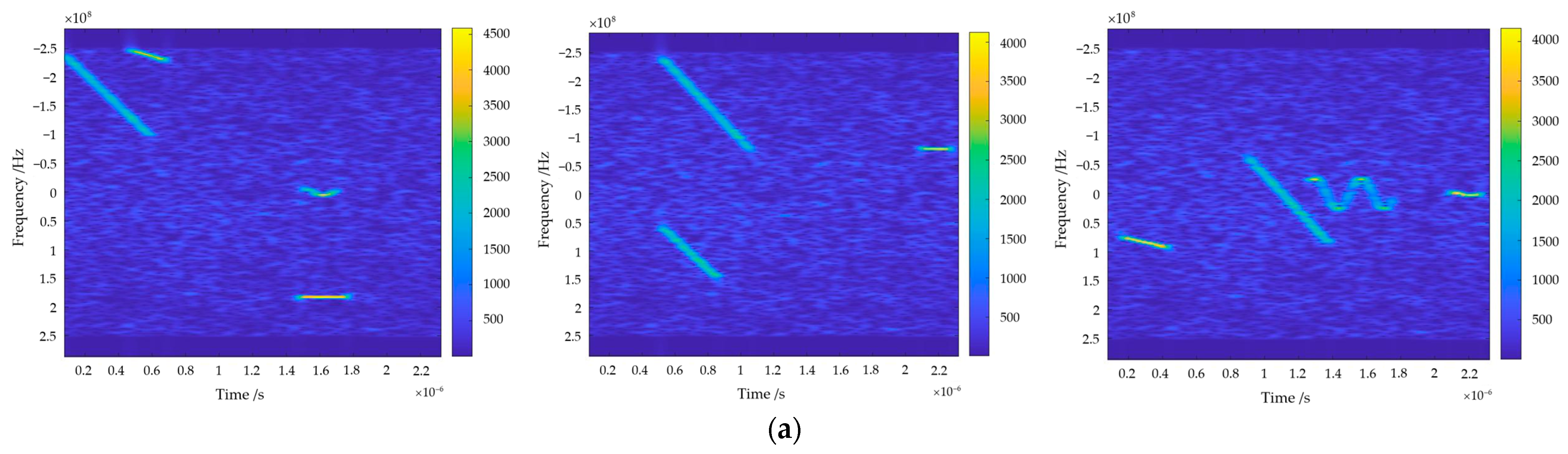
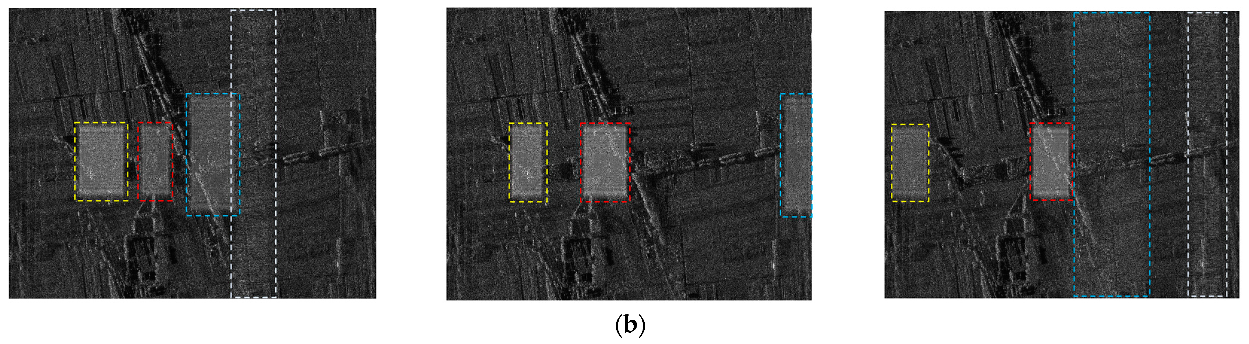
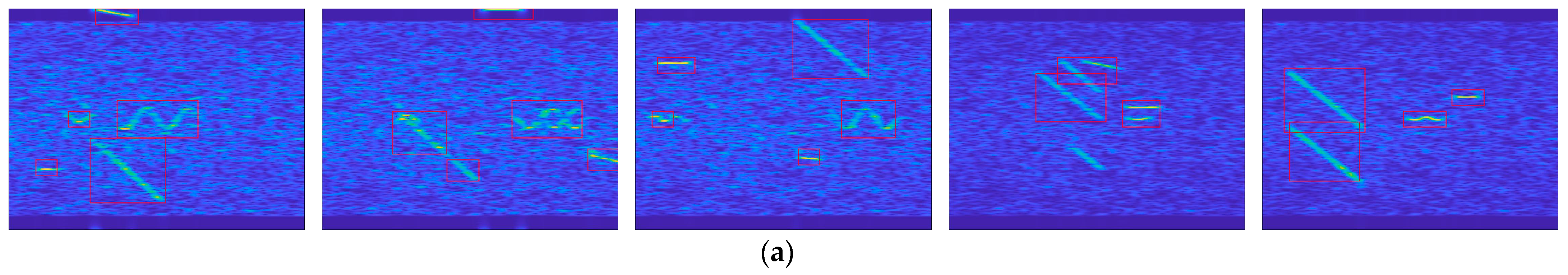
The simulation data of airborne SAR interfered echoes under different ISRs are established by using the above parameters. Some of the time–frequency spectrogram and imaging results of the interfered echoes are shown in Figure 9, and the dashed box in Figure 9b marks the location of the interference.
Real interfered echo data from the ESA’s Sentinel-1: The SAR data used in the experiment come from Sentinel-1, with Sentinel-1A launched on 3 April 2014 as the first environmental monitoring satellite in the Copernicus program. Sentinel-1B was successfully launched on 25 April 2016, allowing both satellites to operate simultaneously, effectively doubling observation efficiency with a repeat cycle of 6 days. On 23 December 2021, the ESA and the European Commission announced that it was the end of the mission for Sentinel-1B. The data used in this experiment are the original echo data from Sentinel-1B in Interferometric Wide Swath (IW) mode on 15 April 2020. The interfered image domain and the overall interfered echo are shown in Figure 10.
The experimental dataset is composed of a test set without annotations and a validation set with annotations. The test set contains airborne SAR echo data at different ISRs, including 1000 interference time–frequency spectrograms from each ISR, totaling 5000 images. The validation set is 30% randomly selected from the airborne SAR echo data with annotation information added, along with 133 real Sentinel-1 interfered data. The total number of images in the validation set is 1633 with annotation information.
4.2. Evaluation Index and Experimental Details
To validate the detection performance, evaluation indexes are established using , , and frame per second (FPS), in this paper, FPS denotes the time required each time-frequency spectrogram to be detected, and the expressions of , , are as follows:
where represents true positive; is false positive; stands for false negative. The terms , , and are calculated from the Intersection over Union () between the bounding boxes of ground truth and the bounding boxes of prediction as follows:
where represents the bounding boxes of detection result; stands for the bounding boxes of ground truth.
To validate the performance of the proposed model in this paper, we evaluate the model by comparing several unsupervised target detection models, including LOST, Cutler, and Tokencut, while evaluating the models based on visual results for the test dataset and numerical results using evaluation indexes on the validation dataset.
The experiments are conducted using the PyTorch 1.11.0 framework on a computer running Ubuntu 20.0 with a CUDA version 11.3 and an RTX 3080 GPU for testing and validation. The input and output image sizes are set to 875 × 656, and the experiments use a VIT model pre-trained on ImageNet with DINO [24] VIT-B version, patch size 16 × 16. The Canny edge detection uses a Gaussian convolution kernel size of 3 × 3 [36,37], and the dual-threshold range is set to [15, 80]. In the interference detection, any pixel block highlighted by the edge detection with more than 1 is considered candidate interference, and the protection interval for interference detection is set to 1. is considered true positive.
4.3. Experimental Results
4.3.1. Test Set Detection Results
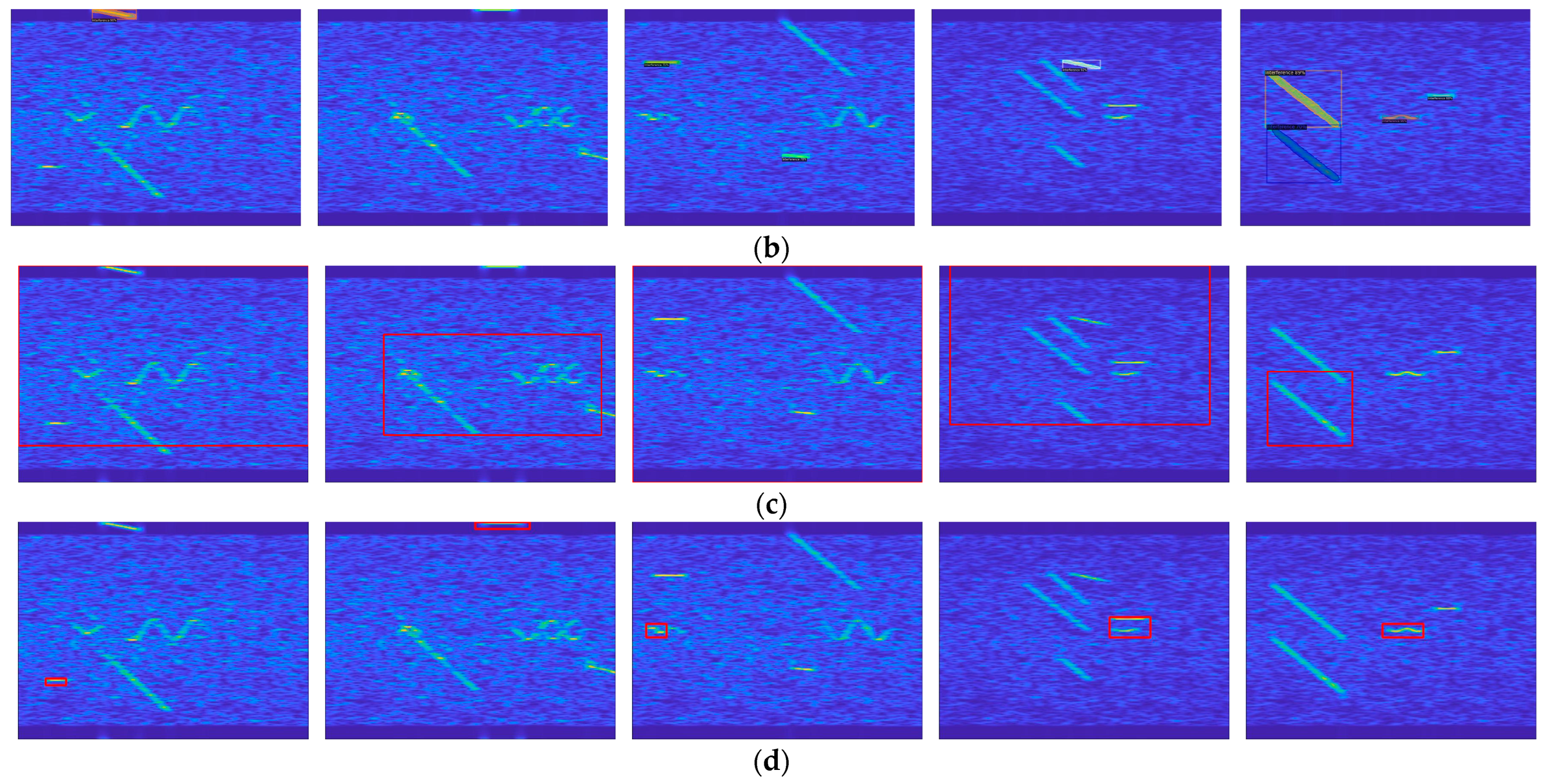
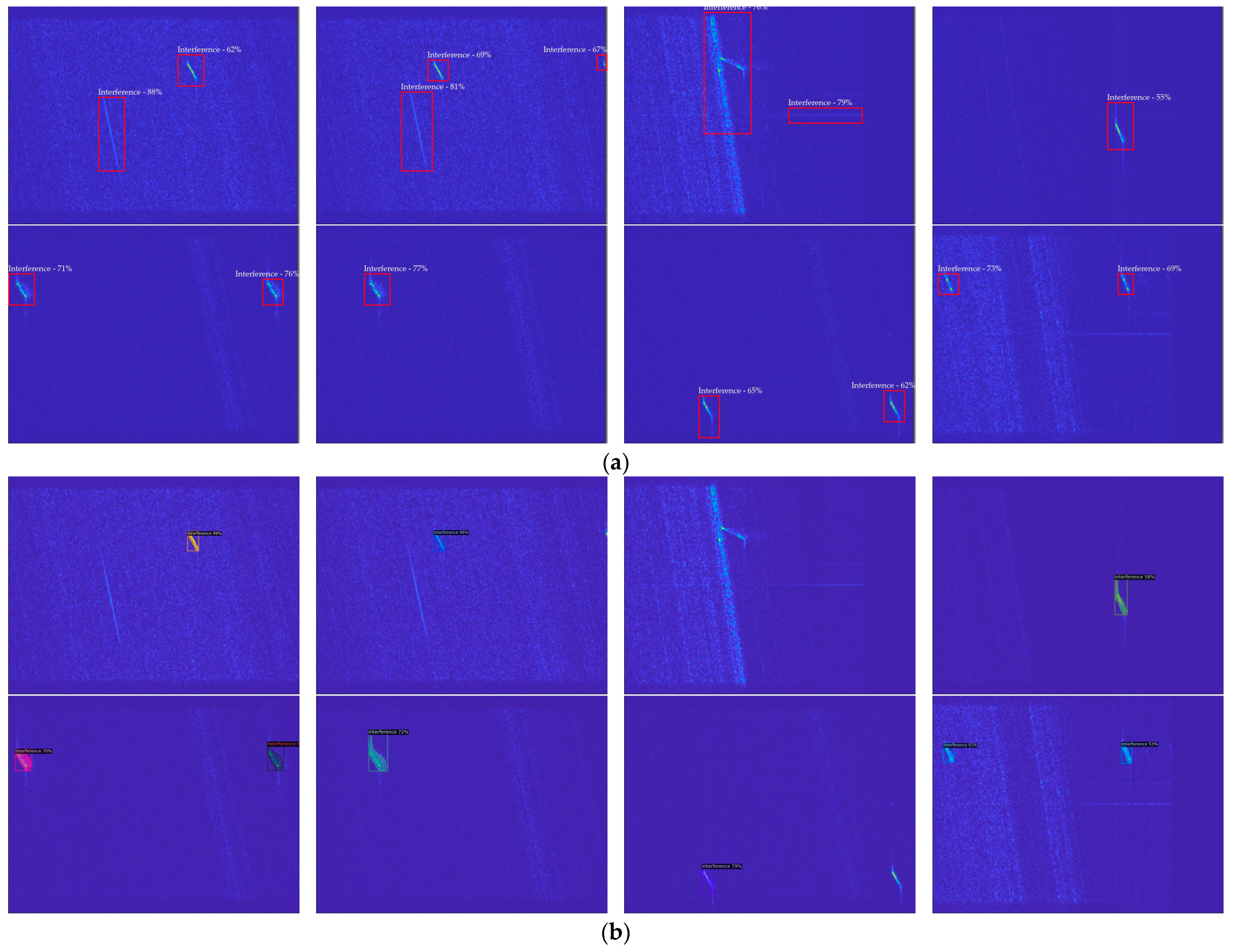
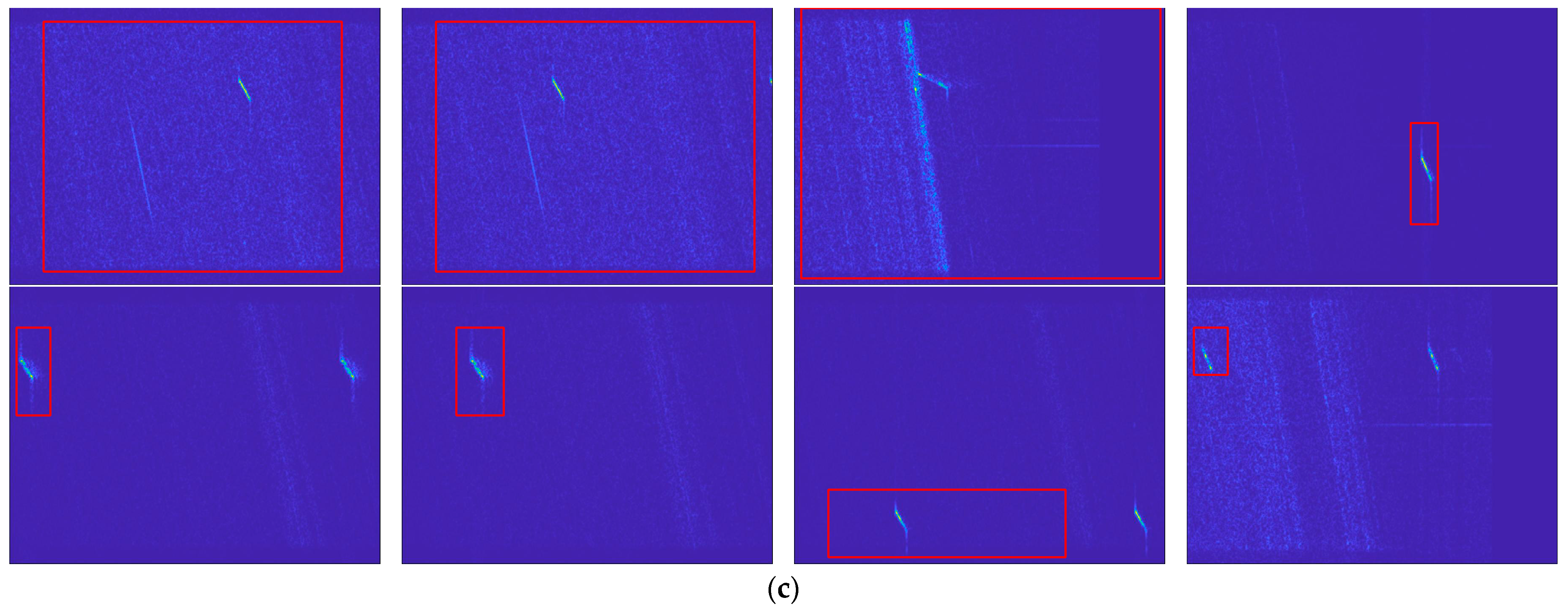
In this section, we use data without annotations to compare CEVIT, LOST [26], Cutler [28], and Tokencut [27] from different ISRs to show the detection results of the model proposed in this paper from the more intuitive visual detection results. Some of the test results are shown in Figure 11; the ISRs of the five time–frequency spectrograms are 5 dB, 5 dB, 6 dB, 8 dB, and 10 dB.
As shown in Figure 11, the ISR becomes gradually larger from left to right, i.e., the interference power is becoming larger and larger. The interference is selected by the red box or colored box in Figure 11, and it can be clearly seen that the detection performance of all the models increases with the increase in the ISR. In the case of complex interference, comparing (a) CEVIT, (b) Cutler [28], and (c) LOST [26], at a lower ISR, compared to the other two methods, CEVIT is able to detect more interfered regions in the time–frequency spectrograms and has fewer missed detections. Cutler tends to generate more false negatives, indicating it might miss some interference, while LOST struggles to produce robust detection results. As the ISR increases, CEVIT and Cutler perform quite similarly and can accurately detect interference. However, LOST’s performance is limited as it can only identify the location of the most prominent interference component in the image. The generated results and analysis may be attributed to the inclusion of the feature fusion module, which enables the model to focus more on global changes in the entire image rather than local variations. Additionally, the inclusion of the detection head module allows the model to represent the feature changes it captures as variations in interference power and type. Ultimately, this empowers the proposed model to excel in detecting interference under conditions of lower ISR and multiple types of interference. In contrast, Cutler’s self-training mechanism causes the model to depend more on previous detection results, resulting in a significant influence of previous results on the overall detection when the ISR is low. LOST, in its target localization process, selects the patch with the highest feature quantity as the seed and then searches the surroundings, making the detection results sensitive to the seed’s initial placement. As for the Tokencut method, it only selects the patch with the second smallest feature vector as the target when choosing feature quantities, limiting its ability to detect only a single interference source. However, it is notable that the model performs well in accurately locating the position of the most powerful interference.
Overall, CEVIT appears to offer a strong balance of performance across various ISR levels, making it an effective choice for interference detection in a complex interference environment.
4.3.2. Validation Set Detection Results
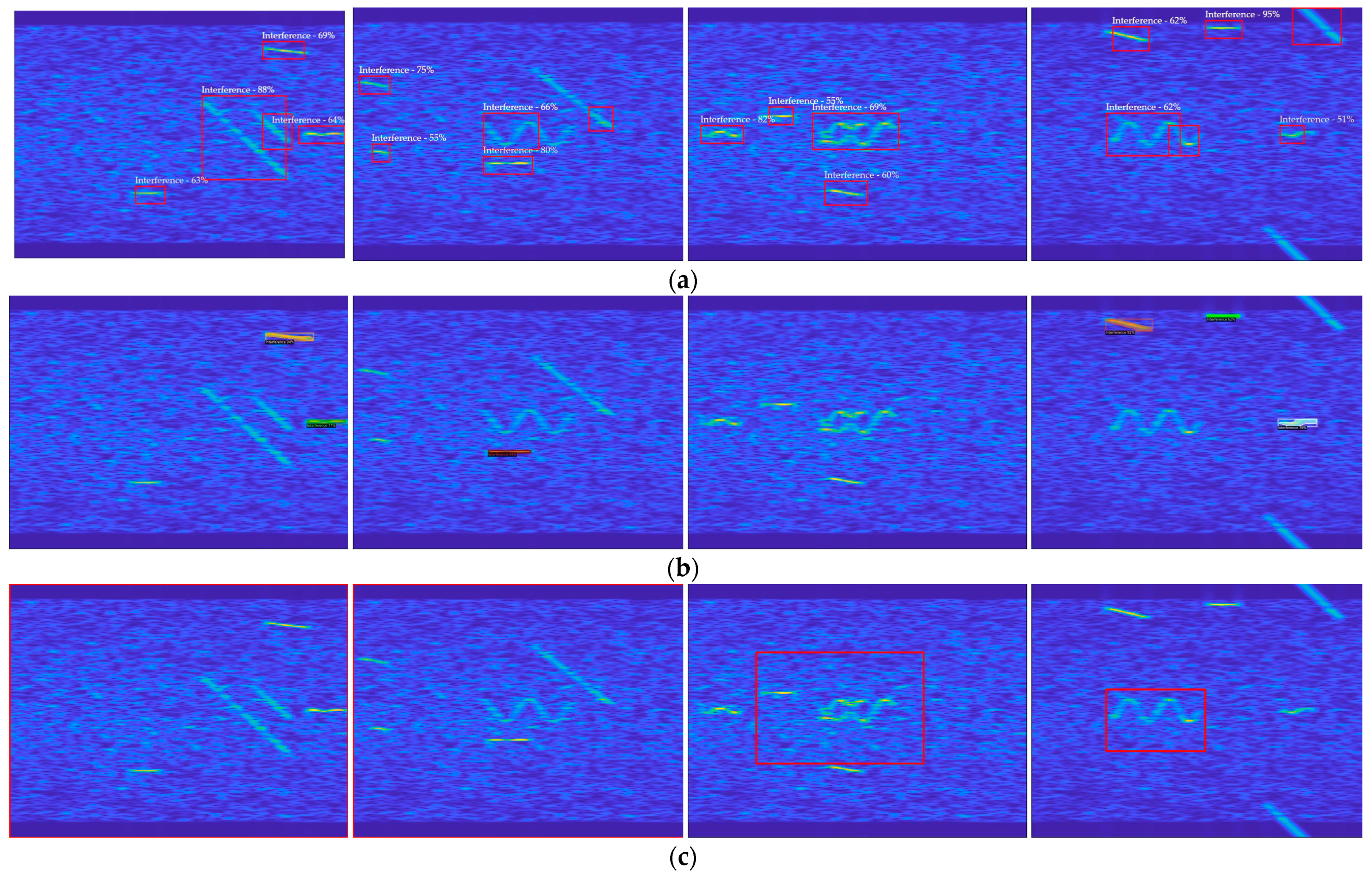
This section uses data containing annotation information to verify the performance of the proposed method in this paper in terms of evaluation indexes of the validation dataset, comparing CEVIT, Cutler, and LOST from the numerical results of the evaluation indexes and some of the experimental visualization results. The numerical results of the evaluation indexes and parts of the visualizations are shown in Table 3 and Figure 12. In Table 3, the best numerical results are bolded.
According to the table, the proposed model achieved the best results with a Recall of 0.7802 and an F1-score of 0.7871, demonstrating a significant improvement compared to the second-best performer. It obtained the second-best results in Precision and FPS, with a minor reduction compared to the top-performing Cutler.
In Figure 12, some visualized detection results are presented. Five randomly selected images from the validation set are used to compare the detection performance of the three methods. Interference is highlighted by red or colored boxes. It is evident that CEVIT can generate a higher number of detection boxes but with a slightly decreased precision in delineating the boundaries of interference. Cutler exhibits high accuracy in interference detection but may produce some false negatives. LOST can effectively detect strong interference in a high ISR but falls short in complex interference detection. In terms of overall detection performance, CEVIT results in fewer false negatives and excels in interference detection.
Comparing the three methods on real interfered Sentinel-1 echo data, the numerical results of the evaluation indexes and visualization results are shown in Table 4 and Figure 13. In Table 4, the best results are bolded.
It is evident that the Cutler model achieves the highest accuracy and detection speed, while the proposed model in this paper outperforms in terms of Recall and F1-score. This analysis can be attributed to the fact that the Cutler model places a high emphasis on accuracy requirements and is designed for object detection in natural images. This design leads the model to focus more on global features rather than local pixel variations, resulting in faster image detection but potentially leading to false negatives for low-power interference. In contrast, the proposed model attempts to perform feature-based searches on the feature map, utilizing edge detection within the detection head. This approach pays attention to pixel transition positions while introducing a relatively smaller computational overhead. As a result, it detects more interference without significantly compromising accuracy and detection speed, leading to noticeable improvements in Recall and F1-score. Some visualized detection results are presented in Figure 13.
5. Discussion
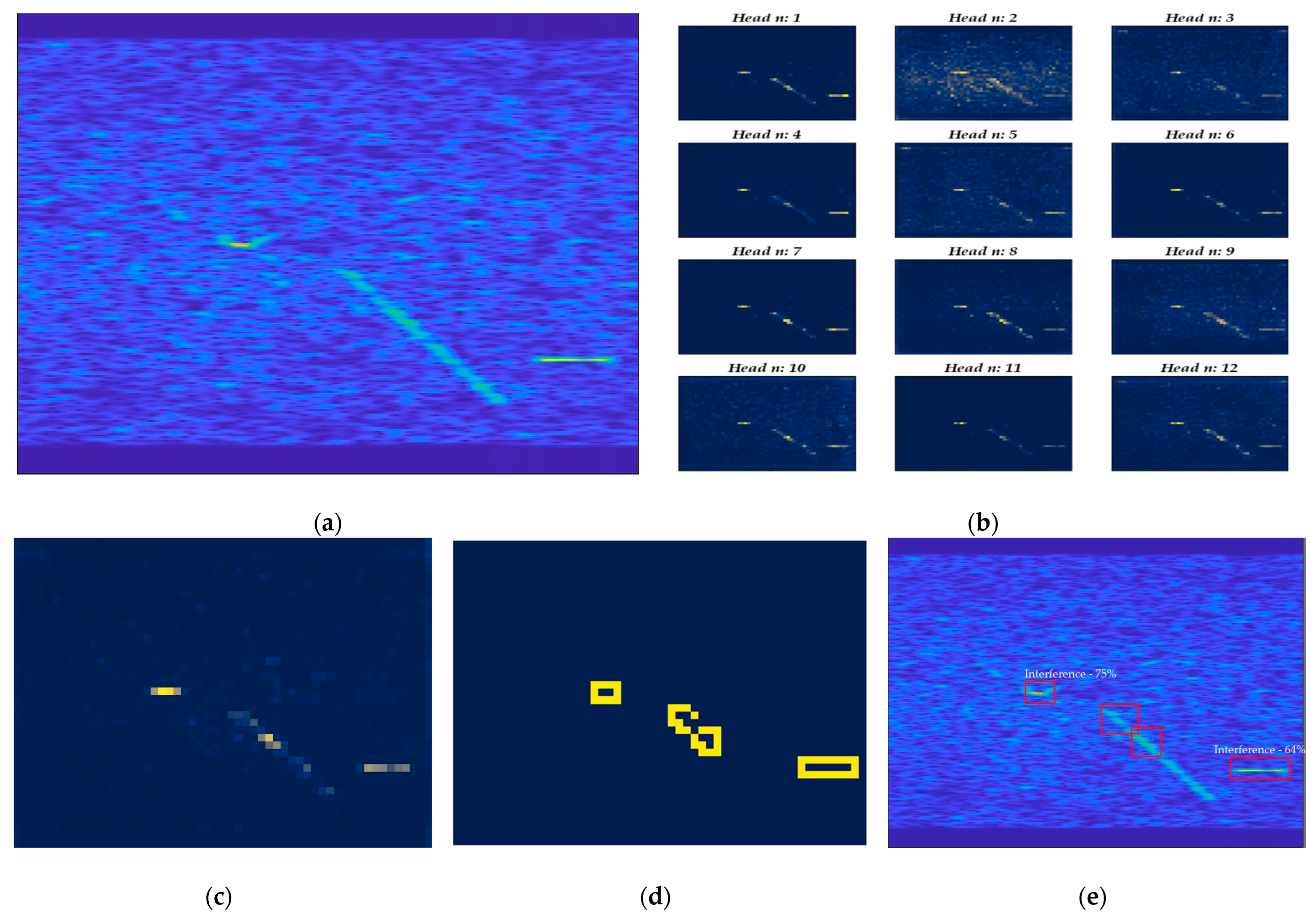
Although the proposed model shows a significant improvement in overall detection performance, we notice that, at a lower ISR, the model tends to produce more false alarms, especially for wideband interference, leading to a noticeable drop in accuracy. In Figure 14, we present a set consisting of an interfered time–frequency spectrogram, a feature map, an edge detection map, and the detection result.
The different colors in Figure 14c indicate the level of attention of the model, with higher highlighting indicating a higher level of attention. The yellow frames in Figure 14d indicate the result after edge detection. The red frames in Figure 14e indicate the result of detection The inclusion of narrowband sinusoidal interference, wideband chirp interference, and single-frequency interference can be clearly seen in the time–frequency spectrogram, while, in the attentional characterization plot, clear narrowband sinusoidal and point frequency interference can be noted, but a weaker characterization of the wideband chirp leads to its identification as multiple targets in the subsequent processing of the detector head module. Also, based on our experiments, the presence of such a problem for the interference of the wideband sin modulation is also noted. We judge that the reason for this problem is that the energy of the wideband signal tends to be evenly distributed within the bandwidth, which makes the interference power weaker compared to the narrowband signal, thus leading to the obvious parts of the extracted features. We note that, in the multi-head attention map, each attention head pays different attention to different types of interference, and the feature fusion block used in this paper only adopts the sum mean approach in fusing multi-head attention features, which lacks the targeted extraction of interference characteristics for each type of interference and thus results in the power of the extracted narrowband signal being higher than that of the wideband signal. In subsequent work, we will design and optimize the optimal weighted feature fusion block from the characteristics of interference types, weight the output of the attention of different heads, and realize the optimal extraction of features so as to reduce the false detection rate.
6. Conclusions
In this paper, an unsupervised SAR interference detection network based on a transformer and edge detection is proposed. The whole network consists of a feature extraction block, a feature fusion block, and a detection head module. By transforming the received echoes into the time–frequency domain, the time–frequency spectrogram is used as the input of the network; the pre-trained transformer is used as the backbone network to extract features; the multi-attention features are fused through the feature fusion block and fed into the detection head module; and the time–frequency spectrogram interference detection results are generated using Canny edge detection combined with the detection box generation strategy. Experiments on an airborne SAR simulation dataset and Sentinel-1 real interference echo data show that the method can obtain better detection results for many types of interference under a complex interference environment, and the detection consumes less time while obtaining good detection results. The Recall and F1-score improve by nearly 20%. The detection results on Sentinel-1 real interference echo data are the best results compared to those of other methods (Recall reaches 0.8722 and F1-score reaches 0.9115). The proposed method in this paper provides a new way and idea for real-time detection of interference in SAR systems.
However, the method proposed in this paper still has shortcomings, with more missed detections of wideband interference at a lower ISR. We will consider the characteristics of different interference, and our subsequent work will be centered around an optimally weighted feature fusion block and will attempt to lighten the model to maintain a faster detection speed while improving the detection accuracy.
Author Contributions
Conceptualization, Y.F. and X.G.; methodology, Y.F.; software, Y.F.; validation, Y.F., B.H. and X.W.; formal analysis, Y.F., J.S. and B.H.; investigation, Y.F.; resources, Y.F. and J.S.; data curation, Y.F.; writing—original draft preparation, Y.F., B.H., J.S. and X.W.; writing—review and editing, Y.F., B.H., J.S., X.G., H.D. and X.W.; visualization, Y.F.; supervision, B.H. and X.W.; project administration, B.H.; funding acquisition, B.H. and X.G. All authors have read and agreed to the published version of the manuscript.
Funding
This research was funded by National Natural Science Foundation of China (no. 62131019 and no. 41976169).
Data Availability Statement
The dataset and code used in this paper can be found on this website: https://github.com/yugangf/CEVIT (accessed on 20 December 2023).
Conflicts of Interest
The authors declare no conflicts of interest.
References
- Yan, H.; Bo, Z.; Mingliang, T.; Zhanye, C.; Wei, H. Review of synthetic aperture radar interference suppression. J. Radars 2020, 9, 86–106. [Google Scholar]
- Leng, X.; Ji, K.; Kuang, G. Radio frequency interference detection and localization in Sentinel-1 images. IEEE Trans. Geosci. Remote Sens. 2021, 59, 9270–9281. [Google Scholar] [CrossRef]
- Ma, B.; Yang, H.; Yang, J. Ship Detection in Spaceborne SAR Images under Radio Interference Environment Based on CFAR. Electronics 2022, 11, 4135. [Google Scholar] [CrossRef]
- Yang, Z.; Du, W.; Liu, Z.; Liao, G. WBI suppression for SAR using iterative adaptive method. IEEE J. Sel. Top. Appl. Earth Obs. Remote Sens. 2015, 9, 1008–1014. [Google Scholar] [CrossRef]
- Su, J.; Tao, H.; Tao, M.; Wang, L.; Xie, J. Narrow-band interference suppression via RPCA-based signal separation in time– frequency domain. IEEE J. Sel. Top. Appl. Earth Obs. Remote Sens. 2017, 10, 5016–5025. [Google Scholar] [CrossRef]
- Li, N.; Zhang, H.; Lv, Z.; Min, L.; Guo, Z. Simultaneous screening and detection of RFI from massive SAR images: A case study on European Sentinel-1. IEEE Trans. Geosci. Remote Sens. 2022, 60, 1–17. [Google Scholar] [CrossRef]
- Tao, M.; Zhou, F.; Zhang, Z. Wideband interference mitigation in high-resolution airborne synthetic aperture radar data. IEEE Trans. Geosci. Remote Sens. 2015, 54, 74–87. [Google Scholar] [CrossRef]
- Wang, X.Y.; Yu, W.D.; Qi, X.Y.; Liu, Y. RFI suppression in SAR based on approximated spectral decomposition algorithm. Electron. Lett. 2012, 48, 594–596. [Google Scholar] [CrossRef]
- Natsuaki, R.; Motohka, T.; Watanabe, M.; Shimada, M.; Suzuki, S. An autocorrelation-based radio frequency interference detection and removal method in azimuth-frequency domain for SAR image. IEEE J. Sel. Top. Appl. Earth Obs. Remote Sens. 2017, 10, 5736–5751. [Google Scholar] [CrossRef]
- Xian, S.; Yu, M.; WenHui, D.; Lijia, H.; Xin, Z.; Jiancheng, L.; Lianru, G.; Peijin, W.; Zhiyuan, Y.; Lijing, G.; et al. The review of AI-based intelligent remote sensing capabilities. J. Image Graph. 2022, 27, 1799–1822. [Google Scholar]
- Yu, J.; Li, J.; Sun, B.; Chen, J.; Li, C. Multiclass radio frequency interference detection and suppression for SAR based on the single shot multibox detector. Sensors 2018, 18, 4034. [Google Scholar] [CrossRef]
- Lv, Q.; Quan, Y.; Feng, W.; Sha, M.; Dong, S.; Xing, M. Radar deception jamming recognition based on weighted ensemble CNN with transfer learning. IEEE Trans. Geosci. Remote Sens. 2021, 60, 1–11. [Google Scholar] [CrossRef]
- Chojka, A.; Artiemjew, P.; Rapiński, J. RFI artefacts detection in Sentinel-1 level-1 SLC data based on image processing techniques. Sensors 2020, 20, 2919. [Google Scholar] [CrossRef] [PubMed]
- Junfei, Y.; Jingwen, L.; Bing, S.; Yuming, J. Barrage jamming detection and classification based on convolutional neural network for synthetic aperture radar. In Proceedings of the IGARSS 2018—2018 IEEE International Geoscience and Remote Sensing Symposium, Valencia, Spain, 22–27 July 2018; pp. 4583–4586. [Google Scholar]
- Shen, J.; Han, B.; Pan, Z.; Li, G.; Hu, Y.; Ding, C. Learning time–frequency information with prior for SAR radio frequency interference suppression. IEEE Trans. Geosci. Remote Sens. 2022, 60, 1–16. [Google Scholar] [CrossRef]
- Tao, M.; Li, J.; Chen, J.; Liu, Y.; Fan, Y.; Su, J.; Wang, L. Radio frequency interference signature detection in radar remote sensing image using semantic cognition enhancement network. IEEE Trans. Geosci. Remote Sens. 2022, 60, 1–14. [Google Scholar] [CrossRef]
- Liu, Y.; Zhang, Y.; Wang, Y.; Hou, F.; Yuan, J.; Tian, J.; Zhang, Y.; Shi, Z.; Fan, J.; He, Z. A survey of visual transformers. IEEE Trans. Neural Netw. Learn. Syst. 2023, 1–21. [Google Scholar] [CrossRef]
- Dosovitskiy, A.; Beyer, L.; Kolesnikov, A.; Weissenborn, D.; Zhai, X.; Unterthiner, T.; Dehghani, M.; Minderer, M.; Heigold, G.; Gelly, S.; et al. An image is worth 16 × 16 words: Transformers for image recognition at scale. arXiv 2020, arXiv:2010.11929. [Google Scholar]
- Carion, N.; Massa, F.; Synnaeve, G.; Usunier, N.; Kirillov, A.; Zagoruyko, S. End-to-end object detection with transformers. In Proceedings of the European Conference on Computer Vision; Springer: Cham, Switzerland, 2020; pp. 213–229. [Google Scholar]
- Jain, J.; Li, J.; Chiu, M.T.; Hassani, A.; Orlov, N.; Shi, H. Oneformer: One transformer to rule universal image segmentation. In Proceedings of the IEEE/CVF Conference on Computer Vision and Pattern Recognition, Vancouver, BC, Canada, 18–22 June 2023; pp. 2989–2998. [Google Scholar]
- Zong, Z.; Song, G.; Liu, Y. Detrs with collaborative hybrid assignments training. In Proceedings of the IEEE/CVF International Conference on Computer Vision, Paris, France, 2–3 October 2023; pp. 6748–6758. [Google Scholar]
- Zhu, X.; Su, W.; Lu, L.; Li, B.; Wang, X.; Dai, J. Deformable detr: Deformable transformers for end-to-end object detection. arXiv 2020, arXiv:2010.04159. [Google Scholar]
- He, K.; Chen, X.; Xie, S.; Li, Y.; Dollár, P.; Girshick, R. Masked autoencoders are scalable vision learners. In Proceedings of the IEEE/CVF Conference on Computer Vision and Pattern Recognition, New Orleans, LA, USA, 18–24 June 2022; pp. 16000–16009. [Google Scholar]
- Zhang, H.; Li, F.; Liu, S.; Zhang, L.; Su, H.; Zhu, J.; Ni, L.M.; Shum, H.Y. Dino: Detr with improved denoising anchor boxes for end-to-end object detection. arXiv 2022, arXiv:2203.03605. [Google Scholar]
- Caron, M.; Touvron, H.; Misra, I.; Jégou, H.; Mairal, J.; Bojanowski, P.; Joulin, A. Emerging properties in self-supervised vision transformers. In Proceedings of the IEEE/CVF International Conference on Computer Vision, Montreal, BC, Canada, 11–17 October 2021; pp. 9650–9660. [Google Scholar]
- Siméoni, O.; Puy, G.; Vo, H.V.; Roburin, S.; Gidaris, S.; Bursuc, A.; Pérez, P.; Marlet, R.; Ponce, J. Localizing objects with self-supervised transformers and no labels. arXiv 2021, arXiv:2109.14279. [Google Scholar]
- Wang, Y.; Shen, X.; Yuan, Y.; Du, Y.; Li, M.; Hu, S.X.; Crowley, J.L.; Vaufreydaz, D. Tokencut: Segmenting objects in images and videos with self-supervised transformer and normalized cut. arXiv 2022, arXiv:2209.00383. [Google Scholar] [CrossRef] [PubMed]
- Wang, X.; Girdhar, R.; Yu, S.X.; Misra, I. Cut and learn for unsupervised object detection and instance segmentation. In Proceedings of the IEEE/CVF Conference on Computer Vision and Pattern Recognition, Vancouver, BC, Canada, 18–22 June 2023; pp. 3124–3134. [Google Scholar]
- Ren, S.; He, K.; Girshick, R.; Sun, J. Faster r-cnn: Towards real-time object detection with region proposal networks. Adv. Neural Inf. Process. Syst. 2015, 28. [Google Scholar] [CrossRef] [PubMed]
- Lin, T.Y.; Dollár, P.; Girshick, R.; He, K.; Hariharan, B.; Belongie, S. Feature pyramid networks for object detection. In Proceedings of the IEEE Conference on Computer Vision and Pattern Recognition, Honolulu, HI, USA, 21–26 July 2017; pp. 2117–2125. [Google Scholar]
- Liu, W.; Anguelov, D.; Erhan, D.; Szegedy, C.; Reed, S.; Fu, C.Y.; Berg, A.C. Ssd: Single shot multibox detector. In Proceedings of the Computer Vision–ECCV 2016: 14th European Conference, Amsterdam, The Netherlands, 11–14 October 2016; pp. 21–37. [Google Scholar]
- Ba, J.L.; Kiros, J.R.; Hinton, G.E. Layer normalization. arXiv 2016, arXiv:1607.06450. [Google Scholar]
- Vaswani, A.; Shazeer, N.; Parmar, N.; Uszkoreit, J.; Jones, L.; Gomez, A.N.; Kaiser, Ł.; Polosukhin, I. Attention is all you need. Adv. Neural Inf. Process. Syst. 2017, 30. [Google Scholar]
- Canny, J. A computational approach to edge detection. IEEE Trans. Pattern Anal. Mach. Intell. 1986, PAMI-8, 679–698. [Google Scholar] [CrossRef]
- Neubeck, A.; Van Gool, L. Efficient non-maximum suppression. In Proceedings of the 18th International Conference on Pattern Recognition (ICPR’06), Hong Kong, China, 20–24 August 2006; Volume 3, pp. 850–855. [Google Scholar]
- Liu, Y.Q.; Du, X.; Shen, H.L.; Chen, S.J. Estimating generalized gaussian blur kernels for out-of-focus image deblurring. IEEE Trans. Circuits Syst. Video Technol. 2020, 31, 829–843. [Google Scholar] [CrossRef]
- Gedraite, E.S.; Hadad, M. Investigation on the effect of a Gaussian Blur in image filtering and segmentation. In Proceedings of the ELMAR-2011, Zadar, Croatia, 14–16 September 2011; pp. 393–396. [Google Scholar]
Figure 1.
Frequency domain analysis and time–frequency domain analysis results for different interference. (a) Frequency domain analysis and time–frequency domain analysis results of single-frequency interference; (b) frequency domain analysis and time–frequency domain analysis results of narrowband chirp-modulated interference; (c) frequency domain analysis and time–frequency domain analysis results of wideband chirp-modulated interference; (d) frequency domain analysis and time–frequency domain analysis results of narrowband sinusoidal-modulated interference; (e) frequency domain analysis and time–frequency domain analysis results of wideband sinusoidal-modulated interference.


Figure 2.
Frequency domain and time–frequency analysis results for lower-ISR complex interference. (a) Frequency domain analysis results of lower-ISR complex interference; (b) time–frequency analysis results of lower-ISR complex interference.
Figure 2.
Frequency domain and time–frequency analysis results for lower-ISR complex interference. (a) Frequency domain analysis results of lower-ISR complex interference; (b) time–frequency analysis results of lower-ISR complex interference.

Figure 3.
Frequency domain and time–frequency analysis results for higher-ISR complex interference. (a) Frequency domain analysis results of higher-ISR complex interference; (b) time–frequency analysis results of higher-ISR complex interference.
Figure 3.
Frequency domain and time–frequency analysis results for higher-ISR complex interference. (a) Frequency domain analysis results of higher-ISR complex interference; (b) time–frequency analysis results of higher-ISR complex interference.

Figure 4.
Overview of the complete processing pipeline of CEVIT.

Figure 5.
Input image and multi-head attention maps. (a) Input image; (b) multi-head attention maps.
Figure 5.
Input image and multi-head attention maps. (a) Input image; (b) multi-head attention maps.

Figure 6.
The results of the comparison between a single feature (K feature, for example) and the fused features. (a) Single feature map (K feature, for example); (b) fused feature map.
Figure 6.
The results of the comparison between a single feature (K feature, for example) and the fused features. (a) Single feature map (K feature, for example); (b) fused feature map.

Figure 7.
Examples of the time–frequency spectrograms and the pixel value cumulative distribution function of the spectrograms. (a) Time–frequency spectrograms; (b) the pixel value distribution function of spectrograms.
Figure 7.
Examples of the time–frequency spectrograms and the pixel value cumulative distribution function of the spectrograms. (a) Time–frequency spectrograms; (b) the pixel value distribution function of spectrograms.

Figure 8.
The imaging result and original time–frequency spectrogram of the raw echo data of the airborne SAR. (a) Imaging result of airborne SAR; (b) time–frequency spectrogram of airborne SAR.
Figure 8.
The imaging result and original time–frequency spectrogram of the raw echo data of the airborne SAR. (a) Imaging result of airborne SAR; (b) time–frequency spectrogram of airborne SAR.

Figure 9.
Examples of the time–frequency spectrograms and imaging results of the interfered echoes. Dashed frame of different colors indicates different interference in the image. (a) Time–frequency spectrograms; (b) imaging results.
Figure 9.
Examples of the time–frequency spectrograms and imaging results of the interfered echoes. Dashed frame of different colors indicates different interference in the image. (a) Time–frequency spectrograms; (b) imaging results.


Figure 10.
The interfered image domain and echo domain of Sentinel-1. (a) Interfered image domain of Sentinel-1; (b) overall interfered echoes of Sentinel-1.
Figure 10.
The interfered image domain and echo domain of Sentinel-1. (a) Interfered image domain of Sentinel-1; (b) overall interfered echoes of Sentinel-1.

Figure 11.
Detection results of four models with different ISRs: (a) CEVIT (the red frame in the figure marks the detection result); (b) Cutler (different colored frames and masks indicate detection results); (c) LOST (the red frame in the figure marks the detection result). (d) Tokencut.
Figure 11.
Detection results of four models with different ISRs: (a) CEVIT (the red frame in the figure marks the detection result); (b) Cutler (different colored frames and masks indicate detection results); (c) LOST (the red frame in the figure marks the detection result). (d) Tokencut.


Figure 12.
Visualization of detection results for three methods’ validation sets. (a) CEVIT (the red frame in the figure marks the detection result); (b) Cutler (different colored frames and masks indicate detection results); (c) LOST (the red frame in the figure marks the detection result).
Figure 12.
Visualization of detection results for three methods’ validation sets. (a) CEVIT (the red frame in the figure marks the detection result); (b) Cutler (different colored frames and masks indicate detection results); (c) LOST (the red frame in the figure marks the detection result).

Figure 13.
Visualization of detection results for three methods in Sentinel-1 data. (a) CEVIT (the red frame in the figure marks the detection result); (b) Cutler (different colored frames and masks indicate detection results); (c) LOST (the red frame in the figure marks the detection result).
Figure 13.
Visualization of detection results for three methods in Sentinel-1 data. (a) CEVIT (the red frame in the figure marks the detection result); (b) Cutler (different colored frames and masks indicate detection results); (c) LOST (the red frame in the figure marks the detection result).


Figure 14.
A set consisting of interfered time–frequency spectrogram, multi-head attention map, feature map, edge detection map, and detection result. (a) Time–frequency spectrogram; (b) multi-head attention map; (c) feature map; (d) edge detection map; (e) detection result.
Figure 14.
A set consisting of interfered time–frequency spectrogram, multi-head attention map, feature map, edge detection map, and detection result. (a) Time–frequency spectrogram; (b) multi-head attention map; (c) feature map; (d) edge detection map; (e) detection result.


Table 1.
Basic parameters of two kinds of SAR echoes used in simulation and experiments.
| Attribute | Airborne SAR Echoes | Sentinel-1 Echoes |
|---|---|---|
| Wave Length (m) | ||
| Chirp Rate (Hz/s) | −2 × 10¹⁴ | 1.1 × 10¹² |
| Pulse Width (s) | 2.4 × 10⁻⁶ | 5.24 × 10⁻⁵ |
| Range Sample Rate (MHz) | ||
| Velocity (m/s) | ||
| Prf (Hz) |
Table 2.
Interference type and basic parameters.
| Interference Type | Parameters | Values |
|---|---|---|
| Numbers | ||
| Bandwidth | MHz | |
| Chirp Rate | ||
| Numbers | ||
| Bandwidth | MHz | |
| Chirp Rate | ||
| Numbers | ||
| Bandwidth | MHz | |
| Modulation Coefficient | ||
| Initial Phase | ||
| Numbers | ||
| Bandwidth | MHz | |
| Modulation Coefficient | ||
| Initial Phase | ||
| Numbers |
Disclaimer/Publisher’s Note: The statements, opinions and data contained in all publications are solely those of the individual author(s) and contributor(s) and not of MDPI and/or the editor(s). MDPI and/or the editor(s) disclaim responsibility for any injury to people or property resulting from any ideas, methods, instructions or products referred to in the content. |
© 2024 by the authors. Licensee MDPI, Basel, Switzerland. This article is an open access article distributed under the terms and conditions of the Creative Commons Attribution (CC BY) license (https://creativecommons.org/licenses/by/4.0/).
Share and Cite
MDPI and ACS Style
Feng, Y.; Han, B.; Wang, X.; Shen, J.; Guan, X.; Ding, H. Self-Supervised Transformers for Unsupervised SAR Complex Interference Detection Using Canny Edge Detector. Remote Sens. 2024, 16, 306. https://doi.org/10.3390/rs16020306
AMA Style
Feng Y, Han B, Wang X, Shen J, Guan X, Ding H. Self-Supervised Transformers for Unsupervised SAR Complex Interference Detection Using Canny Edge Detector. Remote Sensing. 2024; 16(2):306. https://doi.org/10.3390/rs16020306
Chicago/Turabian StyleFeng, Yugang, Bing Han, Xiaochen Wang, Jiayuan Shen, Xin Guan, and Hao Ding. 2024. "Self-Supervised Transformers for Unsupervised SAR Complex Interference Detection Using Canny Edge Detector" Remote Sensing 16, no. 2: 306. https://doi.org/10.3390/rs16020306
Note that from the first issue of 2016, this journal uses article numbers instead of page numbers. See further details here.