

Impact Analysis of Satellite Geometry Variation on ARAIM Integrity Risk over Exposure Interval
College of Intelligent System Science and Engineering, Harbin Engineering University, Harbin 150001, China
*
Author to whom correspondence should be addressed.
Remote Sens. 2024, 16(2), 286; https://doi.org/10.3390/rs16020286
Submission received: 19 October 2023
/
Revised: 5 January 2024
/
Accepted: 8 January 2024
/
Published: 10 January 2024
(This article belongs to the Special Issue Advanced Technologies for Position and Navigation under GNSS Signal Challenging or Denied Environments III)
Abstract
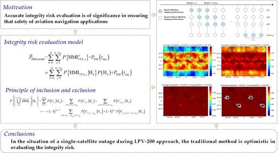
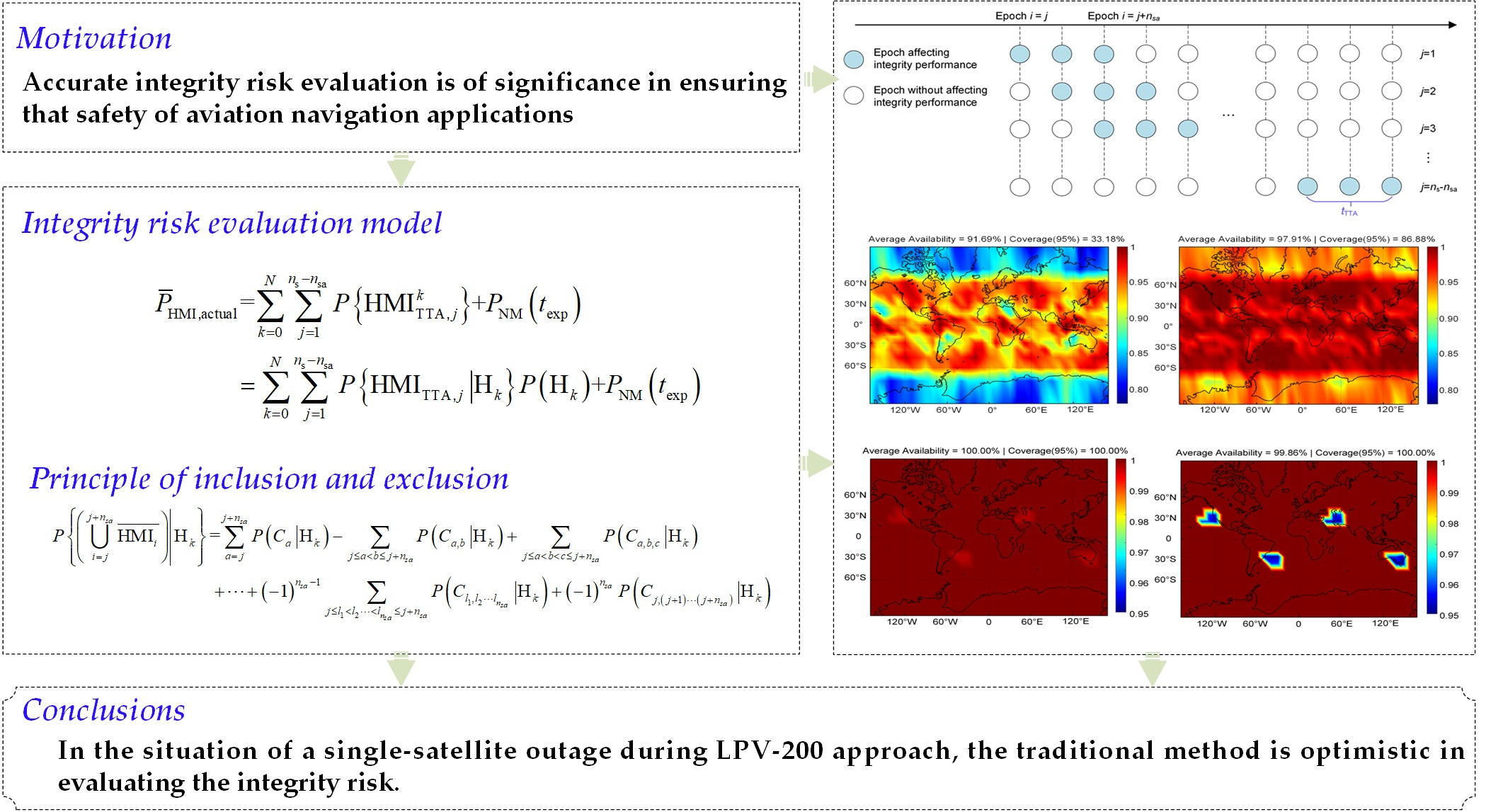
:Accurate integrity risk evaluation is of significance in ensuring that aviation navigation applications satisfy the predefined integrity requirement. The integrity risk evaluation method over a specified exposure interval has been proposed in previous works for the development of advanced receiver autonomous integrity monitoring (ARAIM) (ARAIM technical subgroup reference airborne algorithm description document v4.1, 2022). However, this method typically relies on an underlying optimistic assumption that the satellite geometry remains constant throughout the exposure interval. The variation in satellite geometry due to potential satellite outages undermines the widely-used geometry constant assumption. Thus, we investigate the influence of satellite geometry variations throughout the exposure interval on the integrity performance by introducing a geometry-sensitive risk-evaluation model. The findings demonstrate that, under the nominal situation, the region where the ARAIM fails to meet predefined integrity requirement could expand by a maximum of 2.93% when accounting for satellite geometry variations. Furthermore, in the situation of a single satellite outage, this hazardous region has significantly expanded from 13.12% of the global coverage to 66.82%. Based on these findings, we recommend that the ARAIM should consider satellite outages as a critical factor in real-time integrity risk evaluation.
1. Introduction
The global navigation satellite system (GNSS)-based positioning service is susceptible to rare faults, such as satellite and constellation faults, which can threaten the integrity of aircraft navigation [1,2]. Receiver autonomous integrity monitoring (RAIM) and Advanced RAIM (ARAIM) have been developed to support the integrity of positioning. The classic RAIM algorithm is designed to satisfy the required navigation performance (RNP) of en-route and non-precision approach phases as defined by the international civil aviation organization [3]. With the full deployment of the Galileo and Beidou navigation satellite system (BDS), an increased number of redundant observations are available [4,5,6]. There has been a renewed interest in expanding the RAIM to satisfy more demanding RNP, such as with the localizer precision vertical 200 (LPV-200) [7].
With this goal, the Global Positioning System (GPS) Evolutionary Architecture Study (GEAS) introduced a new concept of dual-frequency multi-constellation ARAIM and a corresponding user algorithm [8]. One of the primary tasks in ARAIM is to evaluate the integrity risk, or alternatively, a protection level, which is an upper bound on the positioning error with a specified integrity requirement. According to the definition of the international civil aviation organization (ICAO), integrity risk refers to the probability of a positioning error exceeding the specified alarm limit throughout the exposure interval, while the system fails to provide a timely warning to the user [9,10]. The exposure interval corresponds to the period of navigation service. For instance, the exposure interval for the LPV-200 is set at 150 s. Integrity risk evaluation is needed when designing a navigation system to meet a predefined integrity requirement PHMI,REQ, and it is needed operationally to inform the user whether to abort or to pursue a mission [11]. In most of the literature [11,12,13], the integrity risk is evaluated at a single epoch without considering detection across multiple epochs, even though their corresponding requirements are specified over the exposure interval [14]. The literature assumes that when the correlation times of detection statistics and positioning error are significantly greater than the exposure interval, the integrity risk would be nearly constant as if one independent test was executed over the interval [14]. However, there has been some relevant earlier work on ARAIM suggesting that the assumption is not true, and that the actual integrity risk can be much higher [14,15]. To resolve these issues, Milner et al. [15] and Blanch et al. [16] proposed an integrity risk evaluation method that accurately accounts for the time-correlation effect of detection statistics and positioning error by utilizing the number of effective samples (NES). The NES represents the ratio of the integrity risk for a single epoch to the integrity risk over an exposure interval, and it can be computed using a first-order Gauss Markov model. When determining the NES, the upper limit of integrity risk over a given exposure interval can be evaluated based on the integrity risk observed at a single epoch within that interval [17]. At present, this algorithm has been adopted in the ARAIM technical subgroup reference airborne algorithm-description document [1]. However, to simplify the complexity of integrity risk evaluation, this method typically assumes a constant satellite geometry throughout the exposure interval. Unfortunately, the variation in satellite geometry is frequent and presents practical challenges for accurate integrity risk evaluation. This traditional assumption can introduce errors in integrity risk evaluation, particularly as the exposure interval increases. Therefore, we focus on the integrity risk evaluation of ARAIM in the presence of satellite geometry variation in this contribution.
Currently, the integrity risk evaluation based on the NES generally assumes a constant satellite geometry throughout the exposure interval. This assumption is regarded as reasonable only under the following conditions: First, the duration of the given exposure interval should be short. For instance, this assumption can be applicable to an LPV-200 approach with an exposure interval of 150 s. Secondly, there should be no satellite outages throughout the exposure interval. Unfortunately, achieving both of these conditions simultaneously is often challenging in real-time aviation navigation applications. There are several factors that can cause satellite outages within the exposure interval, e.g., aircraft banking and ionospheric scintillation. The aircraft attitude affects the reception of the signal because the antenna pattern is such that signals coming from underneath the plane of the aircraft suffer a significant loss of power [18]. Outages can also occur due to ionospheric scintillation, particularly in low latitude regions, which are affected by the equatorial anomaly. The addition or removal of a satellite in the view, especially for weak geometries, can cause significant changes in the satellite geometry. This variation in satellite geometry undermines the widely-used assumption of constant geometry and can result in errors in integrity risk evaluation. Although the ARAIM algorithm incorporates multiple conservative assumptions to constrain the actual integrity risk, to our knowledge, there is a lack of prior studies investigating the influence of satellite geometry variations within the exposure interval on the performance of the NES-based ARAIM. Nikiforov [19] has conducted a simulation analysis in previous research to quantify satellite geometry variations within the exposure interval. However, these quantitative results were primarily focused on a shorter exposure interval, and the impact of satellite geometry variations on integrity risk was not further explored. For this purpose, we investigate the actual integrity performance of the ARAIM under different situations of satellite geometry variation. If the observed performance significantly exceeds the predefined integrity risk requirement, it can provide a foundation for developing a more efficient integrity risk evaluation method to achieve better real-time performance.
According to the above analysis, the rigorous integrity risk-evaluation model is primarily constrained by the accurate description of satellite geometry variation within the exposure interval. Monte Carlo (MC) simulation is a straightforward, brute-force method employed to solve a complex model [20]. However, this approach is impractical for our performance verification due to its time-consuming nature, especially when considering worldwide integrity performance. An analytical integrity risk evaluation is more suitable for conducting worldwide performance verification. To the best of our knowledge, a rigorous integrity risk-evaluation model that considers satellite geometry variation within the exposure interval is still absent. In this contribution, we develop a general integrity risk-evaluation model to quantify the impact of satellite geometry variation on integrity performance. The principle of inclusion and exclusion (PIE) is introduced to rigorously characterize the influence of the satellite geometry variation within the exposure interval. It should be noted that our proposed method is designed for application in the offline integrity performance analysis of ARAIM. Through a rigorous assessment of ARAIM’s integrity performance, it is poised to furnish a dependable foundation for performance verification, as well as the subsequent update and adjustment of the ARAIM algorithm.
The next section introduces the concept of overall integrity risk to clarify the integrity requirements for ARAIM operations. In the following sections, we review the least-squares estimation of states of interest and the current ARAIM fault-detection algorithm to define the hazardously misleading information (HMI). The HMI definition will serve as a foundation for integrity risk evaluation. Next, we provide a detailed overview of the methodology we applied to evaluate the integrity risk of ARAIM. Following the detailed description of the method, we proceed to analyze the bounding tightness of the proposed method to the integrity risk reference, ensuring the effectiveness of the subsequent performance verification. Finally, we present the resulting integrity risk performance of the ARAIM under various simulation conditions, discuss the influence of satellite geometry variation on integrity performance, and concludes with remark on the future work.
2. Problem Definition
Since the integrity risk requirement is defined as the probability over the specific exposure interval, the integrity risk is required to evaluate over multiple detection epochs. Without losing generality, the integrity risk over the exposure interval can be expressed as [21],
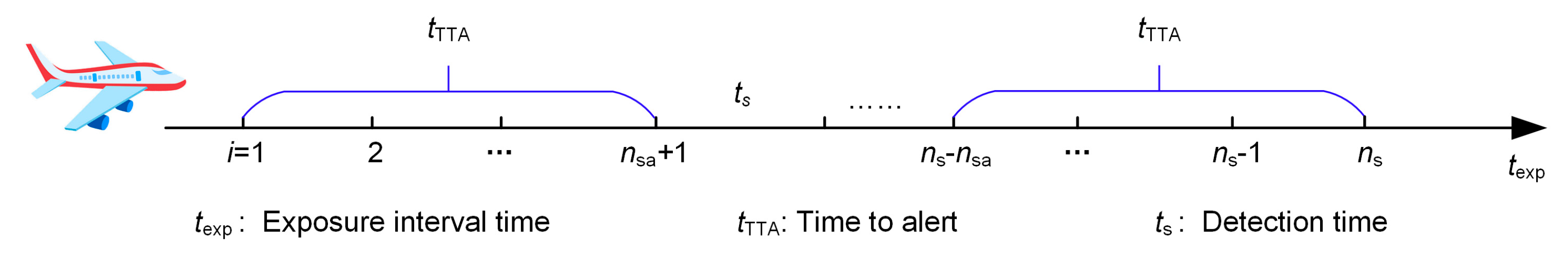
where HMI represents the hazardous misleading information, which is the situation when an undetected positioning error exceeds a predefined alert limit (AL). There are three different time metrics for integrity risk evaluation, i.e., the exposure interval time (texp), the time-to-alert (tTTA) defined by required navigation performance, and the single detection time (ts). Based on these time metrics, two parameters required for integrity risk evaluation, i.e., ns and nsa, can be determined. The ns is the number of epochs in the texp, i.e., texp/ts. The nsa is the number of epochs in the tTTA, i.e., tTTA/ts. As seen from Figure 1, we usually have texp > tTTA > ts. Furthermore, Hk in (1) represents the fault mode hypotheses for k = 0…N, which account for all fault satellite combinations including H0, single satellite fault, multi-satellite faults, and constellation fault [22,23,24,25]. N is the number of fault modes to be monitored. PNM(texp) is the probability of the fault modes that need not be monitored in the exposure interval. The calculation method of PNM(texp) and the fault modes number N can be found in [16]. i and j represent the epoch time within the exposure interval. It should be noted that we will denote the event of continuous HMI occurrence within tTTA under fault mode k, i.e., , as in the following to simplify the notation.
The integrity risk over the exposure interval can be accurately evaluated based on (1) [13]. However, the evaluation of integrity risk based on (1) is computationally challenged by the presence of time-correlation among multiple epochs [8]. A conservative but computationally efficient risk-evaluation model is usually used to calculate the integrity risk, instead of (1) [23],
where is the prior probability of the fault mode Hk. It should be noted that the subscript i of Hk,i is eliminated in (2) because we assume that the fault mode occurring at the first epoch in the exposure interval will always persist in this interval. This assumption is reasonable, because according to analysis in [1], the mean fault duration of GPS and Galileo is 1 h, which is usually much longer than the exposure interval. Equation (2) strictly considers all epochs’ geometry in the exposure interval and is referred to as the geometry-sensitive risk-evaluation model.
Provided the statistical distribution of HMI and the satellite geometry from all epochs across the exposure interval, the integrity risk can be obtained based on the geometry-sensitive risk-evaluation model. Nonetheless, it is usually difficult to forecast the satellite geometry variation in the exposure interval for real-time aviation navigation applications. Therefore, the geometry constant assumption within the exposure interval is adopted to simplify the complexity of integrity risk evaluation. However, the satellite geometry variation due to the rising and falling of satellites undermines the widely-used geometry constant assumption. This assumption may lead to an integrity risk-evaluation error. Next, we will introduce a general integrity risk-evaluation method to investigate the influence of satellite geometry variations throughout the exposure interval on the integrity performance of the NES-based ARAIM.
3. Integrity Risk Evaluation over the Exposure Interval
This section describes a general methodology for evaluating the integrity risk within the exposure interval. It begins by reviewing the definition of HMI events in the baseline ARAIM algorithm. Subsequently, the rigorous PHMI evaluation approach based on the geometry-sensitive model (2) is introduced.
3.1. Hazardous Misleading Information
This section provides a description of the HMI definition for various satellite geometry. According to (2), the integrity risk of navigation application is determined by the temporal characteristics of the HMI events. In the baseline ARAIM algorithm, the HMI event under fault mode hypotheses k is described as [17]
where is a position estimate error using all satellites in view at epoch i. The subscript q = 1, 2, and 3 denote the east, north, and up components, respectively. is a position estimate error using all satellites except the one(s) included in fault mode d. The distribution of in (3) and (4) can be written in detail as
where is a 1 × n project vector to exclude the fault satellite, i.e., , Rc is the identity matrix with the c-th diagonal element equal to 0 when the c-th satellite is included in fault mode hypothesis d, and eq is the m × 1 vector used to extract the q-th state out of the full state vector. For example, use of to extract the vertical position error. bnom is the n × 1 nominal bias vector. is the standard deviation of the estimated error for the q-th state. Hi is the n × m normalized geometry matrix in epoch i and the normalization procedure is described in [24], n is the number of all-in-view satellites, and m is the number of estimated states. In addition, the detection threshold in (3) and (4) is set based on an allocated continuity requirement PFA,q,REQ and NEScont for continuity risk evaluation [16],
where Q−1 is the inverse tail probability function of a zero-mean unit-variance Gaussian distribution. is the standard deviation of the detection statistic for the q-th state. A detail calculation of above parameters can be found in [23], and the superscript q is eliminated in the following to simplify notations.
It should be noted that this section introduces two distinct definitions of HMI characterization, denoted as (3) and (4). Compared to (4), Equation (3) describes a more precise HMI event and is often utilized to precisely analyze the values of certain parameters associated with the ARAIM [21]. However, conducting an integrity risk evaluation based on this definition involves a complex challenge of determining the worst-case fault. Currently, there is a lack of appropriate strategies to determine the worst-case fault considering the variation in satellite geometry. From a navigation safety standpoint, the HMI definition based on (4) is more conservative than that based on (3). This conservative definition is commonly employed to rigorously analyze the integrity performance of ARAIM [20]. Compared to (3), the conservative definition mainly has the following advantages: Firstly, this definition is currently used by the NES-based ARAIM to evaluate integrity risk, and its conservative nature ensure the reliability of the analysis results. Secondly, when evaluating integrity risk based on this definition, all positioning errors under different fault mode hypotheses are considered fault-free, thus eliminating the need to search for the worst-case fault. Therefore, we will adopt the conservative definition to conduct integrity risk evaluation in this paper.
3.2. Evaluation of PHMI
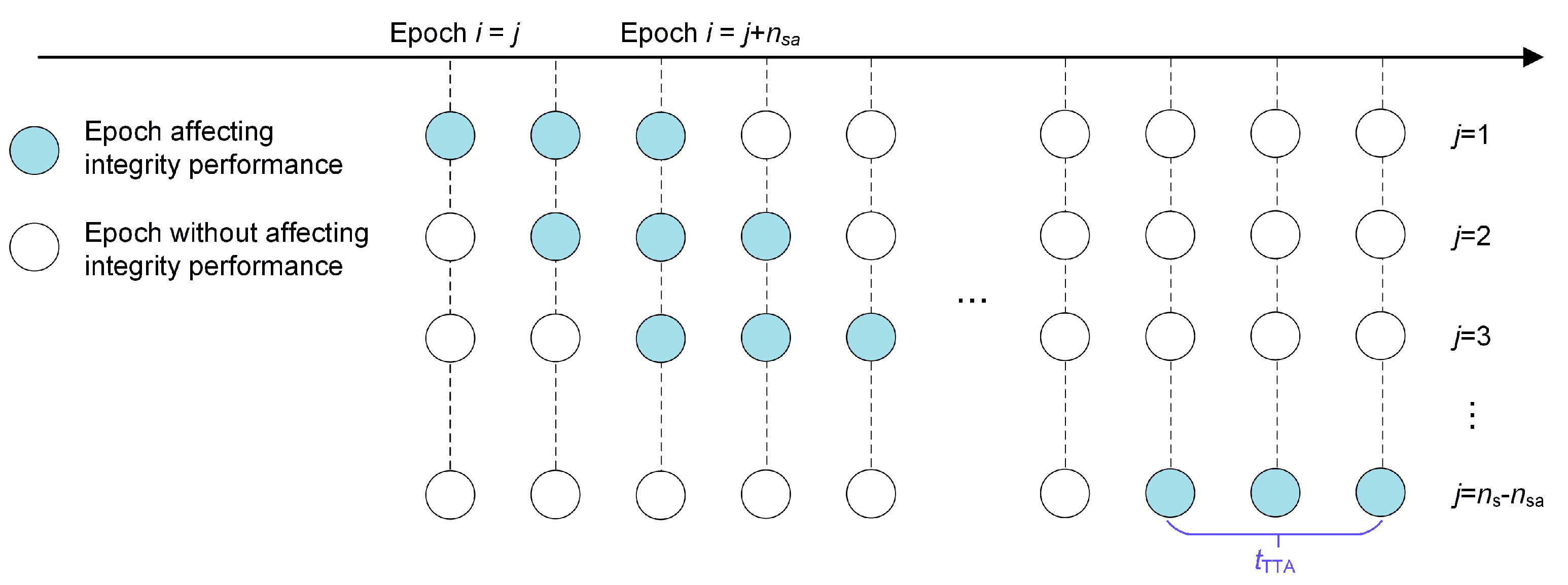
With the definition of HMI, this section applies it to evaluate the integrity risk over the exposure interval. Figure 2 illustrates the epochs that are essential to consider for the integrity risk evaluation under a specific fault mode. Figure 2 indicates that an HMI event will have an impact on navigation safety only when its duration exceeds the time length of tTTA. Additionally, HMI events can potentially occur at any point within the exposure interval. Therefore, a rigorous integrity risk evaluation requires the incorporation of geometry information from all epochs across the exposure interval.
The integrity risk within the exposure interval can be derived from (2) by summing up the probabilities of across all fault modes and epochs. For clarity, we will only present the expression for the integrity risk in a single tTTA under a specific fault event k,
where . Due to the positioning error being highly time-correlated within the allowable time-to-alert, we introduce the PIE to accurately deal with the impact of time-correlation and satellite geometry variation on the integrity risk evaluation simultaneously. The probabilistic PIE is a method used to calculate the probability of unions of events [12]. Based on the PIE, the probability of the occurring under fault mode hypothesis Hk can be described as follows:
where the intersection of is descried as to simplify notations. Given the threshold , the probability of the can be expressed as follows,
where the sequence of random vectors composed of the positioning errors, i.e., . Equation (9) involves a multidimensional-integration calculation. In this paper, the MATLAB function mvncdf was used to implement the integral calculation. Moreover, the normalized positioning errors covariance matrix of adjacent epochs can be expressed as
where β is the reciprocal time constant of the first-order Gaussian Markov process. Δt is a time interval between adjacent two x’s. The sample rate of the receiver ts is typically 0.2–0.5 s based on 2–5 Hz sampling frequencies. For the purposes of this article, a lower sampling interval of 2 s is employed to ease computation times for the MC simulation described below. This is a conservative parameter setting from the perspective of integrity risk evaluation, which was proved by [21]. Furthermore, the numerical examples in Section 4 are calculated for several values of the reciprocal time constant β, ranging from 10 to 1000, to represent different levels of correlation strength.
Here, the integrity risk over the exposure interval can be determined by substituting (7) into (2). In the current ARAIM algorithm, the evaluation of integrity risk often disregards the influence of allowable tTTA, which results in a conservative evaluation result. In contrast, we chose to accurately calculate the integrity risk within the allowable tTTA. The impact of geometry variation on the ARAIM’s integrity performance can be evaluated.
The integrity risk evaluation method has been described in the above related sections, and the detailed integrity risk evaluation process can be described below:
Step 1. Run geometry simulation to obtain the satellite geometry information within the exposure interval in specified time.
Step 2. Collect all the geometry matrix Hi in the exposure interval and calculate based on (4). The will be employed later to reflect satellite geometry variation.
Step 3. Describe the time-correlation effect of the HMI events in the allowable tTTA and determine the normalized positioning errors covariance matrix of adjacent epochs based on (10).
Step 4. Given the and determined by step 2 and step 3, calculate the integrity risk based on (7) and (8) across all fault modes and epochs.
Step 5. Substitute (7) on (2), and calculate the actual integrity risk in the entire exposure interval.
In order to rigorously examine the integrity performance of the ARAIM, an integrity risk evaluation method is proposed to account for the satellite geometry variation in the exposure interval. The integrity performance of the ARAIM under different exposure interval times will be tested later.
4. Experiment and Analysis
In order to examine the integrity performance of the ARAIM, we conducted PHMI simulations based on the proposed method. First, we analyzed the bounding tightness of the evaluated PHMI,actual to the reference PHMI,ref. Second, a worldwide ARAIM integrity performance analysis based on a combination of GPS and Galileo constellation was carried out using the proposed method. The baseline simulation conditions, which are specified in some earlier works [13,26,27,28], were applied to the analysis, and those conditions are also shown in Table 1. Based on the open-source software MAAST for ARAIM Version 0.4 of Stanford University (https://gps.stanford.edu/resources/software-tools/maast, accessed on 4 June 2023), the GPS and Galileo dual constellations were used for the global simulation experiment. The GPS and Galileo almanac files contained in MAAST were used. The global simulation parameters came from ARAIM Technical Subgroup [1] and are listed in Table 1.
4.1. Tightness Analysis of Integrity Risk Evaluate Results
In this section, we will analyze the bounding tightness of the proposed method for the reference. Bounding tightness is a critical characteristic for assessing the performance of an integrity risk-evaluation method. Firstly, it necessitates that the evaluation results are more conservative than the reference results. Secondly, the closer the evaluation results are to the reference, the better the bounding tightness. The purpose of this analysis is to prove the proposed method’s effectiveness in verifying the performance of ARAIM. If the evaluation results of the proposed method are consistently lower than the reference, the subsequent performance verification will be too optimistic. Conversely, if they are significantly higher than the reference, it would lead to an excessively conservative performance verification. We chose the MAAST for ARAIM Version 0.4 software (from Stanford University in Stanford, CA, USA) as the simulation platform, and took the Beijing site as an example to show the relationship between the evaluated results obtained from the proposed method and the reference. It should be noted that the reference was obtained by MC simulation based on (1). Satellite observation error in MC simulation follows the first-order Gaussian Markov model, and the specific model setting can be referred to in [15]. Unfortunately, a full numerical evaluation based on MC simulation would be too computationally taxing for an PHMI,REQ of 10−7 over exposure interval. For instance, considering the RNP 0.1 phase, this would require the simulation of a Gaussian Markov process for at least 107 h, which is more than a thousand years. This limitation is the reason that MC simulation is not directly employed to analyze the performance of the ARAIM. In the tightness analysis simulations, we implemented two settings to mitigate the time-consuming simulations: Firstly, we only tested the Galileo constellation fault situation, as it is the most crucial fault mode impacting the integrity performance of the ARAIM. Secondly, we artificially set VAL to 15 m and HAL to 20 m. This was performed to avoid a considerable number of invalid MC simulations caused by extremely low integrity risk. Our tests mainly include two situations: LPV-200 for V-ARAIM and RNP 0.1 flight phase for H-ARAIM. The total simulation duration for both situations was 10 days, including the LPV-200 approach for 5760 times and the RNP 0.1 phase simulation for 960 times. It should be noted that in the RNP 0.1 phase simulation, a sliding window of 3600 s with the step of 4 s was utilized to increase the test samples. The number of MC simulations was 105, which is significantly higher than the required number of MC simulations converted from PHMI,REQ/10−4. It should be noted that 10−4 represents the prior probability of the Galileo constellation fault, and the calculation is based on the Rconst and MFD. We have collected four types of integrity risk results: the integrity risk reference derived from MC simulation, the minimum and maximum integrity risks within the exposure interval obtained from NES-based ARAIM, and the actual integrity risk obtained from the proposed method.
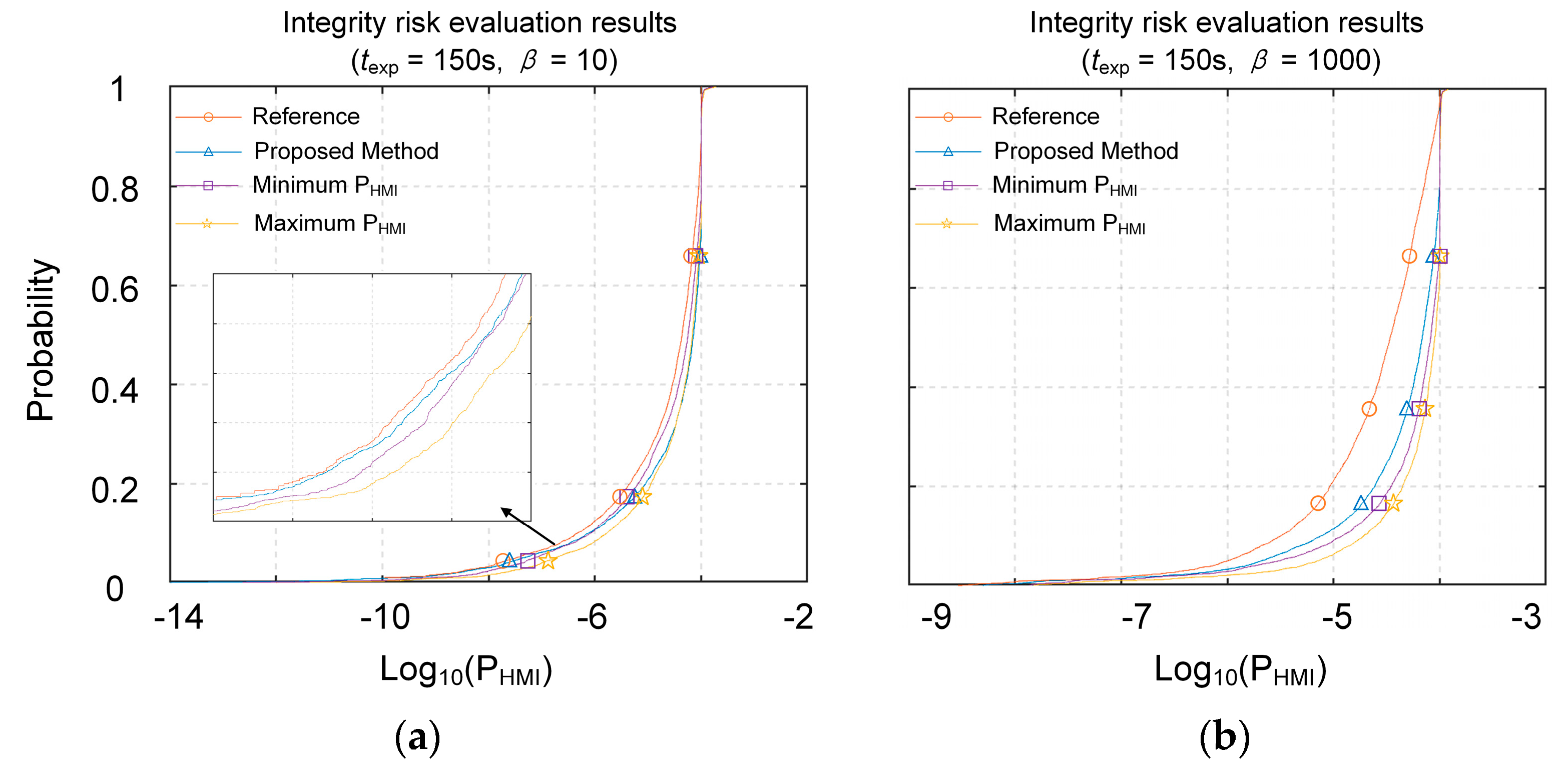
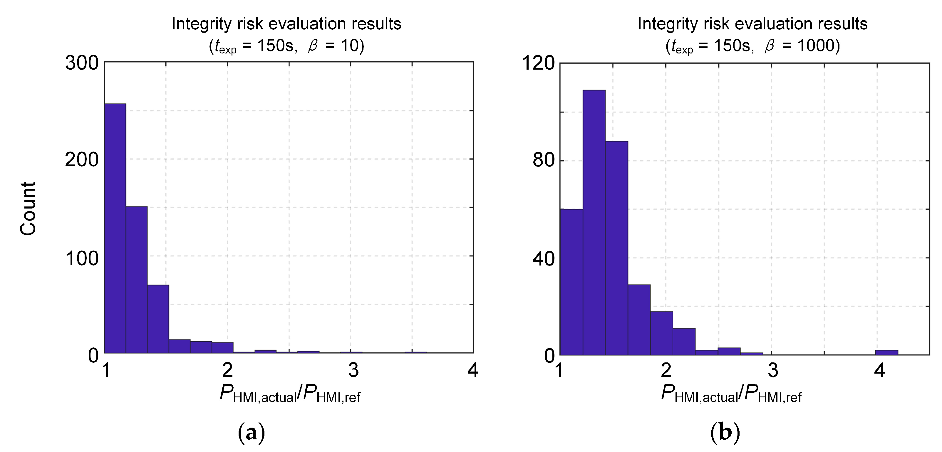
Figure 3 and Figure 4 illustrate the evaluation tightness of the proposed method. β = 10 and β = 1000 were utilized to represent the cases with weak and strong time correlations of positioning errors, respectively. In cases of the low error correlation, as indicated in Figure 3, the empirical cumulative distribution functions (ECDFs) based on the actual integrity risk and reference were very close. This means that the proposed method effectively reflects the integrity risk reference. However, in cases of strong error correlation, the difference between the actual integrity risk results and reference increased. This is attributed to our assumption that is independent of time during the integrity risk evaluation, which leads to conservative evaluation results as the positioning error correlation increases. The more conservative the actual integrity risk, the higher the likelihood of a false decision occurring in the subsequent performance analysis is. The false decision implies that the integrity risk reference is below PHMI,REQ, but according to the proposed method, we conclude that ARAIM is not available. In order to analyze whether the evaluation results are too conservative, we further analyzed the bounding tightness of the actual integrity risk to the reference. We chose the ratio between the actual integrity risk and the reference as the tightness index. It should be noted that we only considered the reference results below 10−7/approach for analysis, as results greater than this threshold would not lead to a false decision. As shown in Figure 4, the tightness index of the proposed method is mostly less than 2. This implies that a false decision occurs only when the reference integrity risk is extremely close to the predefined PHMI,REQ, for instance, falling within the range of 5 × 10⁻⁸/approach to 1 × 10⁻⁷/approach. Furthermore, according to the analysis by [20], due to the high sensitivity of integrity risk to geometry variation, it usually either falls significantly below the PHMI,REQ or notably exceeds the requirement, and rarely falls near the PHMI,REQ. The bounding tightness analysis implies that the proposed method has the ability to verify the ARAIM integrity performance in an LPV-200 approach.
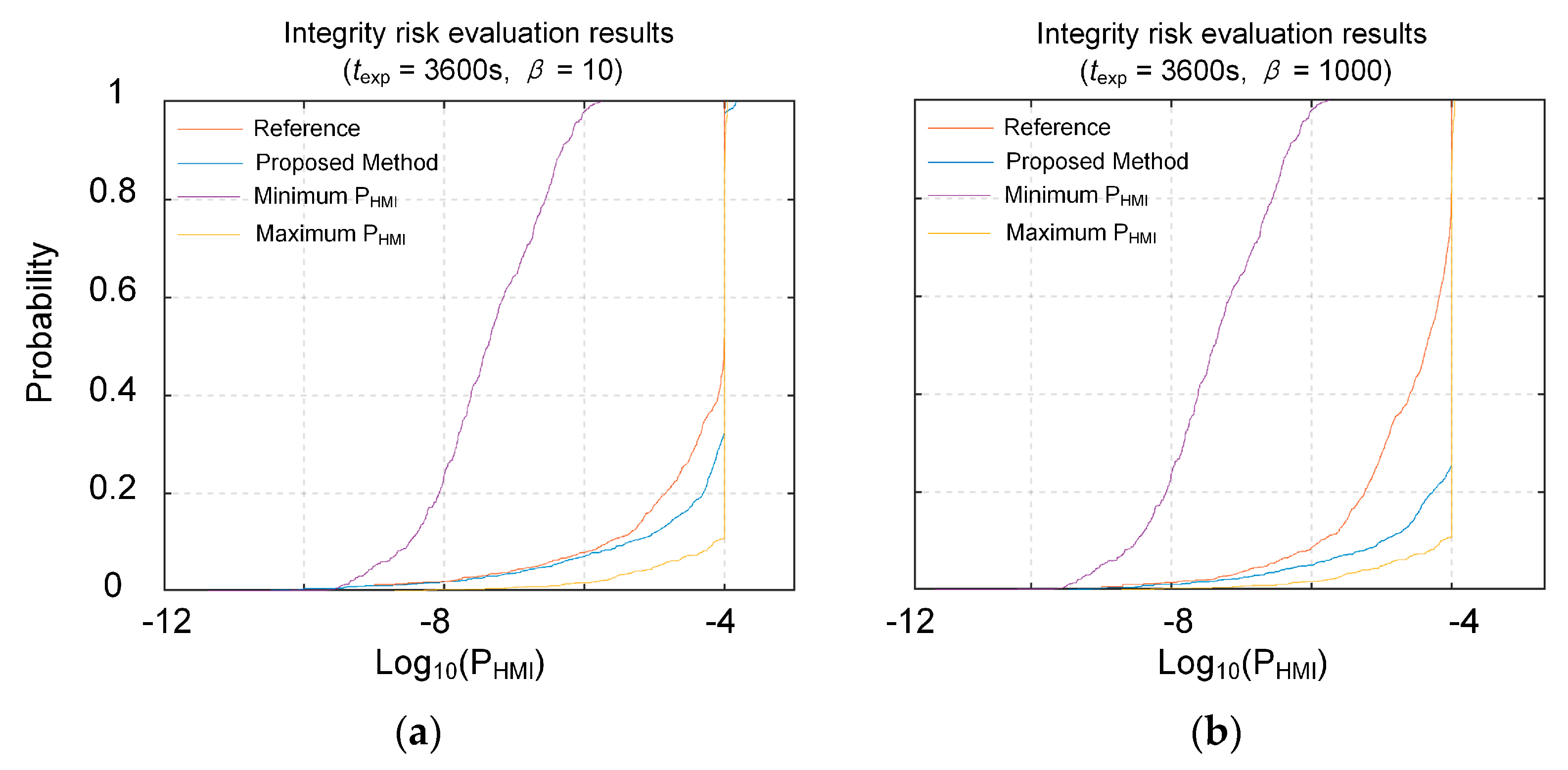
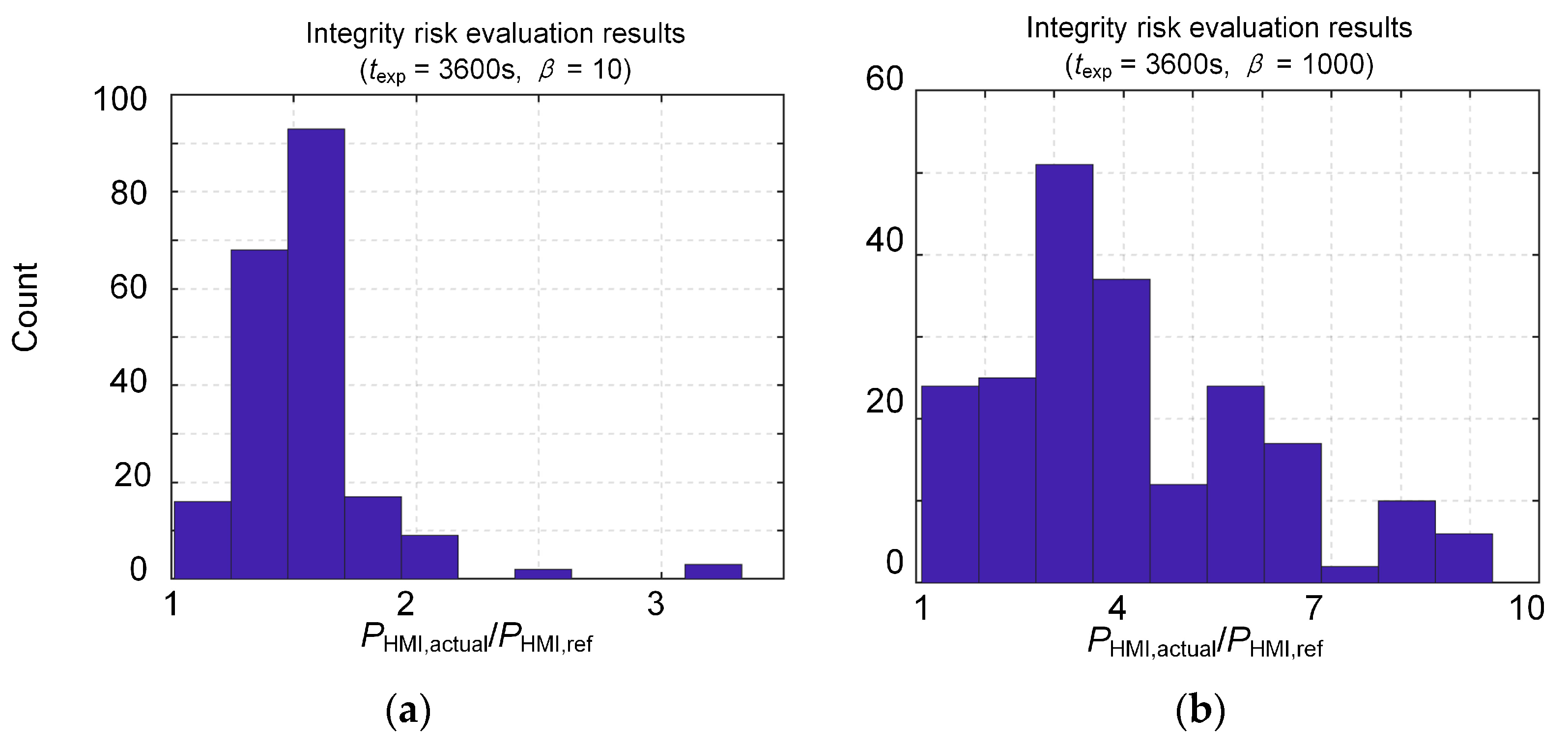
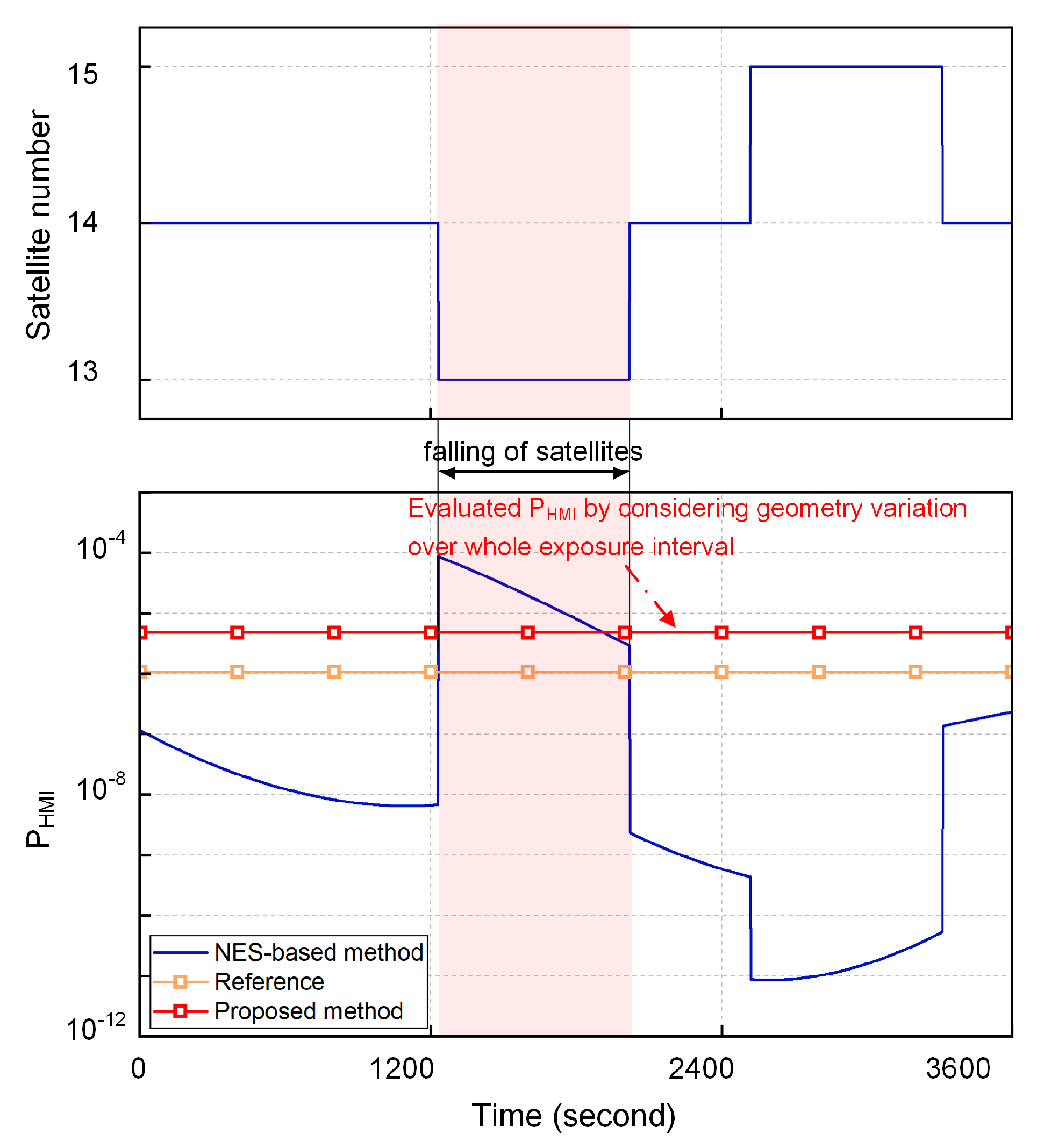
Figure 5 and Figure 6 illustrate the integrity evaluation results under the RNP 0.1 flight phase. Compared with LPV-200, the tightness index of the proposed method is noticeably increased under RNP 0.1, especially when β = 1000. In this scenario, the bounding tightness of the proposed method significantly deteriorates, and the maximum tightness index reaches nearly 10. This indicates that the evaluation error of the proposed method increases with the lengthening of the exposure interval. Fortunately, the AL during the RNP 0.1 phase is relatively loose, implying that the integrity risk is significantly lower than the PHMI,REQ. The high tightness index of the proposed method will not cause many false decisions. This conclusion will be further proved in the subsequent global simulation analysis. Moreover, a notable observation in Figure 5 is that the maximum and minimum evaluation results obtained from the NES-based integrity risk evaluation method vary significantly within the exposure interval, and the ECDF generated by the minimum evaluation results does not effectively bound the reference. This occurs primarily due to the longer duration of the exposure interval in RNP 0.1, leading to more obvious satellite geometry variation during this interval. By comparison, the proposed method can achieve a rigorous bounding for the reference risk value. This is because our method rigorously considers all epoch information when evaluating the integrity risk. Overly optimistic evaluation results pose a significant threat to the integrity of navigation services. This underscores the notable advantages of the proposed method over traditional approaches in ensuring the reliability of navigation services. In Figure 7, an illustrative example of an exposure interval at the Beijing station is selected, demonstrating fluctuations in the number of satellites. The straight line depicted in Figure 7 represents the evaluated risk value by considering geometry variation over the whole exposure interval, so it does not change with time. Since the NES-based ARAIM evaluation result only relies on the single-epoch information throughout the exposure interval, most of the integrity risk evaluation results in Figure 7 are obviously underestimated. On the contrary, the proposed method can effectively bind the reference. Based on the above analysis, we can conclude that the traditional integrity risk evaluation method may be overly optimistic during the RNP 0.1 phase. Therefore, it is necessary to quantify the impact of satellite geometry variation on the ARAIM performance. Subsequently, we utilized the proposed method to validate the worldwide integrity performance of the ARAIM.
4.2. Evaluation of PHMI for Solution Separation ARAIM
To analyze the impact of satellite geometry variations on the integrity performance of the ARAIM, three simulations were conducted under different situations of satellite geometry variation: the first simulation situation is the LPV-200 in a nominal situation, with an exposure interval time of 150 s. The second is the LPV-200 under a one-satellite outage situation. The third situation is RNP 0.1 phase, with an exposure interval time of 3600 s. For the one-satellite outage situation, a satellite was randomly selected as an outage within the exposure interval, and this outage lasted for 30 s. These settings are commonly employed to simulate ionospheric scintillation conditions [18]. The underlying vital assumptions and parameters specified in [13] are used to perform the simulations. The dual-frequency 24 GPS/Galileo nominal constellation with formal parameters was used, and the results were assessed for V-ARAIM (LPV-200) and H-ARAIM (RNP 0.1) operation, respectively. The global simulation was based on a 10° × 10° user grid, for 24 h with a sampling interval of 10 min, which generated 144 samples per user grid. The cut-off elevation angle was set as 5° to balance the observation accuracy and visible satellite. The availability of a grid point can be determined by calculating the ratio of epochs where the evaluated integrity risk is less than the required PHMI,REQ to the total number of epochs during the simulation duration. The global availability coverage was used as the metric to reflect the global integrity performance, which was calculated as the ratio between the number of user grids with the integrity risk smaller than the required PHMI,REQ and the total number of grids. In addition, we chose the minimum value to represent the integrity risk throughout the exposure interval evaluated by the NES-based ARAIM.
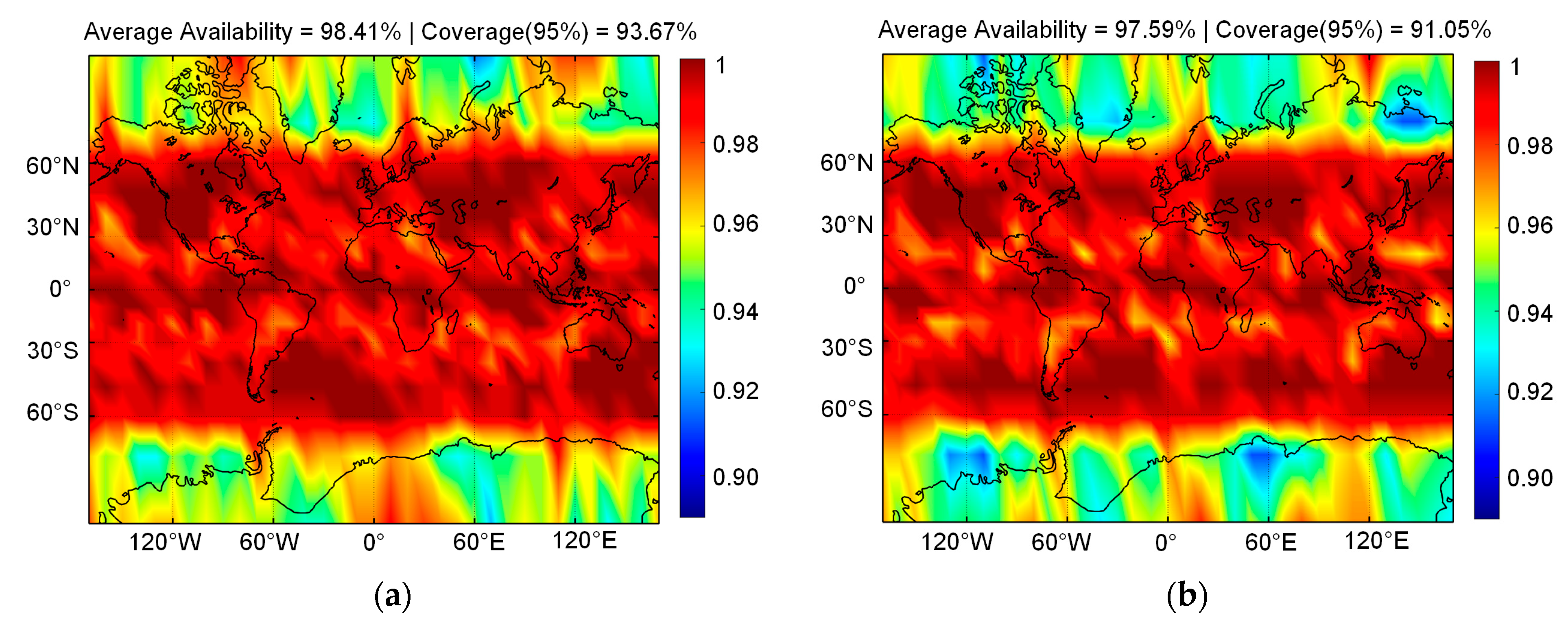
Figure 8 shows the global availability of V-ARAIM in the nominal LPV-200 situation with β = 100. According to Figure 8, the availability of the ARAIM under the traditional method is very close to the actual availability. This indicates that the impact of satellite geometry variation on the integrity performance of the ARAIM is extremely low at a short exposure interval. Furthermore, we summarize the global availability results of the ARAIM under different time correlation strengths of positioning error in Table 2. It can be seen that under weak correlation (β = 10), the ARAIM’s average availability loss is the lowest. When β increases to 100, the average availability loss increases from 0.24% to 0.82%. This is because the weak geometry could continue to affect multiple epochs as the correlation strength of positioning error increases. However, this does not imply that the average availability of the ARAIM will consistently decrease with the increase in β. When β is equal to 1000, the average availability increases by 0.12% compared to β = 100. This is because when the correlation is strong, the integrity performance of the ARAIM mainly depends on the first epoch in the exposure interval, and there may be only one opportunity for an HMI event to occur in this interval. According to the above analysis, under a short exposure interval, the loss in availability caused by the geometry constant assumption is low and does not change significantly with the β value. As a result, traditional methods do not result in overly optimistic integrity risk evaluation results under a short exposure interval.
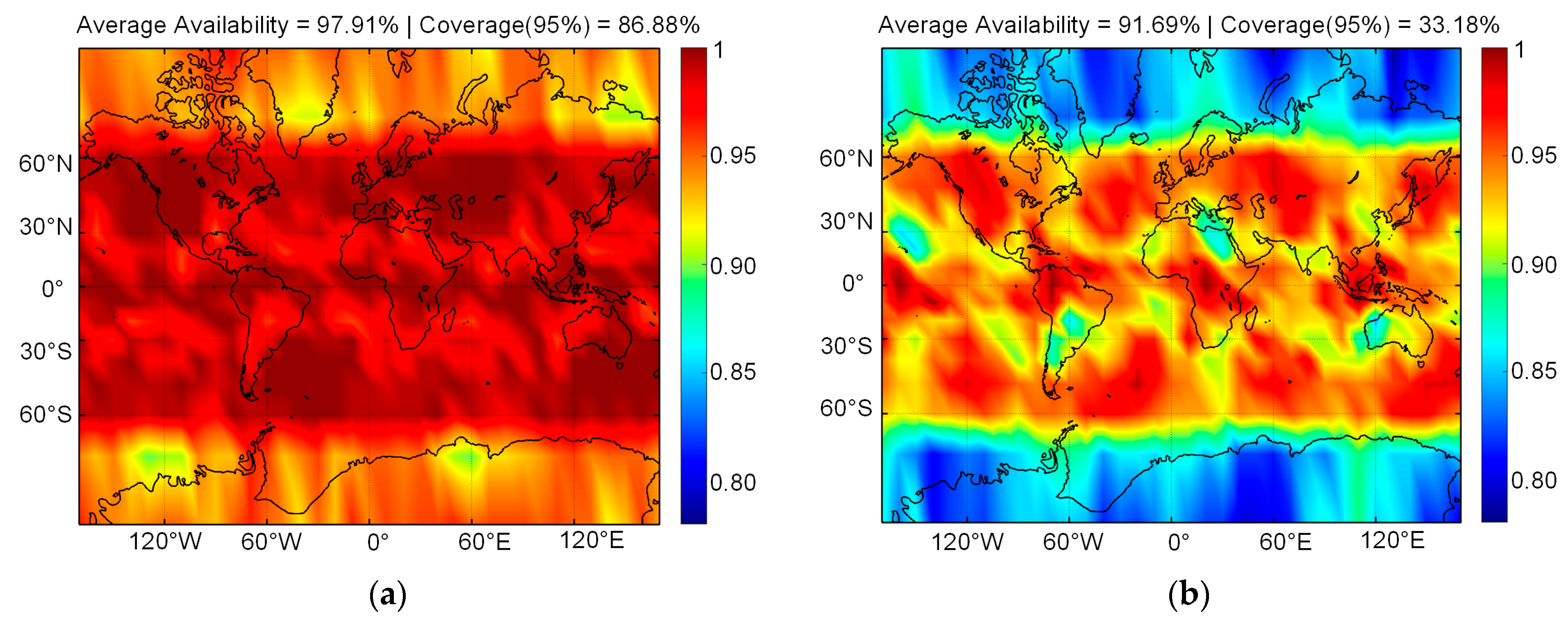
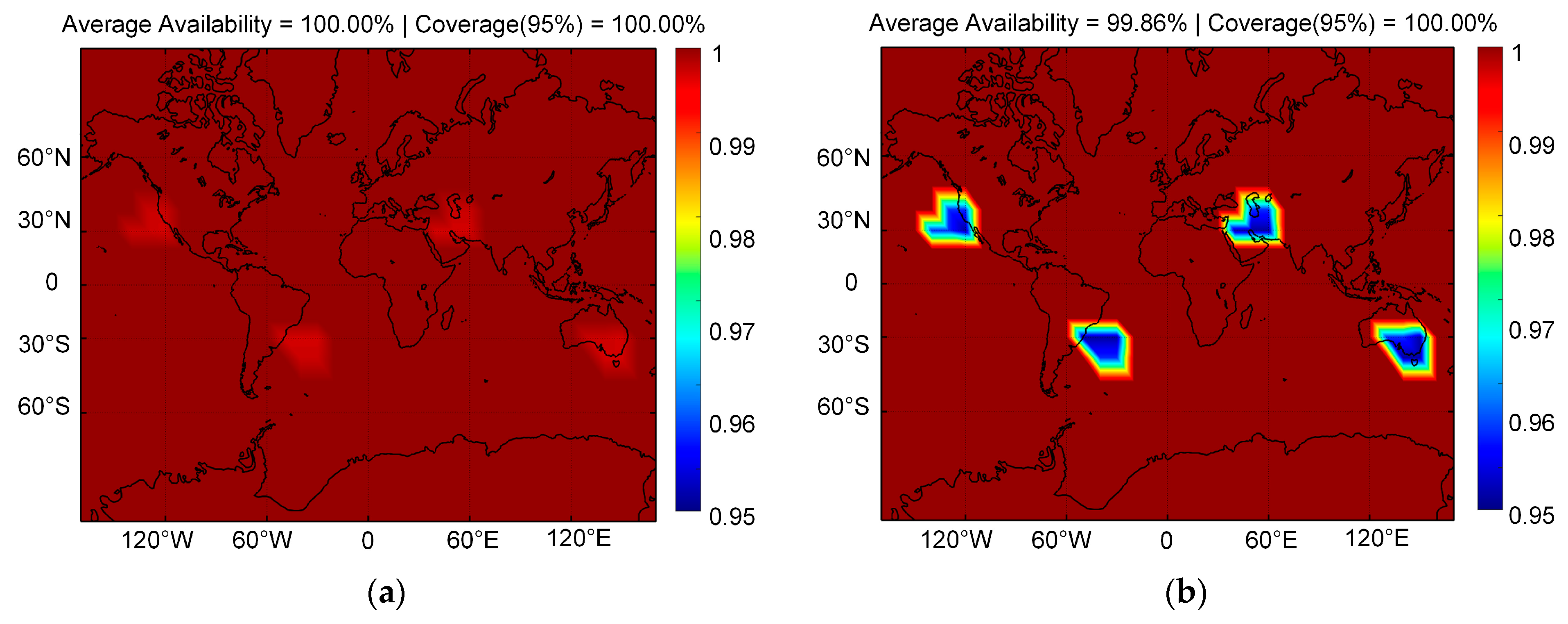
Figure 9 shows the global availability of V-ARAIM in the LPV-200 under a one-satellite outage situation. It can be seen that the absence of one satellite during the interval significantly impacts the integrity performance of navigation applications. Compared to situation 1, the region where the actual ARAIM achieves a 95% availability is reduced by 57.87%. In contrast, the ARAIM determined by the traditional method is only reduced by 6.79%. This indicates that the traditional method is overly optimistic in evaluating the integrity risk based only on the current epoch. In particular, when β equals 100, the ARAIM’s availability decreases more obviously. According to the global simulation results, the average availability loss significantly increased to 6.94%, and the coverage meeting 95% availability was reduced by 53.70%. As far as we know, ARAIM currently utilizes carrier smoothing code (CSC) to mitigate high-frequency code noise, and the time constant of the CSC is also set at 100. Therefore, satellite geometry variations must be taken into account for integrity risk evaluation, particularly in situations involving aircraft banking and ionospheric scintillation. One potential approach to rigorously evaluate the integrity risk is to utilize multiple-epoch information through batch processing or filtering methods [18]. This will be discussed further in our future work. Finally, we analyzed the availability of H-ARAIM in the RNP 0.1 phase. According to Figure 10, it can be seen that the availability loss of traditional ARAIM during this phase is small. This is because the HAL during the RNP 0.1 phase is very loose, resulting in significantly lower integrity risks than the PHMI,REQ. According to Table 2, the maximum loss of average availability based on NES-based ARAIM evaluation is only 0.17%.
Based on the above analysis, this study demonstrates the impact of satellite geometry variation on the integrity performance of NES-based ARAIM. Firstly, the previously geometry constant assumption for the ARAIM integrity risk evaluation does not appear to be overly optimistic under nominal conditions for LPV-200 and RNP 0.1 phases. However, when the navigation applications encounter situations involving aircraft banking and ionospheric scintillation, the traditional method of integrity risk evaluation could become overly optimistic.
5. Conclusions
We conducted a preliminary assessment of NES-based ARAIM integrity performance by presenting a methodology to calculate the actual integrity risk based on a geometry-sensitive risk-evaluation model. According to the simulation analysis, compared with the reference risk value, the results evaluated by traditional NES-based ARAIM methods are usually proved to be optimistic. In contrast, the proposed method can realize rigorous bounding for the reference risk value by considering all epoch information within the exposure interval during the evaluation of integrity risk. Using the proposed method and baseline conditions, we rigorously analyzed the impact of satellite geometry variation on the ARAIM integrity performance over the exposure interval. Several key conclusions are summarized as follows.
First, in the nominal LPV-200 with 150 s exposure interval time and the nominal RNP 0.1 with 3600 s, the traditional NES-based ARAIM does not produce overly optimistic integrity risk-evaluation results. According to the global simulation results, the maximum average availability loss of traditional method is only 0.82% after considering the impact of satellite geometry variation.
Second, in the situation of a single-satellite outage during LPV-200 approach, the traditional method is overly optimistic in evaluating the integrity risk based on the geometry constant assumption. According to the global simulation results, the average availability loss has significantly increased to 6.94%, and the coverage meeting 95% availability has reduced by 53.70%. This implies that ensuring the rigor of integrity risk evaluation in the case of aircraft banking and ionospheric scintillation is challenging for the NES-based method.
Finally, a potential real-time integrity risk evaluation approach is briefly introduced, which involves utilizing multiple-epoch information through batch processing or filtering methods. In future research, we will focus on applying these methods to enhance the current ARAIM algorithm.
Author Contributions
Conceptualization, R.L., L.L., and Z.N.; methodology, R.L. and L.L.; validation, Z.N., Y.D., and X.X.; formal analysis, Y.D. and X.X.; investigation, L.L. and Z.L.; resources, R.L. and L.L.; writing—original draft preparation, R.L; writing—review and editing, R.L. and L.L.; visualization, R.L., Z.N., and Z.L.; supervision, Z.N. and Z.L.; project administration, L.L.; funding acquisition, L.L. All authors have read and agreed to the published version of the manuscript.
Funding
National Key Research and Development Program (No. 2021YFB3901300), the National Natural Science Foundation of China (Nos. 62373117 and 62003109), the Fundamental Research Funds for Central Universities (Nos. 3072019CF0401, 3072020CFT0403).
Data Availability Statement
Data are contained within the article.
Conflicts of Interest
The authors declare no conflicts of interest.
References
- WG-C Advanced RAIM Technical Subgroup (TSG). Advanced RAIM Technical Subgroup Reference Airborne Algorithm Description Document v4.1. 2022. Available online: https://www.ion.org/publications/abstract.cfm?articleID=18254 (accessed on 4 June 2023).
- Lee, Y.; Bian, B.; Odeh, A.; She, J. Sensitivity of advanced RAIM performance to mischaracterizations in integrity support message values. J. Navig. 2021, 68, 541–558. [Google Scholar] [CrossRef]
- Li, L.; Li, Z.; Yuan, H.; Wang, L.; Hou, Y. Integrity monitoring-based ratio test for GNSS integer ambiguity validation. GPS Solut. 2016, 20, 573–585. [Google Scholar] [CrossRef]
- Zhao, Y.; Cheng, C.; Li, L.; Wang, R.; Liu, Y.; Li, Z.; Zhao, L. BDS signal-in-space anomaly probability analysis over the last 6 years. GPS Solut. 2021, 25, 49. [Google Scholar] [CrossRef]
- Ma, X.; He, X.; Yu, K.; Montillet, J.P.; Lu, T.; Yan, L.; Zhao, L. Progress of global ARAIM availability of BDS-2/BDS-3 with TGD and ISB. Adv. Space Res. 2022, 70, 935–946. [Google Scholar] [CrossRef]
- Li, L.; Zhao, L.; Yang, F.; Li, N. A novel ARAIM approach in probability domain for combined GPS and Galileo. In Proceedings of the 28th International Technical Meeting of the Satellite Division of The Institute of Navigation (ION GNSS+ 2015), Tampa, FL, USA, 14–18 September 2015. [Google Scholar]
- Blanch, J.; Walter, T.; Enge, P. RAIM with optimal integrity and continuity allocations under multiple failures. IEEE Trans. Aerosp. Electron. Syst. 2010, 46, 1235–1247. [Google Scholar] [CrossRef]
- Bang, E.; Milner, C.; Macabiau, C. Cross-correlation effect of ARAIM test statistic on false alarm risk. GPS Solut. 2020, 24, 1–14. [Google Scholar] [CrossRef]
- Li, L.; Wang, H.; Jia, C.; Zhao, L.; Zhao, Y. Integrity and continuity allocation for the RAIM with multiple constellations. GPS Solut. 2017, 21, 1503–1513. [Google Scholar] [CrossRef]
- Yang, Y.; Gao, W.; Guo, S.; Mao, Y.; Yang, Y. Introduction to BeiDou-3 navigation satellite system. Navigation 2019, 66, 7–18. [Google Scholar] [CrossRef]
- Joerger, M.; Chan, F.; Pervan, B. Solution separation versus residual-based RAIM. J. Navig. 2014, 61, 273–291. [Google Scholar] [CrossRef]
- Milner, C.; Ochieng, W.Y. Weighted RAIM for APV: The ideal protection level. J. Navig. 2011, 64, 61–73. [Google Scholar] [CrossRef]
- Blanch, J.; Walter, T.; Enge, P.; Lee, Y.; Pervan, B.; Rippl, M.; Spletter, A.; Kropp, V. Baseline advanced RAIM user alogothrim and possible improvements. IEEE Trans. Aerosp Electron. Syst. 2015, 51, 713–732. [Google Scholar] [CrossRef]
- Zhai, Y.; Zhan, X.; Pervan, B. Bounding Integrity Risk and False Alert Probability Over Exposure Time Intervals. IEEE Trans. Aerosp Electron. Syst. 2019, 56, 1873–1885. [Google Scholar] [CrossRef]
- Milner, C.; Pervan, B.; Blanch, J.; Joerger, M. Evaluating integrity and continuity over time in advanced RAIM. 2020. In Proceedings of the IEEE/ION Position, Location and Navigation Symposium (PLANS), Portland, OR, USA, 20–23 April 2020. [Google Scholar]
- Blanch, J.; Walter, T.; Milner, C.; Joerger, M.; Pervan, B.; Bouvet, D. Baseline advanced RAIM user algorithm: Proposed updates. In Proceedings of the 2022 International Technical Meeting of The Institute of Navigation (ION ITM 2022), Long Beach, CA, USA, 25–27 January 2022. [Google Scholar]
- Du, J.; Wang, Z.; Fang, K.; Zhu, Y.; Dan, Z.; Wang, H.; Li, X. ARAIM integrity risk allocation over time. In Proceedings of the 35th International Technical Meeting of the Satellite Division of The Institute of Navigation (ION GNSS+ 2022), Denver, CO, USA, 19–23 September 2022. [Google Scholar]
- Blanch, J.; Chen, Y.; Phelts, R.; Walter, T.; Enge, P. Mitigation of short duration satellite outages for Advanced RAIM and other integrity systems based on GNSS. In Proceedings of the 29th International Technical Meeting of the Satellite Division of the Institute of Navigation (ION GNSS+ 2016), Portland, OR, USA, 12–16 September 2016. [Google Scholar]
- Nikiforov, I. From pseudorange overbounding to integrity risk overbounding. Navigation 2019, 66, 417–439. [Google Scholar] [CrossRef]
- Lee, Y.; She, J.; Odeh, A.; Bian, B. Horizontal advanced RAIM performance sensitivity to mischaracterizations in integrity support message values. In Proceedings of the 32nd International Technical Meeting of the Satellite Division of the Institute of Navigation (ION GNSS+ 2019), Miami, FL, USA, 16–20 September 2019. [Google Scholar]
- Bang, E.; and Milner, C. Integrity risk under temporal correlation for horizontal ARAIM. IEEE Trans. Aerosp Electron. Syst. 2021, 57, 3974–3987. [Google Scholar] [CrossRef]
- Joerger, M.; Pervan, B. Multi-constellation ARAIM exploiting satellite motion. Navigation 2020, 67, 235–253. [Google Scholar] [CrossRef]
- Zhai, Y. Ensuring Navigation Integrity and Continuity Using Multi-Constellation GNSS. Ph.D. Thesis, Department of Mechanical, Materials and Aerospace Engineering, Illinois Institute of Technology, Chicago, IL, USA, 2018. [Google Scholar]
- Joerger, M.; Stevanovic, S.; Langel, S.; Pervan, B. Integrity risk minimisation in RAIM part 1: Optimal detector design. J. Navig. 2016, 69, 449–467. [Google Scholar] [CrossRef]
- Chan, F.; Joerger, M.; Khanafseh, S.; Pervan, B. Bayesian fault-tolerant position estimator and integrity risk bound for GNSS navigation. J. Navig. 2014, 67, 753–775. [Google Scholar] [CrossRef]
- Cassel, R. Real-Time ARAIM Using GPS, GLONASS, and GALILEO. Master’s Thesis, Department of Mechanical, Materials and Aerospace Engineering, Illinois Institute of Technology, Chicago, IL, USA, 2017. [Google Scholar]
- Wang, L.; Luo, S.; Tu, R.; Fan, L.; Zhang, Y. ARAIM with BDS in the Asia-Pacific region. Adv. Space Res. 2018, 62, 707–720. [Google Scholar] [CrossRef]
- El-Mowafy, A.; Yang, C. Limited sensitivity analysis of ARAIM availability for LPV-200 over Australia using real data. Adv. Space Res. 2016, 57, 659–670. [Google Scholar] [CrossRef]
Figure 1.
Epochs over the exposure interval.

Figure 2.
A conceptual illustration of the integrity risk evaluation within exposure interval.

Figure 3.
Integrity risk evaluation results of different methods under LPV-200 situation. The subfigure (a,b) indicates that β is 10 and 1000, respectively.
Figure 3.
Integrity risk evaluation results of different methods under LPV-200 situation. The subfigure (a,b) indicates that β is 10 and 1000, respectively.

Figure 4.
Histogram of the tightness index of the proposed method under LPV-200 situation. The subfigure (a,b) indicates that β is 10 and 1000, respectively.
Figure 4.
Histogram of the tightness index of the proposed method under LPV-200 situation. The subfigure (a,b) indicates that β is 10 and 1000, respectively.

Figure 5.
Integrity risk evaluation result of different methods under RNP-0.1 situation. The subfigure (a,b) indicates that β is 10 and 1000, respectively.
Figure 5.
Integrity risk evaluation result of different methods under RNP-0.1 situation. The subfigure (a,b) indicates that β is 10 and 1000, respectively.

Figure 6.
Histogram of the tightness index of the proposed method under RNP-0.1 situation. The subfigure (a,b) indicates that β is 10 and 1000, respectively.
Figure 6.
Histogram of the tightness index of the proposed method under RNP-0.1 situation. The subfigure (a,b) indicates that β is 10 and 1000, respectively.

Figure 7.
Changes in satellite number and integrity risk in 1 h exposure interval. Pink squares indicate areas where the NES-based method is higher than the reference value.
Figure 7.
Changes in satellite number and integrity risk in 1 h exposure interval. Pink squares indicate areas where the NES-based method is higher than the reference value.

Figure 8.
Availability map of the ARAIM under the nominal situation. The subfigure (a,b) represents the availability of ARAIM based on the traditional method and the proposed method, respectively.
Figure 8.
Availability map of the ARAIM under the nominal situation. The subfigure (a,b) represents the availability of ARAIM based on the traditional method and the proposed method, respectively.

Figure 9.
Availability map of the ARAIM with one-satellite outages. The subfigure (a,b) represents the availability of ARAIM based on the traditional method and the proposed method, respectively.
Figure 9.
Availability map of the ARAIM with one-satellite outages. The subfigure (a,b) represents the availability of ARAIM based on the traditional method and the proposed method, respectively.

Figure 10.
Availability map of the ARAIM under RNP 0.1 nominal situation. The subfigure (a,b) represents the availability of ARAIM based on the traditional method and the proposed method, respectively.
Figure 10.
Availability map of the ARAIM under RNP 0.1 nominal situation. The subfigure (a,b) represents the availability of ARAIM based on the traditional method and the proposed method, respectively.


Table 1.
Simulation parameters setting [1].
Table 1.
Simulation parameters setting [1].
| Parameters | Value |
|---|---|
| Satellite clock and orbits correction error σURA (integrity) | V-ARAIM: 1.5 [m] H-ARAIM: 2.4 [m] |
| Satellite clock and orbits correction error σURE (accuracy and continuity) | (2/3) σURA [m] |
| PHMI,REQ | V-ARAIM: 9.8 × 10⁻⁸/150 s H-ARAIM: 1.0 × 10⁻⁷/h |
| PFA,REQ | V-ARAIM: 3.9 × 10⁻⁶/150 sH-ARAIM: 5.0 × 10⁻⁷/h |
| Rsat | 10−5/h for both GPS and Galileo |
| Rconst | 10−8/h (GPS); 1 × 10⁻⁴/h (Galileo) |
| MFD (mean fault duration) | 1 h for both GPS and Galileo |
| NES | texp/ts for both integrity and continuity |
| texp | 150 [s] (LPV-200); 3600 [s] (RNP 0.1) |
| ta | 6 [s] (LPV-200); 10 [s] (RNP 0.1) |
| ts | 2 [s] |
| PNM | 6 × 10⁻⁸ |
| Alarm limit | VAL: 35 [m]; HAL: 185 [m] |
Table 2.
Average availability results and coverage (95%) of the ARAIM.
| Method | β = 10 | β = 100 | β = 1000 | ||||
|---|---|---|---|---|---|---|---|
| Average | Coverage | Average | Coverage | Average | Coverage | ||
| LPV-200 nominal | Traditional | 98.41% | 93.67% | 98.41% | 93.67% | 98.41% | 93.67% |
| Actual | 98.17% | 92.44% | 97.59% | 91.05% | 97.71% | 90.74% | |
| Loss | 0.24% | 1.23% | 0.82% | 2.62% | 0.70% | 2.93% | |
| LPV-200 one-satellite outage | Traditional | 97.91% | 86.88% | 97.91% | 86.88% | 97.91% | 86.88% |
| Actual | 94.51% | 58.02% | 91.69% | 33.18% | 90.97% | 26.39% | |
| Loss | 3.40% | 28.86% | 6.22% | 53.70% | 6.94% | 60.49% | |
| RNP 0.1 | Traditional | 100.00% | 100.00% | 100.00% | 100.00% | 100.00% | 100.00% |
| Actual | 99.86% | 100.00% | 99.86% | 100.00% | 99.83% | 100.00% | |
| Loss | 0.14% | 0.00% | 0.14% | 0.00% | 0.17% | 0.00% | |
Disclaimer/Publisher’s Note: The statements, opinions and data contained in all publications are solely those of the individual author(s) and contributor(s) and not of MDPI and/or the editor(s). MDPI and/or the editor(s) disclaim responsibility for any injury to people or property resulting from any ideas, methods, instructions or products referred to in the content. |
© 2024 by the authors. Licensee MDPI, Basel, Switzerland. This article is an open access article distributed under the terms and conditions of the Creative Commons Attribution (CC BY) license (https://creativecommons.org/licenses/by/4.0/).
Share and Cite
MDPI and ACS Style
Li, R.; Li, L.; Na, Z.; Duan, Y.; Xu, X.; Liu, Z. Impact Analysis of Satellite Geometry Variation on ARAIM Integrity Risk over Exposure Interval. Remote Sens. 2024, 16, 286. https://doi.org/10.3390/rs16020286
AMA Style
Li R, Li L, Na Z, Duan Y, Xu X, Liu Z. Impact Analysis of Satellite Geometry Variation on ARAIM Integrity Risk over Exposure Interval. Remote Sensing. 2024; 16(2):286. https://doi.org/10.3390/rs16020286
Chicago/Turabian StyleLi, Ruijie, Liang Li, Zhibo Na, Yangwang Duan, Xin Xu, and Zelin Liu. 2024. "Impact Analysis of Satellite Geometry Variation on ARAIM Integrity Risk over Exposure Interval" Remote Sensing 16, no. 2: 286. https://doi.org/10.3390/rs16020286
Note that from the first issue of 2016, this journal uses article numbers instead of page numbers. See further details here.