Technical Note

Inversion of Near-Surface Aerosol Equivalent Complex Refractive Index Based on Aethalometer, Micro-Pulse Lidar and Portable Optical Particle Profiler

1
Key Laboratory of Atmospheric Optics, Anhui Institute of Optics and Fine Mechanics, HFIPS, Chinese Academy of Sciences, Hefei 230031, China
2
Science Island Branch of Graduate School, University of Science and Technology of China, Hefei 230026, China
3
Advanced Laser Technology Laboratory of Anhui Province, Hefei 230037, China
4
Nanhu Laser Laboratory, National University of Defense Technology, Changsha 410073, China
*
Author to whom correspondence should be addressed.
Remote Sens. 2024, 16(2), 279; https://doi.org/10.3390/rs16020279
Submission received: 10 October 2023 / Revised: 25 December 2023 / Accepted: 3 January 2024 / Published: 10 January 2024
(This article belongs to the Section Atmospheric Remote Sensing)

Abstract

:
In order to investigate the equivalent complex refractive index of atmospheric aerosols near the Earth’s surface, we conducted measurements in the Hefei region from March to April 2022. These measurements utilized a micro-pulse lidar, an Aethalometer, and a Portable Optical Particle Profiler. These measurements encompassed aerosol particle size distribution as well as standard meteorological parameters including temperature, humidity, atmospheric pressure, and wind speed. Subsequently, this dataset was employed to develop an optimization algorithm for retrieving the equivalent complex refractive indices of near-surface aerosols. The methodology relies on lookup tables containing data for extinction efficiency and absorption efficiency factors. It operates on the premise of aerosol property stability within a defined time frame, utilizing measured extinction and absorption coefficients as simultaneous constraints during this period to inversely derive both the real and imaginary parts of the aerosol complex refractive index. Results from the simulation analysis reveal that the newly optimized retrieval algorithm, which relies on lookup tables, exhibits reduced sensitivity to instrument errors when compared to single-point constraint algorithms. This enhancement results in a more efficient and dependable approach for retrieving the aerosol complex refractive index. Empirical inversion and simulation studies were carried out to determine the aerosol equivalent complex refractive index in the Hefei region, utilizing measured data. This inversion process yielded an average complex refractive index of 1.48-i0.017 for aerosols in the Hefei region throughout the experimental period. Correlation analysis unveiled a positive association between the real part of the aerosol complex refractive index and the single-scattering albedo (SSA), whereas the imaginary part displayed a linear negative correlation with the SSA. The mathematical relationship between the real part and the SSA is y = 0.19 x + 0.62 , and the corresponding relationship between the imaginary part and the SSA is y = 5.3 x + 0.99 . This research offers a novel method for the retrieval of the aerosol equivalent complex refractive index.

Graphical Abstract

1. Introduction

The system of suspended solid particles and droplets dispersed in the atmosphere is called atmospheric aerosols. Atmospheric aerosols may originate from natural sources such as sea waves, desert dust storms, and volcanic activities or from anthropogenic sources such as fossil fuel combustion and biomass burning [1,2,3]. Aerosols in the atmosphere can affect global and regional climate directly by scattering and absorbing solar radiation, and indirectly by modifying cloud properties as condensation nuclei [4,5,6,7]. The most significant uncertainty in estimating the impact of aerosols on climate stems from the uncertainty in determining their geophysical properties, including the complex refractive index of aerosols (ACRI), which in turn determines their radiative properties. These uncertainties may be related to effective emissions, spatial distribution of emission sources, and temporal changes [8].
The ACRI is a crucial parameter driving optical properties and is highly dependent on the chemical composition of the particles. The ACRI comprises both the real and imaginary parts, and these components play a significant role in affecting aerosol scattering and absorption [9,10,11]. The magnitude of radiative forcing is very sensitive to ACRI, and the dependence of radiative forcing on its imaginary part is even more pronounced than that on real part [12]. Therefore, precisely determining the ACRI, especially the imaginary part, is crucial for inferring the optical properties and the impact of aerosols on the climate. However, environmental aerosols are usually complex mixtures of different species, and it is not feasible to calculate the radiative properties of aerosols based on the refractive index of each component within a group of aerosols. Therefore, the effective ACRI of complex mixed particles is often used to represent the entire size distribution [13]. Generally speaking, the aerosol’s equivalent complex refractive index can be obtained using chemical and optical methods. Effective ACRI (chemical method) is often determined from bulk chemical compositions and known values of the refractive index of pure components [14]. In contrast, the effective ACRI (optical method) of a mixture is retrieved from its inherent optical properties and might produce the same (or very similar) optical properties as the intrinsic values under the same particle shapes [8].
In recent years, many studies have been conducted on measuring ACRI. Volume-weighted averaging (VWA), a method for determining the equivalent ACRI of an aerosol-based on chemical properties, was chosen because the ACRI is highly correlated with the chemical properties of the aerosol [14,15,16]. In addition to using chemical methods to determine aerosols’ equivalent refractive index, studies have been conducted to determine the equal complex refractive index using optical techniques applying a spheroidal dust model to derive ACRI from photometer observations of the sun with AERONET (Aerosol Robotic Network) data [17]. With the assumption of spherical particles and chemical homogeneity of aerosol samples, effective ACRI can be retrieved based on simultaneous measurements of size distributions, scattering and absorption coefficients [18,19,20,21,22]. Another study compared ACRI derived from different techniques and found only some reasonable agreement, with the rest of the imaginary part of the spectrum varying widely [23]. Despite the multitude of studies on ACRI, further research is essential to enhance our comprehension, particularly focusing on comprehensive measurements incorporating Mie scattering theory and aerosol characteristics.
This paper presents an optimized algorithm for retrieving the optical equivalent complex refractive index. This method is based on the Mie scattering theory. It uses the joint measurements of near-ground aerosol microphysical and optical properties obtained through a micro-pulse Lidar (MPL), a Portable Optical Particle Profiler (POPS), and an Aethalometer to iteratively invert the equivalent complex refractive index of near-surface aerosols. In Section 2, the instruments and measurement principles employed in the experimental process are detailed. Section 3 provides a detailed overview of the algorithm’s specific approach, sensitivity analysis, and reliability assessment for retrieving the ACRI. Section 4 encompasses the results and discussion.

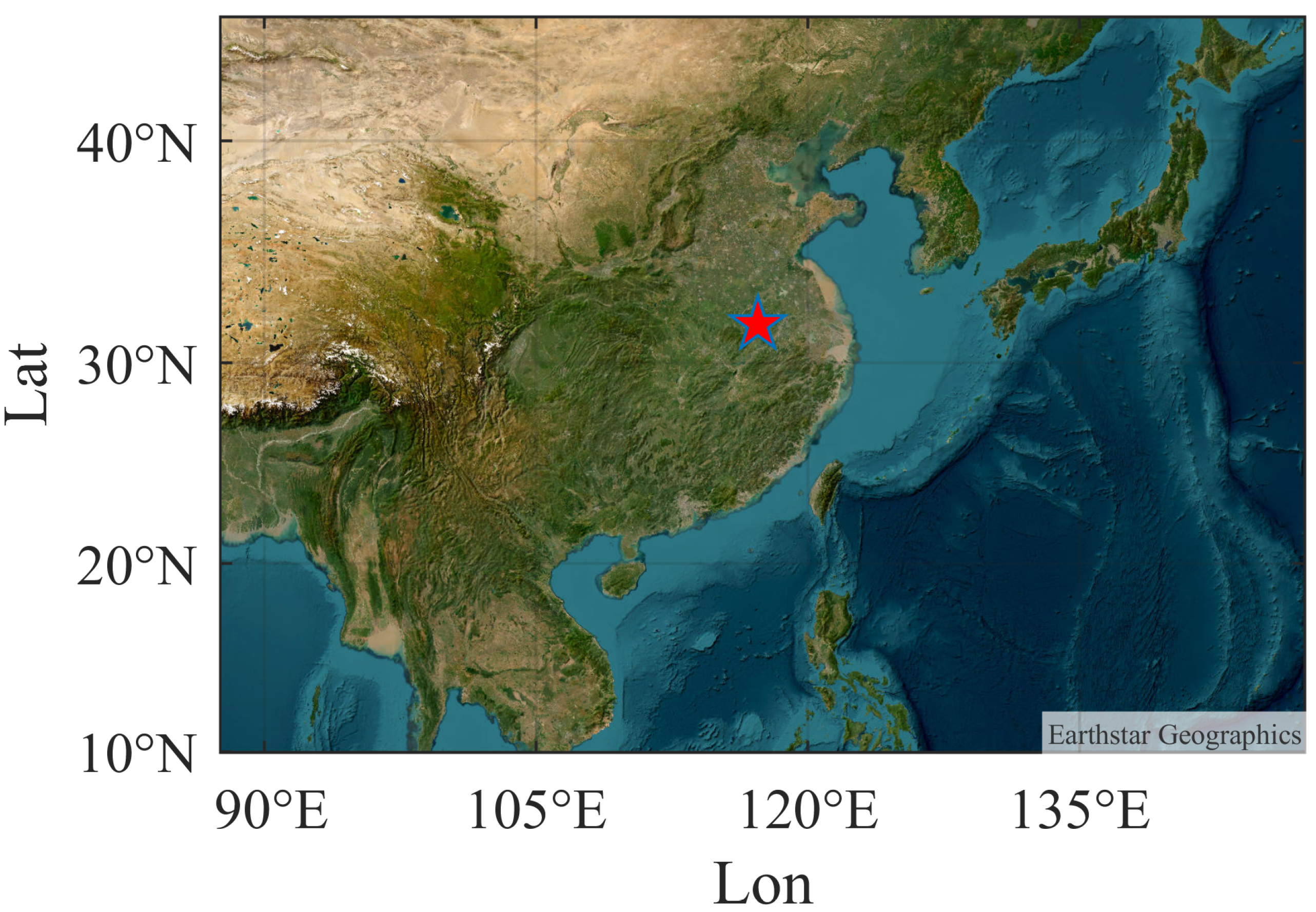
2. Experimental Site and Instrument Introduction

In March and April 2022, a collaborative observational experiment was carried out to investigate aerosol optical and microphysical properties. This experiment utilized a POPS, an MPL, and an Aethalometer and took place at the Atmospheric Optics Center, situated on Hefei Science Island in the western suburbs of Hefei, under the jurisdiction of the Anhui Institute of Optics and Fine Mechanics, Chinese Academy of Sciences (refer to Figure 1). More specifically, the POPS and the Aethalometer were placed about 12 m above the ground for measurements, and the MPL was placed about 9 m above the ground for horizontal measurements. The horizontal distance between the MPL, the Aethalometer, and the POPS was maintained at about 50 m, which ensured that the data were consistent in both the temporal and spatial dimensions.

2.1. Portable Optical Particle Profiler

The Portable Optical Particle Profiler (POPS) [24] manufactured by Handix, serves as an optical instrument employed for the measurement of aerosol particle size distributions. The POPS utilizes an internal pump to intake ambient air and sheath gas into the optical cavity of the instrument. The instrument’s measurement range extends from 130 nm to 3 µm, providing a diameter resolution of about 5%. The POPS typically operates using 16 channels, and the radius of these channels are detailed in Table 1. The instrument is calibrated using standard particles composed of polystyrene microspheres with a refractive index of m = 1.615 + 0.001i.

2.2. Micro-Pulse Lidar

The radar employed in this study is an MPL developed independently by the Anhui Institute of Optics and Fine Mechanics, Chinese Academy of Sciences [25]. The lidar system is primarily composed of three key components: a laser emission unit, a receiving unit, and a signal detection and acquisition unit. It boasts a spatial resolution of 30 m and can detect objects at altitudes of up to 30 km [26]. The laser emission unit is equipped with a 532 nm Nd:YAG laser and an optical beam expander. It incorporates a 5× beam expander, which effectively reduces the laser’s scattering angle from 2.0 mrad to 0.4 mrad. This adjustment enables fine-tuning of the telescope’s receiving field to 0.5 mrad, consequently minimizing daytime sky background radiation and enhancing the system’s detection signal-to-noise ratio. The optical receiving unit primarily captures the backscattered light signals and directs them into distinct detection channels according to their respective wavelengths. This unit comprises a receiving telescope, a pinhole optical stop, and various subsequent optical pathways, among other components.
Presently, inversion algorithms for the extinction coefficient of the MPL primarily encompass the slope method [27], the Klett method [28], and the Fernald method [29]. Since this paper requires the utilization of near-surface aerosol extinction coefficients and seeks to minimize the influence of radar blind spots, horizontal lidar detection is implemented, and the slope method is applied for calculating the horizontal extinction coefficient. Equation (1) illustrates the lidar equation [25]:
P ( r ) = P 0 C r 2 β ( r ) e x p ( 0 r σ ( r ) d r )
In the equation, P 0 represents the lidar’s emission power (W); C represents the system constant of the lidar; β ( r ) denotes the backscatter coefficient (km 1 sr 1 ) at distance r; and σ ( r ) represents the extinction coefficient (km 1 ) at distance r. Taking the logarithm of both sides and differentiating with respect to r in Equation (1), we obtain Equation (2):
d l n [ P ( r ) r 2 ] d r = 1 β d β d r 2 α
where α represents the extinction coefficient (km 1 ) of aerosol.
In this study, the assumption of horizontal atmospheric homogeneity implies 1 β d β d r = 0 . Consequently, a least-squares linear regression is performed for variables d l n [ P ( r ) r 2 ] and r, with half of the slope of the regression curve representing the near-surface atmospheric extinction coefficient.

2.3. Aethalometer

The Aethalometer (AE33) [30,31] employs a differential transmission approach, continually gathering particles from the filter for light attenuation measurements. This device determines the black carbon aerosols’ concentration utilizing their light absorption properties at 370 nm, 470 nm, 520 nm, 590 nm, 660 nm, 880 nm, and 950 nm wavelengths, along with the transmitted light’s attenuation data. The main absorbing aerosol species are black carbon (BC) [32], mineral dust (primarily from the desert) [33,34], and the absorbing component of organic aerosols [35]. Due to the mixture of aerosol species, it is usually impossible to clearly distinguish aerosols into different aerosol classes [36]. Studies have shown that excluding some particular weather conditions (e.g., sand, dust, etc.), the contribution of black carbon aerosols to the light absorption of aerosols is generally more than 90% to 95% [37]. No special weather conditions, such as sand or dust, occurred during the experimental period of this paper, so the absorption coefficients measured by the Aethalometer were taken as the total absorption coefficients in the data processing.
Light absorption by BC is generally considered to vary weakly with wavelength, and it is shown that there is an approximate λ 1 variation between 0.4 and 1.0 μ m [38,39]. Given the proximity of the 532 nm band to the 520 nm band, this paper assumes the absorption coefficient of the 520 nm band as an approximation for the 532 nm band. Additionally, we present the formula to compute the absorption coefficient by applying the Aethalometer:
σ a e r o s o l ( λ , t ) = S a e r o s o l ( λ ) < C a e r p s p l ( t ) >
where C a e r p s p l represents the aerosol mass concentration, derived from the observations of the Aethalometer, and S a e r o s o l ( λ ) signifies the specific absorption cross-section of the aerosol, adopting values recommended by the instrument manufacturer: 13.14 ( λ = 520 nm).

3. Inversion Algorithm and Analysis of Experimental Results

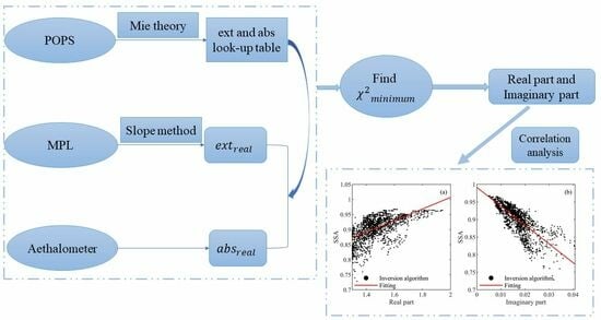
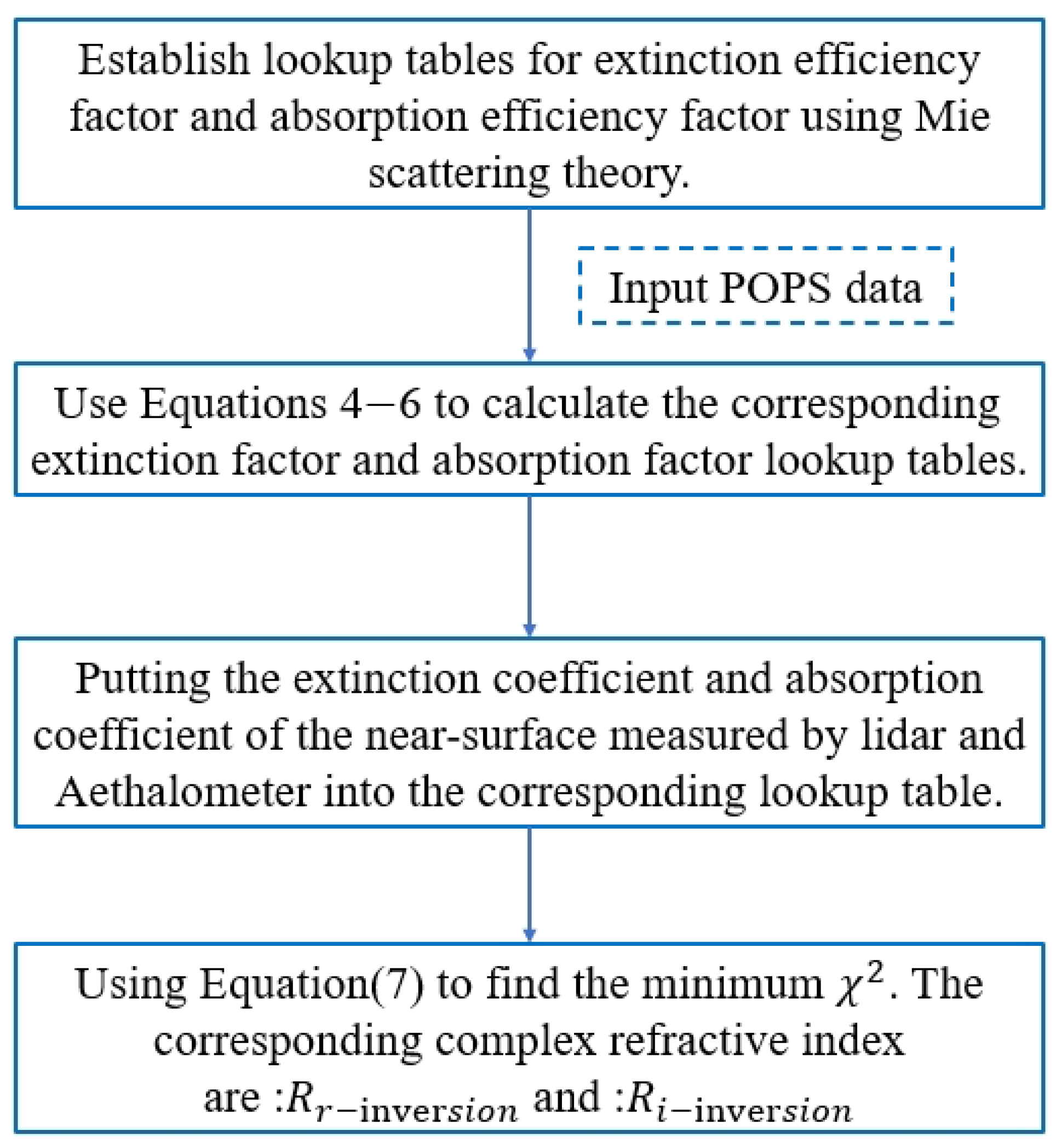
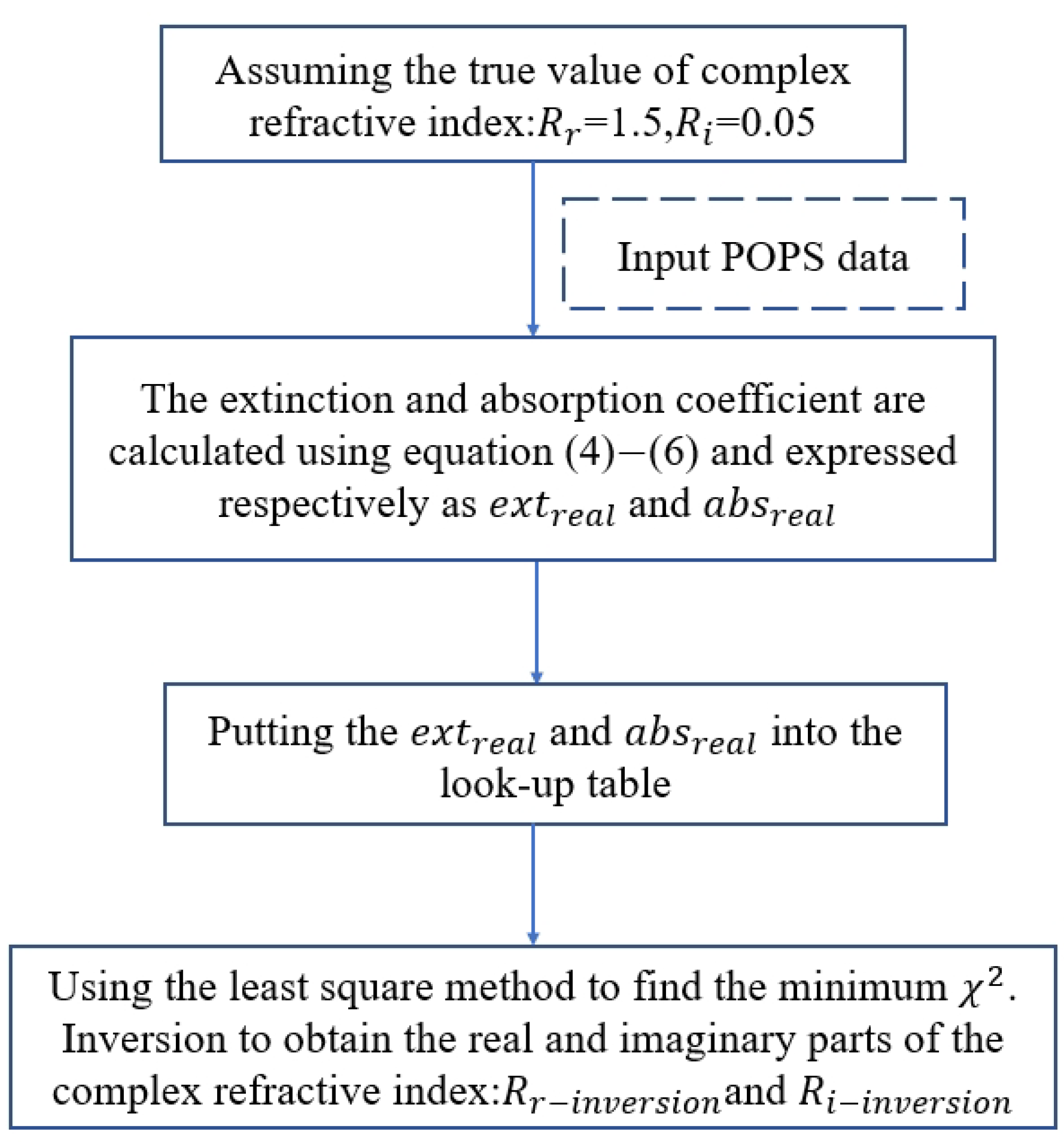
3.1. Introduction to Algorithms

The refractive index comprises two unknowns: the real and the imaginary parts. Therefore, two known quantities are essential to restrict the inversion. Since the real part of the complex refractive index is connected to scattering and the imaginary part is linked to absorption [21], the algorithm’s overall design utilizes the extinction coefficient (=scattering + absorption) determined by the MPL and the absorption coefficient measured by the Aethalometer as known values. It then employs the aerosol particle spectra measured by the POPS to determine the real and imaginary parts of the equivalent complex refractive index of the aerosol based on the theory of MIE scattering.
The POPS measures the aerosol concentration in each particle size channel. The extinction coefficient σ e x t , scattering coefficient σ s c a , and absorption coefficient σ a b s of the aerosol can be calculated using the Mie scattering theory. The corresponding formulas can be expressed as follows [40,41]:
σ e x t = r 1 r 2 π r 2 Q e x t ( m , r , λ ) n ( r ) d r
σ s c a = r 1 r 2 π r 2 Q s c a ( m , r , λ ) n ( r ) d r
σ e x t = σ s c a + σ a b s
where the extinction efficiency factor and backscattering efficiency factor of the aerosol particles are represented by Q e x t ( m , r , λ ) and Q s c a ( m , r , λ ) , respectively; m = n r i n i denotes the complex refractive index of the aerosol particles; n r stands for the real part of the refractive index; n i signifies the imaginary part of the refractive index; r is the radius of the aerosol particles; λ is the wavelength of the light; and n(r) denotes the spectral distribution of the aerosol particles.
To enhance computational efficiency, we constructed a lookup table for calculating extinction and scattering efficiency factors for various particle sizes and values of real and imaginary parts. The wavelength is 532 nm, and particle sizes are based on the POPS’s aerosol size binning. The real and imaginary parts of the refractive index refer to the actual aerosol situation. The range of the real part is 1.3–2.0 with a step size of 0.01, and the range of the imaginary part is 0.001–0.1 with a step size of 0.001. Based on the calculated look-up table and the measured spectral distribution of the particle sizes of the POPS, the correlative extinction and absorption coefficient lookup tables are computed based on Equations (4)–(6).
Once the look-up tables for extinction and absorption coefficients have been obtained, the least-squares method can be employed to minimize the error between the measured and theoretically calculated values of these coefficients to determine the optimal value for the complex refractive index. Theoretically, using two known numbers to solve for two unknowns is possible. Specifically, using the extinction and absorption coefficients at a given time during a coordinated observation, it is feasible to solve for the real and imaginary parts of the refractive index at that moment in time through the least-squares error method (single-point constraint method). Considering the inherent instrumental observation errors, this paper assumes that the aerosol source remains relatively stable for a certain period, indicating that the refractive index of the aerosol remains constant during this interval. The multi-point constraint method is adopted, which employs multi-point observation (N = 600) during this period to restrict the solution of the real part of the refractive index and the imaginary part (two unknowns) to minimize the impact of observation errors. The instrument has a resolution of 1 s, where N = 600 corresponds to a duration of ten minutes. The error function is defined as follows:
χ 2 ( n , k ) = 1 N i = 1 N i [ σ e x t , m e a s u r e d σ e x t , c a l c u l a t e d σ e x t , m e a s u r e d i 2 + σ a b s , m e a s u r e d σ a b s , c a l c u l a t e d σ a b s , m e a s u r e d i 2 ]
where χ 2 ( n , k ) represents the sum of squares of the fraction difference of extinction coefficient and absorption coefficient to their actual measured values, N is the number of measurements used in the retrieval, σ e x t , m e a s u r e d represents the extinction coefficient of near-surface aerosols obtained from horizontal measurements using MPL, σ e x t , c a l c u l a t e d denotes the extinction coefficient of the aerosol calculated using different combinations of complex refractive indices combined with Mie scattering theory, σ a b s , m e a s u r e d denotes the absorption coefficients of aerosols measured using an Aethalometer, and σ a b s , c a l c u l a t e d denotes the absorption coefficients of aerosols calculated using different combinations of complex refractive indices combined with Mie scattering theory.
In summary, the flowchart of the inversion algorithm is shown in Figure 2. Figure 3 depicts the graphs of extinction and absorption coefficients based on aerosol particle sizes measured by the POPS on 1 April 2022, where R r and R i represent the real and imaginary parts, respectively. From Figure 3 left, it is evident that there is a positive correlation between the extinction coefficient and the real part of the refractive index overall. When the imaginary part is less than or equal to 10 2 , the extinction coefficient is primarily determined by the real part of the refractive index. It is essentially unaffected by the imaginary part. When the imaginary part is greater than or equal to 10 2 , the extinction coefficient is still mainly influenced by the real part of the refractive index. However, it begins to demonstrate the effects of the imaginary component. As shown in Figure 3 right, the absorption coefficient exhibits a steadily increasing trend along with the complex refractive index’s real and imaginary parts. The real part moderately influences the absorption coefficient and is significantly influenced by the imaginary part. In conclusion, employing a method that uses a single variable constraint to invert either the real or imaginary part of the complex refractive index will result in errors. This is because the extinction and absorption coefficients are affected and changed by more than one variable. This indirectly verifies the advantage of using two variable constraints to invert the complex refractive index of aerosols.

3.2. Simulation Analysis

Since measuring the complex refractive index of aerosols in real-time and synchronously in the external field is challenging, this paper analyses and verifies the algorithm’s feasibility and reliability through simulation experiments. The purpose of the sensitivity study is to simulate possible sources of errors, including measurement errors of the MPL, Aethalometer, and POPS, in order to quantify the errors in the inverted near-ground atmospheric aerosol complex refractive index.
A study found that the aerosol complex refractive index obtained through inversion methods is very sensitive to uncertainties in the size distribution of particles [42]. In our simulation experiments, we initially considered errors from POPS measurements and compared previous inversion methods that use a single-point constraint. The specific steps of the simulation analysis are illustrated in Figure 4. Considering that the actual complex refractive index of atmospheric aerosols is unknown, we assume as a computational prerequisite that the real and imaginary parts of the complex refractive index of aerosols are constant over a specific time ( R r = 1.5 and R i = 0.05 ). We use the particle number concentration data measured by POPS as input and calculate the extinction and absorption coefficients at the time, denoted as e x t r e a l and a b s r e a l , respectively, using Formulas (4)–(6). We then input e x t r e a l and a b s r e a l into the lookup table and use the least squares method to find the smallest χ 2 . The corresponding complex refractive indices are denoted as R r i n v e r s i o n and R i i n v e r s i o n . Finally, we analyze the error between the assumed actual complex refractive index and the inverted equivalent complex refractive index.This article employs particle number concentrations measured by the POPS between 13:00 and 19:00 on 25 February to simulate a continuous period. The retrieval of the equivalent refractive index from the lookup table uses a multi-point constraint method, while a single-point constraint method is used concurrently for the inversion process.
Figure 5 shows box plots of the variation in the real and imaginary parts (the top and bottom edges of the box represent 75% and 25%, respectively, and the line in the box represents the median; the top and bottom represent the maximum and minimum values obtained from the inversion), which were obtained by using MATLAB’s random number function to add a random error of 1% to 10% to the raw number concentration of particles measured by the POPS and then inverted using the single-point constraint (blue line) and multi-point constraint methods (red line), where (a) and (b) represent the range of variation and error of the real and imaginary parts of the aerosol complex refractive index obtained by inversion using the two methods, respectively. From the Figure 5, with the increase in the instrumental error, the variation range of the inversion results of the two methods show a gradually increasing trend. It can also be seen that the inversion of the real part of the aerosol equivalent complex refractive index using multi-point constraints has a smaller error than that obtained by using single-point constraints, e.g., when the instrumental error of the POPS is at 5%, the relative maximum error ratio (RMER) of the real part obtained by using multi-point constraints and single-point constraints are 2% and 2.7%, respectively, and the RMER for the imaginary part is 10% and 12%, respectively. The formula is shown in Equation (8). It can be seen that the inversion using multi-point constraints is more advantageous than single-point constraints and can better eliminate part of the interference from the error of the instrumental observation data.
R M E R = m a x ( R i n v e r s i o n R r e a l R r e a l 100 % )
We further simulate the case where the MPL, the Aethalometer, and the POPS have measurement errors individually or simultaneously. The simulation experiment is set up with seven possible combinations of (1) particle spectra only, (2) extinction coefficient only, (3) absorption coefficient only, (4) extinction coefficient and absorption coefficient, (5) extinction coefficient and particle spectra, (6) absorption coefficient and particle spectra, and (7) all three instruments introduce errors. The simulation process is similar to Figure 4, except that the errors of the corresponding instruments are added according to different combinations in the simulation process; meanwhile, the errors of the instruments are all taken as 10% to check the performance of the algorithm in this paper when the instrument errors are large.
Figure 6 shows the box plots of the real and imaginary parts of the complex refractive index obtained using this paper’s algorithm for different combinations of cases when the instrumental errors are all considered to be 10%. From Figure 6, the RMER in the real part obtained by inversion is calculated to be 4%, and the RMER in the imaginary part is 20% when only the random measurement error of the particle spectrum is considered (case 1). Considering that the only random error in the extinction coefficient measurement is 10%, the inversion yields an RMER of 4.3% in the real part and 8% in the imaginary part (case 2). When the random error of the absorption coefficient measured by the Aethalometer is 10%, the inversion yields essentially no error in the real part and 16% in the imaginary part (case 3). When the random errors of both extinction and absorption coefficient measurements are 10%, the inversion yields less than 5% error in the real part and 24% RMER in the imaginary part (case 4). When the errors of extinction coefficient and particle spectrum measurements are 10%, the inversion yields an RMER of 8% in the real part and 28% in the imaginary part (case 5). When the errors of the absorption coefficient and particle spectrum measurements are 10%, the inversion yields an RMER of 4.7% in the real part and 24% in the imaginary part (case 6). When the random errors of all three instrumental measurements are 10%, the inversion yields an RMER of 8.7% in the real part and 34% in the imaginary part (case 7). In summary, the sensitivity study shows that the real part of the inversion is relatively insensitive to instrumental errors, with an overall error of less than 8.7% when an instrumental error of 10% is considered. In contrast, the imaginary part is relatively more sensitive to instrumental measurement errors. Figure 6 shows that when all three instruments bring a 10% error, the real and imaginary parts of the refractive index obtained using the algorithm produce a larger error range. In actual measurements, the measurement error of the POPS is around 5% [24], and the instrumental errors of both the MPL and Aethalometer are less than 10% [9], so the errors of the imaginary and real parts obtained from the actual measurement inversion should be much smaller than those in Figure 6.

3.3. Analysis of Inversion Results from Experimental Observations

This paper applies the algorithm to the measured data from March to April 2022 in the Hefei area for aerosol equivalent complex refractive index inversion. Due to the instability of the instrument during the experiment and the weather, data from 28 March to 4 April were selected for analysis after screening the experimental data for a total of one week (the quality of the MPL horizontal measurement data on 31 March was poor, so they were not used). Figure 7 shows the meteorological variations during the test period. From Figure 7a, we can see that each day, the temperature rises from around 6:00 to reach a maximum value around 14:00 and then starts to fall (except for the 31st of March), while the relative humidity (RH) varies in the opposite direction to the temperature. Figure 7b shows that wind speeds were generally low during the experiment, with maximum wind speeds not exceeding 3 m/s.
Figure 8 compares the extinction coefficient ( σ e x t , m e a s u r e d ) measured by the MPL and the extinction coefficient ( σ e x t , c a l c u l a t e d ) corresponding to the smallest χ 2 obtained using Equation (7). It can be seen that the range of variation in the extinction coefficient for one week is 0.1 to 1.2 km 1 . The extinction coefficient increased gradually from noon on March 30 to the early morning of the next day, reaching a high of around 1.2 km 1 . This indicates severe pollution on that day. Figure 9 shows that the coefficient of determination ( R 2 ) between the extinction coefficient obtained using the method provided in this study and that measured by the MPL is 0.998. The root mean square error (RMSE) is 0.0075 km 1 .
Figure 10 shows the comparison graph between the absorption coefficient ( σ a b s , m e a s u r e d ) observed by the Aethalometer and the absorption coefficient ( σ e x t , c a l c u l a t e d ) obtained when the minimum χ 2 is calculated using the lookup table. The change range of the absorption coefficient is from 0.01 to 0.08 km 1 . Figure 11 fits the actual measurements of the absorption coefficient and the simulated values calculated using Mie scattering theory, finding that their R 2 value is 0.991, and the RMSE is 2 × 10 4 km 1 . The correlation and error analysis shows that the extinction and absorption coefficients retrieved using the inversion algorithm have minimal errors and high correlations with the measured values.
Figure 12 demonstrates the changes over time in the equivalent complex refractive index of near-ground aerosols during the measurement period, as provided by the algorithm in this paper. The figure shows significant fluctuations in the real part of the complex refractive index of aerosols. The real part of the refractive index varied from 1.3 to 1.96 and the imaginary part from 0.005 to 0.041, with mean values of 1.48 and 0.017 for the real and imaginary parts, respectively. A study found that the average complex refractive index in the summer in the Hefei region was 1.5 i 0.016 , the average aerosol complex refractive index in Xinjiang in December 2015 was 1.5 i 0.01 , the average complex refractive index in Tianjin region in the summer of 2011 was 1.5 i 0.017 , and the average complex refractive index in Xiamen region in December 2006 was 1.52 i 0.008 [21]. Measurements of aerosols in the Paris region revealed an average complex refractive index of 1.51 ( ± 0.2 ) i 0.017 ( ± 0.003 ) at a wavelength of 532 nm [9]. Based on multi-wavelength backscattering and extinction measurements performed by a lidar system, the wavelength-independent complex refractive index of the aerosol was derived as 1.56 i 0.009 [43]. These research results show good consistency with the complex refractive index obtained by inversion through the algorithm in this study. In addition, it can be seen from Figure 12a that the partial real part obtained by the inversion is close to 1.3. Some studies also reported some unreasonably low values (real part less than 1.3) and gave possible explanations, such as inaccuracies in the retrieval method, non-analyzed biogenic particles, or non-spherical particles [44].
To verify the accuracy of the obtained near-surface aerosol equivalent refractive indices, the real and imaginary parts of the ACRI were correlated against the single-scattering albedo (SSA), respectively, as shown in Figure 13. A higher SSA indicates a stronger scattering ability of aerosols. Conversely, a lower SSA suggests a stronger absorption ability of aerosols.
Figure 13a shows the relationship between the real part of the effective refractive index of aerosols and the SSA obtained by the inversion algorithm in this study. Generally, the real part corresponds to scattering, and an increase in the real part indicates enhanced scattering, corresponding to a larger SSA. It can be observed from the figure that there is a relatively strong positive correlation between the real part of the aerosol refractive index and SSA. The relationship between the real part and SSA was obtained by fitting as ( R 2 = 0.36 , R M S E = 0.032 ):
y = 0.19 x + 0.62
Figure 13b depicts the relationship between the imaginary part of the aerosol equivalent complex refractive index and the SSA. Generally, an increase in the imaginary part indicates enhanced absorption, leading to a smaller SSA. It is evident from the graph that there exists a strong linear negative correlation between the inverted refractive index imaginary part and SSA. Through fitting, a functional relationship between the two is determined as follows ( R 2 = 0.64 , R M S E = 0.024 ):
y = 5.3 x + 0.99
In summary, the correlation analysis reveals a positive correlation between the real part and SSA and a good negative correlation between the imaginary part and SSA, which implies that the ACRI inversion method presented in this paper is valid or, at the very least, self-consistent.

4. Conclusions

The microphysical and optical properties of near-surface aerosols were measured jointly by an MPL, Aethalometer, and POPS near Dongpu Reservoir in the western suburb of Hefei from the end of March to the beginning of April 2022. The equivalent complex refractive index of the aerosols in Hefei was obtained based on the Mie scattering iterative algorithm, and the conclusions are as follows:
(1)
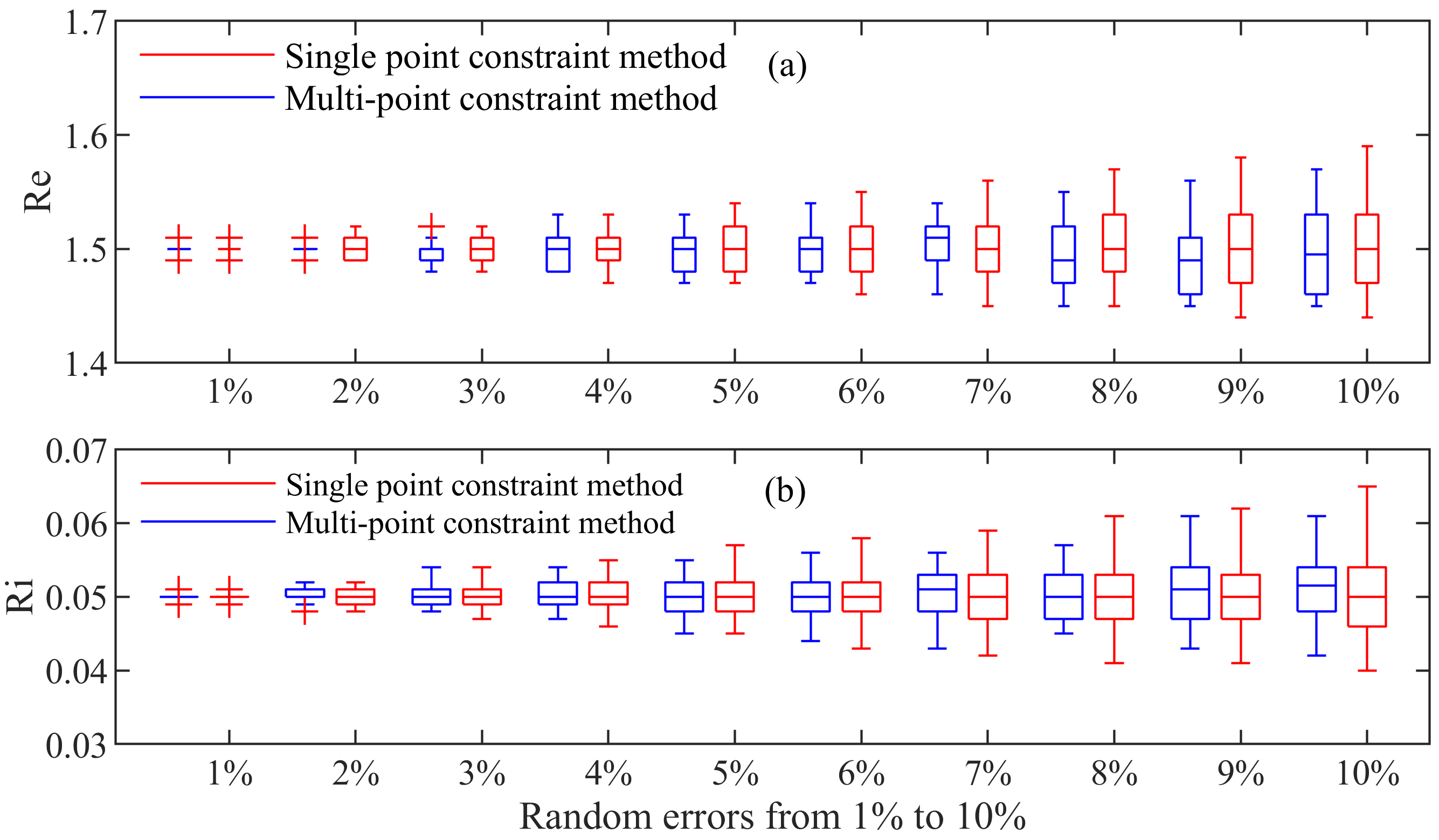
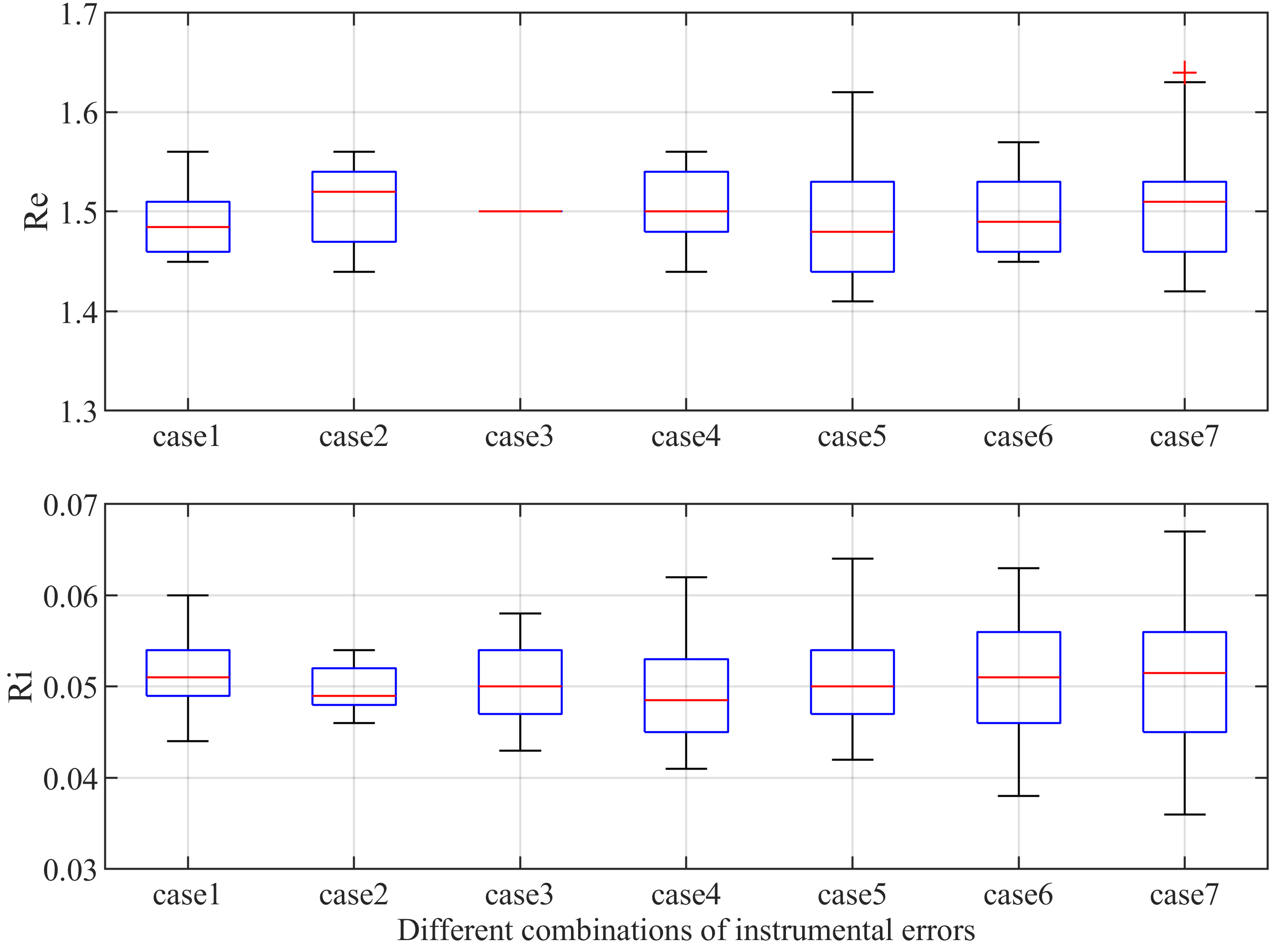
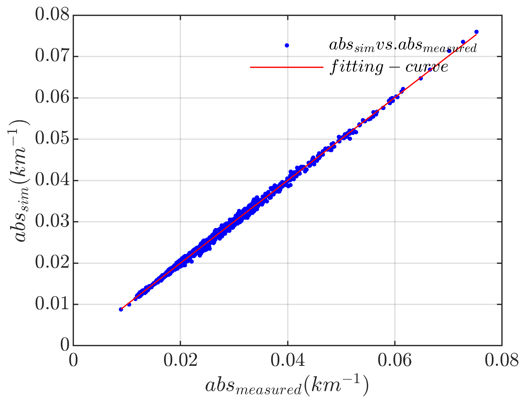
The reliability of the optimization algorithm for aerosol equivalent complex refractive index inversion was simulated. The results show that, compared with the single-point method, the multi-point constraint method is less sensitive to instrumental errors, can better eliminate the interference of some errors from the instrumental observation data, and the inversion results have better reliability than those of the single-point method.
(2)
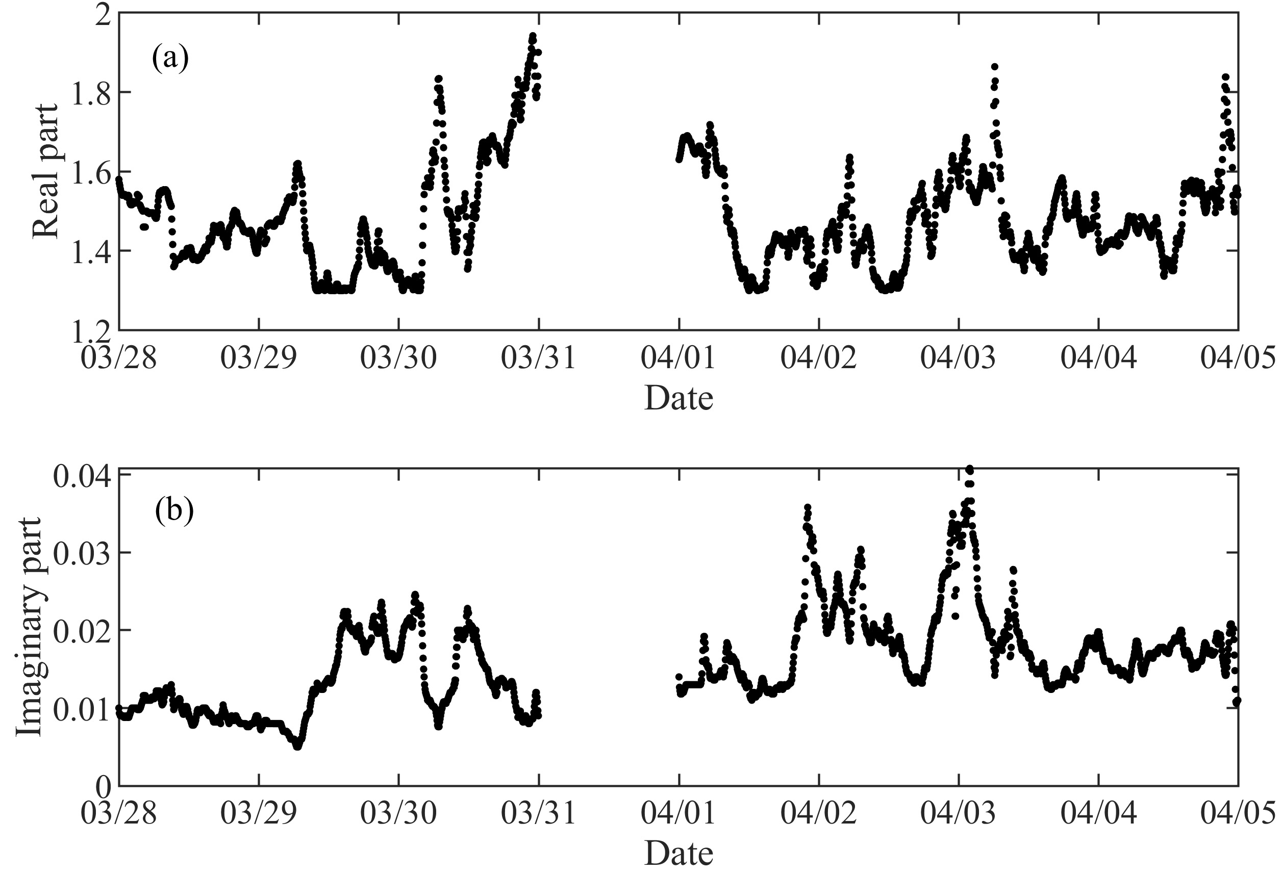
According to the retrieval results, the mean value of the equivalent refractive index of the aerosols observed during the test period is 1.48 − i0.017.
(3)
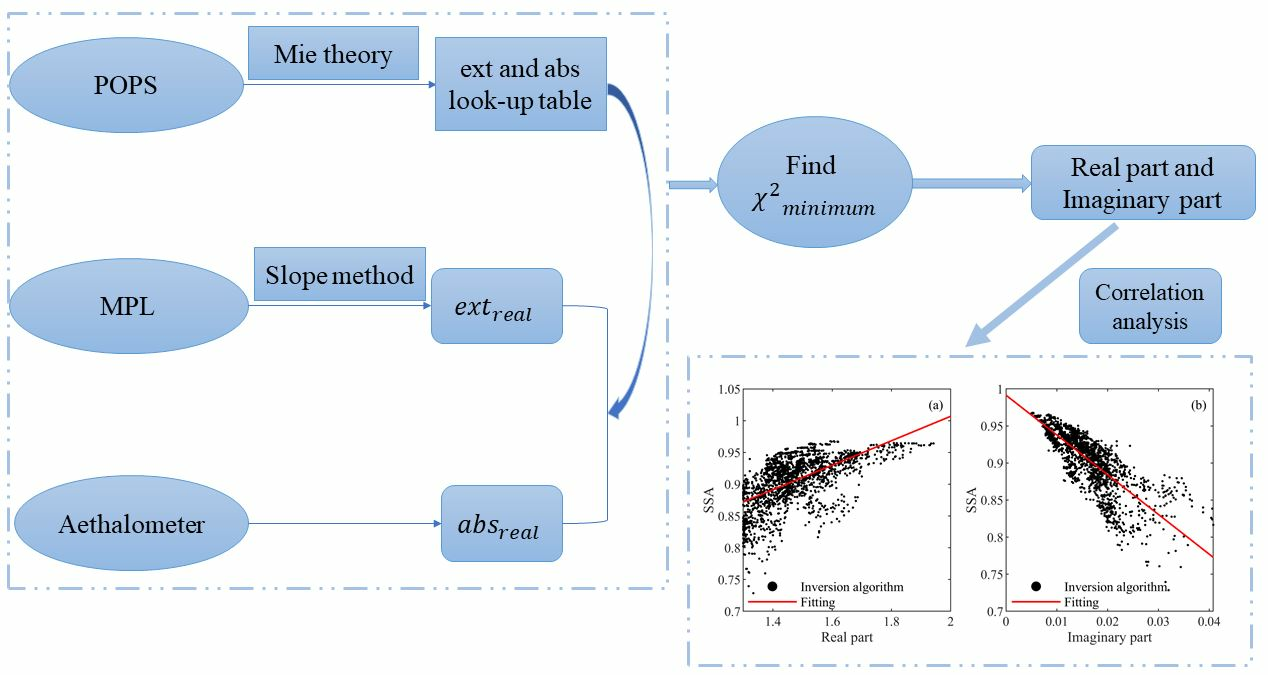
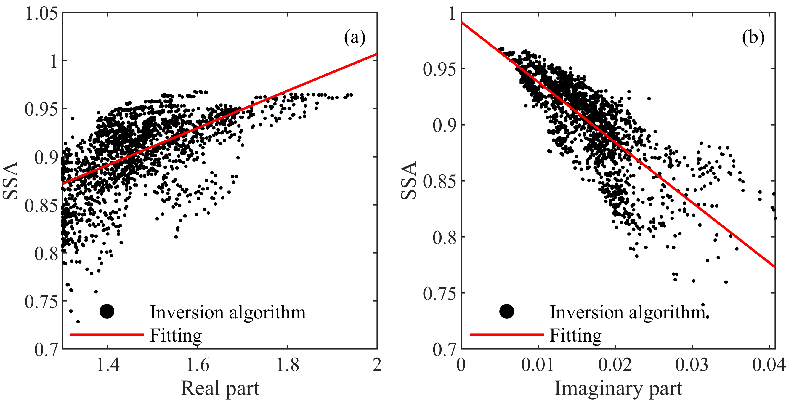
The correlation between the real and imaginary parts of the aerosol refractive index and SSA was analyzed. The results show a positive correlation ( y = 0.19 x + 0.62 ) between the real part and the SSA and a negative correlation ( y = 0.53 x + 0.99 ) between the imaginary part and the SSA.

Author Contributions

T.L. and X.L. conducted the experiments and conceived and designed the contents of this paper; Q.L., K.Z., C.L., N.L., J.C. and L.Z. contributed to the development of the analysis programs; X.M. performed data and visualization as well as formal analysis and wrote the manuscript; T.L. reviewed and edited the manuscript. All authors have read and agreed to the published version of the manuscript.

Funding

This research has been supported by the Natural Science Foundation of Anhui Province Outstanding Youth Program (2008085j19); the Advanced Laser Technology Laboratory of Anhui Province’s Foundation (AHL2021QN01); and the South Lake Light Laboratory Autonomous Research Program (22-NHLL-ZZKY-005).

Data Availability Statement

Data underlying the results presented in this paper are not publicly available at this time but may be obtained from the authors upon reasonable request.

Acknowledgments

We would like to thank all the observers who worked hard on the field campaign during this experiment, the anonymous reviewers for their useful comments, and the editors who provided assistance during the revision; all of them have been important in improving this manuscript.

Conflicts of Interest

The authors declare no conflicts of interest. The funders had no role in the design of the study; in the collection, analyses, or interpretation of the data; in the writing of the manuscript; or in the decision to publish the results.

References

  1. Lenoble, J. Atmospheric Radiative Transfer; Studies in Geophysical Optics and Remote Sensing; Deepak Publishing: Morar Gwalior, India, 1993; Available online: https://books.google.sk/books?id=WDBRAAAAMAAJ (accessed on 24 December 2023).
  2. Liousse, C.; Devaux, C.; Dulac, F.; Cachier, H. Aging of savanna biomass burning aerosols: Consequences on their optical properties. J. Atmos. Chem. 1995, 22, 1–17. [Google Scholar] [CrossRef]
  3. Tegen, I.; Fung, I. Contribution to the atmospheric mineral aerosol load from land surface modification. J. Geophys. Res. 1995, 100, 18707–18726. [Google Scholar] [CrossRef]
  4. World Health Organization; Regional Office for Europe. Health Aspects of Air Pollution: Results from the WHO Project “Systematic Review of Health Aspects of Air Pollution in Europe”; WHO Regional Office for Europe: Copenhagen, Denmark, 2004. [Google Scholar]
  5. IPCC. 2007: Climate Change 2007: Synthesis Report. Contribution of Working Groups I, II and III to the Fourth Assessment Report of the Intergovernmental Panel on Climate Change; Core Writing Team, Pachauri, R.K., Reisinger, A., Eds.; IPCC: Geneva, Switzerland, 2007; 104p. [Google Scholar]
  6. Liu, N.; Cui, S.; Luo, T.; Chen, S.; Yang, K.; Ma, X.; Sun, G.; Li, X. Characteristics of Aerosol Extinction Hygroscopic Growth in the Typical Coastal City of Qingdao, China. Remote Sens. 2022, 14, 6288. [Google Scholar] [CrossRef]
  7. Bluvshtein, N.; Flores, J.M.; Riziq, A.A.; Rudich, Y. An Approach for Faster Retrieval of Aerosols’ Complex Refractive Index Using Cavity Ring-Down Spectroscopy. Aerosol Sci. Technol. 2012, 46, 1140–1150. [Google Scholar] [CrossRef]
  8. Zhang, X.L.; Mao, M.; Chen, H.B. Characterization of optically effective complex refractive index of black carbon composite aerosols. J. Atmos. Sol.-Terr. Phys. 2020, 198, 105180. [Google Scholar] [CrossRef]
  9. Raut, J.C.; Chazette, P. Vertical profiles of urban aerosol complex refractive index in the frame of ESQUIF airborne measurements. Atmos. Chem. Phys. 2008, 8, 901–919. [Google Scholar] [CrossRef]
  10. Zhao, D.; Yin, Y.; Zhang, M.; Wang, H.; Lu, C.; Yuan, L.; Shi, S. The Optical Properties of Aerosols at the Summit of Mount Tai in May and June and the Retrieval of the Complex Refractive Index. Atmosphere 2020, 11, 655. [Google Scholar] [CrossRef]
  11. Zenkova, P.N.; Chernov, D.G.; Panchenko, M.V. Complex refractive index in the model of the vertical profile of aerosol optical characteristics in the troposphere of Western Siberia. Proc. SPIE 2022, 12341, 1234138. [Google Scholar] [CrossRef]
  12. Zhang, X.L.; Mao, M. Optically effective complex refractive index of coated black carbon aerosols: From numerical aspects. Atmos. Chem. Phys. 2019, 19, 7507–7518. [Google Scholar] [CrossRef]
  13. Guyon, P.; Boucher, O.; Graham, B.; Beck, J.; Mayol-Bracero, O.L.; Roberts, G.C.; Maenhaut, W.; Artaxo, P.; Andreae, M.O. Refractive index of aerosol particles over the Amazon tropical forest during LBA-EUSTACH 1999. J. Aerosol Sci. 2003, 34, 883–907. [Google Scholar] [CrossRef]
  14. Kandler, K.; Schütz, L.; Deutscher, C.; Ebert, M.; Hofmann, H.; Jäckel, S.; Jaenicke, R.; Knippertz, P.; Lieke, K.; Massling, A.; et al. Size distribution, mass concentration, chemical and mineralogical composition and derived optical parameters of the boundary layer aerosol at Tinfou, Morocco, during SAMUM 2006. Tellus B Chem. Phys. Meteorol. 2009, 61, 32–50. [Google Scholar] [CrossRef]
  15. Chazette, P.; Liousse, C. A case study of optical and chemical ground apportionment for urban aerosols in Thessaloniki. Atmos. Environ. 2001, 35, 2497–2506. [Google Scholar] [CrossRef]
  16. Stier, P.; Feichter, J.; Kinne, S.; Kloster, S.; Vignati, E.; Wilson, J.; Ganzeveld, L.; Tegen, I.; Werner, M.; Balkanski, Y.; et al. The aerosol-climate model ECHAM5-HAM. Atmos. Chem. Phys. 2005, 5, 1125–1156. [Google Scholar] [CrossRef]
  17. Dubovik, O.; Sinyuk, A.; Lapyonok, T.; Holben, B.N.; Mishchenko, M.; Yang, P.; Eck, T.F.; Volten, H.; Munoz, O.; Veihelmann, B.; et al. Application of spheroid models to account for aerosol particle nonsphericity in remote sensing of desert dust. J. Geophys. Res.-Atmos. 2006, 111, D11208. [Google Scholar] [CrossRef]
  18. Stock, M.; Cheng, Y.F.; Birmili, W.; Massling, A.; Wehner, B.; Müller, T.; Leinert, S.; Kalivitis, N.; Mihalopoulos, N.; Wiedensohler, A. Hygroscopic properties of atmospheric aerosol particles over the Eastern Mediterranean: Implications for regional direct radiative forcing under clean and polluted conditions. Atmos. Chem. Phys. 2011, 11, 4251–4271. [Google Scholar] [CrossRef]
  19. Schkolnik, G.; Chand, D.; Hoffer, A.; Andreae, M.O.; Erlick, C.; Swietlicki, E.; Rudich, Y. Constraining the density and complex refractive index of elemental and organic carbon in biomass burning aerosol using optical and chemical measurements. Atmos. Environ. 2007, 41, 1107–1118. [Google Scholar] [CrossRef]
  20. Riziq, A.A.; Erlick, C.; Dinar, E.; Rudich, Y. Optical properties of absorbing and non-absorbing aerosols retrieved by cavity ring down (CRD) spectroscopy. Atmos. Chem. Phys. 2007, 7, 1523–1536. [Google Scholar] [CrossRef]
  21. Geng, M.; Li, X.B.; Qin, W.B.; Liu, Z.Y.; Lu, X.Y.; Dai, C.M.; Miao, X.K.; Weng, N.Q. Research on the characteristics of aerosol size distribution and complex refractive index in typical areas of China. Infrared Laser Eng. 2018, 47, 191–197. [Google Scholar] [CrossRef]
  22. Zhang, X.L.; Mao, M.; Yin, Y. A Numerical Study of Dependencies of Aerosol Scattering and Absorption on Its Refractive Index. Chin. J. Light Scatt. 2017, 29, 102–106. [Google Scholar] [CrossRef]
  23. Mueller, D.; Weinzierl, B.; Petzold, A.; Kandler, K.; Ansmann, A.; Mueller, T.; Tesche, M.; Freudenthaler, V.; Esselborn, M.; Heese, B.; et al. Mineral dust observed with AERONET Sun photometer, Raman lidar, and in situ instruments during SAMUM 2006: Shape-independent particle properties. J. Geophys. Res.-Atmos. 2010, 115, D11207. [Google Scholar] [CrossRef]
  24. Gao, R.S.; Telg, H.; McLaughlin, R.J.; Ciciora, S.J.; Watts, L.A.; Richardson, M.S.; Schwarz, J.P.; Perring, A.E.; Thornberry, T.D.; Rollins, A.W.; et al. A light-weight, high-sensitivity particle spectrometer for PM2.5 aerosol measurements. Aerosol Sci. Technol. 2015, 50, 88–99. [Google Scholar] [CrossRef]
  25. Chen, S.S.; Xu, Q.S.; Xu, C.D.; Yu, D.S.; Chen, X.W. Calculation of Whole Atmospheric Aerosol Optical Depth Based on Micro-Pulse Lidar. Acta Opt. Sin. 2017, 37, 17–25. [Google Scholar] [CrossRef]
  26. Xiong, X.L.; Jiang, L.H.; Feng, S. Mie scattering lidar echo signal processing methods. Infrared Laser Eng. 2012, 41, 89–95. [Google Scholar]
  27. Kunz, G.J.; de Leeuw, G. Inversion of lidar signals with the slope method. Appl. Opt. 1993, 32, 3249–3256. [Google Scholar] [CrossRef] [PubMed]
  28. Klett, J.D. Lidar inversion with variable backscatter/extinction ratios. Appl. Opt. 1985, 24, 1638–1643. [Google Scholar] [CrossRef]
  29. Xiong, X.L.; Jiang, L.H.; Feng, S. Return signals processing method of Mie scattering lidar. Infrared Laser Eng. 2012, 41, 89–95. [Google Scholar]
  30. Drinovec, L.; Mocnik, G.; Zotter, P.; Prevot, A.S.H.; Ruckstuhl, C.; Coz, E.; Rupakheti, M.; Sciare, J.; Mueller, T.; Wiedensohler, A.; et al. The “dual-spot” Aethalometer: An improved measurement of aerosol black carbon with real-time loading compensation. Atmos. Meas. Tech. 2015, 8, 1965–1979. [Google Scholar] [CrossRef]
  31. Healy, R.M.; Sofowote, U.; Su, Y.; Debosz, J.; Noble, M.; Jeong, C.H.; Wang, J.M.; Hilker, N.; Evans, G.J.; Doerksen, G.; et al. Ambient measurements and source apportionment of fossil fuel and biomass burning black carbon in Ontario. Atmos. Environ. 2017, 161, 34–47. [Google Scholar] [CrossRef]
  32. Bond, T.C.; Doherty, S.J.; Fahey, D.W.; Forster, P.M.; Berntsen, T.; DeAngelo, B.J.; Flanner, M.G.; Ghan, S.; Kärcher, B.; Koch, D.; et al. Bounding the role of black carbon in the climate system: A scientific assessment. J. Geophys. Res. Atmos. 2013, 118, 5380–5552. [Google Scholar] [CrossRef]
  33. Sokolik, I.N.; Toon, O.B. Incorporation of mineralogical composition into models of the radiative properties of mineral aerosol from UV to IR wavelengths. J. Geophys. Res. Atmos. 1999, 104, 9423–9444. [Google Scholar] [CrossRef]
  34. Claquin, T.; Schulz, M.; Balkanski, Y.J. Modeling the mineralogy of atmospheric dust sources. J. Geophys. Res. Atmos. 1999, 104, 22243–22256. [Google Scholar] [CrossRef]
  35. Andreae, M.O.; Gelencsér, A. Black carbon or brown carbon? The nature of light-absorbing carbonaceous aerosols. Atmos. Chem. Phys. 2006, 6, 3131–3148. [Google Scholar] [CrossRef]
  36. Samset, B.H.; Stjern, C.W.; Andrews, E.; Kahn, R.A.; Myhre, G.; Schulz, M.; Schuster, G.L. Aerosol Absorption: Progress Towards Global and Regional Constraints. Curr. Clim. Chang. Rep. 2018, 4, 65–83. [Google Scholar] [CrossRef] [PubMed]
  37. Lu, H.; Wei, W.S.; Wu, X.P.; Cao, X.; Tang, X.L. An Approach to Decouple Aerosol Absorption Coefficients Using Aethalometer Observational Data. Desert Oasis Meteorol. 2011, 5, 36–39. [Google Scholar]
  38. Kirchstetter, T.W.; Novakov, T.; Hobbs, P.V. Evidence that the spectral dependence of light absorption by aerosols is affected by organic carbon. J. Geophys. Res. Atmos. 2004, 109, 21208. [Google Scholar] [CrossRef]
  39. Bergstrom, R.W.; Russell, P.B.; Hignett, P. Wavelength Dependence of the Absorption of Black Carbon Particles: Predictions and Results from the TARFOX Experiment and Implications for the Aerosol Single Scattering Albedo. J. Atmos. Sci. 2002, 59, 567–577. [Google Scholar] [CrossRef]
  40. Tao, Z.M.; Zhang, Y.C.; Zhang, G.X. Studies on Extinction efficiency factor properties of aerosol particle and the fit of size distribution. Chin. J. Quantum Electron. 2004, 21, 103–109. [Google Scholar]
  41. Xu, J.W.; Liu, D.; Xie, C.B.; Wang, Z.Z.; Wang, B.X.; Zhong, Z.Q.; Ma, H.; Wang, Y.J. Multi-Wavelength Fitting Simulation and Inversion of Atmospheric Aerosol Spectrum Distribution. Acta Opt. Sin. 2017, 37, 50–56. [Google Scholar] [CrossRef]
  42. Mack, L.A.; Levin, E.J.T.; Kreidenweis, S.M.; Obrist, D.; Moosmüller, H.; Lewis, K.A.; Arnott, W.P.; McMeeking, G.R.; Sullivan, A.P.; Wold, C.E.; et al. Optical closure experiments for biomass smoke aerosols. Atmos. Chem. Phys. 2010, 10, 9017–9026. [Google Scholar] [CrossRef]
  43. Muller, D.; Ansmann, A.; Wagner, F.; Franke, K.; Althausen, D. European pollution outbreaks during ACE 2: Microphysical particle properties and single-scattering albedo inferred from multiwavelength lidar observations. J. Geophys. Res.-Atmos. 2002, 107, AAC 3-1–AAC 3-11. [Google Scholar] [CrossRef]
  44. Virkkula, A.; Koponen, I.K.; Teinila, K.; Hillamo, R.; Kerminen, V.M.; Kulmala, M. Effective real refractive index of dry aerosols in the Antarctic boundary layer. Geophys. Res. Lett. 2006, 33, 6805. [Google Scholar] [CrossRef]
Figure 1. The red pentagram in the picture represents the experimental site.
Remotesensing 16 00279 g001
Figure 2. Flow chart of the inverse equivalent complex refractive index algorithm.
Remotesensing 16 00279 g002
Figure 3. (left) The trend of extinction coefficient with complex refractive index; (right) the trend of absorption coefficient with complex refractive index.
Remotesensing 16 00279 g003
Figure 4. Flowchart of the simulation analysis.
Remotesensing 16 00279 g004
Figure 5. POPS with random errors of 1% to 10% added to obtain box plots using single-point constraint and multi-point constraint inversion methods, respectively. (a) The range of variation in the real part of the complex refractive index obtained by inversion; (b) the range of variation in the imaginary part of the complex refractive index obtained by the inversion.
Remotesensing 16 00279 g005
Figure 6. (top) The range of variation in the real part obtained by inversion for different combinations of instrumental errors (the upper and lower sides of the blue line represent the 75 percentile and 25 percentile, respectively, and the red line represents the median). (bottom) The range of variation in the imaginary part obtained by inversion for different combinations of instrumental errors.
Remotesensing 16 00279 g006
Figure 7. Changes in temperature, humidity (a), and wind speed and direction (b) over time during the test period.
Remotesensing 16 00279 g007
Figure 8. Comparison of extinction coefficients obtained from MPL measurements and inversion algorithms (the black scattered points (Measured) in the figure represent the change curve of the extinction coefficient measured by the MPL during the measurement period, and the red solid line (Sim) is the change curve of the extinction coefficient obtained from the lookup table by employing the methodology proposed in this study).
Remotesensing 16 00279 g008
Figure 9. Fitting of measured and simulated values of extinction coefficients using Mie scattering theory.
Remotesensing 16 00279 g009
Figure 10. Comparison of absorption coefficients obtained using the Aethalometer and using the algorithm (the black scatter points (Measured) in the figure represent the variation curve of the absorption coefficient measured by the Aethalometer during the observation period, and the red solid line (Sim) represents the change curve of the absorption coefficient obtained using the algorithm proposed in this study).
Remotesensing 16 00279 g010
Figure 11. Fitting of measured and simulated values of absorption coefficients using Mie scattering theory.
Remotesensing 16 00279 g011
Figure 12. Complex refractive index of the aerosol during the measurement period obtained based on a look-up table optimization algorithm. (a) Evolution of the real part over time; (b) evolution of the imaginary part over time.
Remotesensing 16 00279 g012
Figure 13. (a) Correlation analysis of the real part and SSA obtained by inversion; (b) Correlation analysis of the imaginary part and the SSA obtained by inversion.
Remotesensing 16 00279 g013
Table 1. Binning radius of POPS (nm).
Bin12345678910111213141516
Lower1151251351501651852102503504755758551220153019902585
Upper12513515016518521025035047557585511201530199025853370
Disclaimer/Publisher’s Note: The statements, opinions and data contained in all publications are solely those of the individual author(s) and contributor(s) and not of MDPI and/or the editor(s). MDPI and/or the editor(s) disclaim responsibility for any injury to people or property resulting from any ideas, methods, instructions or products referred to in the content.

