Article

Lightweight-VGG: A Fast Deep Learning Architecture Based on Dimensionality Reduction and Nonlinear Enhancement for Hyperspectral Image Classification

1
Key Laboratory of Grain Information Processing and Control, Henan University of Technology, Ministry of Education, Zhengzhou 450001, China
2
Henan Key Laboratory of Grain Photoelectric Detection and Control, Henan University of Technology, Zhengzhou 450001, China
3
School of Artificial Intelligence and Big Data, Henan University of Technology, Zhengzhou 450001, China
4
Jiangsu Collaborative Innovation Center of Atmospheric Environment and Equipment Technology (CICAEET), Nanjing University of Information Science and Technology, Nanjing 210044, China
*
Author to whom correspondence should be addressed.
Remote Sens. 2024, 16(2), 259; https://doi.org/10.3390/rs16020259
Submission received: 13 November 2023 / Revised: 5 January 2024 / Accepted: 8 January 2024 / Published: 9 January 2024
(This article belongs to the Special Issue Deep Learning for the Analysis of Multi-/Hyperspectral Images II)

Abstract

:
In the past decade, deep learning methods have proven to be highly effective in the classification of hyperspectral images (HSI), consistently outperforming traditional approaches. However, the large number of spectral bands in HSI data can lead to interference during the learning process. To address this issue, dimensionality reduction techniques can be employed to minimize data redundancy and improve HSI classification performance. Hence, we have developed an efficient lightweight learning framework consisting of two main components. Firstly, we utilized band selection and principal component analysis to reduce the dimensionality of HSI data, thereby reducing redundancy while retaining essential features. Subsequently, the pre-processed data was input into a modified VGG-based learning network for HSI classification. This method incorporates an improved dynamic activation function for the multi-layer perceptron to enhance non-linearity, and reduces the number of nodes in the fully connected layers of the original VGG architecture to improve speed while maintaining accuracy. This modified network structure, referred to as lightweight-VGG (LVGG), was specifically designed for HSI classification. Comprehensive experiments conducted on three publicly available HSI datasets consistently demonstrated that the LVGG method exhibited similar or better performance compared to other typical methods in the field of HSI classification. Our approach not only addresses the challenge of interference in deep learning methods for HSI classification, but also offers a lightweight and efficient solution for achieving high classification accuracy.

1. Introduction

As a potent remote sensing technique, hyperspectral imaging might capture high-dimensional data about the Earth’s surface or other objects [1,2,3]. Unlike traditional remote sensing, which captures only a few broad spectral bands, hyperspectral imaging measures the reflectance or emission of light by spanning hundreds of contiguous and narrow spectral bands. These bands come from the shortwave-infrared, near-infrared, and visible sections of the electromagnetic spectrum. The resulting hyperspectral images (HSIs) contain plenty of information about the composition of materials on the surface that can be used in diverse applications, such as vegetation research, ocean exploration, mineral exploration, and disaster response. By analyzing the spectral signatures of various materials, hyperspectral imaging can be used to assist in the identification and mapping of different land cover types, such as forests, wetlands, urban areas, impervious (nonporous) surfaces, and agricultural fields [4,5,6,7].
In recent decades, many methods relying on artificial features have been developed [8,9,10,11,12]. However, artificial feature extraction is often constrained by domain-specific knowledge and expertise, making it challenging to adapt to different datasets and applications, and it lacks sufficient adaptability [13].
Unlike traditional images, remote sensing image data typically contains more dimensions. With the increase in data dimensionality, classifier performance often shows an initial improvement, because the added dimensions provide more information, enabling the classifier to better distinguish between different categories. However, as dimensionality continues to increase, performance eventually reaches a saturation point, where classification accuracy no longer improves and may even slightly decrease. This suggests that adding dimensions no longer provides useful information after, and may actually introduce noise or redundancy; this is referred to as the Hughes Phenomenon [14]. Therefore, dimensionality reduction is necessary to mitigate the effects of the dimensionality curse.
For remote sensing images, several dimensionality reduction methods have been presented, which can be broadly classified into two categories: feature extraction [15] and band selection [16].
Representative feature extraction methods include principal component analysis (PCA), independent component analysis, and linear discriminant analysis [17,18], among others. With the advancement of computer technology, supervised classification methods have evolved in sophistication. Supervised classification utilizes labeled sample data to train classification models or algorithms, such as support vector machines (SVM) [19] and random forests [20]. These models and algorithms enable the automatic classification of different land cover categories, and also have achieved significant improvements in accuracy and efficiency.
The rise of deep learning methods signifies a significant advancement in remote sensing image classification. Deep learning methods, particularly convolutional neural networks (CNNs) [21,22,23,24,25], exhibit excellent performance in image classification. Notably, they have the ability to automatically extract high-level features from remote sensing images without the need for complex feature engineering. This results in increased accuracy in remote sensing image classification. Furthermore, there are also methods that combine transformers and CNNs for HSI classification [26,27,28,29,30,31]. Deep learning models, especially CNNS, can automatically learn features from raw data. This means that there is no need for manual feature engineering, and that the model itself can discover the most important features. In contrast, SVM typically requires manual feature selection and extraction [32].
Band selection (BS) can help remove redundant spectral bands, thereby reducing the dimensionality of the HSI data. Furthermore, this can decrease computational costs, accelerate model training speed, and mitigate the risk of overfitting. Feature extraction also allows the model to automatically extract advanced features, while BS assists in selecting spectral bands relevant to the task. By integrating these two approaches, it is possible to achieve comprehensive use of the rich information in the HSI data. This includes various spectral features of the original data, as well as domain knowledge related to the task. This helps improve the model’s representational capacity and performance.
Harnessing the capabilities of these recent advances in technology, we propose a novel lightweight network architecture for HSI classification based on Visual Geometry Group (VGG) networks [33] and the incorporation of dimensionality reduction and multi-layer perceptron (MLP). In this method, we performed band selection to eliminate duplicate or redundant bands. Prioritizing band selection allowed us to identify the most relevant bands for classification. Furthermore, by using PCA dimensionality reduction, not only was the impact of noise reduced, but the amount of training data was reduced as well. These data preprocessing also improved the efficiency of subsequent network training and increased classification accuracy.
The contributions of this paper can be summarized as follows:
  • We simultaneously used band selection and whitened PCA to relieve the impact of random seeds on experimental results;
  • We propose a novel lightweight-VGG (LVGG) network architecture for HSI classification, which aims to maintain high performance while reducing the complexity and computational resource requirements of the network, enabling efficient HSI classification even in resource-constrained environments;
  • Our proposed method achieved better accuracy in three publicly available HSI datasets as compared to several other existing methods.
The remainder of this paper is organized as follows: Section 2 describes some related data preprocessing studies. In Section 3, the proposed LVGG network is introduced in detail. Section 4 introduces three publicly available HSI datasets and divides them into three parts (i.e., training, validation, and test sets). Section 5 analyzes comparative experimental results on three HSI datasets, and demonstrates the effectiveness of our method. Finally, some conclusions and discussions are provided in Section 6.

2. Related Work

2.1. Patch-Based Classification

In recent years, deep learning has experienced significant growth, and has had a profound impact on multiple domains, particularly in the field of hyperspectral image (HSI) classification, which is relevant to many deep learning-based models reaching widespread application. Models, such as autoencoders [34] and recurrent neural networks [35], have been extensively employed. Previously to this, CNNs, known for their local receptive fields and translational invariance, were most effective at feature extraction, thereby enhancing classification accuracy.
In HSI classification, various classification frameworks and architectures have been proposed to acquire spatial features and train classifiers. These frameworks often involve generating patches centered around sample pixels from an original image, which are then employed for feature extraction and classification using different network architectures. Some studies have introduced end-to-end networks that take 3D patches as inputs and produce specific labels for each patch using the last fully connected (FC) layer [36]. Other approaches have employed 2D CNNs with 1 × 1 convolution kernels and global average pooling to extract spectral information and prevent overfitting [37]. Neural networks with band-adaptive, spectral–spatial feature learning have also been proposed to solve the dimensionality curse and the spatial variability problems of spectral signatures. Additionally, deeper and wider networks with residual learning have been suggested, such as the contextual deep CNN, which utilizes multi-scale filter banks to simultaneously process spectral–spatial information [38].
To improve the aggregation of spectral–spatial information, researchers have introduced two-stream CNN-based architectures [39,40]. Before fusing the outputs for classification, these architectural designs employ 2D CNNs and other algorithms for the extraction of spatial and spectral information, respectively. Another category of spectral–spatial-based CNN architecture uses 3D CNNs to extract joint spectral–spatial features for HSI classification [36,41]. The spectral–spatial residual network (SSRN) [42], alternatively, utilizes residual blocks to learn spectral and spatial information in hyperspectral images. This enables the model to enhance its ability to identify different land cover categories and features. A fast and dense spectral–spatial convolution architecture has also been proposed [20], which uses different scales of 3D convolution and residual structures to learn spectral and spatial information. Another approach employs a hybrid convolution network that utilizes 3D convolution followed by 2D convolution to learn spectral–spatial features [21].
In recent years, various attention mechanisms have been integrated to enhance classification performance in the field of HSI classification [43]. These attention mechanisms enable models to dynamically focus on the most relevant and information-rich parts of an image, thereby improving classification accuracy [44]. One common type of attention module is the Squeeze-and-Excitation module [45], which generates channel attention vectors through global pooling and fully connected layers; these vectors are then used to recalibrate the responses of spectral features. Additionally, many spatial attention modules and channel attention modules are used in convolutional networks to enhance spectral and spatial features [46,47]. Furthermore, a double-branch dual-attention (DBDA) mechanism network is employed, incorporating both position attention modules and channel attention modules [24] to enhance the feature representations of remote sensing images. Thus, the above attention mechanisms have significantly improved the performance of remote sensing image classification methods and have enabled models to better adapt to the characteristics of different images and scenes.
In stark contrast to CNNs, transformers segment images into non-overlapping blocks, often referred to as tokens, and then pass these blocks as input sequences to the model. Transformers use attention mechanisms to learn the relationships between these blocks, and thus primarily model global information. As a result, they require substantial amounts of data for training. Recently, transformer models have also been employed for HSI classification and achieved good results. For instance, an improved transformer-based, spatial–spectral feature extraction method has previously been proposed as a means to obtain features [48]. Another study used a partial partition restore module to introduce a novel local transformer [27]. A spectral–spatial feature tokenization transformer (SSFTT) has also been developed to excavate spectral–spatial features and high-level semantic features [28].
As the vision transformer has gained popularity in computer vision, researchers have begun to explore its potential for HSI classification. However, compared to its application in natural image processing, the transformer model is not always as effective for remote sensing image classification. Some reasons for this include: (1) single viewpoints; remote sensing images are mostly captured from a top-down perspective, while natural images exhibit diverse viewpoint. (2) Limited background and objects; remote sensing images typically consist of specific land cover types, with the spatial distribution of objects often influenced by geographical information. Thus, neighboring regions may not have significant correlations. As a result, capturing global features may not be as meaningful, and local features become more crucial. Therefore, transformers may not offer substantial improvements over CNNs, and may even be less effective than CNNs in this context.

2.2. Dimensionality Reduction

Feature extraction and band selection are two commonly employed techniques for reducing dimensionality in hyperspectral data processing. The primary objective of these methods is to enhance data analysis and processing efficiency by reducing overall data dimensionality [49].
Feature extraction is a fundamental process in data analysis and machine learning. It involves selecting and transforming relevant information from raw data to create a more compact and informative representation, making it easier for algorithms to process and analyze the data. Feature extraction is used to reduce the dimensionality of data while retaining essential information. It simplifies data, making it more manageable and often improving the performance of machine learning algorithms. This transformation helps to more effectively capture the relevant characteristics present in the data. Common feature extraction methods include PCA and linear discriminant analysis, among others. These methods employ mathematical transformations to identify the most significant features within the data, thereby facilitating improved classification or analysis [50].
Band selection plays a pivotal role in remote sensing image processing, enabling the selection and extraction of the most informative spectral bands, rendering remote sensing data more amenable to analysis and interpretation. This process helps reduce computational complexity, improve classification accuracy, decrease storage requirements, and better cater to the specific needs of remote sensing applications. Optimal band selection enhances the richness of information in remote sensing imagery, offering critical support for precise land cover classification, monitoring, and analysis. Common band selection methods include ranking-based approaches, such as correlation coefficients and information gain, as well as clustering-based methods. Ranking methods sort bands based on their correlation or information content and select the top-ranked bands, while clustering methods group similar bands together and then select representative bands from each group for subsequent processing [51].
In a previous study, an improved, fast peak-based clustering method was introduced, which takes into account both intra-cluster distance and local density to rank bands. In the literature [52], an adaptive and distance-based band hierarchy clustering method was introduced by using the same ranking approach. Additionally, a fast neighborhood grouping band selection method [53] was proposed, which employs a coarse-to-fine grouping strategy to reduce redundancy, and then utilizes the product of information entropy and local density to rank bands.
Here, we introduce a preprocessing method for dimensionality reduction based on feature extraction and band selection, followed by the application of a deep learning network for HSI classification. First, a combined feature extraction and band selection approach was designed to extract valuable information for dimensionality reduction. An improved, lightweight-VGG architecture is then proposed for classification.

3. Proposed Method

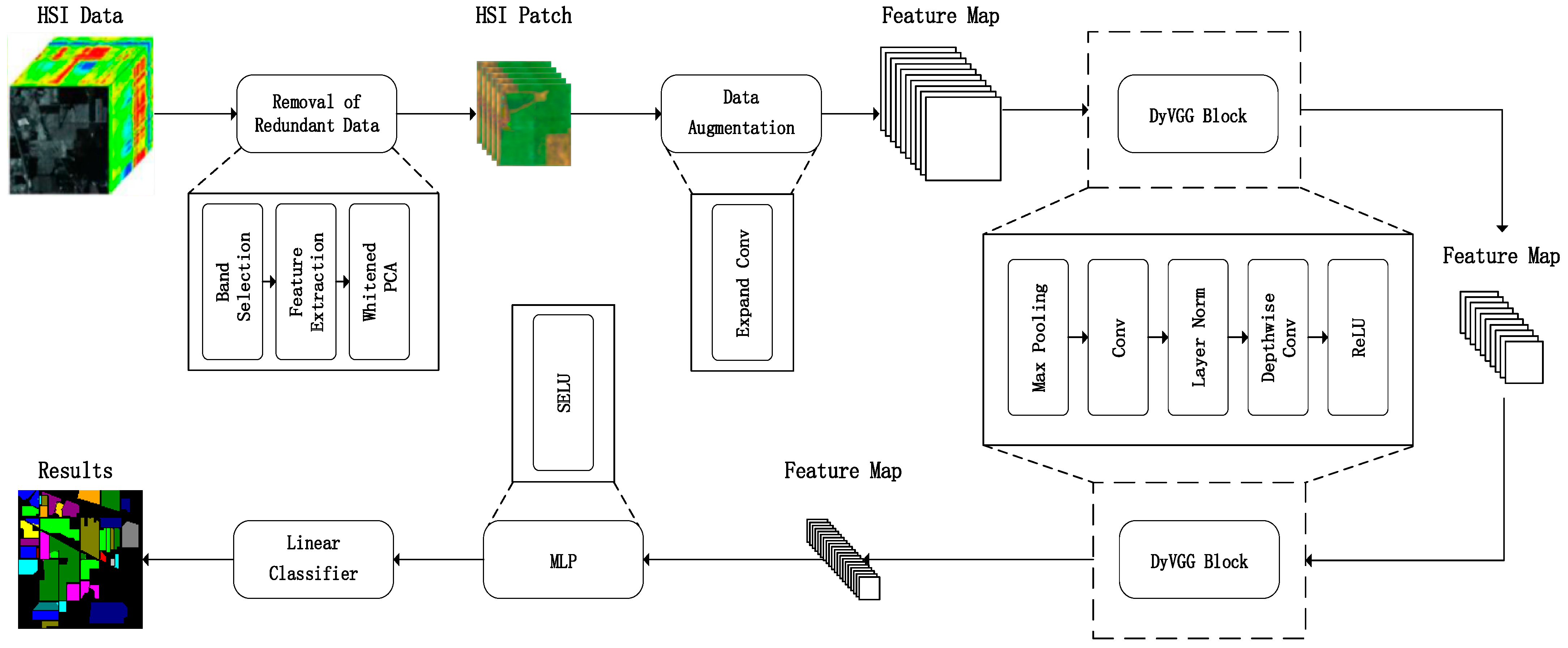
The workflow of the proposed lightweight-VGG method is depicted in Figure 1 and encompasses four primary stages. In this method, dimensionality reduction preprocessing is performed on the original HSI data. Next, an expand convolution is introduced to increase the network’s capacity, enabling the network to capture more data features, thus enhancing its performance. The dimension-enhanced data is then fed into a DyVGG block for patch-level feature extraction, and the extracted features are inputted into MLP and linear classifier layers to obtain the predicted labels of the sample data.

3.1. The Removal of Redundant Data

In HSI preprocessing, band selection is an effective way of filtering out redundant bands while retaining important information relevant to the target task. Additionally, PCA is usually used to further reduce the impact of noise and extract key feature information. Hence, we propose a redundant data removal method that integrates band selection and PCA.

3.1.1. Band Selection

This passage describes a process for grouping neighboring bands in a dataset represented by X . The bands in X , denoted as C bands, are initially divided into K equal groups. Each group, labeled X k (where k = 1, …, K ), is defined as follows:
X k = { X k 1 C K + 1 ,   ,   X k C K }   k [ C / K ] C { X k 1 C K + 1 ,   ,   X C }   k [ C / K ] > C
where X i represents the i-th band image of X and [ C / K ] represents the smallest integer greater than or equal to C / K .
Next, a fine partition algorithm [53] is applied to each of the initial band groups X k ( k = 1, …, K ) to create new band groups X k ( k = 1, …, K ). In this new partition, the number of bands may not be the same for different groups, and it is thus designed to group highly correlated spectral bands together, thereby resulting in lower correlation between the different band groups. For simplicity in this description, the new band groups are still marked with X k ( k = 1, …, K ), so the final grouping representation of X is given by:
X = { X 1 , X 2 , , X K }
These highly correlated spectral bands are grouped together, resulting in lower correlation between band groups. Therefore, selecting representative bands from each band group becomes a more reasonable approach. For each band group, we utilize correlation coefficients to find a representative band that is most relevant to other bands in its group. The above process is described in detail as follows:
Step 1: Calculation of Pearson correlation coefficient. For band x and band y, the correlation coefficient r x y can be calculated using the following formula:
r x y = i = 1 N ( x i x ¯ ) ( y i y ¯ ) i = 1 N ( x i x ¯ ) 2 i = 1 N ( y i y ¯ ) 2
where N represents the number of samples, that is, the number of spatial pixels.
Step 2: Construction of a correlation coefficient matrix. Assuming the number of bands is C k for band group X k , then the correlation coefficient matrix R k (with a size of C k × C k ) is constructed as follows:
R k = r x y k C k × C k
where the element r x y k comes from Formula (3).
Step 3: Select the most representative spectral band. For band group X k , we sum the correlation coefficient matrix R k by column, resulting in a vector S k with a size of 1 × C k :
S k = x = 1 C k r x y k 1 × C k
Then, it is easy to find the maximum value in vector S k and locate the index of its column:
m a x _ s u m _ i n d e x = a r g m a x y x = 1 C k r x y k
Hence, the band corresponding to the index m a x _ s u m _ i n d e x is the most representative spectral band of band group X k .
By selecting the most representative band from each group, a spectral band set Y with a dimension of K is formed:
Y = { Y 1 , Y 2 , , Y K }
where   Y k represents the chosen band from the k-th band group.

3.1.2. Whitened PCA

In order to further reduce HSI data dimensionality and eliminate the noise effect in downstream classification, the PCA technique is employed to handle the selected band set Y ; this preserves most of the information from the original dataset to ensure accuracy in the subsequent training.
Whitened PCA, an extension of PCA, not only reduces data dimensionality, but also eliminates data inter-correlations through linear transformations. Subsequently, whitened data is partitioned into smaller blocks or patches, each of which is centered around a pixel; the label of the central pixel serves as the ground truth label for the patch. To ensure accurate patch extraction, mirror padding is applied to the HSI data. Mirror padding duplicates data values at the boundaries, creating a seamless extension of the original HSI data. Eventually, these patches are inputted into the proposed lightweight-VGG network for the training process.

3.2. Expand Convolution

The proposed method uses 1 × 1 × 128 convolutional kernels to expand the data after dimensionality reduction. This is because the reduced-dimensional data contains too few channels, making it challenging for the network to effectively fit the data. By using more convolutional kernels, features from the reduced dimensional data can be extracted more comprehensively, enabling better learning of critical information within the data. Additionally, this approach enhances the model’s generalization capabilities, ultimately leading to improved classification performance.
Simultaneously increasing the dimensionality can lower the impact of the activation function on the results. If the current activation space has a high degree of integrity for the manifold of interest, passing through the rectified linear unit (ReLU) activation function can cause the activation space to collapse, inevitably resulting in information loss.

3.3. DyVGG Block

The primary characteristic of the previous VGG network is its use of stacked 3 × 3 convolutional layers and 2 × 2 max-pooling layers to create a deep neural network. Using 3 × 3 convolution offers fast computation and a streamlined single-path architecture, while also offering good memory efficiency compared to other structures (such as ResNet’s shortcuts, which do not add to computational load but require double the GPU memory). Additionally, the use of 2 × 2 max-pooling layers effectively reduces the overall number of parameters.
Due to the depth and larger model size of the VGG network, it contains a significant number of parameters, requiring more computational resources and storage space. This can potentially limit its applicability in resource-constrained environments. Additionally, the large number of parameters in the VGG network results in relatively long training times.
To address these above issues, we have introduced a DyVGG block instead of the traditional VGG network, which includes three key points: reduction of network depth, replacement of batch normalization (BN), and use of depthwise convolution.
Point 1: reduction of network depth. We significantly reduced the number of convolutional layers, relying primarily on two sets of 3 × 3 convolutions and two rounds of max-pooling for feature learning. Max-pooling with a stride of 2 is also employed. Max-pooling preserves the maximum value within each pooling window, reducing image resolution and consequently decreasing the number of parameters. This helps alleviate the computational burden on the model, reduces the risk of overfitting, and enhances the network’s generalization capability. Our network structure has 11 fewer CNN layers and 3 fewer max-pool layers than the VGG-16 network.
Point 2: replacement of batch normalization. In this method, layer normalization (LN) is used instead of batch normalization. Following the optimization strategy from ConvNeXt [54], LN is employed after the convolutional layer. The advantages of layer normalization compared to batch normalization include: (1) insensitivity to small batch sizes; LN’s performance is less affected by small batch sizes, making it effective even when dealing with small batches. (2) Lower parameter count; LN generally requires fewer parameters, resulting in more efficient model sizes. (3) No additional computation overhead; BN necessitates the calculation of batch-wise means and variances, while LN avoids these additional computations, leading to lower computational overhead.
Point 3: use of depthwise convolution. For enhancing the flexibility of the model, we improved the activation function, named DyReLU. After convolution, data passes through a 1 × 1 depthwise convolution [55] before application of the activation function. DyReLU can be formulated as:
DyReLU x = R e L U a i x + b i
where x represents the input, a i represents the 1 × 1 depthwise learned parameters, and b i represents the bias associated with these parameters. Additionally, as the network architecture is relatively shallow, residual structures are not used, which also helps reduce computation time.

3.4. Multi-Layer Perceptron

After the processing of the DyVGG block, the extracted features are flattened and inputted into the FC layers. The primary issue with the original VGG network is the excessive number of neurons used in the FC layers, which leads to a large overall parameter count and slow computation. Our approach significantly optimizes the total number of neurons. The FC layer in VGG16 has 4096 neurons, whereas our approach reduces it to 128, resulting in a substantial reduction while maintaining high classification accuracy. This operation also significantly enhances computational speed.
Furthermore, the activation function is switched from ReLU to scaled exponential linear unit (SELU) [56] in the fully connected layers, which is defined as follows:
s e l u x = λ x   i f   x > 0 α e x α   i f   x < 0
where x is the input, α and λ (λ > 1) are hyperparameters, and e denotes the exponent.
SELU promotes the self-normalization of hidden layer activations, addressing vanishing/exploding gradient issues common in deep neural networks. It also maintains a stable mean and variance of activations, improving generalization and potentially eliminating the need for additional normalization techniques.

4. Datasets

In this section, we first introduce three commonly used hyperspectral image (HSI) datasets, including the Indian Pines (IP) dataset, Pavia University (PU) dataset, and Salinas (SA) datasets. Then, each dataset is divided into training, validation, and test sets for subsequent experiments.

4.1. Indian Pines Dataset

The IP dataset was acquired from airborne remote sensing data from the Airborne Visible Infrared Imaging Spectrometer (AVIRIS) sensor over the city of West Lafayette, Indiana, USA. This data is primarily used for research in agricultural fields, vegetation, and land use classification. The dataset consists of a set of grayscale images with a spatial resolution of 145 × 145, where each image corresponds to a hyperspectral band. The spectral range spans from 400 to 2500 nanometers, encompassing information from visible to infrared spectra. After eliminating noisy bands, the dataset includes 200 bands for classification (1–103, 109–149, 164–219). The dataset includes 16 distinct land cover categories, including various types of crops, roads, buildings, and natural vegetation. In total, there are 10,249 labeled pixels, 10% of which were used for training, 10% for validation, and the remaining 80% for testing. The class name and the number of training and test samples are listed in Table 1.

4.2. Pavia University Dataset

The PU dataset was collected in 2003 using the Reflective Optics System Imaging Spectrometer (ROSIS-3) sensor over a part of the city of Pavia, Italy. The dataset consists of a set of grayscale images with spatial resolution 610 × 340, where each image corresponds to a hyperspectral band. The spectral range of these bands spans from 430 to 860 nanometers. Initially, the dataset contained 115 spectral bands, but during the data preprocessing phase, 12 bands affected by noise were removed, leaving a total of 103 bands for classification. The dataset includes nine distinct land cover categories, such as asphalt, meadows, and gravel, representing various land cover types in the city and its surrounding areas. In total, there are 42,776 labeled pixels. For machine learning and image classification evaluations, the dataset is typically split into training and test sets. In this case, 5% of the labeled samples are used for training, another 5% for validation, and the remaining samples for testing. The class name and the number of training and test samples are listed in Table 2.

4.3. Salinas Dataset

The SA dataset is a hyperspectral dataset collected by the 224-band AVIRIS sensor over Salinas Valley, California. The dataset consists of 224 spectral band grayscale images with spatial resolution of 512 × 217. These spectral bands cover a wavelength range of 0.36 μm to 2.5 μm. During the data preprocessing stage, 20 bands affected by noise and water absorption were removed: 108–112, 154–167, and 224. The ground truth data for the Salinas dataset contains 16 classes, with a total of 54,129 pixels representing different land cover categories. For machine learning and image classification evaluation, 1% of the labeled samples were used for training, another 1% for validation, and the remainder for testing. The class names and the number of training and test samples are listed in Table 3.

5. Experiments

In this section, we describe the experimental setup, including comparative methods, evaluation metrics, and parameter configurations. Subsequently, we conducted quantitative experiments and ablation studies to assess the effectiveness of our proposed method.

5.1. Experimental Settings

Experimental Environment: The entire experimental process was conducted on a computer equipped with a GeForce RTX 3070Ti and an Intel i7-12700F 12-core processor, with 32 GB of memory, using Python 3.9 and PyTorch 2.0.1.
Data Acquisition: for the IP, PU, and SA datasets, training sets were randomly sampled at 10%, 5%, and 1%, respectively, using random seeds ranging from 1331 to 1340. The remaining data were used as the test sets.
Evaluation Metrics: three universal indicators were employed, i.e., overall accuracy (OA), average accuracy (AA), and the Kappa coefficient (Kappa).
Comparison Methods: to validate the effectiveness of our proposed method, we compared it with several other classification methods, including methods based on CNN and transformers. We evaluated each method with the most effective configuration. The comparison methods used here were as follows:
  • The 3D CNN (2016) [25] contains 3D convolution blocks and a softmax layer;
  • The SSRN (2017) [42], built upon 3D CNN by incorporating residual structures for shortcuts;
  • The HybridSN (2019) [23], which uses PCA for dimensionality reduction, and for which reduced data is fed into a 3DCNN, followed by a 2DCNN, so as to consider both spectral and spatial information simultaneously;
  • The SSFTT (2022) [28], which first learns features through 3DCNN and 2DCNN, and then utilizes a transformer for feature-based classifications;
  • The GAHT (2022) [27], a network structure composed of three convolutional layers and the integration of transformers;
  • The DBDA (2020) [24], a hyperspectral image classification approach that uses a two-branch CNN architecture with a dual-attention mechanism to effectively capture spectral and spatial features;
  • The FDSSC (2018) [22], a fast and efficient hyperspectral image classification framework that utilizes dense spectral–spatial convolutions for accurate classification.
Implementation Details: our LVGG model was implemented using the PyTorch framework. First, we reduced the number of bands to 35 through band selection. The PCA dimension and patch size were set to 7 and 41 × 41, respectively. We then adopted the Adam optimizer, with a batch size of 256 and a learning rate of 1 × 10⁻⁴. Then, we used cross-entropy loss in lightweight classifiers. The training schedule involved the use of the Adam optimizer and Cosine Annealing. The original learning rate and minimum learning rate were set to 1 × 10⁻⁴ and 5 × 10⁻⁶, respectively, and the number of epochs was set to 100 for all datasets. Finally, by repeating this experiment ten times with different training sample selections, we obtained the average values as the final results.

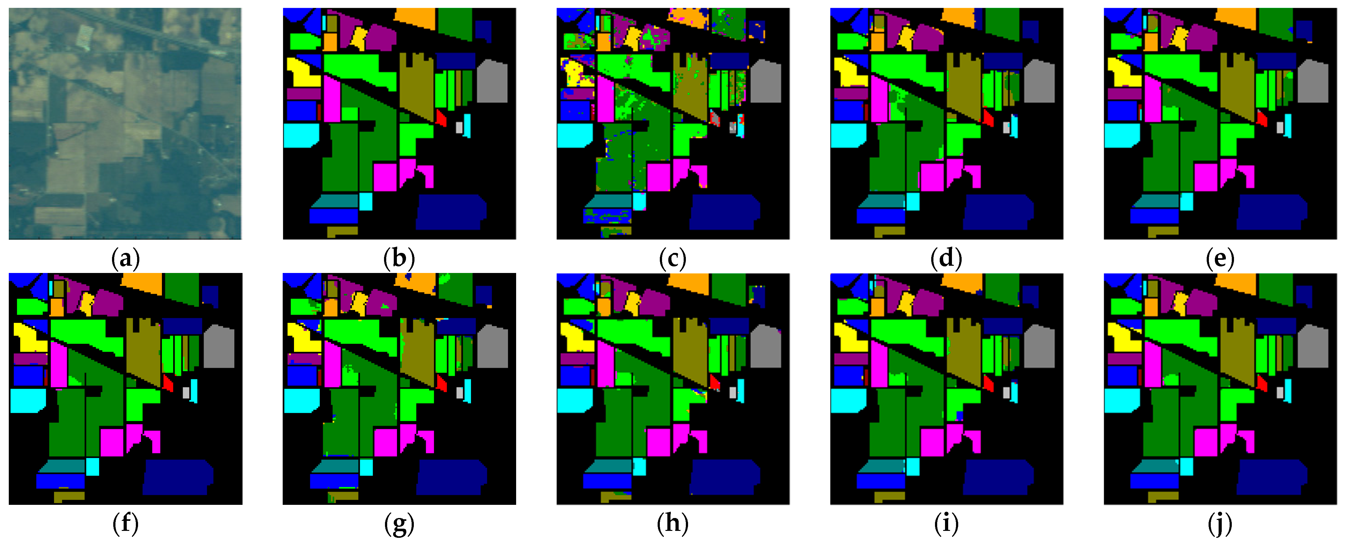
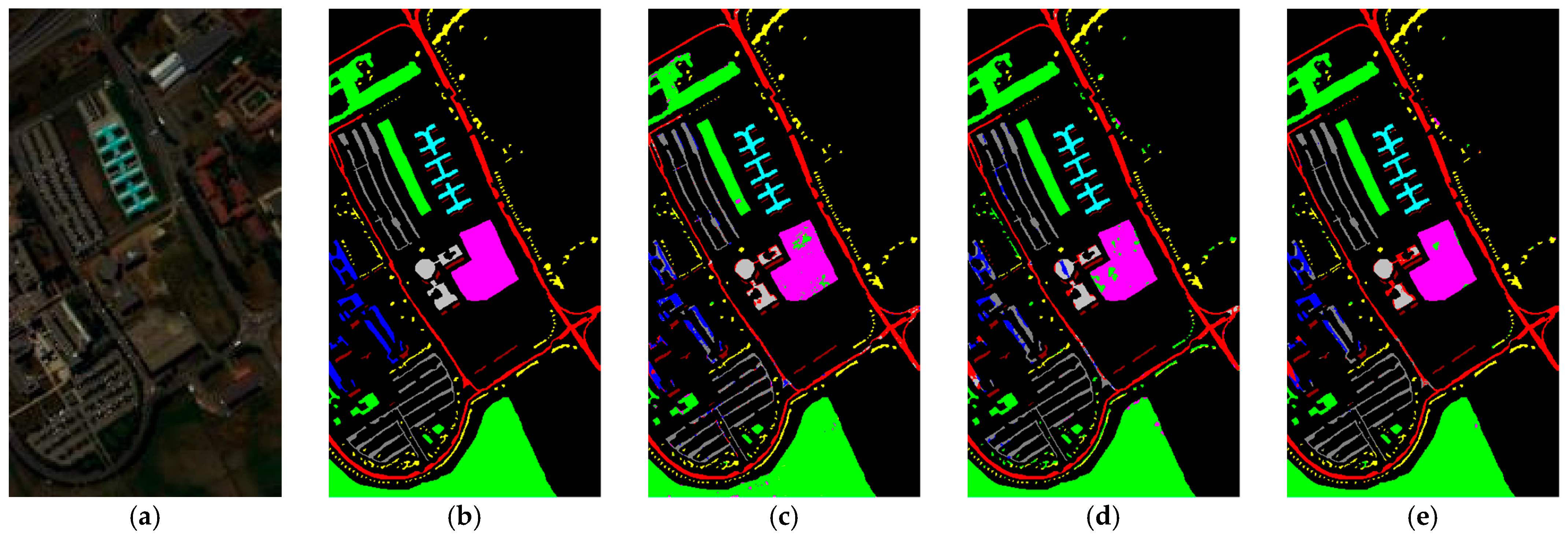
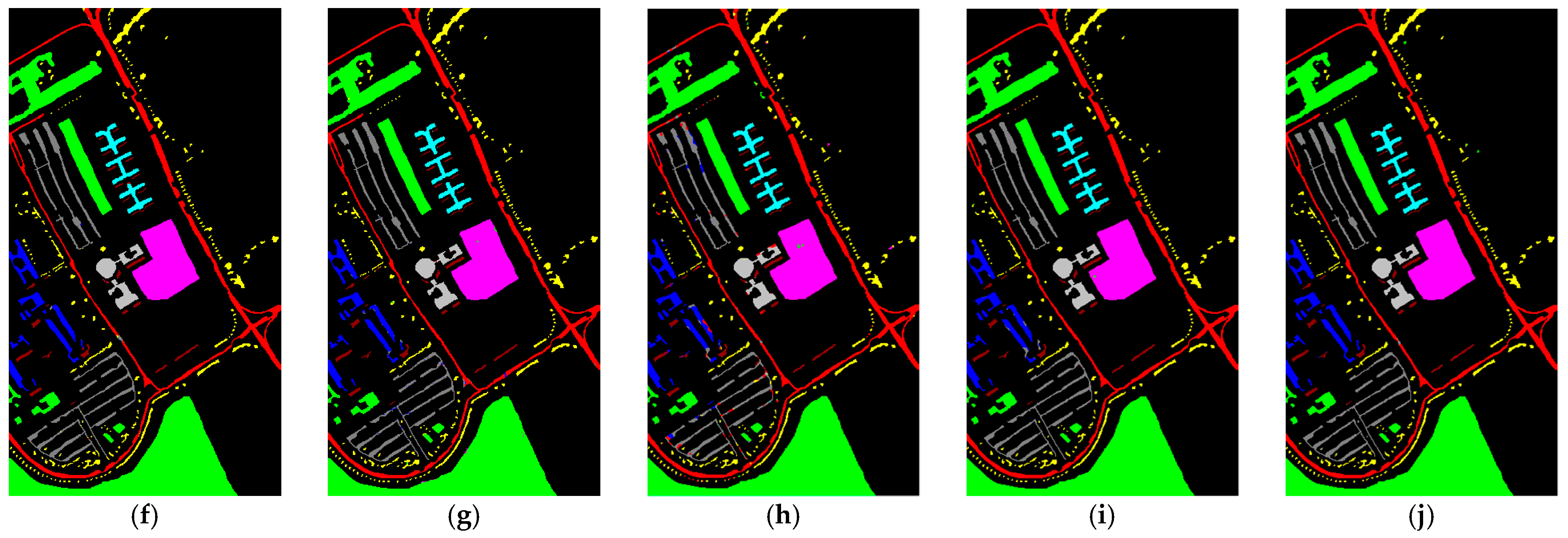
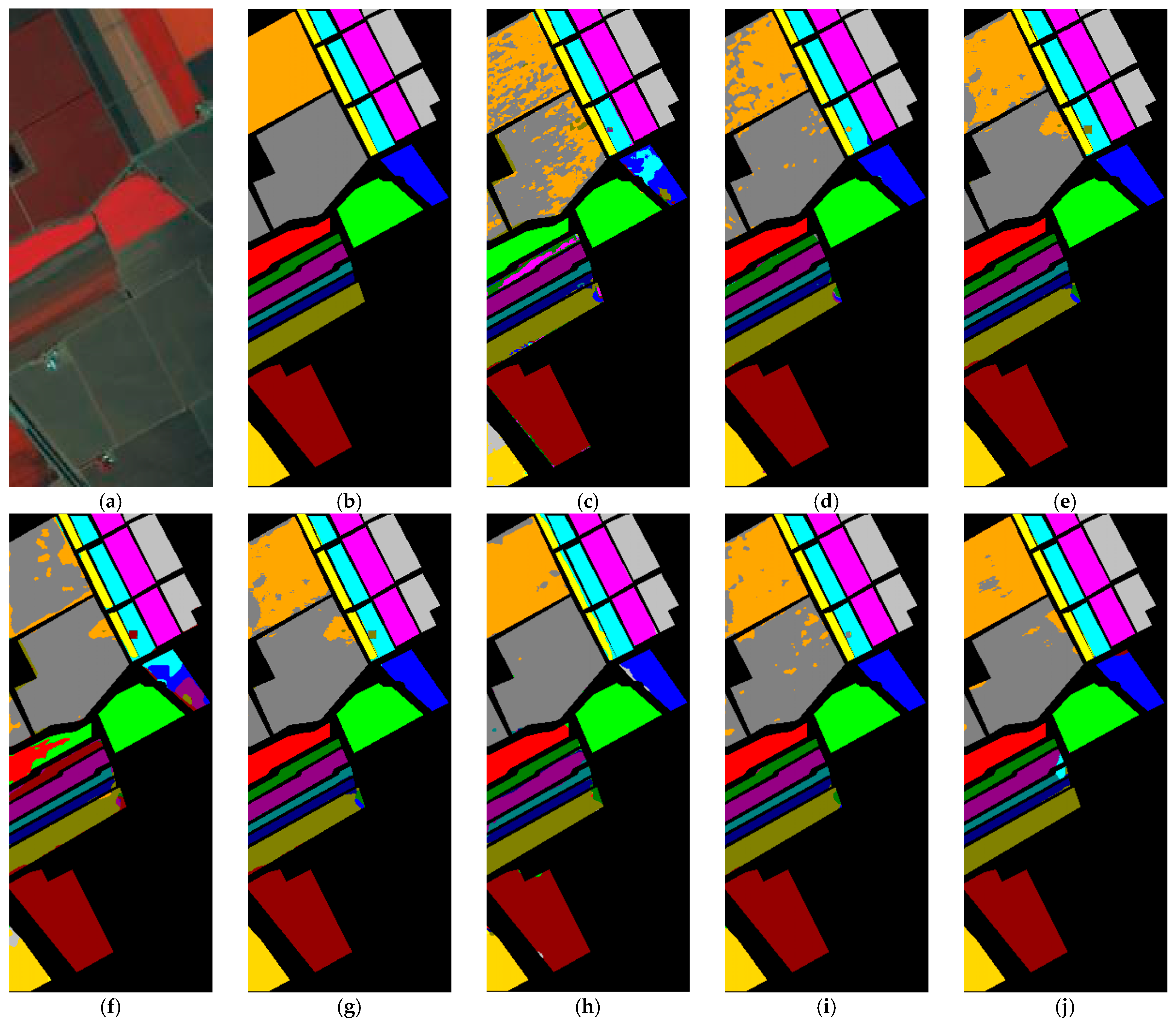
5.2. Classification Results

Compared to other methods, the proposed LVGG model achieved the highest OA and Kappa on three benchmark datasets. The classification plots are shown in Figure 2, Figure 3 and Figure 4, respectively, while Table 4, Table 5 and Table 6 display the algorithms’ classification accuracy regarding the three datasets in detail.

5.2.1. IP

Table 4 shows the classification performance of different models on the IP dataset. Among the compared methods, SSRN, HybridSN, DBDA, and FDSSC employ relatively complex CNN-based frameworks, incorporating elements such as 3D CNN, residual connections, and MLP to enhance classification performance. However, these approaches come at the cost of consumed computational time. In contrast, SSFTT, based on a lightweight transformer architecture, offers a shorter training time but exhibits a slight decrease in accuracy compared to other methods.
GAHT adopts a hybrid approach, combining elements of both transformers and CNNs. This hybrid strategy results in shorter training times while improving accuracy. In comparison to other methods, compared to FDSSC, SSFTT, and GAHT, our LVGG improved 0.22%, 1.06%, and 0.58% in OA and 0.04%, 1.15%, and 0.60% in Kappa, respectively. However, it did show a slightly increased overall training time compared to SSFTT.

5.2.2. PU

For the PU dataset, because we chose a training set percentage of 5%, the training data volume was relatively large. As a result, all methods yielded good results. Among these methods, GAHT and FDSSC were two models that performed well, in addition to our method. The accuracy of Class 3, Class 8, and Class 9 significantly impacted the overall OA. While our method did not perform well in classifying Class 7, it did achieve the highest accuracy in most other classes. Furthermore, the transformer-based SSFTT did not perform as well as the hybrid model GAHT, which combines transformers and CNN. This suggests that convolutional methods still performed effectively on the PU dataset. However, our method still achieved the best OA, AA, and Kappa results while also being the fastest in terms of execution time.

5.2.3. SA

For the SA dataset, we selected only 1% of the data as the training set, which led to lower classification accuracy for the SSFTT method. The low accuracy of SSFTT in classifying Class 8 and Class 15 may be due to the limited number of samples that the transformer learned, coupled with the similarity of features. When dealing with a limited number of HSI samples, there are limitations associated with transformer-based methods; possibly, these methods require a larger amount of data to learn effectively due to weaker inductive biases. In contrast, CNN-based methods tend to perform better under these conditions, and our approach outperformed all others. This could be attributed to the use of a larger patch size, allowing for a broader learning scope that works well with small datasets.

5.3. Ablation Studies

We analyzed the proposed LVGG framework by transitioning from the VGG block to the lightweight-VGG block, and conducted experiments on the IP dataset with the corresponding results summarized in Table 7. First, the activation function of the FC layers was modified from ReLU to SELU, as SELU has self-normalizing properties and performs well in FC layers. Using SELU as the activation function for FC layers improved performance compared to the basic VGG structure.
We also improved the activation function for regular convolutions. While VGG uses ReLU as the activation function, we introduced DyReLU as an alternative to enhance the non-linearity of shallow networks. Using DyReLU as the activation function also resulted in improved accuracy.
Regarding normalization, for the IP dataset, using a large batch size with batch normalization decreased the classification accuracy, while using layer normalization improved the accuracy. Therefore, layer normalization was adopted for normalization in this proposed network.
Activation functions and normalization have an impact on network classification accuracy. Additionally, the expand convolution also contributes to improved accuracy. As we had seven channels after the whitened PCA, using only seven channels for the classification limited the overall convolutional features. Therefore, expanding the convolution before regular the convolution enhances the network’s learning ability and achieves better classification accuracy.

5.4. Parameter Analysis

We analyzed the effect of various parameters on the classification performance of our proposed lightweight-VGG method by conducting experiments using different parameter settings in the same experimental setting as described in Section 5.1.

5.4.1. The Effectiveness of Band Selection

The criteria for determining the number of bands is to minimize it as much as possible while ensuring the accuracy of SVM. As shown in Table 8, the highest accuracy appears when the number of selected bands is 35 on the IP dataset. In addition, when taken as 35, the number of bands and accuracy achieve a certain degree of balance on the other two HSI datasets. Therefore, 35 bands were chosen in this study.

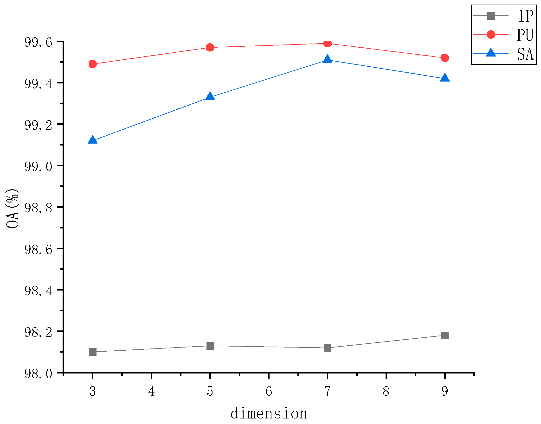
5.4.2. The Effectiveness of PCA Size Selection

We investigated the impact of different PCA dimensions on classification performance, evaluated using overall accuracy. The purpose of PCA dimensionality reduction is to reduce the data’s dimensions, lowering computational cost and noise. By selecting an appropriate PCA dimension, noise or less significant variations can be filtered out. Lower PCA dimensions may filter out important information, while higher PCA dimensions may retain noise. Lower PCA dimensions result in higher data compression but may lead to information loss. Higher PCA dimensions retain more information but increase data dimensionality. Lower PCA dimensions typically enhance computational efficiency, as processing low-dimensional data is faster. However, in our case, we performed PCA after band selection, so setting the PCA dimensions to seven achieved outstanding performances.
As shown in Figure 5, the results with PCA dimensions set to seven were comparable to those retaining more dimensions, indicating that band selection filtered out most of the noise, and that PCA dimensions of seven were sufficient to achieve good performance.

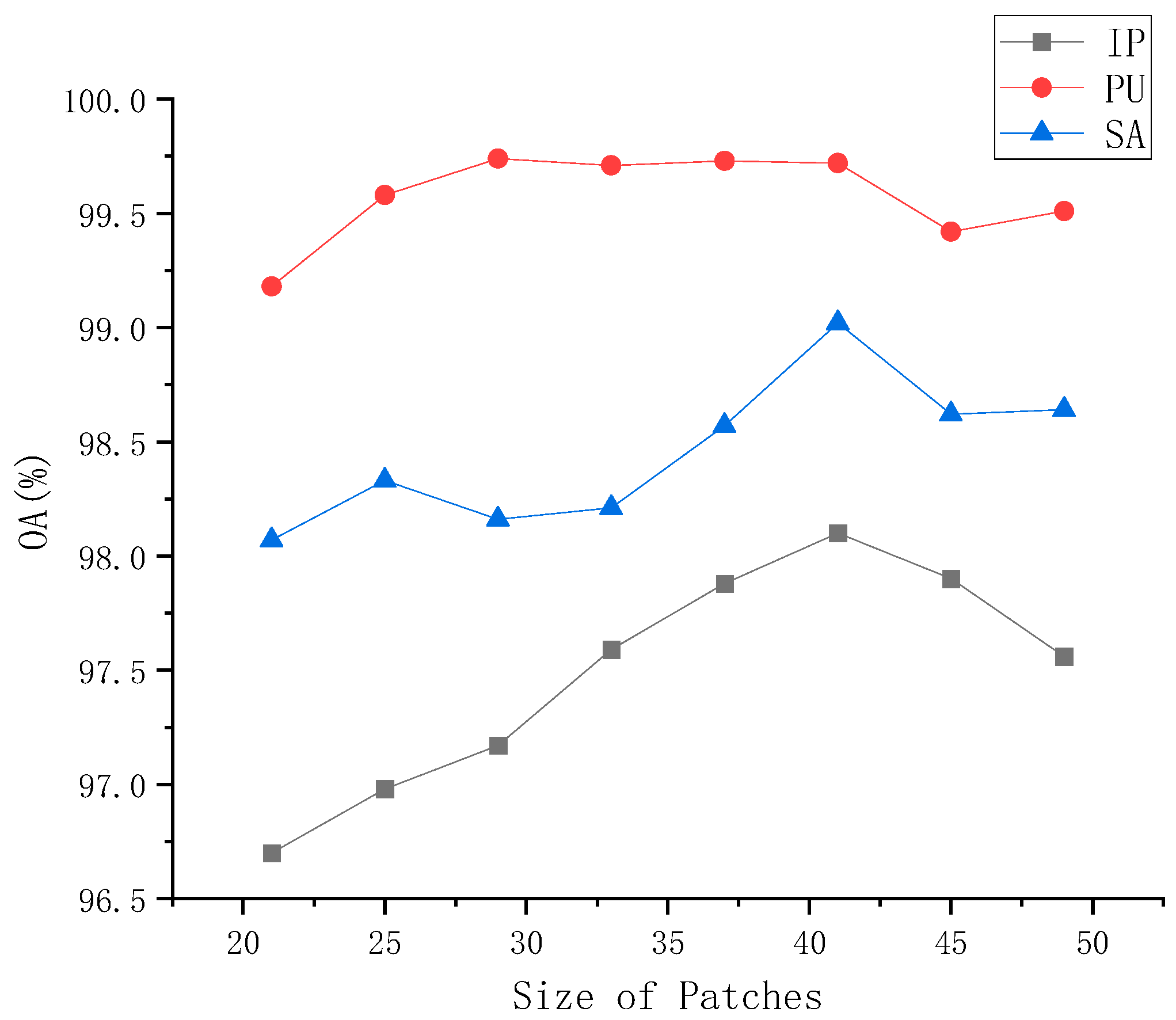
5.4.3. The Effectiveness of Patch Size Selection

We investigated the impact of different patch sizes on classification performance, which we evaluated based on overall accuracy. The patch sizes varied from 21 × 21 to 49 × 49, as shown in Figure 6. As the patch size increased, performance initially improved and then started to decline. When the patch size was set to 41 × 41, we obtained the best performance for the IP, PU, and SA datasets, with OAs of 98.10%, 99.72%, and 99.02%, respectively. The performance of the PU dataset remained relatively stable from 21 × 21 to 49 × 49, possibly due to the high training rate of the PU dataset. However, the IP and SA datasets showed variations in performance. This may be attributed to the use of max-pooling in our method, where smaller image patches did not have sufficient representation, and overly large patches could make the overall structure too complex. Therefore, we chose a patch size of 41 × 41.

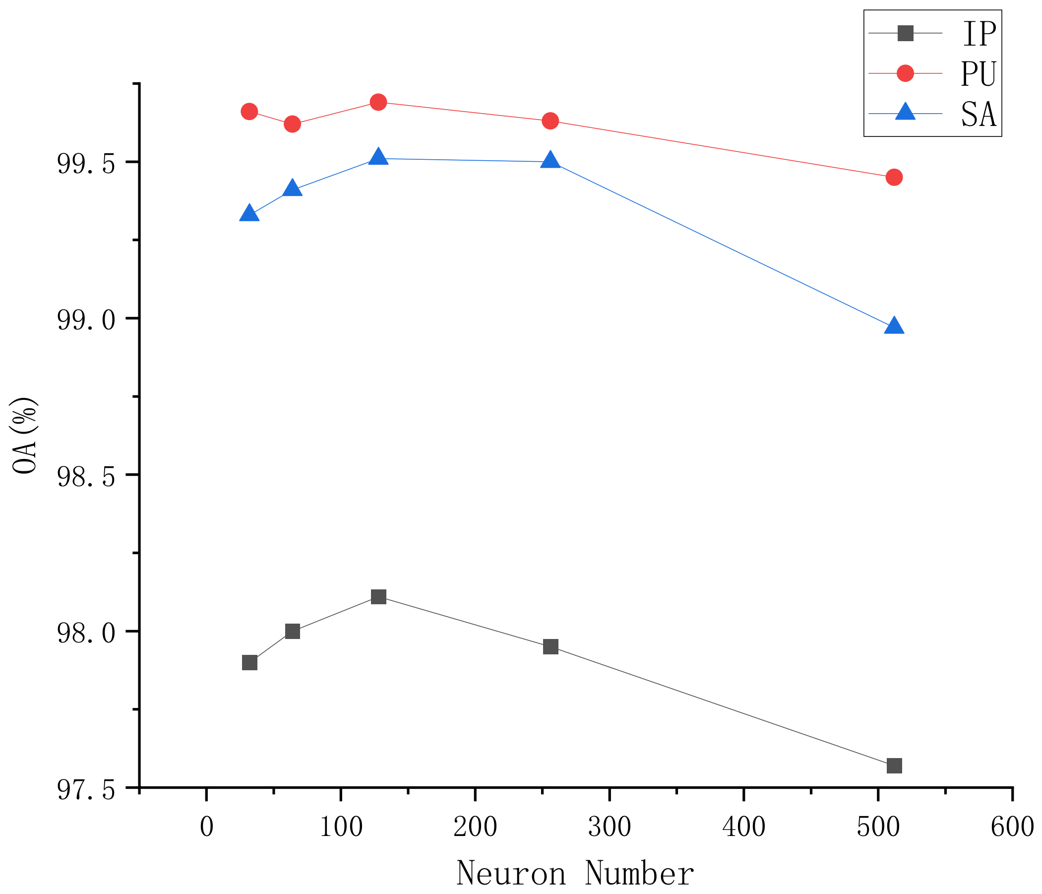
5.4.4. The Effectiveness of Neuron Number in the FC Layer

We investigated the impact of different neuron numbers in the FC layer on classification performance, evaluating based on overall accuracy. Neuron numbers ranged from 32 to 512, as shown in Figure 7. Performance improved with an increase in neurons but began to decline thereafter. On all three datasets, the best performance was generally achieved with 128 neurons, although 64 neurons also showed good results in the SA and PU datasets.

5.5. Computational Efficiency

We also verified computational efficiency by observing the performance of these methods in terms of execution time, number of parameters, and the number of floating-point operations (FLOPs) on three HSI datasets. The statistical results are shown in Table 9.
SSRN is a combination of 3D CNN with a ResNet structure short-circuit.
HybridSN is a network that combines 3D CNN and 2D CNN, resulting in shorter execution times. Because it uses PCA for dimensionality reduction, followed by two rounds of 3D convolution for feature extraction, and because it uses a 2D convolutional network, it results in shorter execution times compared to SSRN.
SSFTT is the fastest model in terms of execution time because it consists of only one layer of 3D CNN and one layer of 2D CNN, followed by the tokenization of features through the transformer. Due to the limited data, the transformer learns quickly. The model has the shortest training time and the least number of parameters. However, the overall accuracy is moderate.
GAHT is a method that combines transformers with CNN, so the overall execution time is similar as well. Although it has the lowest FLOPs, its execution time is not very short due to the involvement of group convolutions.
FDSSC is the most time-consuming CNN network because it involves reconstruction and feature extraction using complex 3D CNN. The high time complexity of 3D CNN results in the longest overall execution time.
DBDA employs dense 3D CNN for learning, much like FDSSC. However, it does not have the reconstruction step that FDSSC has, which significantly reduces its execution time.
In comparison to these methods, our proposed LVGG method has a short execution time because it only utilizes 1 × 1 and 3 × 3 2D convolutions. Its FLOPs are relatively low, but due to a relatively larger number of parameters compared to transformer methods, its runtime is somewhat longer than those of transformer-based approaches.

6. Conclusions

This study proposes a lightweight-VGG approach to improve HSI classification speed and accuracy. In this context, we introduce a method that performs PCA after selecting bands for classification. Most existing works either directly use raw images or apply PCA with a large number of retained dimensions, which can introduce noise and be sensitive to random seeds. Additionally, many transformer-based classification methods involve complex and computationally expensive operations, yet they do not achieve high accuracy in HSI classification. In contrast, our proposed LVGG approach reduces the number of parameters in the fully connected layers, resulting in a faster processing speed while maintaining high classification accuracy.
By performing PCA on the data after selecting the bands, and then conducting network classification, our proposed method provides improved stability and speed. Moreover, its smaller parameter size allows for faster processing, making it suitable for deployment on lightweight devices. Quantitative experiments using three HSI datasets showed that our LVGG approach outperformed existing methods in both performance and speed.

Author Contributions

Methodology, software and writing—original draft preparation, X.F. and S.W.; investigation and data curation, J.M. and G.W.; modification and editing, L.S. All authors have read and agreed to the published version of the manuscript.

Funding

This research was funded by the National Natural Science Foundation of China (62006072, 62106067), the Key Technologies Research and Development Program of Henan Province (222102210108), the Ministry of Education Key Laboratory Open Funded Project for Grain Information Processing and Control (KFJJ2022013), the Natural Science Project of Zhengzhou Science and Technology Bureau (21ZZXTCX21), the Innovative Funds Plan of Henan University of Technology (2022ZKCJ11), and the Cultivation Programme for Young Backbone Teachers in Henan University of Technology.

Data Availability Statement

The data presented in this study are available in the article.

Acknowledgments

The authors would like to thank the editors and reviewers for their advice.

Conflicts of Interest

The authors declare no conflicts of interest.

Abbreviations

The abbreviations for all key terms in this paper are explained below:
HSIHyperspectral Image
SVMSupport Vector Machine
CNNsConvolutional Neural Networks
MLPMulti-Layer Perceptron
FCFully Connected
LNLayer Normalization
BNBatch Normalization
VGGVisual Geometry Group
SELUScaled Exponential Linear Unit
ReLURectified Linear Unit
SSFTT Spectral–Spatial Feature Tokenization Transformer
SSRNSpectral–spatial Residual Network
HybridSNHybrid Spectral–spatial Network
GAHT Group-Aware Transformer
DBDADouble-Branch-Dual-Attention-Mechanism-Network
FDSSCA Fast Dense Spectral–spatial Convolution Network
IPIndian Pines
PUPavia University
SASalinas
AA Average Accuracy
OAOverall Accuracy
KappaKappa coefficient
FLOPsFloating-Point Operations

References

  1. Fan, J.; Chen, T.; Lu, S. Superpixel guided deep-sparse-representation learning for hyperspectral image classification. IEEE Trans. Circuits Syst. Video Technol. 2017, 28, 3163–3173. [Google Scholar] [CrossRef]
  2. Li, M.; Liu, Y.; Xue, G.; Huang, Y.; Yang, G. Exploring the relationship between center and neighborhoods: Central vector oriented self-similarity network for hyperspectral image classification. IEEE Trans. Circuits Syst. Video Technol. 2022, 33, 1979–1993. [Google Scholar] [CrossRef]
  3. Yu, Y.; Fu, L.; Cheng, Y.; Ye, Q. Multi-view distance metric learning via independent and shared feature subspace with applications to face and forest fire recognition, and remote sensing classification. Knowl. Based Syst. 2022, 243, 108350. [Google Scholar] [CrossRef]
  4. Mok, T.C.; Chung, A. Fast symmetric diffeomorphic image registration with convolutional neural networks. In Proceedings of the IEEE/CVF Conference on Computer Vision and Pattern Recognition, Seattle, WA, USA, 13–19 June 2020; pp. 4644–4653. [Google Scholar]
  5. Stuart, M.B.; McGonigle, A.J.; Willmott, J.R. Hyperspectral imaging in environmental monitoring: A review of recent developments and technological advances in compact field deployable systems. Sensors 2019, 19, 3071. [Google Scholar] [CrossRef] [PubMed]
  6. Alamús, R.; Bará, S.; Corbera, J.; Escofet, J.; Palà, V.; Pipia, L.; Tardà, A. Ground-based hyperspectral analysis of the urban nightscape. ISPRS J. Photogramm. Remote Sens. 2017, 124, 16–26. [Google Scholar] [CrossRef]
  7. Sun, Z.; Leng, X.; Lei, Y.; Xiong, B.; Ji, K.; Kuang, G. BiFA-YOLO: A novel YOLO-based method for arbitrary-oriented ship detection in high-resolution SAR images. Remote Sens. 2021, 13, 4209. [Google Scholar] [CrossRef]
  8. Bandos, T.V.; Bruzzone, L.; Camps-Valls, G. Classification of hyperspectral images with regularized linear discriminant analysis. IEEE Trans. Geosci. Remote Sens. 2009, 47, 862–873. [Google Scholar] [CrossRef]
  9. Ghamisi, P.; Yokoya, N.; Li, J.; Liao, W.; Liu, S.; Plaza, J.; Rasti, B.; Plaza, A. Advances in hyperspectral image and signal processing: A comprehensive overview of the state of the art. IEEE Geosci. Remote Sens. Mag. 2017, 5, 37–78. [Google Scholar] [CrossRef]
  10. Fauvel, M.; Benediktsson, J.A.; Chanussot, J.; Sveinsson, J.R. Spectral and spatial classification of hyperspectral data using SVMs and morphological profiles. IEEE Trans. Geosci. Remote Sens. 2008, 46, 3804–3814. [Google Scholar] [CrossRef]
  11. Hong, D.; Wu, X.; Ghamisi, P.; Chanussot, J.; Yokoya, N.; Zhu, X.X. Invariant attribute profiles: A spatial-frequency joint feature extractor for hyperspectral image classification. IEEE Trans. Geosci. Remote Sens. 2020, 58, 3791–3808. [Google Scholar] [CrossRef]
  12. Sun, Z.; Dai, M.; Leng, X.; Lei, Y.; Xiong, B.; Ji, K.; Kuang, G. An anchor-free detection method for ship targets in high-resolution SAR images. IEEE J. Sel. Top. Appl. Earth Obs. Remote Sens. 2021, 14, 7799–7816. [Google Scholar] [CrossRef]
  13. Hong, D.; Yokoya, N.; Chanussot, J.; Zhu, X.X. An augmented linear mixing model to address spectral variability for hyperspectral unmixing. IEEE Trans. Image Process. 2018, 28, 1923–1938. [Google Scholar] [CrossRef] [PubMed]
  14. Shahshahani, B.M.; Landgrebe, D.A. The effect of unlabeled samples in reducing the small sample size problem and mitigating the Hughes phenomenon. IEEE Trans. Geosci. Remote Sens. 1994, 32, 1087–1095. [Google Scholar] [CrossRef]
  15. Dash, M.; Liu, H. Feature selection for classification. Intell. Data Anal. 1997, 1, 131–156. [Google Scholar] [CrossRef]
  16. Guyon, I.; Elisseeff, A. An introduction to variable and feature selection. J. Mach. Learn. Res. 2003, 3, 1157–1182. [Google Scholar]
  17. Martinez, A.M.; Kak, A.C. Pca versus lda. IEEE Trans. Pattern Anal. Mach. Intell. 2001, 23, 228–233. [Google Scholar] [CrossRef]
  18. Draper, B.A.; Baek, K.; Bartlett, M.S.; Beveridge, J.R. Recognizing faces with PCA and ICA. Comput. Vis. Image Underst. 2003, 91, 115–137. [Google Scholar] [CrossRef]
  19. Cortes, C.; Vapnik, V. Support-vector networks. Mach. Learn. 1995, 20, 273–297. [Google Scholar] [CrossRef]
  20. Breiman, L. Random forests. Mach. Learn. 2001, 45, 5–32. [Google Scholar] [CrossRef]
  21. Yang, X.; Ye, Y.; Li, X.; Lau, R.Y.; Zhang, X.; Huang, X. Hyperspectral image classification with deep learning models. IEEE Trans. Geosci. Remote Sens. 2018, 56, 5408–5423. [Google Scholar] [CrossRef]
  22. Wang, W.; Dou, S.; Jiang, Z.; Sun, L. A fast dense spectral–spatial convolution network framework for hyperspectral images classification. Remote Sens. 2018, 10, 1068. [Google Scholar] [CrossRef]
  23. Roy, S.K.; Krishna, G.; Dubey, S.R.; Chaudhuri, B.B. HybridSN: Exploring 3-D–2-D CNN feature hierarchy for hyperspectral image classification. IEEE Geosci. Remote Sens. Lett. 2019, 17, 277–281. [Google Scholar] [CrossRef]
  24. Li, R.; Zheng, S.; Duan, C.; Yang, Y.; Wang, X. Classification of hyperspectral image based on double-branch dual-attention mechanism network. Remote Sens. 2020, 12, 582. [Google Scholar] [CrossRef]
  25. Chen, Y.; Jiang, H.; Li, C.; Jia, X.; Ghamisi, P. Deep feature extraction and classification of hyperspectral images based on convolutional neural networks. IEEE Trans. Geosci. Remote Sens. 2016, 54, 6232–6251. [Google Scholar] [CrossRef]
  26. Hong, D.; Han, Z.; Yao, J.; Gao, L.; Zhang, B.; Plaza, A.; Chanussot, J. SpectralFormer: Rethinking hyperspectral image classification with transformers. IEEE Trans. Geosci. Remote Sens. 2021, 60, 5518615. [Google Scholar] [CrossRef]
  27. Mei, S.; Song, C.; Ma, M.; Xu, F. Hyperspectral image classification using group-aware hierarchical transformer. IEEE Trans. Geosci. Remote Sens. 2022, 60, 5539014. [Google Scholar] [CrossRef]
  28. Sun, L.; Zhao, G.; Zheng, Y.; Wu, Z. Spectral–spatial feature tokenization transformer for hyperspectral image classification. IEEE Trans. Geosci. Remote Sens. 2022, 60, 5522214. [Google Scholar] [CrossRef]
  29. Zhao, G.; Ye, Q.; Sun, L.; Wu, Z.; Pan, C.; Jeon, B. Joint classification of hyperspectral and lidar data using a hierarchical cnn and transformer. IEEE Trans. Geosci. Remote Sens. 2022, 61, 5500716. [Google Scholar] [CrossRef]
  30. Zhang, Z.; Ma, Q.; Zhou, H.; Gong, N. Nested Transformers for Hyperspectral Image Classification. J. Sens. 2022, 2022, 6785966. [Google Scholar] [CrossRef]
  31. Zhang, X.; Su, Y.; Gao, L.; Bruzzone, L.; Gu, X.; Tian, Q. A Lightweight Transformer Network for Hyperspectral Image Classification. IEEE Trans. Geosci. Remote Sens. 2023, 61, 5517617. [Google Scholar] [CrossRef]
  32. Ye, Q.; Huang, P.; Zhang, Z.; Zheng, Y.; Fu, L.; Yang, W. Multiview Learning With Robust Double-Sided Twin SVM. IEEE Trans. Cybern. 2022, 52, 12745–12758. [Google Scholar] [CrossRef]
  33. Simonyan, K.; Zisserman, A. Very deep convolutional networks for large-scale image recognition. arXiv 2014, arXiv:1409.1556. [Google Scholar]
  34. Mei, S.; Ji, J.; Geng, Y.; Zhang, Z.; Li, X.; Du, Q. Unsupervised spatial–spectral feature learning by 3D convolutional autoencoder for hyperspectral classification. IEEE Trans. Geosci. Remote Sens. 2019, 57, 6808–6820. [Google Scholar] [CrossRef]
  35. Hang, R.; Liu, Q.; Hong, D.; Ghamisi, P. Cascaded recurrent neural networks for hyperspectral image classification. IEEE Trans. Geosci. Remote Sens. 2019, 57, 5384–5394. [Google Scholar] [CrossRef]
  36. Paoletti, M.E.; Haut, J.M.; Plaza, J.; Plaza, A. A new deep convolutional neural network for fast hyperspectral image classification. ISPRS J. Photogramm. Remote Sens. 2018, 145, 120–147. [Google Scholar] [CrossRef]
  37. Yu, S.; Jia, S.; Xu, C. Convolutional neural networks for hyperspectral image classification. Neurocomputing 2017, 219, 88–98. [Google Scholar] [CrossRef]
  38. Li, S.; Song, W.; Fang, L.; Chen, Y.; Ghamisi, P.; Benediktsson, J.A. Deep learning for hyperspectral image classification: An overview. IEEE Trans. Geosci. Remote Sens. 2019, 57, 6690–6709. [Google Scholar] [CrossRef]
  39. Li, X.; Ding, M.; Pižurica, A. Deep feature fusion via two-stream convolutional neural network for hyperspectral image classification. IEEE Trans. Geosci. Remote Sens. 2019, 58, 2615–2629. [Google Scholar] [CrossRef]
  40. Hao, S.; Wang, W.; Ye, Y.; Nie, T.; Bruzzone, L. Two-stream deep architecture for hyperspectral image classification. IEEE Trans. Geosci. Remote Sens. 2017, 56, 2349–2361. [Google Scholar] [CrossRef]
  41. Li, Y.; Zhang, H.; Shen, Q. Spectral–spatial classification of hyperspectral imagery with 3D convolutional neural network. Remote Sens. 2017, 9, 67. [Google Scholar] [CrossRef]
  42. Zhong, Z.; Li, J.; Luo, Z.; Chapman, M. Spectral–spatial residual network for hyperspectral image classification: A 3-D deep learning framework. IEEE Trans. Geosci. Remote Sens. 2017, 56, 847–858. [Google Scholar] [CrossRef]
  43. Fu, L.; Zhang, D.; Ye, Q. Recurrent thrifty attention network for remote sensing scene recognition. IEEE Trans. Geosci. Remote Sens. 2020, 59, 8257–8268. [Google Scholar] [CrossRef]
  44. Sun, L.; Fang, Y.; Chen, Y.; Huang, W.; Wu, Z.; Jeon, B. Multi-structure KELM with attention fusion strategy for hyperspectral image classification. IEEE Trans. Geosci. Remote Sens. 2022, 60, 5539217. [Google Scholar] [CrossRef]
  45. Hu, J.; Shen, L.; Sun, G. Squeeze-and-excitation networks. In Proceedings of the IEEE Conference on Computer Vision and Pattern Recognition, Salt Lake City, UT, USA, 18–23 June 2018; pp. 7132–7141. [Google Scholar]
  46. Woo, S.; Park, J.; Lee, J.-Y.; Kweon, I.S. Cbam: Convolutional block attention module. In Proceedings of the European Conference on Computer Vision (ECCV), Munich, Germany, 8–14 September 2018; pp. 3–19. [Google Scholar]
  47. Zhu, M.; Jiao, L.; Liu, F.; Yang, S.; Wang, J. Residual spectral–spatial attention network for hyperspectral image classification. IEEE Trans. Geosci. Remote Sens. 2020, 59, 449–462. [Google Scholar] [CrossRef]
  48. He, X.; Chen, Y.; Lin, Z. Spatial-spectral transformer for hyperspectral image classification. Remote Sens. 2021, 13, 498. [Google Scholar] [CrossRef]
  49. Van Der Maaten, L.; Postma, E.O.; van den Herik, H.J. Dimensionality reduction: A comparative review. J. Mach. Learn. Res. 2009, 10, 13. [Google Scholar]
  50. Fu, L.; Li, Z.; Ye, Q.; Yin, H.; Liu, Q.; Chen, X.; Fan, X.; Yang, W.; Yang, G. Learning Robust Discriminant Subspace Based on Joint L2,p- and L2,s-Norm Distance Metrics. IEEE Trans. Neural Netw. Learn. Syst. 2022, 33, 130–144. [Google Scholar] [CrossRef] [PubMed]
  51. Ye, Q.; Li, Z.; Fu, L.; Zhang, Z.; Yang, W.; Yang, G. Nonpeaked discriminant analysis for data representation. IEEE Trans. Neural Netw. Learn. Syst. 2019, 30, 3818–3832. [Google Scholar] [CrossRef] [PubMed]
  52. Li, W.; Prasad, S.; Fowler, J.E.; Bruce, L.M. Locality-preserving dimensionality reduction and classification for hyperspectral image analysis. IEEE Trans. Geosci. Remote Sens. 2011, 50, 1185–1198. [Google Scholar] [CrossRef]
  53. Wang, Q.; Li, Q.; Li, X. A fast neighborhood grouping method for hyperspectral band selection. IEEE Trans. Geosci. Remote Sens. 2020, 59, 5028–5039. [Google Scholar] [CrossRef]
  54. Liu, Z.; Mao, H.; Wu, C.-Y.; Feichtenhofer, C.; Darrell, T.; Xie, S. A convnet for the 2020s. In Proceedings of the IEEE/CVF Conference on Computer Vision and Pattern Recognition, New Orleans, LA, USA, 18–24 June 2022; pp. 11976–11986. [Google Scholar]
  55. Howard, A.G.; Zhu, M.; Chen, B.; Kalenichenko, D.; Wang, W.; Weyand, T.; Andreetto, M.; Adam, H. Mobilenets: Efficient convolutional neural networks for mobile vision applications. arXiv 2017, arXiv:1704.04861. [Google Scholar]
  56. Klambauer, G.; Unterthiner, T.; Mayr, A.; Hochreiter, S. Self-normalizing neural networks. Adv. Neural Inf. Process. Syst. 2017, 30, 971–980. [Google Scholar]
Figure 1. Overview of the proposed LVGG framework, which consists of two main components: a strategy for removing redundant data and a strategy for designing a lightweight VGG-based network structure.
Remotesensing 16 00259 g001
Figure 2. Classification maps of different methods for the IP dataset. (a) False-color image. (b) Ground truth image. (c) 3D CNN. (d) SSRN. (e) HybridSN. (f) SSFTT. (g) GAHT. (h) DBDA. (i) FDSSC. (j) LVGG.
Remotesensing 16 00259 g002
Figure 3. Classification maps of different methods for the PU dataset. (a) False-color image. (b) Ground truth image. (c) 3D CNN. (d) SSRN. (e) HybridSN. (f) SSFTT. (g) GAHT. (h) DBDA. (i) FDSSC. (j) LVGG.
Remotesensing 16 00259 g003aRemotesensing 16 00259 g003b
Figure 4. Classification maps of different methods for the SA dataset. (a) False-color image. (b) Ground truth image. (c) 3D CNN. (d) SSRN. (e) HybridSN. (f) SSFTT. (g) GAHT. (h) DBDA. (i) FDSSC. (j) LVGG.
Remotesensing 16 00259 g004
Figure 5. The three HSI datasets with distinct PCA dimensions for OA.
Remotesensing 16 00259 g005
Figure 6. The three HSI datasets with distinct patch sizes for OA.
Remotesensing 16 00259 g006
Figure 7. The three HSI datasets with distinct neuron numbers for OA.
Remotesensing 16 00259 g007
Table 1. The class names and the training, validation and test sample numbers in IP.
ClassLand Cover TypeTrain.Val.Test.
1Alfalfa5536
2Corn-No till1431431142
3Corn-Min till8383664
4Corn2424189
5Grass-Pasture4848387
6Grass-Trees7373584
7Grass-Pasture-Mowed3322
8Hay-Windrowed4848382
9Oats2216
10Soybean-No till9797778
11Soybean-Min till2452451965
12Soybean-Clean5959475
13Wheat2020165
14Woods1261261013
15Buildings-Grass-Trees-Drives3939308
16Stone-Steel-Towers9975
Total102410248201
Table 2. The class names and the training, validation and test sample numbers in PU.
ClassLand Cover TypeTrain.Val.Test.
1Asphalt3323325967
2Meadows93293216,785
3Gravel1051051889
4Trees1531532758
5Painted Metal Sheets67671211
6Bare Soil2512514527
7Bitumen67671196
8Self-Blocking Bricks1841843314
9Shadows4747853
Total2138213838,500
Table 3. The class names and the training, validation and test sample numbers in SA.
ClassLand Cover TypeTrain.Val.Test.
1Brocoli-green-weeds-120201969
2Brocoli-green-weeds-237373652
3Fallow20201936
4Fallow-rough-plow14141366
5Fallow-smooth27272624
6Stubble39393881
7Celery36363507
8Grapes-untrained11311311,045
9Soil-vinyard-develop62626079
10Corn-senesced-green-weeds33333212
11Lettuce-romaine-4wk11111046
12Lettuce-romaine-5wk19191889
13Lettuce-romaine-6wk99898
14Lettuce-romaine-7wk11111048
15Vinyard-untrained72727124
16Vinyard-vertical-trellis18181771
Total54154153,047
Table 4. The classification accuracy of the IP dataset.
Class3D CNNSSRNHybridSNSSFTTGAHTDBDAFDSSCLVGG
158.54 ± 3.1594.14 ± 2.1692.68 ± 1.7395.12 ± 3.5197.56 ± 1.2398.30 ± 1.66100 ± 097.62 ± 1.71
276.19 ± 1.6997.84 ± 0.8696.62 ± 0.6697.67 ± 1.1398.05 ± 1.2597.95 ± 1.2999.73  ± 0.2697.74 ± 0.79
377.64 ± 2.3097.54 ± 1.7998.41 ± 0.5498.87 ± 0.3598.66 ± 0.8899.40  ± 0.4198.89 ± 0.8098.28 ± 0.73
452.11 ± 4.4890.70 ± 3.1098.97 ± 1.1791.55 ± 4.7395.31 ± 3.26100 ± 0100 ± 099.52 ± 0.73
593.56 ± 0.8897.75 ± 1.3297.70 ± 1.2696.32 ± 1.5295.17 ± 2.6997.84 ± 1.5798.83 ± 0.6799.10  ± 1.01
698.17 ± 0.7299.24 ± 0.5599.69 ± 0.1199.54 ± 0.4599.85  ± 0.1498.82 ± 1.5299.65 ± 0.3398.70 ± 0.20
736.00 ± 5.1281.60 ± 4.0198.85 ± 0.38100  ± 0100  ± 092.91 ± 9.8695.23 ± 3.6299.16 ± 1.67
898.60 ± 1.19100  ± 0100  ± 0100  ± 0100  ± 099.67 ± 0.3198.97 ± 0.40100  ± 0
955.56 ± 2.4574.44 ± 1.0398.38 ± 3.2688.89 ± 3.48100 ± 093.75 ± 3.16100  ± 094.74 ± 0.96
1082.86 ± 3.0294.77 ± 3.0698.08 ± 0.8197.71 ± 1.4294.29 ± 2.3098.47 ± 1.7795.3 ± 2.2199.66 ± 0.40
1190.45 ± 1.3398.87 ± 0.9097.47 ± 1.3398.69 ± 1.2899.37 ± 0.4898.39 ± 0.9199.53  ± 0.4496.97 ± 0.64
1262.55 ± 1.1797.83 ± 2.1398.85 ± 1.0298.13 ± 1.7796.63 ± 0.9799.36 ± 0.2698.73 ± 0.7299.40 ± 0.51
1388.65 ± 3.5899.24 ± 0.3299.82 ± 0.2497.28 ± 2.6499.68 ± 0.4096.36 ± 1.46100  ± 0100  ± 0
1499.39 ± 0.6099.18 ± 0.7799.13 ± 0.9299.91  ± 0.0797.89 ± 2.1699.40 ± 0.4499.02 ± 0.4999.91  ± 0.09
1586.17 ± 2.8593.95 ± 2.38100  ± 098.84 ± 2.4997.12 ± 1.5895.59 ± 2.5996.15 ± 1.3199.14 ± 0.95
1645.24 ± 5.3698.33  ± 1.5591.57 ± 4.0795.54 ± 3.0794.05 ± 3.1393.33 ± 4.1096.05 ± 2.4594.54 ± 5.62
OA (%)85.42 ± 3.7596.88 ± 0.4197.59 ± 0.5697.47 ± 0.3397.95 ± 0.2898.10 ± 0.2198.31 ± 0.1798.53  ± 0.38
AA (%)85.10 ± 2.9897.51 ± 0.5397.27 ± 0.9396.57 ± 0.4897.75 ± 0.5598.35 ± 0.7298.63  ± 0.7297.44 ± 1.03
Kappa × 10083.24 ± 2.3197.23 ± 0.5296.90 ± 0.3797.11 ± 0.4497.66 ± 0.3898.01 ± 0.4198.22 ± 0.6598.26  ± 0.44
The highest values in each row are marked in bold to highlight the performance.
Table 5. The classification accuracy of the PU dataset.
Class3D CNNSSRNHybridSNSSFTTGAHTDBDAFDSSCLVGG
197.02 ± 1.7099.29 ± 0.2498.81 ± 0.7699.33 ± 0.1599.38 ± 0.1599.67 ± 0.2499.76 ± 0.1099.83  ± 0.06
298.82 ± 1.1799.71 ± 0.1999.83 ± 0.1799.92 ± 0.0599.80 ± 0.1099.85 ± 0.1499.80 ± 0.0499.94  ± 0.03
392.98 ± 1.3196.92 ± 3.1592.45 ± 4.9098.29 ± 0.9598.35 ± 0.8599.41 ± 0.7298.95 ± 1.1499.72  ± 0.26
497.53 ± 1.5899.89 ± 0.1198.32 ± 0.8898.49 ± 1.4099.52 ± 0.4098.96 ± 0.6999.92  ± 0.0899.30 ± 0.33
599.06 ± 1.2099.52 ± 0.4999.65 ± 0.2999.53 ± 0.5099.88 ± 0.1299.82 ± 0.1799.91  ± 0.0799.65 ± 0.39
699.10 ± 0.8599.87 ± 0.1699.43 ± 0.5699.21 ± 0.4899.75 ± 0.0599.91 ± 0.0999.90 ± 0.0399.96 ± 0.04
779.10 ± 8.9799.76  ± 0.2699.76± 0.1999.13 ± 1.0199.60 ± 0.3299.44 ± 0.1199.68 ± 0.2299.06 ± 1.27
897.34 ± 1.0297.36 ± 1.6899.52  ± 0.5098.05 ± 0.5798.63 ± 0.2796.13 ± 3.1099.45 ± 0.1699.39 ± 0.59
995.22 ± 2.5599.66 ± 0.2399.82 ± 0.2395.44 ± 2.1799.53 ± 0.1698.89 ± 1.1599.83  ± 0.0599.10 ± 0.22
OA (%)97.88 ± 0.3599.33 ± 0.2999.10 ± 0.4499.21 ± 0.3699.43 ± 0.1599.37 ± 0.4099.55 ± 0.1799.76  ± 0.08
AA (%)95.26 ± 0.2999.16 ± 0.1898.60 ± 0.3298.69 ± 0.4499.37 ± 0.2199.12 ± 0.4999.22 ± 0.2399.56  ± 0.21
Kappa × 10097.19 ± 0.3999.14 ± 0.2298.81 ± 0.7199.15 ± 0.3999.39 ± 0.0899.09 ± 0.5399.18 ± 0.2499.69  ± 0.06
The highest values in each row are marked in bold to highlight the performance.
Table 6. The classification accuracy of the SA dataset.
Class3D CNNSSRNHybridSNSSFTTGAHTDBDAFDSSCLVGG
197.07 ± 1.19100 ± 099.76 ± 0.24100 ± 099.45 ± 1.07100 ± 0100 ± 0100 ± 0
299.86 ± 0.14100 ± 099.97 ± 0.0299.66 ± 0.52100 ± 099.31 ± 0.1199.93 ± 0.05100 ± 0
392.14 ± 2.2098.60 ± 1.0795.81 ± 3.3996.73 ± 1.7195.76 ± 3.8399.67 ± 0.3299.89 ± 0.1199.78 ± 0.19
498.33 ± 0.6298.39 ± 2.2496.05 ± 2.3299.22 ± 0.6198.90 ± 0.5198.03 ± 1.0198.36 ± 0.9295.90 ± 4.13
596.23 ± 0.97100 ± 093.62 ± 3.0796.59 ± 2.6898.88 ± 0.6199.73 ± 0.2699.83 ± 0.0795.96 ± 2.41
699.58 ± 0.4099.98 ± 0.0199.46 ± 0.5399.69 ± 0.37100 ± 0100 ± 0100 ± 098.87 ± 1.33
799.38 ± 0.3199.98 ± 0.0294.59 ± 1.3199.70 ± 0.2199.91 ± 0.0999.96 ± 0.0699.90 ± 0.09100 ± 0
883.96 ± 1.8491.42 ± 5.4596.78 ± 1.7587.59 ± 1.4693.18 ± 2.0489.86 ± 6.4494.53 ± 1.4697.68 ± 3.32
997.89 ± 1.1599.83 ± 0.1698.85 ± 1.2098.91 ± 1.2299.87 ± 0.1099.37 ± 0.6699.86 ± 0.1199.55 ± 0.65
1089.27 ± 1.7198.86 ± 0.6698.60 ± 1.6994.51 ± 1.7196.88 ± 1.1999.30 ± 0.3399.33 ± 0.0998.97 ± 1.19
1183.08 ± 9.2798.39 ± 0.8693.23 ± 1.3196.70 ± 2.2599.06 ± 0.8198.15 ± 1.4398.13 ± 0.9899.70 ± 0.33
1299.06 ± 0.9598.71 ± 1.5597.62 ± 1.9999.88 ± 0.0799.84 ± 0.2399.82 ± 0.1599.75 ± 0.2597.97 ± 3.48
1397.62 ± 2.4999.51 ± 0.5390.57 ± 5.4297.84 ± 2.6699.60 ± 0.3899.86 ± 0.16100 ± 0100 ± 0
1496.36 ± 2.6798.23 ± 0.4794.63 ± 2.0091.80 ± 4.8598.07 ± 2.7598.19 ± 1.5998.48 ± 1.1199.77 ± 0.21
1574.55 ± 6.0893.65 ± 5.8298.50 ± 2.2981.42 ± 3.7790.82 ± 3.4793.17 ± 6.1797.39 ± 1.2799.29 ± 0.62
1691.76 ± 4.1299.82 ± 0.1399.27 ± 0.7297.09 ± 1.5896.87 ± 0.72100 ± 099.26 ± 0.54100 ± 0
OA (%)90.89 ± 0.6196.90 ± 0.6997.16 ± 0.5793.73 ± 0.3996.80 ± 0.3796.44 ± 1.5198.01 ± 0.2498.69 ± 0.70
AA (%)93.51 ± 0.6298.38 ± 0.3096.54 ± 0.6896.08 ± 0.4798.00 ± 0.2498.95 ± 0.2998.54 ± 0.1798.80 ± 0.81
Kappa × 10089.86 ± 0.5796.50 ± 0.7796.84 ± 0.4493.01 ± 0.4496.44 ± 0.3397.79 ± 0.7397.94 ± 0.2798.54 ± 0.65
The highest values in each row are marked in bold to highlight the performance.
Table 7. Ablation analysis of the proposed LVGG on the IP dataset.
ChangesOA (%)
(a) Baseline97.13
(b) Redundant Data Removal97.75
(c) Expand Convolution97.70
(d) DyVGG Block98.03
(e) Multi-Layer Perceptron97.55
(b) + (c) + (d)98.22
(b) + (c) + (e)97.86
(b) + (c) + (d) + (e)98.36
Table 8. Impact of band selection on OA (%) for three datasets.
1520253035404550
IP78.6680.280.8181.2682.8982.782.8782.46
PU89.5290.0993.0293.1793.2693.2993.4193.48
SA91.7191.8592.0792.3392.4592.4192.5092.55
Table 9. Analysis of computing efficiency among different methods on the IP dataset.
Model3D CNNSSRNHybridSNSSFTTGAHTDBDAFDSSCLVGG
Train Time (s)161.0480.9667.4310.7053.36116.01798.7719.95
Test Time (s)6.333.822.850.292.416.166.252.62
Number of Parameters623,281364,1685,122,176148,488972,624382,3261,227,490758,672
GFLOPs1.8591.5391.4960.7500.1531.7651.7220.585
Disclaimer/Publisher’s Note: The statements, opinions and data contained in all publications are solely those of the individual author(s) and contributor(s) and not of MDPI and/or the editor(s). MDPI and/or the editor(s) disclaim responsibility for any injury to people or property resulting from any ideas, methods, instructions or products referred to in the content.

