SGR: An Improved Point-Based Method for Remote Sensing Object Detection via Dual-Domain Alignment Saliency-Guided RepPoints

Abstract

With the advancement of deep neural networks, several methods leveraging convolution neural networks (CNNs) have gained prominence in the field of remote sensing object detection. Acquiring accurate feature representations from feature maps is a critical step in CNN-based object detection methods. Previously, region of interest (RoI)-based methods have been widely used, but of late, deformable convolution network (DCN)-based approaches have started receiving considerable attention. A significant challenge in the use of DCN-based methods is the inefficient distribution patterns of sampling points, stemming from a lack of effective and flexible guidance. To address this, our study introduces Saliency-Guided RepPoints (SGR), an innovative framework designed to enhance feature representation quality in remote sensing object detection. SGR employs a dynamic dual-domain alignment (DDA) training strategy to mitigate potential misalignment issues between spatial and feature domains during the learning process. Furthermore, we propose an interpretable visualization method to assess the alignment between feature representation and classification performance in DCN-based methods, providing theoretical analysis and validation for the effectiveness of sampling points. In this study, we assessed the proposed SGR framework through a series of experiments conducted on four varied and rigorous datasets: DOTA, HRSC2016, DIOR-R, and UCAS-AOD, all of which are widely employed in remote sensing object detection. The outcomes of these experiments substantiate the effectiveness of the SGR framework, underscoring its potential to enhance the accuracy of object detection within remote sensing imagery.

1. Introduction

In the field of remote sensing image interpretation and processing, object detection has become an essential task, and with the advancement of deep neural networks, several methods based on convolution neural networks (CNNs) are becoming prevalent [1,2,3]. Obtaining accurate feature representation of targets from feature maps is a crucial step in accurately predicting targets, especially for targets with arbitrary orientations and complex backgrounds in remote sensing object detection [4,5]. There are two methods that can enhance the quality of the obtained feature representation. In the past, the region of interest (RoI)-based method [6,7] has been primarily used, but now the deformable convolution network (DCN)-based method [8,9,10] is also receiving increasing attention.

The RoI-based methods typically utilize coarse bounding boxes in the first stage to adjust the sampled regions based on the spatial position of the targets, thus obtaining fixed-shaped feature representations [6,7,11,12]. This approach has improved the accuracy of the obtained feature representations and has become a standardized approach for a period of time. In recent years, deformable convolutions, which are derived from convolutions, have emerged as alternative solutions. By utilizing deformable convolutions, DCN can adaptively modify their sampling regions through offsets, resulting in more accurate feature representations [8,13]. The effectiveness of the offset in DCN determines the accuracy of the acquired object feature representations [10,14]. Therefore, guiding the offsets in DCN to acquire more accurate and distinguishable feature representations has become a central focus for researchers.

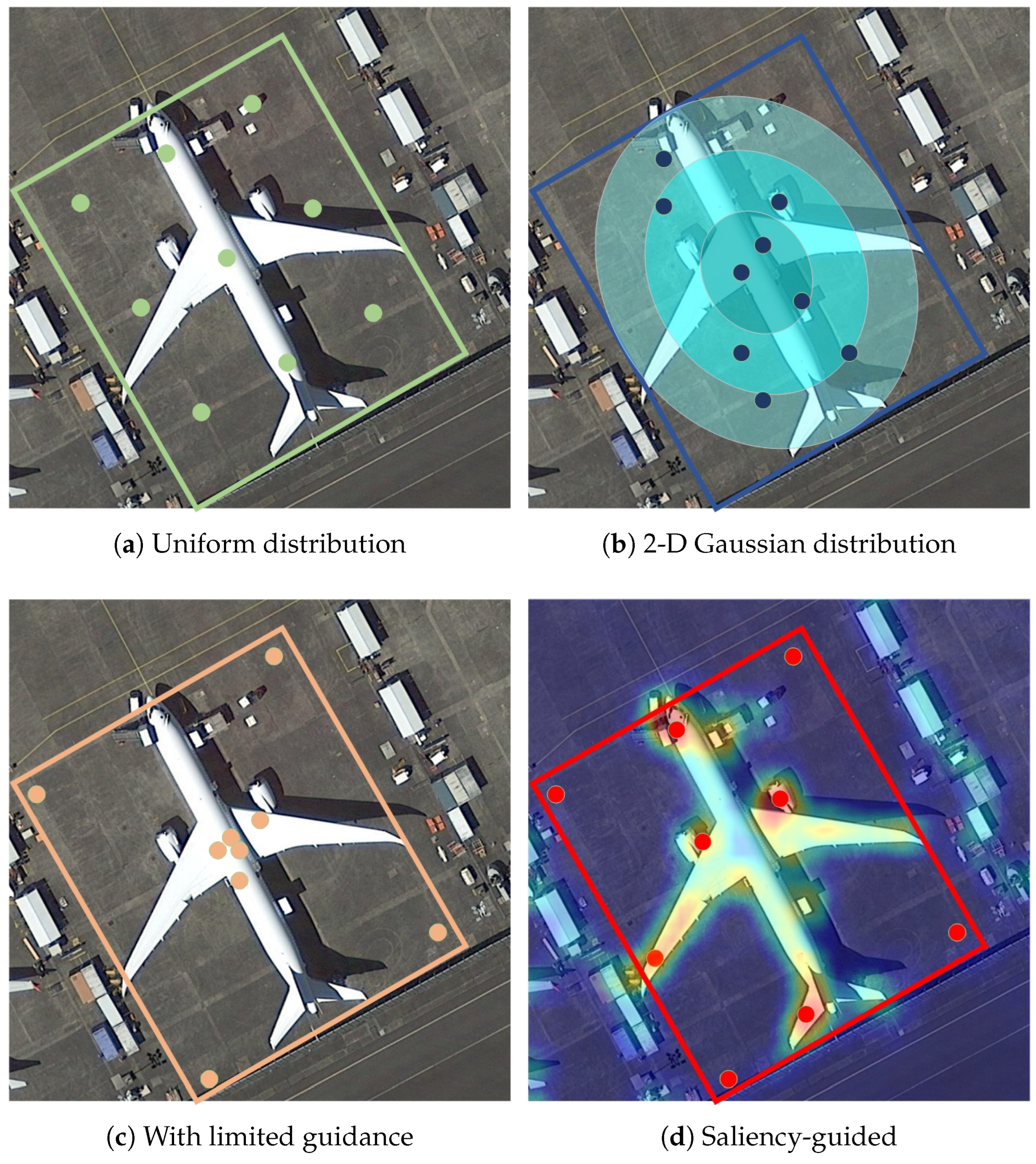
The offsets of DCN essentially represent collections of sampling points, which should follow a certain distribution pattern. To guide the selection of these sampling points, it is necessary to identify an effective distribution. For example, ordinary convolution can be viewed as sampling points following a fixed uniform distribution within a square. S²ANet [10] and AFRE-Net [15] incorporate an alignment module to rearrange the positions of sampling points, under the assumption that employing a scale-variable uniform sampling strategy can effectively capture accurate feature representations. However, this approach may encounter difficulties when dealing with non-rectangular objects, as some sampling points may inadvertently fall within the background region. Some researchers [16,17] posit that the sampling points adhere to a 2-D Gaussian distribution, with sampling conducted under a fixed distribution pattern where only the scale and orientation vary. The aforementioned assumptions that the distribution patterns of sampling point sets are constant for all targets and categories, with only the scale and orientation of the distribution varying, do not effectively adequately showcase the flexibility of DCN sampling. Conversely, some methods [18,19,20] assume that the sampling points can self-learn an appropriate distribution pattern based on the gradients backpropagated by the classification and localization loss functions. Different distribution patterns of sampling points are illustrated in Figure 1. However, our experiments reveal that the gradients backpropagated by the loss function are insufficient to enable the model to autonomously learn an efficient distribution pattern, thereby resulting in sampling points remaining in their initial position.

The shared issue among these methods lies in the inefficient distribution patterns of sampling points, caused by a lack of either effective or flexible guidance. This occurs as these methods focus solely on providing information about the ground truth boundaries for model learning, yet overlook the crucial internal information within these boundaries. The neglect of internal information from the objects within the ground truth boundaries hinders the accurate detection and understanding of remote sensing objects. In addition, the DCN should not be guided by forcefully imposing a specific distribution pattern on the sampling points, as this approach may result in misalignment between the spatial and feature domains [21,22]. Consequently, DCN offsets do not truly learn to acquire high-quality feature representations of the targets through accurate sampling, and the resulting feature representations may not be comprehensible to downstream predict heads. To mitigate misalignment between the spatial and feature domains, it is essential not only to guide the sampling points of the DCN to learn flexible and object-aware sampling patterns within the bounding box but also to implement strategic learning approaches. These approaches will enable the prediction module to effectively interpret the feature representations derived from the sampling points.

To address the issue previously mentioned, this study introduces Saliency-Guided RepPoints (SGR), a flexible and efficient framework for object detection, building upon the RepPoints method. Unlike other RepPoints-based methods, SGR utilizes saliency maps derived from ground truth data as guidance to learn and predict the positioning of sampling points. These response peaks frequently signify areas enriched with salient features. This enrichment allows the DCN to extract feature representations from those areas that are more distinctive and discriminative. In order to alleviate the potential misalignment between spatial and feature domains during the learning process, we propose a dynamic dual-alignment (DDA) training strategy, which incorporates the saliency-guided method. This strategy consists of two components: a label assigner and loss functions. By augmenting external salient information, which belongs to spatial information, a loss function can be used as a constraint to guide the prediction of DCN offsets to focus on these regions. The sampled feature representations belong to the feature domain information and need to be passed on to downstream regression and classification predict heads to obtain the final results. In order to gradually enable the predict heads to understand the feature representations from the upstream during the training process, we also consider both the spatial prior information of the sampled points and the posterior information from the downstream predictions simultaneously during the label assignment phase. During the training process, the label assigner can achieve a trade-off dynamically according to the matching measurements, thus alleviating the optimization difficulties caused by misalignment. Through training with DDA, the dual-alignment of spatial and feature domains can be achieved. Furthermore, in order to examine the alignment between feature representation and the classification performance of predict head, we propose an interpretable approach to validate the effectiveness of sampling points and provide a theoretical analysis. This visualization method has the characteristics of being intuitive and having finer granularity. Moreover, it is also applicable to other point-based methods.

According to the content presented above, the main contributions of this study can be summarized as follows:

• To enhance the accuracy of feature representation, we propose Saliency-Guided RepPoints, a method that utilizes information within bounding boxes to guide the learning of distribution patterns for DCN offsets.
• To alleviate the potential misalignment between the spatial and feature domains caused by model-guiding, we have designed a dynamic dual-domain alignment training strategy, which mitigates the optimization difficulties.
• We propose an interpretable visualization method to assist in validating the effectiveness of our proposed SGR.
• To validate the effectiveness of our proposed method, we conducted a series of experiments on four diverse and demanding datasets, namely, DOTA [23], HRSC2016 [24], DIOR-R [25], and UCAS-AOD [26].

The structure of this paper is as follows: Section 2 introduces related work, providing a brief overview of the status of research related to our work. Section 3 presents, in detail, our proposed method and its implementation. Section 4 demonstrates the effectiveness of the method through experimental results. Section 5 provides a theoretical discussion based on the experimental results, highlighting the effectiveness of our method and suggesting potential areas for improvement in future work. Finally, Section 6 summarizes the conclusions derived from our work.

2. Related Work

In this section, a thorough review is conducted of the existing literature relevant to remote sensing object detection, emphasizing specifically the feature representation of objects and dynamic assignment strategies. These aspects are intimately connected to the focus of our study.

2.1. Remote Sensing Object Detection

The task of object detection in remote sensing imagery involves the localization and classification of objects. Differing from object detection in other types of imagery, remote sensing images are characterized by distinct difficulties, including arbitrary orientation, dense packing, and complex backgrounds. In recent years, with the advancement of deep CNNs, many methods have been proposed for remote sensing object detection. These methods can be categorized into two major types: single-stage and two-stage methods. Due to the constraints of the CNN receptive field, achieving accurate localization is crucial for improving the performance of the model. To achieve more accurate localization, the two-stage paradigm first performs coarse localization [6,7,12], and then refines the localization and performs classification based on the coarse localization. This paradigm has achieved great success with excellent performance. Nevertheless, the two-stage paradigm also has its drawbacks, such as longer training time and larger memory consumption, which makes it unsuitable for lightweight end devices and real-time inference scenarios. Over the recent past, one-stage methods have made great progress, closing the performance gap with two-stage methods. Li et al. [20], as well as Han et al. [10], proposed the utilization of single-stage dense prediction offset, followed by the adoption of DCN-based offset sampling, to achieve superior localization performance without the time-consuming overhead associated with two-stage approaches. Additionally, the design of dense prediction in the single-stage paradigm enables high recall rates. Among them, point-based methods have attracted growing interest due to their flexible feature representation capabilities and high robustness in obtaining bounding boxes. Yang et al. were the pioneers in introducing the point-based RepPoints method, demonstrating that it is a geometric representation of objects that reflects more accurate semantic localization compared to traditional RoI-based methods [18]. Subsequent studies have adapted the RepPoints method [20,27,28,29,30] to the domain of remote sensing object detection, where the targets exhibit greater geometric and morphological variability. These studies have achieved commendable results, largely owing to the feature representation’s ability to capitalize on its flexibility to extract more precise features of the objects.

2.2. Feature Representation of Objects

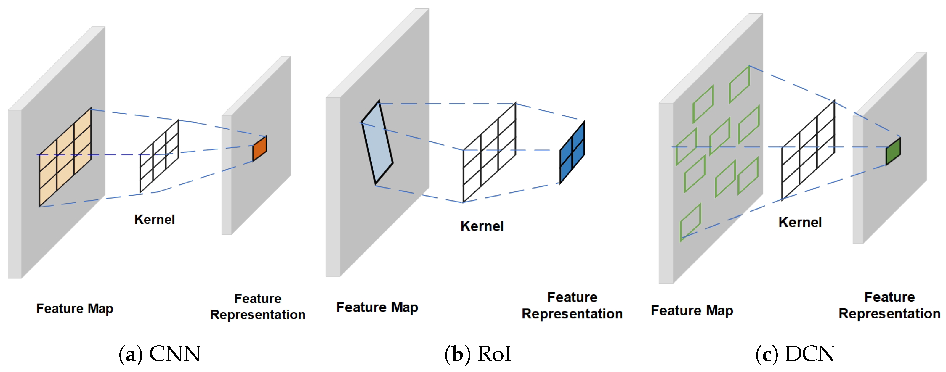
Remote sensing images undergo processing via a backbone network and a feature pyramid network (FPN), resulting in the generation of multi-scale feature maps. From these feature maps, essential feature domain information is extracted, constituting what we refer to as feature representation. The success of downstream tasks, specifically in localization and classification, relies heavily on the quality of this feature representation. It is evident that obtaining effective and crucial feature representation plays a vital role in enhancing the performance of remote sensing object detection. The traditional approach of using conventional convolutions, depicted in Figure 2a, for feature representation of objects with anchor-based axis-aligned square region sampling lacks flexibility, particularly in the case of remote sensing objects with arbitrary orientations, as it introduces substantial background noise. Xie et al. proposed refining oriented RoI [7], depicted in Figure 2b, utilizing a two-stage scheme to obtain feature representation of the same scale from regions of different sizes. This method resulted in remarkable improvements. The use of RoI for feature extraction requires an upstream region proposal network (RPN) module, and such two-stage methods consume lots of computational resources, resulting in slow inference speed. Therefore, in recent years, researchers have turned their attention to DCN, depicted in Figure 2c, which can also adaptively extract feature representations. Han et al. utilized a feature alignment module (FAM) [10] to align the location and orientation to obtain more accurate feature representations. Li et al. predicted key points from the feature map in the initial stage and used them as offsets for DCN [20]. Regarding the selective acquisition of sampling points, Hou et al. proposed shape-adaptive selection and measurement [14], while other studies assumed that the points followed a two-dimensional Gaussian distribution [16,17]. The feature representations obtained through the aforementioned different sampling methods will considerably influence downstream localization and classification tasks.

The feature representations obtained by the upstream sampling points will be passed on to the downstream prediction modules. Most existing methods for remote sensing object detection represent bounding boxes using five parameters $(x,y,w,h,\mathit{\theta })$, where x and y denote the coordinates of the center point, w and h represent the width and height, and theta represents the rotation angle. These parameters are directly predicted by the regression method employed in the predict head and subsequently refined using the SmoothL1 loss. However, directly introducing an additional angular parameter to the output of a horizontally aligned bounding box results in imprecise predictions, which, in turn, diminishes the overall performance of the model. One common issue is the discontinuity in the angle regression loss. Several methods [31,32,33,34], such as that of Yu et al., propose an innovative phase-shifting coder that encodes the angle of orientation to effectively mitigate the problem of bounding box discontinuity [35], but they still fail to completely eliminate this problem. Another approach to obtain bounding boxes apart from direct regression is by utilizing points. A notable method in this field is RepPoints [18,20], which is a generic detector that leverages point extraction to obtain key features. Specifically, a set of representation points is generated for each pixel in the feature maps. By integrating the acquired offsets as prior information, the DCN is utilized to sample the neighborhood regions. Following this, two parallel branches are utilized, one for classification and the other for refinement. The refined results are then transformed into bounding boxes using a conversion function [20,30]. The existing RepPoints method operates under the assumption that the learning of an adaptive point-set can be self-guided by downstream classification and regression tasks [18,20,28], which are, in turn, supervised by the loss function. Unfortunately, such weak guidance is inadequate, leading to an unreasonable distribution of sampling points.

It is evident that obtaining accurate feature representations is crucial for achieving optimal results. Nevertheless, the aforementioned DCN-based methods often fail to recognize the importance of directing the distribution patterns in sampling. This aspect merits further investigation, given its potential influence on the performance of detection.

2.3. Dynamic Assignment Strategies

The assignment of positive and negative labels to samples plays a crucial role in supervising the learning process of the model in the field of deep learning and remote sensing object detection. Traditional object detection approaches typically use intersection over union (IoU) as a measurement and a fixed hyperparameter as a threshold. However, the adaptive training sample selection (ATSS) [36] method continuously adjusts the assigned IoU threshold during the model learning process. Additionally, the dynamic anchor learning (DAL) [37] approach incorporates consideration of classification and regression, utilizing the matching degree to dynamically assign labels. Furthermore, Xu et al. proposed the finer dynamic posterior matching method [17], which incorporates posterior information into the evaluation metric to better capture the shape of objects. Furthermore, it is worth investigating the assignment strategy of the transformer-based detection transformer (DETR). Some studies [38] have demonstrated that the Hungarian matching implementation of the DETR, which achieves one-to-one high-quality matching, significantly improves performance. Researchers such as Li et al. [39] and Zhang et al. [40] have incorporated the advantages of Hungarian matching into CNN-based models.

In short, it is crucial to obtain accurate feature representations when it comes to object detection in remote sensing. The use of DCN in single-stage methods has demonstrated their high accuracy and computational efficiency. Nonetheless, the DCN’s offset still needs effective guidance to minimize the ambiguity of the obtained feature representation. Moreover, high-quality labels are indispensable for training; thus, a label assigner customized to the detector’s characteristics is necessary to fully leverage its performance.

3. Method

This section offers a comprehensive overview of the methodology employed to direct the DCN towards extracting high-quality feature representations. Furthermore, it elaborates on the approach to achieve dual alignment through dynamic label assignment, covering both the design rationale and the underlying theoretical framework.

3.1. Overview of Proposed Method

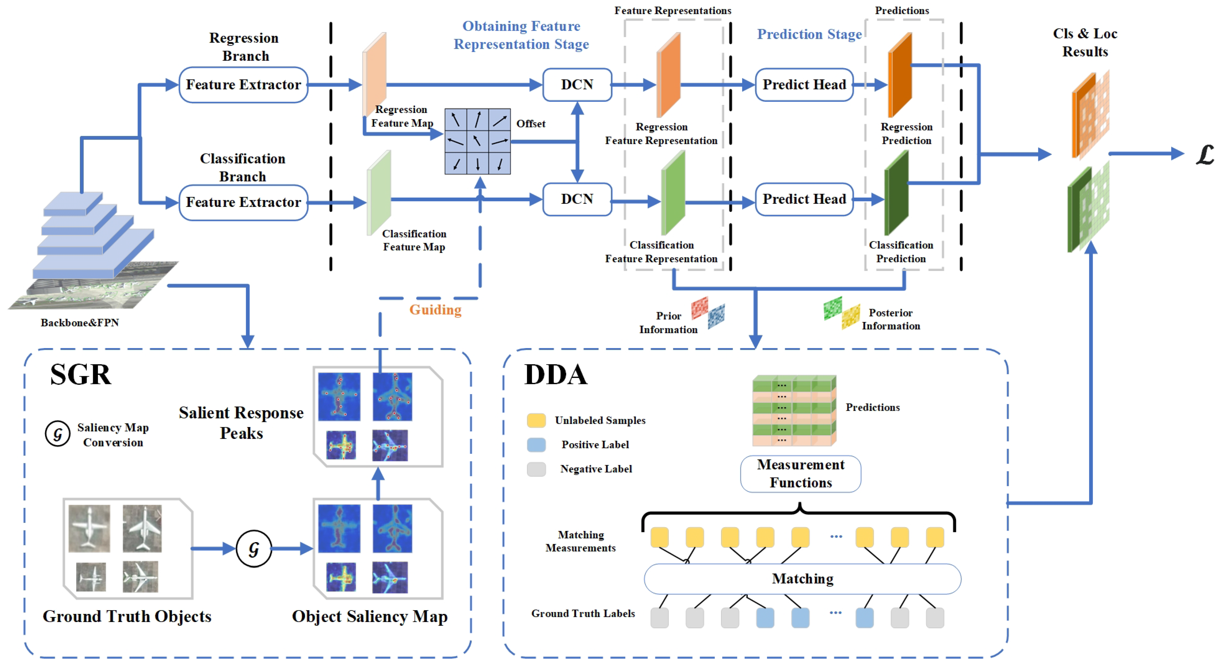
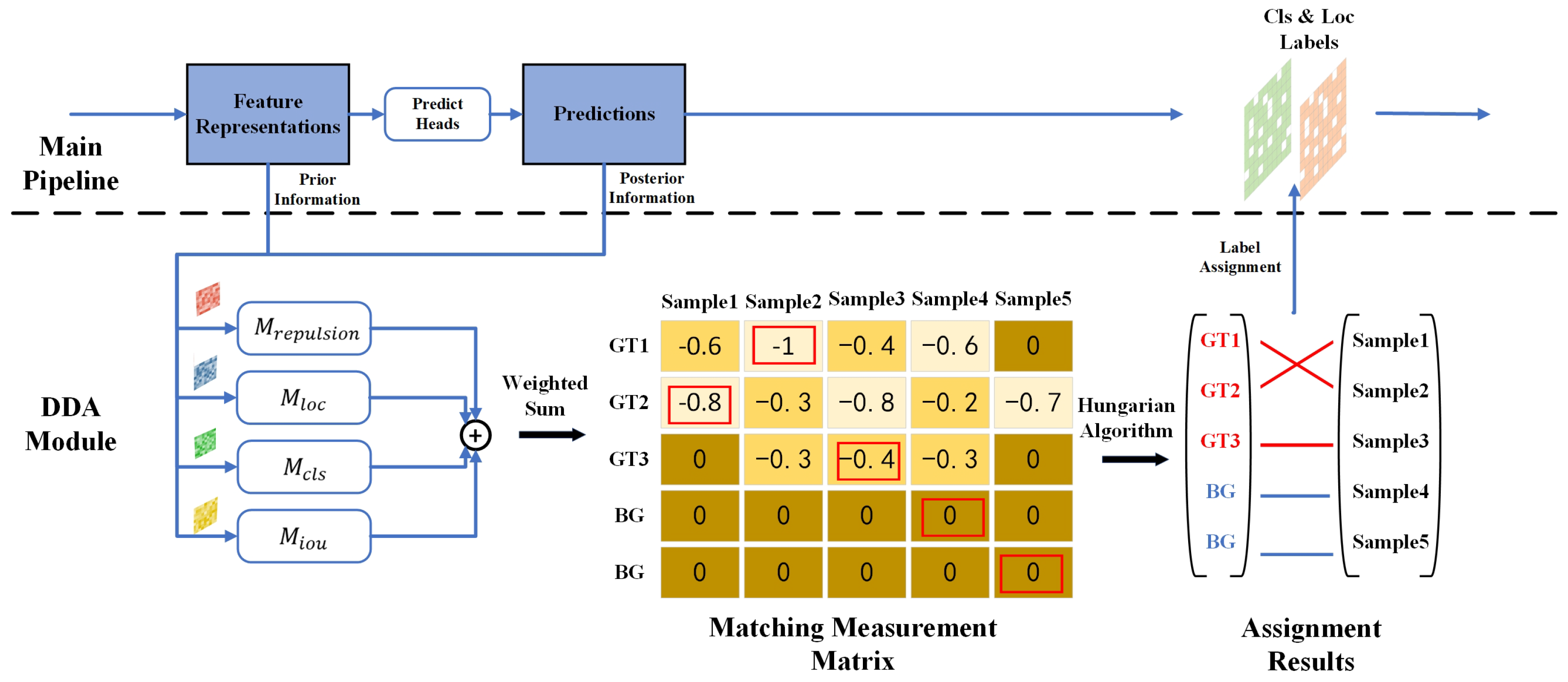
The overall pipeline is visualized in Figure 3. A remote sensing image is initially processed by a backbone network for feature extraction, followed by the use of FPN to obtain five feature maps of different scales, namely, $\left[F_n\right|n=3,4,5,6,7]$. In the detection pipeline, we focus on two key stages, namely, the obtaining feature representation stage and the prediction stage. To address this, we employ the deformable convolution inherited from RepPoints to sample the key regions predicted by the model. This approach allows us to utilize different sampling modes for different objects, thereby obtaining a more accurate shape-adaptive feature representation of the objects. Moreover, we employ saliency maps to explore regions in the ground truth images that may contain important information, guiding the sampled points to focus on these areas. To obtain high-quality positive and negative samples and to avoid misalignment between spatial and feature domains, we incorporate prior knowledge and posterior knowledge of the model into the matching alignment degree and utilize the Hungarian matching algorithm to complete label assignment. Furthermore, based on the label assignment results, we filter out low-quality samples, and subsequently pass the filtered samples into the loss function to compute the loss and backpropagate the gradients for optimizing the model parameters.

3.2. Sampling Points Distribution Pattern

The DCN calculates the feature representation of the objects at each pixel on the feature maps by utilizing the contextual information of its neighborhood. To enable the model to obtain shape-adaptive feature representation, we predict the offset of a sampled keypoint set at each pixel on the feature map, which represents the distribution pattern of sampling points, denoted as P.

$$P_i(x,y)=I\left(F_i(x,y)\right)={\left\{(\Delta x_j,\Delta y_j)\right\}}_{j=1}^n,i=3,4,5,6,7$$

(1)

In the Equation (1) above, $F_i$ designates the feature map of the $i^{th}$ layer, while i signifies a neural network predicting the point set patterns, which is composed of multiple superimposed neurons. I is a function that predicts the sampling points based on the pixels on the feature map. $P_i$ refers to the point set pattern obtained on the ith feature map.

The underlying principle of the distribution pattern of sampling points lies in how the model interprets features at a specific pixel. It determines the neighboring regions that contain important information and the information it desires to know. A pattern not only includes the positional information of a set of points, but also contains predictions about the geometric features, shape characteristics, size, rotation angle, and so on, implied by the relative positions of the points in the set. The specific predictions depend on the nature of the object and its class.

We incorporate the predicted P as the offset and employ a DCN to extract shape-adaptive feature representations of the target.

$$R_i(x,y)=\sum _{j=1}^K{w}_j\ast F_i\left(x+\Delta x_j,y+\Delta y_j\right)$$

(2)

In Equation (2), $R_i$ represents the feature representation, which is obtained by summing the weighted contributions. The weights, $w_j$, represent the importance of each neighboring pixel’s feature contribution. Each pixel’s feature contribution, $F_i(x+\Delta x_j,y+\Delta y_j)$, is computed by evaluating the feature map at a shifted position, $(x+\Delta x_j,y+\Delta y_j)$, relative to the current pixel’s position $(x,y)$. Specifically, we partition the feature sampling process into two independent branches, namely the regression branch and the classification branch, based on the downstream prediction tasks. This dual-branch design enhances the stability of the model by allowing for separate feature maps dedicated to regression and classification tasks. The offset can be added to a base offset, such as $B=\left\{\right(-1,-1),(-1,0),...,(0,1),(1,1\left)\right\}$, allowing it as knowledge, or it can be left out for the model to learn autonomously. In deformable convolution, the parameter w signifies the model’s comprehension of the characteristics of each sampled point. This includes the model’s varying degrees of attention to distinct features. In practical applications, the points within a given set may assume varied functional roles. For instance, certain points may be primarily tasked with discerning the object’s edges and background, whereas others may focus on comprehending the central attributes of the object. The following provides a comprehensive and detailed explanation.

3.3. Saliency-Guided RepPoints (SGR)

The SGR offers an intuitive method for directing the model’s sampling points, addressing the inadequacies of the existing RepPoints method that relies solely on gradients backpropagated from the classification and regression subtasks. These subtasks primarily extract information about the bounding box from the ground truth but fall short in efficiently mining the intricate details within it. This limitation necessitates an additional source of information to guide the DCN in adopting an appropriate sampling distribution pattern. Such guidance is crucial for the DCN to attain a superior quality of object feature representation.

Saliency maps methods, renowned for their effectiveness in pixel-level object detection and fine-grained classification, provide granular and interpretable visual insights. They are adept at highlighting crucial information within bounding boxes. Thus, in the SGR framework, we leverage the positional information obtained from saliency maps to guide the RepPoints sampling process. This integration of saliency information into the point guidance is a key aspect of SGR. Such a method significantly enhances the RepPoints’ ability to capture the essential features and patterns across different object categories. Consequently, SGR fosters a more nuanced and precise detection process by leveraging detailed insights of objects.

$$s_n=\mathcal{S}\left(t_n\right),n=1,2\dots$$

(3)

Equation (3) illustrates the process. Here, $t_n$ denotes the nth ground truth target image, and $s_n$ represents its corresponding saliency map, which is a grayscale image. The function $\mathcal{S}$, signifying an algorithm, converts an RGB image into a saliency map. We employ the method of spectral residual, as cited in [41], to generate static saliency maps. Typically, areas on a saliency map with stronger responses indicate regions more likely to capture human attention. Consequently, from a human-centric viewpoint, salient points are expected to coincide with these peak response regions on the saliency map. Extracting these key points is vital to guide the model in identifying these areas. Deformable convolution is utilized to derive feature representations with enhanced interpretability from these regions.

$$P^{guidance}=FindPeak\left(s\right)=\{p_n\mid n=1,2\dots ,K\}$$

(4)

Equation (4) denotes the top K peaks with the highest response values on the saliency map. A local maximum filtering algorithm is employed to identify these peaks, allowing for the isolation of the most representative regions within each ground truth target. These P points, combined with the boundary information of the target ground box, enrich the dataset, facilitating model learning. A specialized loss function guides the predicted sampling points towards the $P^{guidance}$ region. This approach is conceptualized as an optimization problem aiming to minimize the distance between two point sets. For this purpose, we utilize the Chamfer distance as a measure for quantifying the disparity between two point sets.

$$\begin{array}{c}\hfill {\mathcal{F}}_{ChamferDist.}(P,P^{guidance})=\frac{1}{\left|P\right|}\sum _{x\in P}\underset{y\in P^{guidance}}{min}{\parallel x-y\parallel }_2^2\\ \hfill +\frac{1}{\left|P^{guidance}\right|}\sum _{x\in P^{guidance}}\underset{y\in P}{min}{\parallel x-y\parallel }_2^2\end{array}$$

(5)

Equation (5), ${\mathcal{F}}_{ChamferDist.}(P,P^{guidance})$ quantifies the Chamfer distance between two sets of points, where P represents the pattern of sampling points predicted by the model, and $P^{guidance}$ denotes the predetermined guiding point set. This loss function is specifically designed to steer the model towards predicting a pattern of sampling points that closely aligns with the guiding point set. Importantly, it should be noted that the number of elements in the two point sets need not be identical. This flexibility is integral to the function’s application, accommodating varying quantities of points in each set while still providing a reliable measure of similarity between them. This metric will serve as a component of the loss function, with our proposed overall loss function defined as follows:

$$\mathcal{L}={\mathit{\lambda }}_1{\mathcal{L}}_{\mathrm{loc}}+{\mathit{\lambda }}_2{\mathcal{L}}_{\mathrm{cls}}+{\mathit{\lambda }}_3{\mathcal{L}}_{\mathrm{guidance}},$$

(6)

where

$${\mathcal{L}}_{\mathrm{cls}}=\frac{1}{N_{\mathrm{cls}}}\sum _i{\mathcal{F}}_{\mathrm{focal}}(P_i^{\mathrm{cls}},g_i^{\mathrm{cls}}),$$

(7)

$${\mathcal{L}}_{\mathrm{loc}}=\frac{1}{N_{\mathrm{loc}}}\sum _i{\mathcal{F}}_{\mathrm{ciou}}(P_i^{\mathrm{loc}},g_i^{\mathrm{loc}}),$$

(8)

$${\mathcal{L}}_{\mathrm{guidance}}=\frac{1}{N_{\mathrm{loc}}}\sum _i{\mathcal{F}}_{\mathrm{ChamferDist}.}(P_i^{\mathrm{loc}},P_i^{\mathrm{guidance}}).$$

(9)

In Equations (6)–(9), $N_{\mathrm{cls}}$ and $N_{\mathrm{loc}}$ represent the total number of positive samples for classification and localization, respectively. $P_i^{\mathrm{cls}}$ denotes the predicted class score based on the feature representation, and $P_i^{\mathrm{loc}}$ signifies the positional coordinates of the predicted points set. $g_i^{\mathrm{cls}}$ represents the ground truth classification information for the $i^{th}$ target and $g_i^{\mathrm{loc}}$ signifies the ground truth positional information of the $i^{th}$ target. ${\mathcal{F}}_{\mathrm{ciou}}$ is the convex IoU loss.

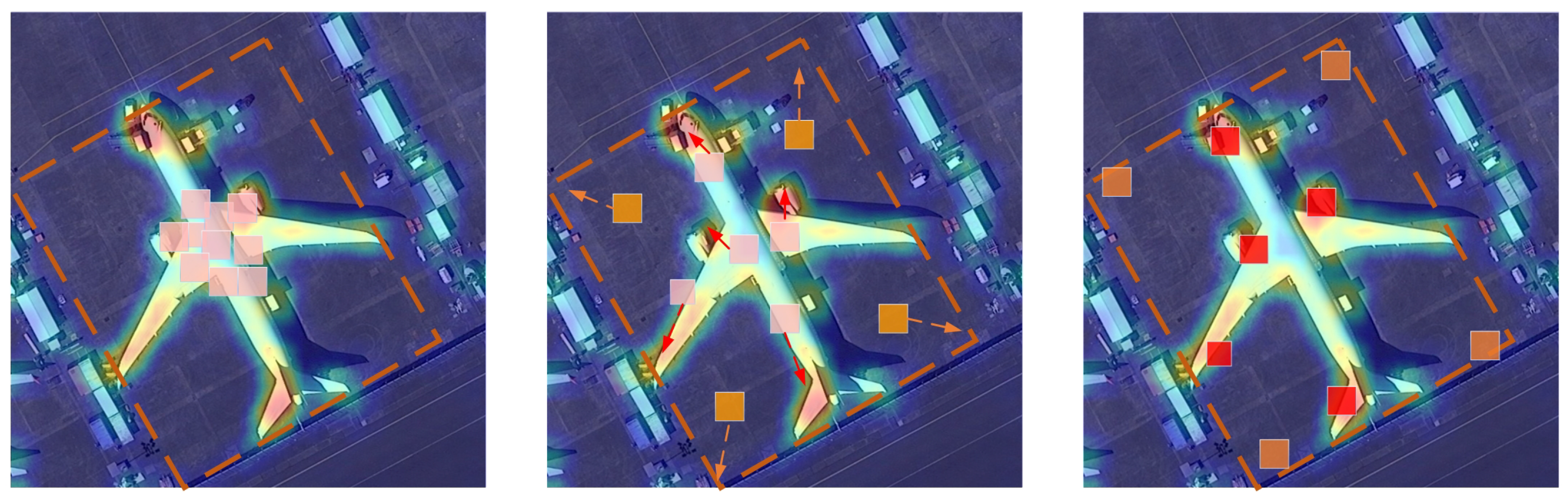
During the training process with SGR, guided by the saliency map and convex IoU loss, the sampled points acquire different roles. Some points are responsible for exploring the boundaries, while others focus on identifying more distinguishable features on the targets, as shown in Figure 4. As the training progresses, the division of labor among different sampled points becomes clear, and the obtained feature representation gradually stabilizes. This phenomenon can be attributed to the exploitation of the saliency map for highlighting important regions and the convex IoU loss for encouraging the accurate localization of objects.

3.4. Dynamic Dual-Domain Alignment (DDA) Assignment

DDA, a training strategy innovatively redeveloped based on the SGR framework, is illustrated in Figure 5. It employs the combined use of prior and posterior information as a matching measurement, providing high-quality label assignments. This approach assists SGR in circumventing potential misalignments between the spatial and feature domains. DDA is designed to complement the SGR by directing sampling points towards regions of higher saliency within the ground truth bounding boxes, thus focusing the model’s attention in the spatial domain. A concern arises when sampling points, constrained by loss functions, do not learn the correct distribution patterns effectively. Such constraints can hinder the downstream predict heads from interpreting the feature representations provided by the DCN, despite their inherent accuracy and desirability. This discrepancy may lead to a disconnection between the spatial and feature domains. To address these challenges and to reduce confusion in the model’s learning process, we have redesigned the label assignment strategy. This revised strategy aims to establish a more effective balance between the model’s inherent learning mechanisms and the input from the sampling points, thereby enhancing the model’s overall prediction accuracy.

The predictive output of a model reflects its learning outcomes, and this becomes particularly evident in the later stages of training. As training progresses, the distribution pattern of the sampling points stabilizes, indicating that the feature representations acquired by the DCN experience minimal changes. Consequently, the primary focus of optimization shifts to the prediction stage, with the feature representation considered as a given and the predict head as an optimizable entity. The effectiveness of the model’s predictions serves as a measure of the predict head’s understanding of the feature representation—better predictions imply a deeper comprehension. To align the learning processes in the spatial domain, where sampling occurs, with those in the feature domain, where understanding is developed, it is crucial to dynamically adjust the label assignment strategy throughout different learning phases. This strategy integrates the model’s predictive performance as a posterior criterion into our assignment measurement, alongside prior information, such as the model’s initial positioning. Such an approach is designed to achieve spatial and feature alignment during the model’s training process.

For an input image, the assignment measurement for each proposal corresponding to each ground truth object is calculated as follows:

$$M_{total}={\mathit{\mu }}_1{M}_{cls}+{\mathit{\mu }}_2{M}_{iou}+{\mathit{\mu }}_3{M}_{loc}+{\mathit{\mu }}_4{M}_{repulsion}$$

(10)

where

$$\begin{array}{cc}\hfill M_{cls}& ={\mathcal{F}}_{focal}(P_i^{cls},g_j^{cls}),\hfill \\ \hfill M_{iou}& ={\mathcal{F}}_{ciou}(P_i^{loc},g_j^{loc}),\hfill \\ \hfill M_{loc}& ={\mathcal{F}}_{smoothF1}(B_i^{loc},g_j^{loc}).\hfill \end{array}$$

(11)

In the Equation (10), $M_{cls}$ and $M_{iou}$ represent posterior information, whereas $M_{loc}$ and $M_{repulsion}$ are related to prior spatial information. The costs are all negative. The term $B_i^{loc}$ denotes the center position of the rectangular box obtained by transforming the i-th prediction using the minAreaRect function. The definition of $M_{repulsion}$ is as follows:

$$M_{repulsion}=-e^{-\mathit{\alpha }{\sum }_{1\le y<x\le K}{\parallel P_x-P_y\parallel }_2^2}$$

(12)

The term $M_{repulsion}$, as defined in Equation (12), is formulated to discourage the excessive clustering of the sampling points. In this expression, $P_x$ and $P_y$ denote distinct points within the point set. The parameter $\mathit{\alpha }$ serves as a hyperparameter, modulating the decay rate of this measure as the dispersion of the point set increases. The hyperparameters ${\mathit{\mu }}_1$, ${\mathit{\mu }}_2$, ${\mathit{\mu }}_3$, and ${\mathit{\mu }}_4$ in the equation are used to balance these various measures. All the measurements are negative. Assuming there are n proposals and m ground truths, M is an $n\times m$ assignment measurement matrix. Through the Hungarian algorithm, we minimize the matching measurement, expressed as follows:

$$\widehat{\mathit{\sigma }}=arg\underset{\mathit{\sigma }\in {\mathit{\Sigma }}_N}{min}\sum _{i=1}^{N}M(P_{\mathit{\sigma }\left(i\right)},g_i)$$

(13)

In Equation (13), $\widehat{\mathit{\sigma }}$ represents the matching result and ${\mathit{\Sigma }}_N$ denotes the solution space for matching. The term $P_{\mathit{\sigma }\left(i\right)}$ refers to the samples matched to $g_i$, the i-th ground truth. Since the number of predicted P’s is generally more than that of $g_i$’s, the matrix M is made square by padding with zeros to ensure that both P and g can be matched. In $\widehat{\mathit{\sigma }}$, matches to the actual ground truths are considered positive samples, while matches to the padded zeros are considered negative samples.

DDA provides the model with high-quality positive samples that consider posterior information, thus reducing confusion during the learning process, as demonstrated in Figure 6. This method guides the assigner to emphasize different aspects during model training. Initially, when the model exhibits weak classification capabilities, greater emphasis is placed on the location of proposals to enhance the learning of salient feature representations. As the model’s localization ability strengthens, the focus gradually shifts to improving the classification accuracy. Specifically, the objective is to optimize the weights to minimize classification confusion given a feature representation. Ultimately, this approach enables the model not only to identify suitable feature representations but also to enhance classification based on these representations, leading to improved overall predictions.

3.5. Point Local Interpretable Map

In order to validate the alignment efficacy of DDA, particularly in terms of the predict head’s assessment of the sampling points’ positions, we introduce a method for interpretable visualization. This approach concentrates on evaluating the rationality of the sampling points’ positions through visualization techniques. Our method is founded on the fundamental mathematical concept that the final classification predict head can be conceptualized as a multivariate function, defined as:

$$SCORE=\mathcal{H}(p_1,p_2,p_3,\dots ,p_K)$$

(14)

In Equation (14), $SCORE$ represents the classification scores from the classification branch. The function $\mathcal{H}$ symbolizes the computation of the classification predict head, encompassing the positions of the sampling points $(p_1,p_2,p_3,\dots ,p_K)$.

Given that H in a trained model is a fixed, deterministic function and that deformable convolution employs linear interpolation in the sampling process, we posit that H can be approximated as a continuous function [8]. Analogous to how the variation of a multivariate function can be gauged by observing increments in its vicinity, the changes in SCORE upon slight adjustments of the sampling points, denoted as $\mathit{\delta }$ in Equation (15), offer insights into the model’s comprehension of the feature representation patterns:

$$\Delta SCORE=\mathcal{H}(p_1+\mathit{\delta },p_2,p_3,\dots ,p_K)-\mathcal{H}(p_1,p_2,p_3,\dots ,p_K)$$

(15)

In an ideal scenario, the feature representations derived from sampling based on predicted points should be coherent and interpretable by the downstream predict heads. Theoretically, displacing a sampling point within its neighborhood is expected to result in a decline in classification confidence, indicating that the original position of the sampling point represents a function’s extremum. By analyzing changes in $\Delta SCORE$, we can deduce whether the model’s predict head corroborates the appropriateness of the predicted sampling points. Additionally, this approach facilitates the detection of potential misalignments through visual inspection. In practice, this methodology involves systematically shifting the focal sampling point across a neighboring grid. This approach facilitates a comprehensive examination of how such movements affect the classification scores.

4. Experiments and Results

In this section, the four publicly available datasets utilized in our experiments are first introduced, followed by a discussion on the implementation details and evaluation metrics. Subsequently, the experimental results are presented, aimed at validating the effectiveness of the proposed method.

4.1. Datasets

In order to validate the effectiveness of our proposed method, we conducted a series of experiments on four diverse and demanding datasets, namely, DOTA [23], HRSC2016 [24], DIOR-R [25], and UCAS-AOD [26]. These datasets were specifically chosen as they represent different challenges and characteristics commonly encountered in remote sensing object detection tasks.

DOTA is one of the most authoritative large-scale datasets for object detection in aerial images. It consists of fifteen categories, namely ’plane’, ’baseball-diamond’, ’bridge’, ’ground-track-field’, ’small-vehicle’, ’large-vehicle’, ’ship’, ’tennis-court’, ’basketball-court’, ’storage-tank’, ’soccer-ball-field’, ’roundabout’, ’harbor’, ’swimming-pool’, and ’helicopter’, which will be abbreviated as PL, BD, BR, GTF, SV, LV, SH, TC, BC, ST, SBF, RA, HA, SP, and HC, respectively. The dataset employs rotated bounding box annotations, encompassing dense, complex backgrounds, arbitrary orientations, and other challenging scenarios. The DOTA dataset comprises a total of 2806 remote sensing images, each varying in size from 800 × 800 to 4000 × 4000 pixels. The dataset is further divided into three distinct sets: a training set, a validation set, and a testing set, which are presented in proportions of 1/2, 1/6, and 1/3, respectively, or numerically, 1411, 458, and 937 images in the respective sets. For the purpose of our experiments, we utilize both the training and validation sets in order to train the proposed detector. To this end, all the images used for training are segmented into patches of 1024 × 1024 pixels, with a stride of 200 pixels. As part of the rigorous data augmentation techniques, we also employed random resizing and flipping, aiming to enhance the robustness of the model.

The HRSC2016 dataset operates with the oriented bounding box annotation method. Designed as a high-resolution dataset, the HRSC2016 exhibits a resolution ranging from 0.4 m to 2 m. Specifically, all images within this dataset are sourced from six renowned ports and incorporate an array of seafaring vessels along the coast. The size of the ship images varies from 300 to 1500, with most of the images exceeding dimensions of 1000 × 600. Additionally, this dataset is constituted of three different segments: a training set embracing 436 images (with 1207 samples), a validation set encompassing 181 images (with 541 samples), and a testing set comprising 444 images (with 1228 samples). As a part of our research, we resized all the images to an 800 × 512 resolution and applied random horizontal flipping as an augmentation strategy to enhance the diversity of the model’s training data.

The DIOR-R dataset is annotated using the oriented bounding box method and stands as a substantial benchmark dataset for object detection in optical remote sensing images. It is noteworthy that this dataset consists of instances spread across 20 different categories, thus providing a wide spectrum of scenarios for detection. All the images in this dataset have been resized to a standard dimension of 800 × 800, yielding a resolution that ranges between 0.5 and 30 m. The images were extracted from Google Earth, resulting in a total count of 23,463 images and comprising approximately 190,288 distinct objects.

The UCAS-AOD dataset, specializing in the detection of aircraft and automobiles, encompasses a total of 2420 images and 14,596 instances. The dataset consists of two classes, cars and airplanes, along with a background class serving as negative examples. Specifically, a total of 1000 images are automobile-based, comprising 7114 car instances, while, 7482 instances are designated towards aircraft illustrations. The defined distribution for the dataset allocation involves a ratio of 5:2:3 among the training, validation, and testing sets, respectively.

4.2. Implementation Details

We execute all the experiments on a computing system equipped with two Nvidia GeForce RTX 4090 GPUs, manufactured by Nvidia Corporation GPUs (Santa Clara, CA, USA), using a batch size of 8. For implementation, the open-source toolboxes MMRotate and MMDetection are employed. Furthermore, we opt for ResNet-50 and ResNet-101 as the backbone network architectures, incorporating FPN. It is noteworthy that the weights for these networks are pretrained and sourced from torchvision. For the learning process, we employ the stochastic gradient descent algorithm as our optimizer, featuring a learning rate of 0.01, momentum of 0.9, and weight decay set at 0.0001. Moreover, we methodically train our neural architecture, running for 40 epochs on DOTA, 120 epochs on HRSC2016, 40 epochs on DIOR-R, and 40 epochs on UCAS-AOD, respectively. The hyperparameters were set as follows: ${\mathit{\lambda }}_1$, ${\mathit{\lambda }}_2$, and ${\mathit{\lambda }}_3$ were, respectively, set to 1.0, 0.375, and 0.2. The values of ${\mathit{\mu }}_1$, ${\mathit{\mu }}_2$, ${\mathit{\mu }}_3$, and ${\mathit{\mu }}_4$ were set to 2, 2, 5, and 2, respectively. Furthermore, $\mathit{\alpha }$ was set to 1.5.

To assess the effectiveness of our proposed method, we employ the mean average precision (mAP) as the evaluation metric, a standard in the field of remote sensing object detection. The mAP is derived by computing the mean of the average precision (AP) values across all classes, defined as follows [42]:

$$mAP=\frac{1}{N}\sum _{i=1}^{N}A{P}_i$$

(16)

In Equation (16), N represents the number of classes, and $A{P}_i$ denotes the average precision for the i-th class. The AP is calculated as the area under the precision–recall curve for each class, representing a balance between precision (the proportion of correct positive predictions) and recall (the proportion of actual positives that were correctly identified). This metric effectively encapsulates the performance of an object detection model in terms of both accuracy and reliability.

4.3. Comparing Methods and Results

The performance evaluation on the DOTA dataset is presented in

Table 1. Experiment results on the DOTA dataset compared with state-of-the-art methods. Experimental results with best performance in red, second best in blue.

Method	Backbone	PL	BD	BR	GTF	SV	LV	SH	TC	BC	ST	SBF	RA	HA	SP	HC	mAP (%)
single-stage
RetinaNet-O [43]	R-50-FPN	88.67	77.62	41.81	58.17	74.58	71.64	79.11	90.29	82.18	74.32	54.75	60.60	62.57	69.67	60.64	68.43
DAL [37]	R-101-FPN	88.61	79.69	46.27	70.37	65.89	76.10	78.53	90.84	79.98	78.41	58.71	62.02	69.23	71.32	60.65	71.78
RSDet [44]	R-152-FPN	90.10	82.00	53.80	68.50	70.20	78.70	73.60	91.20	87.10	84.70	64.30	68.20	66.10	69.30	63.70	74.10
R3Det [45]	R-152-FPN	89.49	81.17	50.53	66.10	70.92	78.66	78.21	90.81	85.26	84.23	61.81	63.77	68.16	69.83	67.17	73.74
S2A-Net [10]	R-50-FPN	89.11	82.84	48.37	71.11	78.11	78.39	87.25	90.83	84.90	85.64	60.36	62.60	65.26	69.13	57.94	74.12
R3Det-DCL [34]	R-152-FPN	89.78	83.95	52.63	69.70	76.84	81.26	87.30	90.81	84.67	85.27	63.50	64.16	68.96	68.79	65.45	75.54
AFRE-Net [15]	R-101-FPN	89.34	85.74	53.23	75.96	79.22	81.03	87.88	90.86	83.82	87.08	65.95	67.33	76.52	73.06	64.52	77.44
two-stage
Faster-RCNN-O [2]	R-50-FPN	88.44	73.06	44.86	59.09	73.25	71.49	77.11	90.84	78.94	83.90	48.59	62.95	62.18	64.91	56.18	69.05
CAD-Net [46]	R-101-FPN	87.80	82.40	49.40	73.50	71.10	63.50	76.60	90.90	79.20	73.30	48.40	60.90	62.00	67.00	62.20	69.90
SCRDet [47]	R-101-FPN	89.98	80.65	52.09	68.36	68.36	60.32	72.41	90.85	87.94	86.86	65.02	66.68	66.25	68.24	65.21	72.61
FAOD [48]	R-101-FPN	90.21	79.58	45.49	76.41	73.18	68.27	79.56	90.83	83.40	84.68	53.40	65.42	74.17	69.69	64.86	73.28
RoI-Trans. [12]	R-101-FPN	88.65	82.60	52.53	70.87	77.93	76.67	86.87	90.71	83.83	82.51	53.95	67.61	74.67	68.75	61.03	74.61
Gliding-Vertex [49]	R-101-FPN	89.64	85.00	52.26	77.34	73.01	73.14	86.82	90.74	79.02	86.81	59.55	70.91	72.94	70.86	57.32	75.02
MaskOBB [50]	R-50-FPN	89.61	85.09	51.85	72.90	75.28	73.23	85.57	90.37	82.08	85.05	55.73	68.39	71.61	69.87	66.33	74.86
CenterMap [51]	R-50-FPN	88.88	81.24	53.15	60.65	78.62	66.55	78.10	88.83	77.80	83.61	49.36	66.19	72.10	72.36	58.70	71.74
ReDet [52]	ReR-50-ReFPN [52]	88.79	82.64	53.97	74.00	78.13	84.06	88.04	90.89	87.78	85.75	61.76	60.39	75.96	68.07	63.59	76.25
Oriented R-CNN [7]	R-101-FPN	88.86	83.48	55.27	76.92	74.27	82.10	87.52	90.90	85.56	85.33	65.51	66.82	74.36	70.15	57.28	76.28
anchor-free
CenterNet-O [53]	DLA-34 [53]	81.00	64.00	22.60	56.60	38.60	64.00	64.90	90.80	78.00	72.50	44.00	41.10	55.50	55.00	57.40	59.10
PIoU [54]	DLA-34	80.90	69.70	24.10	60.20	38.30	64.40	64.80	90.90	77.20	70.40	46.50	37.10	57.10	61.90	64.00	60.50
O2-DNet [55]	H-104 [56]	89.31	82.14	47.33	61.21	71.32	74.03	78.62	90.76	82.23	81.36	60.93	60.17	58.21	66.98	61.03	71.04
DRN [57]	H-104	89.71	82.34	47.22	64.10	76.22	74.43	85.84	90.57	86.18	84.89	57.65	61.93	69.30	69.63	58.48	73.23
CFA [58]	R-101-FPN	89.26	81.72	51.81	67.17	79.99	78.25	84.46	90.77	83.40	85.54	54.86	67.75	73.04	70.24	64.96	75.05
G-Rep. [16]	R-50-FPN	87.76	81.29	52.64	70.53	80.34	80.56	87.47	90.74	82.91	85.01	61.48	68.51	67.53	73.02	63.54	75.56
Oriented Rep. [20]	R-101-FPN	89.53	84.07	59.86	71.76	79.95	80.03	87.33	90.84	87.54	85.23	59.15	66.37	75.23	73.75	57.23	76.52
SGR(Ours)	R-50-FPN	87.53	84.64	57.78	73.78	79.40	77.61	86.58	90.91	85.49	85.30	63.52	71.05	73.61	69.50	66.59	76.88
SGR(Ours)	R-101-FPN	87.52	85.10	57.92	74.67	79.78	78.21	87.31	91.67	86.16	85.87	63.01	70.90	76.08	69.87	67.41	77.55
SGR(Ours)	Swin-T-FPN	87.58	86.67	61.04	74.53	79.99	79.10	87.13	90.85	84.48	87.04	62.51	75.00	80.80	74.70	65.37	78.45

, where both training and testing were conducted using a single-scale approach. Our proposed method achieved mAP 76.88% with ResNet-50-FPN and mAP 77.55% with ResNet-101-FPN, demonstrating performance improvements compared to the baseline models. We further validated our approach by employing the Swin Transformer-Tiny-FPN as the backbone, which yielded the best performance with a mAP of 78.45%. From the Table 1, it can be observed that our method does not exhibit significant improvements for targets such as small vehicles, large vehicles, and swimming pools. However, notable enhancements are observed for targets such as docks, helicopters, and roundabouts. This can be attributed to the utilization of our saliency-guided method, which involves sampling the more accurate features. A comprehensive discussion of the results is provided in Section 5.1.

The proposed method can be validated on the HRSC2016 dataset, which contains a diverse range of ship types. Ship detection in remote sensing object detection is of great significance. The results from the HRSC2016 dataset demonstrate that our SGR method with ResNet-50-FPN outperforms other existing methods, as shown in

Table 2. Experimental results on the HRSC2016 dataset with best performance highlighted in bold, evaluated using the VOC2007 metric (%).

Methods	Backbone	mAP (%)
RoI-Trans. [12]	R-101-FPN	86.20
Gliding Vertex [49]	R-101-FPN	88.20
RetinaNet-O [43]	R-101-FPN	89.18
R3Det [45]	R-101-FPN	89.26
DAL [37]	R-101-FPN	89.77
GWD [33]	R-101-FPN	89.85
S2A-Net [10]	R-101-FPN	90.17
AOPG [25]	R-50-FPN	90.34
Oriented Rep. [20]	R-50-FPN	90.38
Oriented R-CNN [7]	R-101-FPN	90.50
SGR(Ours)	R-50-FPN	90.67

.

The advanced nature of our proposed method can be further validated through the results obtained on the DIOR-R dataset. The DIOR-R dataset consists of 20 different categories of targets, and our method outperforms recent approaches on this dataset, as demonstrated in

Table 3. Experimental results on the DIOR-R dataset with best performance highlighted in bold.

Method	RetinaNet-O [43]	FR-OBB [2]	RoI-Trans. [12]	AOPG [25]
mAP (%)	57.55	59.54	63.87	64.41
Method	GGHL [59]	Oriented Rep. [20]	DCFL [17]	SGR (Ours)
mAP (%)	66.48	66.71	66.80	67.28

.

The results on the UCAS-AOD dataset are presented in

Table 4. Experimental results on the UCAS-AOD dataset with best performance highlighted in bold.

Methods	Car (%)	Plane (%)	mAP (%)
YOLOv3-O [60]	74.63	89.52	82.08
RetinaNet-O [43]	84.64	90.51	87.57
RoI Trans.  [12]	87.99	89.90	88.95
RIDet-O [39]	88.88	90.35	89.62
DAL [37]	89.25	90.49	89.87
Oriented Rep. [20]	89.51	90.70	90.11
G-Rep. [16]	89.64	90.67	90.16
SGR (Ours)	88.72	$\mathbf{92.60}$	$\mathbf{90.66}$

. The UCAS-AOD dataset, characterized by a multitude of small and densely packed objects, serves as an effective platform for evaluating the efficacy of our proposed method. In the case of regularly shaped rectangular objects like cars, our approach achieved an AP of 88.72%. For planes, the method reached an AP of 92.60%. Overall, our method demonstrated the best performance with a mAP of 90.66%, compared to the other methods listed in the table.

4.4. Main Visualization of Results

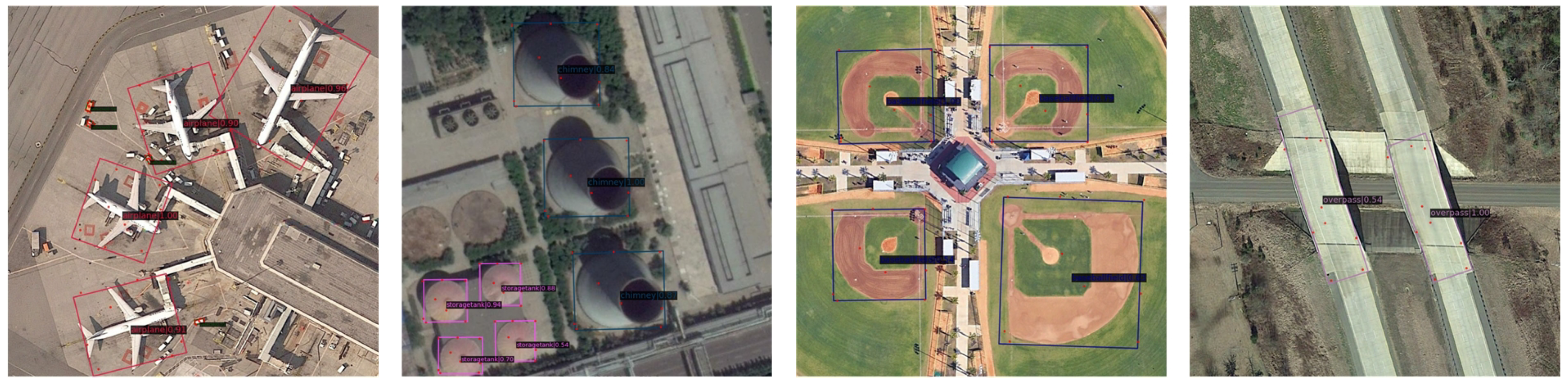
The object detection results obtained using the proposed SGR method are illustrated in Figure 7. As observed in the figure, the SGR method demonstrates its superior performance, characterized by precise distribution of sampling points, tightly fitted bounding box predictions, and accurate classification. These features collectively validate the effectiveness of the SGR approach in the realm of object detection.

4.5. Visualization of Results on Different Datasets

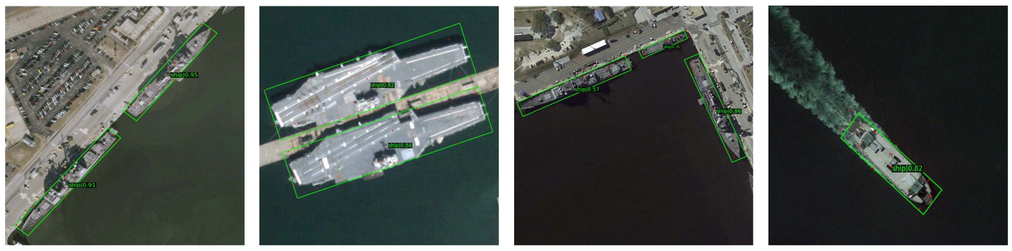
The results from the HRSC2016 dataset, illustrated in Figure 8, demonstrate our method’s capacity to generate precise and accurate detection boxes for ships. Such performance reflects the high precision of our method in detecting maritime objects, and underscores its capability to handle diverse orientations and sizes.

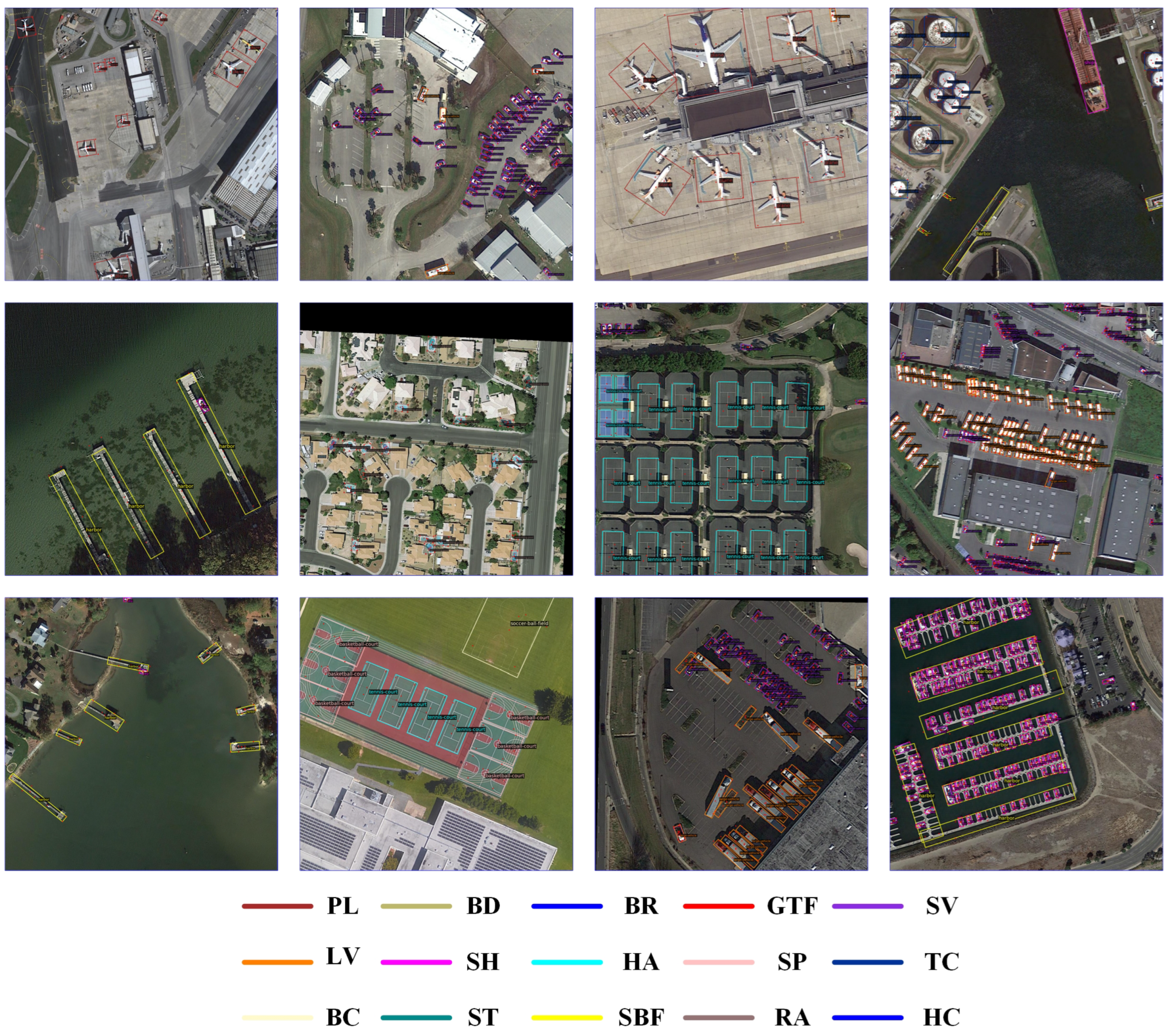
In the DIOR-R dataset, Figure 9 illustrates the effectiveness of our method in handling tasks involving a multitude of object categories. This ability to adeptly manage a diverse range of categories underscores the method’s robustness and confirms its suitability for complex and varied scenarios.

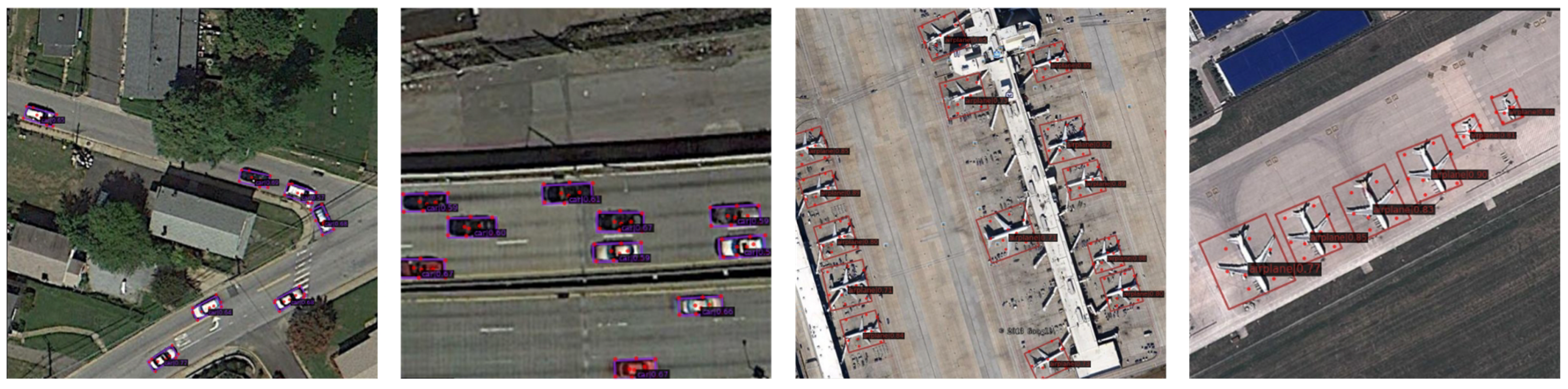
Figure 10 showcases the results on the UCAS-AOD dataset, where our method accurately detects a large number of vehicles and airplanes of different scales. This accuracy, despite the varying sizes and types of objects, underscores the effectiveness and reliability of our approach in diverse conditions.

5. Discussion

In this section, a discussion of the proposed method is provided, incorporating tables and images. The discussion encompasses the efficiency of the modules, the efficiency of the hyperparameters, and future directions.

5.1. Effectiveness of Saliency-Guided Methods

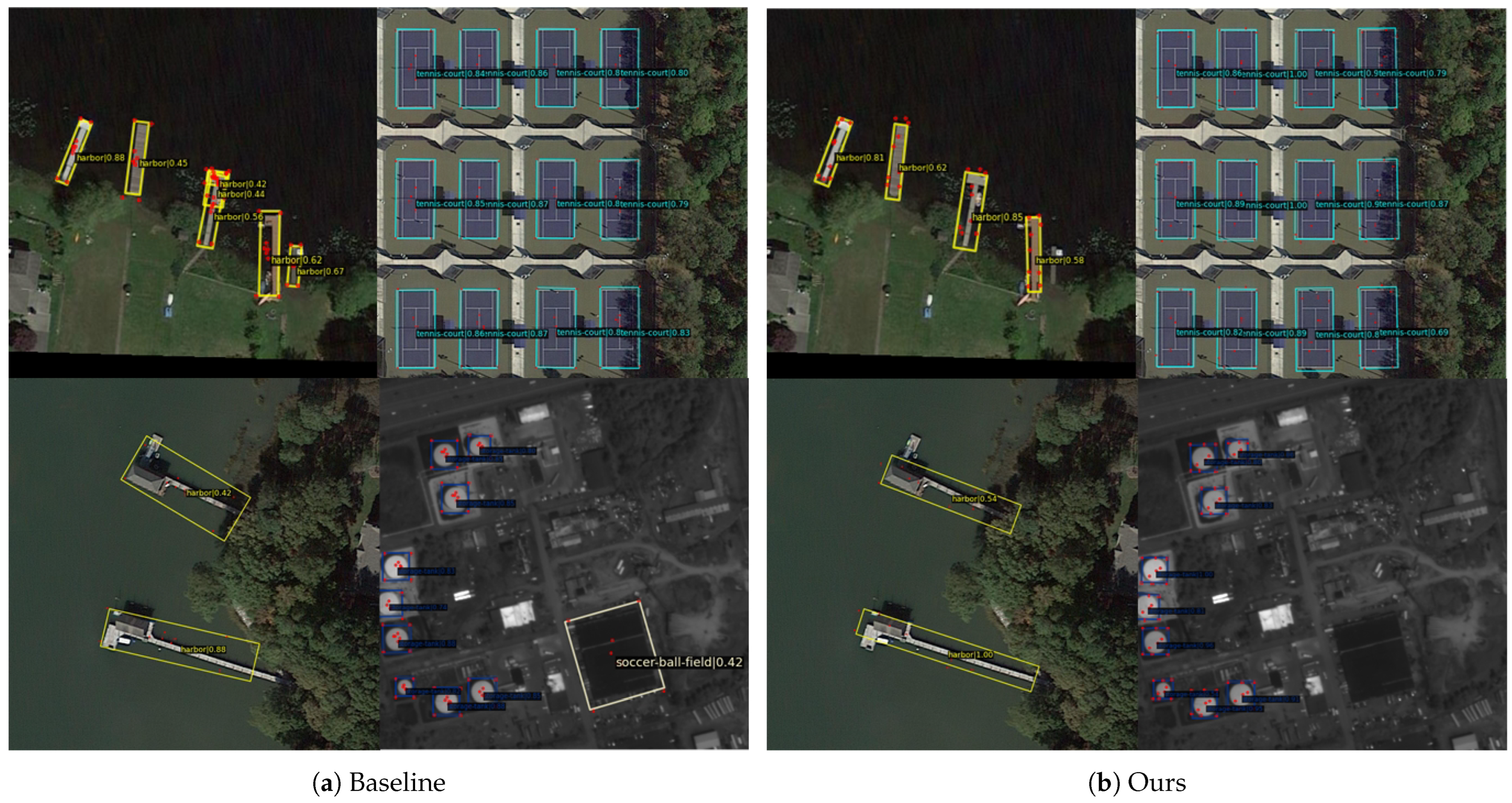
The positions of the sampling points before and after the improvement were compared, as depicted in Figure 11. In Figure 11a, it can be observed that a small portion of points are driven to the boundaries of the bounding boxes, while the majority of points are clustered around the center of the boxes, which represents the initial positions of the sampling points. This phenomenon occurs because the external points, guided by the convex IoU loss, tend to seek the boundaries. Their slight perturbations can greatly affect the value of the IoU loss, leading to larger gradients during the training optimization process. On the other hand, the internal points, which do not easily cause changes in the loss function, do not receive effective guidance and, thus, remain near their initial positions.

The effectiveness of the aforementioned sampling method can be attributed to the fact that a majority of the salient features of the target objects are indeed located at the center of the objects. This observation aligns with previous studies that hypothesized that sampling points following a two-dimensional Gaussian distribution can also yield satisfactory performance.

Point sampling, as a form of undersampling, should ideally focus on key areas to extract critical features. With this in mind, we implemented an SGR approach, which offers significant potential to enhance sampling efficiency by prioritizing areas of high importance in the data. This method allows for more targeted and effective feature extraction, thereby optimizing the use of the available data and improving overall model performance.

As previously shown in Table 1, our method has achieved significant improvement in detecting planes, harbors, helicopters, and other irregular objects. For these types of object, a considerable portion of the bounding box encompasses the background areas. The SGR method’s ability to precisely sample within these boxes effectively reduces noise interference, thereby enhancing detection performance for these irregularly shaped objects. The enhancement in detecting categories such as small vehicles, large vehicles, and swimming pools was comparatively modest. This limited improvement can largely be attributed to the inherent characteristics of these objects. They typically display homogeneous features within their respective bounding boxes, with a high degree of internal similarity, leading to less variability and distinction in their feature representations.

5.2. Assessing The Impact of SGR and DDA on Model Performance

In the ablation study detailed in

Table 5. Impact of SGR and DDA implementation in ablation study.

SGR	DDA	mAP (%)	$\Delta$
✕	✕	75.97	0
✕	✕	76.05 ${}^{†}$	+0.08 ${}^{†}$
✓	✕	76.24	+0.27
✓	✓	76.88	+0.91

The second row with † replaces the DCN in the classification branch of the baseline with a regular convolution.

, the first two rows reveal the impact of replacing the DCN in the RepPoints’ classification branch with traditional convolutions, which focus on features near the central region. This modification led to a slight increase in mAP, as shown in the second row, suggesting that traditional convolutions, with their stable spatial structures, are more effective in extracting features from central areas.

The third and fourth rows in Table 5 act as control experiments for the SGR method. The implementation of SGR resulted in a modest performance boost, with a mAP increase of 0.27%, as demonstrated in the fourth row. The finding underscores that merely applying the loss function to guide sampling points yields limited improvement. Such a directive approach, while enabling the upstream network to learn sampling in key areas spatially, does not necessarily ensure that the downstream predict head simultaneously comprehends this guidance. This discrepancy can lead to a potential misalignment between the spatial and feature domains.

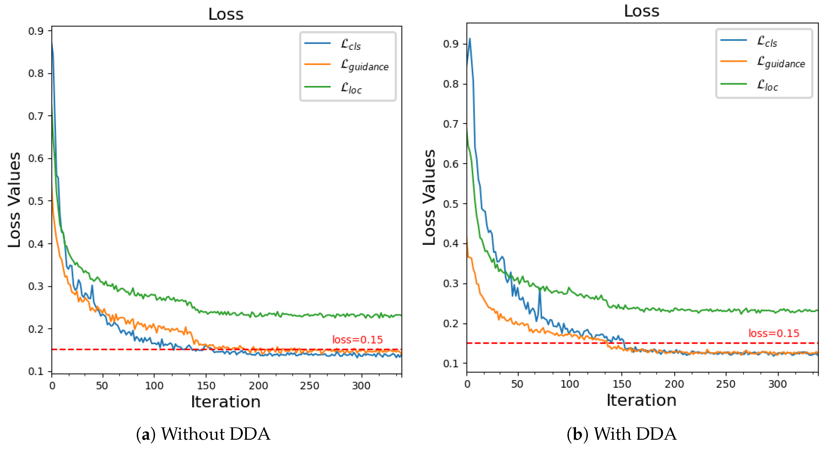
In contrast, the incorporation of DDA introduces posterior information predicted by the model to more effectively allocate sample labels. This method dynamically reconciles the balance between interpretability and model comprehension throughout the learning process, progressively fostering a synergistic alignment between the two domains. The loss curve depicted in Figure 6 during the training process provides evidence of further improvement in classification ability after the sampling pattern stabilizes upon applying DDA. This suggests an enhancement in the predict head’s capacity to comprehend feature representations.

5.3. Visual Interpretability Analysis of Alignment

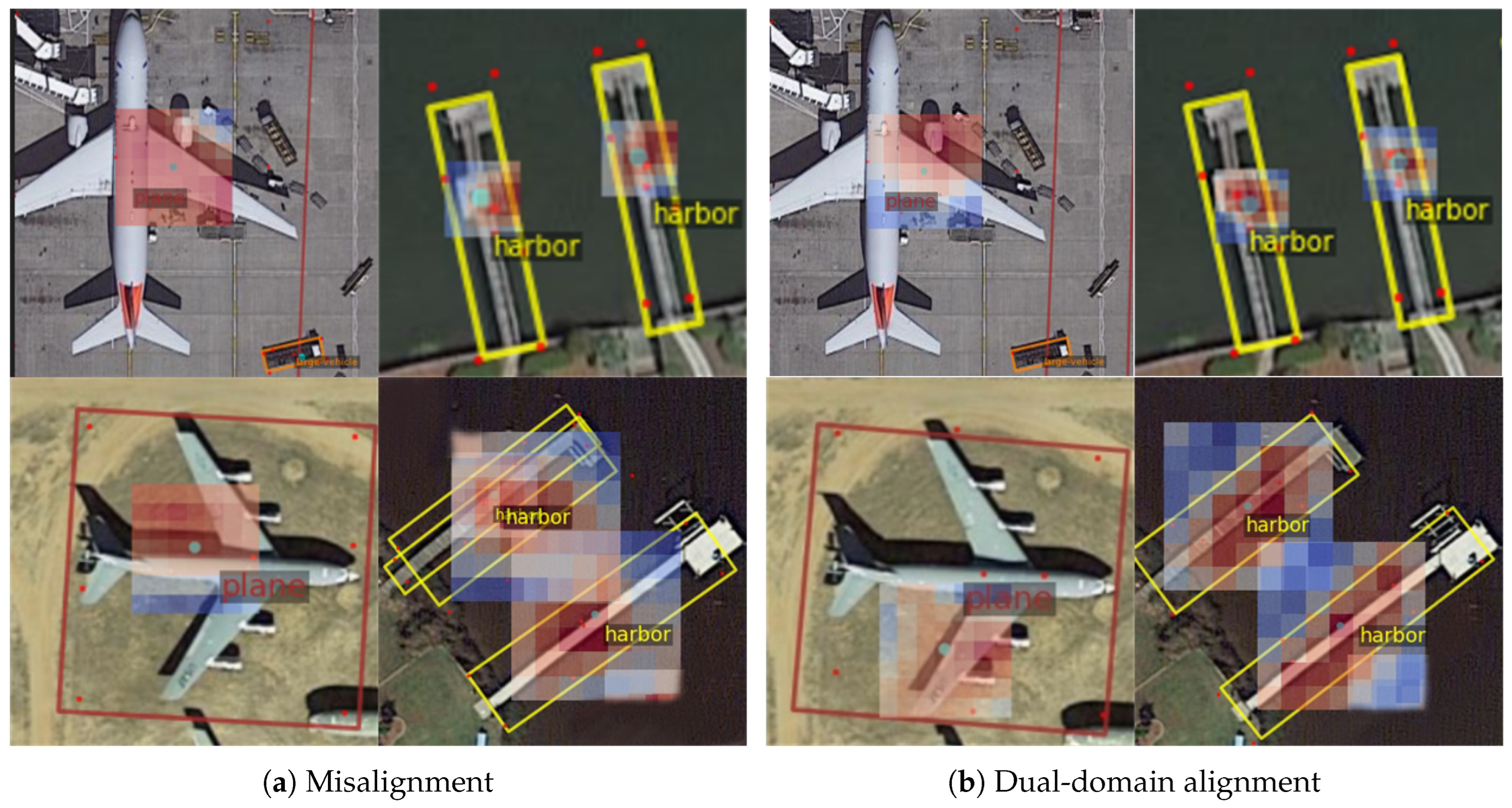
The visualization results leveraging the point local interpretable map method on the DOTA dataset are depicted in Figure 12. Instances of misalignment, as observed in experiments utilizing other methods, are showcased in Figure 12a. These include phenomena such as non-prominent activation in confused areas, background activation coupled with foreground suppression, and the occurrence of erroneous predictions. In stark contrast, Figure 12b displays the alignment between the spatial and feature domains. Notably, the activation regions near the airplane are concentrated around the engines and wings, indicating key areas of interest. Similarly, for the harbor, the activation points are more granular and precise. The direction of activation at the dock aligns with its spatial positioning, suggesting a high degree of accuracy in feature representation.

These observations imply that, from the perspective of the predict head, the distribution pattern of the sampling points appears rational and effective. The derived feature representations assist in reducing the ambiguity in classification tasks, thereby enhancing the model’s predictive accuracy. This contrast between the misaligned and aligned scenarios underscores the effectiveness of our approach in capturing and representing critical features in complex images.

5.4. Effectiveness of Hyperparameters

Within the proposed SGR framework, the loss and assignment measurements are pivotal in integrating saliency information into the guidance mechanism for sampling points. As outlined in Equations (6) and (10), the two key hyperparameters, ${\mathit{\lambda }}_3$ and ${\mathit{\mu }}_4$, are identified. A detailed discussion regarding the selection of these two hyperparameters follows below.

The hyperparameter ${\mathit{\lambda }}_3$ is used to balance ${\mathcal{L}}_{repulsion}$ with ${\mathcal{L}}_{loc}$ and ${\mathcal{L}}_{cls}$, representing the weight of the guidance constraint in the overall object detection task. As observed in

Table 6. Experimental evaluation of hyper-parameter ${\mathit{\lambda }}_3$ with ${\mathit{\lambda }}_1$ and ${\mathit{\lambda }}_2$ fixed at 1 and 0.375. The chosen values for ${\mathit{\lambda }}_3$ is highlighted in bold.

${\mathit{\lambda }}_3$	mAP (%)
0.10	75.93
0.15	76.74
0.20	76.88
0.25	76.18
0.30	75.66

, the model’s performance is quite sensitive to changes in ${\mathit{\lambda }}_3$, and it achieves better performance when ${\mathit{\lambda }}_3$ is around 0.2.

The hyperparameter ${\mathit{\mu }}_4$ influences the weight of prior spatial information in the matching process of the samples used for learning. The experimental results in

Table 7. Experimental evaluation of hyperparameter ${\mathit{\mu }}_4$ with ${\mathit{\mu }}_1$, ${\mathit{\mu }}_2$, and ${\mathit{\mu }}_3$ fixed at 1, 2, and 5. The chosen values for ${\mathit{\mu }}_4$ is highlighted in bold.

${\mu }_4$	1.0	1.5	2.0	2.5
mAP (%)	76.45	76.48	76.88	76.57

indicate that the model performs better when ${\mathit{\mu }}_4$ is around 2.0.

Apart from the hyperparameters discussed above, the other hyperparameters were selected based on experimental results and prior experience. They are coordinated and balanced with each other to optimize the model’s performance.

5.5. Future Directions Based on SGR

The discussions and experiments previously conducted, involving multiple challenging datasets, have highlighted the robust theoretical foundation and the practical effectiveness of the proposed SGR method. Although the efficacy of the SGR method has been established in this study, there remains a wealth of opportunities for further exploration within the framework of SGR. Future directions based on the SGR are discussed below.

Firstly, this work has already explored a path to interpretability, designing a visual, interpretable tool for evaluating model training effects. Moving forward, we plan to utilize interpretability tools to extract guiding information and to open up the model’s feature domain black box.

Secondly, considering model robustness and stability, we have adopted saliency maps as guiding information for the sampling points. This approach has validated the feasibility of guiding the DCN in learning sampling point distribution patterns. Future research may explore more fine-grained and interpretable distributions.

Lastly, we employed DDA to alleviate model misalignment in spatial and feature domains as our training strategy. In the future, we could enable the model to perform weighted sample selection autonomously, achieving dynamic attention and moving towards a more end-to-end approach.

In short, a validated and feasible framework for guiding the distribution patterns of DCN sampling points has been established. Building upon this established framework, there is considerable potential for further enhancements in the areas of interpretability and end-to-end processing.

6. Conclusions

In this work, we addressed the issue of inadequate guidance for sampling points during the feature representation stage in remote sensing object detection, a common limitation in previous DCN-based methods. We introduced a novel method SGR, which significantly enhances the capability of models to obtain accurate feature representations, thereby improving the performance of point-based object detectors. Furthermore, to mitigate the potential misalignment phenomena in the spatial and feature domains commonly encountered in model guiding processes, a dynamic dual-alignment assignment training strategy was proposed. This strategy effectively eases the optimization difficulty encountered during model training, allowing for the full realization of SGR’s capabilities. Additionally, an interpretable and visual tool was developed for qualitatively assessing the alignment in the spatial and feature domains. This tool can also be adapted for use with other point-based methods. Extensive experiments conducted across multiple datasets have validated the efficacy of our proposed method, achieving state-of-the-art performance.

Future research initiatives will expand upon the validated and feasible framework established in this study, aiming to refine the interpretability aspects within our guiding process. Furthermore, a systematic investigation into end-to-end detection methodologies is planned. These advancements are expected to enrich our comprehension and to bolster the performance of point-based detection techniques.

References

- Girshick, R. Fast r-cnn. In Proceedings of the IEEE International Conference on Computer Vision (ICCV), Santiago, Chile, 7–15 December 2015; pp. 1440–1448. [Google Scholar]
- Ren, S.; He, K.; Girshick, R.; Sun, J. Faster R-CNN: Towards Real-Time Object Detection with Region Proposal Networks. IEEE Trans. Pattern Anal. Mach. Intell. 2016, 39, 1137–1149. [Google Scholar] [CrossRef] [PubMed]
- Zhao, Z.Q.; Zheng, P.; Xu, S.t.; Wu, X. Object detection with deep learning: A review. IEEE Trans. Neural Netw. Learn. Syst. 2019, 30, 3212–3232. [Google Scholar] [CrossRef] [PubMed]
- Wang, Y.; Bashir, S.M.A.; Khan, M.; Ullah, Q.; Wang, R.; Song, Y.L.; Guo, Z.; Niu, Y.L. Remote sensing image super-resolution and object detection: Benchmark and state of the art. Expert Syst. Appl. 2022, 197, 19. [Google Scholar] [CrossRef]
- Dong, Z.; Wang, M.; Wang, Y.; Liu, Y.; Feng, Y.; Xu, W. Multi-oriented object detection in high-resolution remote sensing imagery based on convolutional neural networks with adaptive object orientation features. Remote Sens. 2022, 14, 950. [Google Scholar] [CrossRef]
- He, K.; Gkioxari, G.; Dollár, P.; Girshick, R. Mask r-cnn. In Proceedings of the IEEE International Conference on Computer Vision (ICCV), Santiago, Chile, 7–15 December 2015; pp. 2961–2969. [Google Scholar]
- Xie, X.X.; Cheng, G.; Wang, J.B.; Yao, X.W.; Han, J.W. Oriented R-CNN for Object Detection. In Proceedings of the 18th IEEE/CVF International Conference on Computer Vision (ICCV), New York, NY, USA, 10–17 October 2021; pp. 3500–3509. [Google Scholar] [CrossRef]
- Dai, J.; Qi, H.; Xiong, Y.; Li, Y.; Zhang, G.; Hu, H.; Wei, Y. Deformable convolutional networks. In Proceedings of the IEEE international conference on computer vision, Venice, Italy, 22–29 October 2017; pp. 764–773. [Google Scholar]
- Zhu, X.Z.; Hu, H.; Lin, S.; Dai, J.F.; Soc, I.C. Deformable ConvNets v2: More Deformable, Better Results. In Proceedings of the IEEE/CVF Conference on Computer Vision and Pattern Recognition (CVPR), New York, NY, USA, 27–28 March 2019; pp. 9300–9308. [Google Scholar] [CrossRef]
- Han, J.M.; Ding, J.; Li, J.; Xia, G.S. Align Deep Features for Oriented Object Detection. IEEE Trans. Geosci. Remote Sens. 2022, 60, 11. [Google Scholar] [CrossRef]
- Cheng, B.; Wei, Y.; Shi, H.; Feris, R.; Xiong, J.; Huang, T. Revisiting rcnn: On awakening the classification power of faster rcnn. In Proceedings of the European Conference on Computer Vision (ECCV), Munich, Germany, 8–14 September 2018; pp. 453–468. [Google Scholar]
- Ding, J.; Xue, N.; Long, Y.; Xia, G.S.; Lu, Q.K.; Soc, I.C. Learning RoI Transformer for Oriented Object Detection in Aerial Images. In Proceedings of the 32nd IEEE/CVF Conference on Computer Vision and Pattern Recognition (CVPR), Long Beach, CA, USA, 15–20 June 2019; pp. 2844–2853. [Google Scholar]
- Zhou, Q.; Yu, C.H. Point RCNN: An Angle-Free Framework for Rotated Object Detection. Remote Sens. 2022, 14, 23. [Google Scholar] [CrossRef]
- Hou, L.P.; Lu, K.; Xue, J.; Li, Y.Q.; Assoc Advancement Artificial, I. Shape-Adaptive Selection and Measurement for Oriented Object Detection. In Proceedings of the 36th AAAI Conference on Artificial Intelligence/34th Conference on Innovative Applications of Artificial Intelligence/12th Symposium on Educational Advances in Artificial Intelligence, Palo Alto, CA, USA, 23–25 January 2022; pp. 923–932. [Google Scholar]
- Zhang, T.; Sun, X.; Zhuang, L.; Dong, X.; Sha, J.; Zhang, B.; Zheng, K. AFRE-Net: Adaptive Feature Representation Enhancement for Arbitrary Oriented Object Detection. Remote Sens. 2023, 15, 4965. [Google Scholar] [CrossRef]
- Hou, L.P.; Lu, K.; Yang, X.; Li, Y.Q.; Xue, J. G-Rep: Gaussian Representation for Arbitrary-Oriented Object Detection. Remote Sens. 2023, 15, 21. [Google Scholar] [CrossRef]
- Xu, C.; Ding, J.; Wang, J.; Yang, W.; Yu, H.; Yu, L.; Xia, G.S. Dynamic Coarse-to-Fine Learning for Oriented Tiny Object Detection. In Proceedings of the IEEE/CVF Conference on Computer Vision and Pattern Recognition, Vancouver, BC, Canada, 17–24 June 2023; pp. 7318–7328. [Google Scholar]
- Yang, Z.; Liu, S.H.; Hu, H.; Wang, L.; Lin, S. RepPoints: Point Set Representation for Object Detection. In Proceedings of the IEEE/CVF International Conference on Computer Vision (ICCV), New York, NY, USA, 27–28 March 2019; pp. 9656–9665. [Google Scholar] [CrossRef]
- Chen, Y.; Zhang, Z.; Cao, Y.; Wang, L.; Lin, S.; Hu, H. Reppoints v2: Verification meets regression for object detection. Adv. Neural Inf. Process. Syst. 2020, 33, 5621–5631. [Google Scholar]
- Li, W.T.; Chen, Y.J.; Hu, K.X.; Zhu, J.K. Oriented RepPoints for Aerial Object Detection. In Proceedings of the IEEE/CVF Conference on Computer Vision and Pattern Recognition (CVPR), New Orleans, LA, USA, 18–24 June 2022; pp. 1819–1828. [Google Scholar] [CrossRef]
- Gabriel, I. Artificial intelligence, values, and alignment. Minds Mach. 2020, 30, 411–437. [Google Scholar] [CrossRef]
- Cheng, G.; Yao, Y.; Li, S.; Li, K.; Xie, X.; Wang, J.; Yao, X.; Han, J. Dual-aligned oriented detector. IEEE Trans. Geosci. Remote Sens. 2022, 60, 1–11. [Google Scholar] [CrossRef]
- Xia, G.S.; Bai, X.; Ding, J.; Zhu, Z.; Belongie, S.; Luo, J.; Datcu, M.; Pelillo, M.; Zhang, L. DOTA: A large-scale dataset for object detection in aerial images. In Proceedings of the IEEE Conference on Computer Vision and Pattern Recognition, Salt Lake City, UT, USA, 18–23 June 2018; pp. 3974–3983. [Google Scholar]
- Liu, Z.; Yuan, L.; Weng, L.; Yang, Y. A high resolution optical satellite image dataset for ship recognition and some new baselines. In International Conference on Pattern Recognition Applications and Methods; SciTePress: Setúbal, Portugal, 2017; Volume 2, pp. 324–331. [Google Scholar]
- Cheng, G.; Wang, J.; Li, K.; Xie, X.; Lang, C.; Yao, Y.; Han, J. Anchor-free oriented proposal generator for object detection. IEEE Trans. Geosci. Remote Sens. 2022, 60, 1–11. [Google Scholar] [CrossRef]
- Zhu, H.; Chen, X.; Dai, W.; Fu, K.; Ye, Q.; Jiao, J. Orientation robust object detection in aerial images using deep convolutional neural network. In Proceedings of the 2015 IEEE International Conference on Image Processing (ICIP), Quebec City, QC, Canada, 27–30 September 2015; pp. 3735–3739. [Google Scholar]
- Li, Y.; Li, Z.; Ye, F.; Jiang, T. Reppoints-Based Multi-Scale Task Enhancement Network and Sample Assignment Method For Oriented Object Detection. IEEE Geosci. Remote Sens. Lett. 2023, 20, 6009305. [Google Scholar]
- Le, T.V.; Van, H.N.N.; Bui, D.C.; Vo, P.; Vo, N.D.; Nguyen, K. Empirical study of reppoints representation for object detection in aerial images. In Proceedings of the 2022 IEEE Ninth International Conference on Communications and Electronics (ICCE), Nha Trang, Vietnam, 27–29 July 2022; pp. 337–342. [Google Scholar]
- Xu, C.; Su, H.; Gao, L.; Wu, J.; Yan, W.; Li, J. Feature Aligned Ship Detection Based on RepPoints in SAR Images. In International Forum on Digital TV and Wireless Multimedia Communications; Springer: Singapore, 2021; pp. 71–82. [Google Scholar]
- Gao, L.; Gao, H.; Wang, Y.; Liu, D.; Momanyi, B.M. Center-Ness and Repulsion: Constraints to Improve Remote Sensing Object Detection via RepPoints. Remote Sens. 2023, 15, 1479. [Google Scholar] [CrossRef]
- Yang, X.; Yan, J. Arbitrary-oriented object detection with circular smooth label. In Proceedings of the Computer Vision–ECCV 2020: 16th European Conference, Proceedings, Part VIII 16, Glasgow, UK, 23–28 August 2020; pp. 677–694. [Google Scholar]
- You, Y.; Ran, B.; Meng, G.; Li, Z.; Liu, F.; Li, Z. OPD-Net: Prow detection based on feature enhancement and improved regression model in optical remote sensing imagery. IEEE Trans. Geosci. Remote Sens. 2020, 59, 6121–6137. [Google Scholar] [CrossRef]
- Yang, X.; Yan, J.; Ming, Q.; Wang, W.; Zhang, X.; Tian, Q. Rethinking rotated object detection with gaussian wasserstein distance loss. In Proceedings of the International Conference on Machine Learning, PMLR, Virtual Event, 18–24 July 2021; pp. 11830–11841. [Google Scholar]
- Yang, X.; Hou, L.; Zhou, Y.; Wang, W.; Yan, J. Dense label encoding for boundary discontinuity free rotation detection. In Proceedings of the IEEE/CVF Conference on Computer Vision and Pattern Recognition, Seattle, WA, USA, 13–19 June 2020; pp. 15819–15829. [Google Scholar]
- Yu, Y.; Da, F. Phase-shifting coder: Predicting accurate orientation in oriented object detection. In Proceedings of the IEEE/CVF Conference on Computer Vision and Pattern Recognition, Nashville, TN, USA, 20–25 June 2021; pp. 13354–13363. [Google Scholar]
- Zhang, S.; Chi, C.; Yao, Y.; Lei, Z.; Li, S.Z. Bridging the gap between anchor-based and anchor-free detection via adaptive training sample selection. In Proceedings of the IEEE/CVF Conference on Computer Vision and Pattern Recognition, Long Beach, CA, USA, 15–20 June 2019; pp. 9759–9768. [Google Scholar]
- Ming, Q.; Zhou, Z.; Miao, L.; Zhang, H.; Li, L. Dynamic anchor learning for arbitrary-oriented object detection. In Proceedings of the AAAI Conference on Artificial Intelligence, New York, NY, USA, 7–12 February 2020; Volume 35, pp. 2355–2363. [Google Scholar]
- Wang, J.; Song, L.; Li, Z.; Sun, H.; Sun, J.; Zheng, N. End-to-end object detection with fully convolutional network. In Proceedings of the IEEE/CVF Conference on Computer Vision and Pattern Recognition, Seattle, WA, USA, 13–19 June 2020; pp. 15849–15858. [Google Scholar]
- Ming, Q.; Miao, L.J.; Zhou, Z.Q.; Yang, X.; Dong, Y.P. Optimization for Arbitrary-Oriented Object Detection via Representation Invariance Loss. IEEE Geosci. Remote Sens. Lett. 2022, 19, 5. [Google Scholar] [CrossRef]
- Zhang, S.; Wang, X.; Wang, J.; Pang, J.; Lyu, C.; Zhang, W.; Luo, P.; Chen, K. Dense Distinct Query for End-to-End Object Detection. In Proceedings of the IEEE/CVF Conference on Computer Vision and Pattern Recognition, Vancouver, BC, Canada, 17–24 June 2023; pp. 7329–7338. [Google Scholar]
- Hou, X.; Zhang, L. Saliency detection: A spectral residual approach. In Proceedings of the 2007 IEEE Conference on Computer Vision and Pattern Recognition, Minneapolis, MN, USA, 17–22 June 2007; pp. 1–8. [Google Scholar]
- Padilla, R.; Netto, S.L.; Da Silva, E.A. A survey on performance metrics for object-detection algorithms. In Proceedings of the 2020 International Conference on Systems, Signals and Image Processing (IWSSIP), Niteroi, Brazil, 1–3 July 2020; pp. 237–242. [Google Scholar]
- Lin, T.Y.; Goyal, P.; Girshick, R.; He, K.; Dollár, P. Focal loss for dense object detection. In Proceedings of the IEEE International Conference on Computer Vision, Venice, Italy, 22–29 October 2017; pp. 2980–2988. [Google Scholar]
- Qian, W.; Yang, X.; Peng, S.; Yan, J.; Guo, Y. Learning modulated loss for rotated object detection. In Proceedings of the AAAI Conference on Aartificial Intelligence, Washington, DC, USA, 7–14 February 2023; Volume 35, pp. 2458–2466. [Google Scholar]
- Yang, X.; Yan, J.C.; Feng, Z.M.; He, T. R3Det: Refined Single-Stage Detector with Feature Refinement for Rotating Object. In Proceedings of the 35th AAAI Conference on Artificial Intelligence/33rd Conference on Innovative Applications of Artificial Intelligence/11th Symposium on Educational Advances in Artificial Intelligence, Palo Alto, CA, USA, 23–25 January 2021; Volume 35, pp. 3163–3171. [Google Scholar]
- Zhang, G.; Lu, S.; Zhang, W. CAD-Net: A context-aware detection network for objects in remote sensing imagery. IEEE Trans. Geosci. Remote Sens. 2019, 57, 10015–10024. [Google Scholar] [CrossRef]
- Yang, X.; Yang, J.; Yan, J.; Zhang, Y.; Zhang, T.; Guo, Z.; Sun, X.; Fu, K. Scrdet: Towards more robust detection for small, cluttered and rotated objects. In Proceedings of the IEEE/CVF international Conference on Computer Vision, Salt Lake City, UT, USA, 18–23 June 2018; pp. 8232–8241. [Google Scholar]
- Li, C.; Xu, C.; Cui, Z.; Wang, D.; Zhang, T.; Yang, J. Feature-attentioned object detection in remote sensing imagery. In Proceedings of the 2019 IEEE international Conference on Image Processing (ICIP), Taipei, Taiwan, 22–25 September 2019; pp. 3886–3890. [Google Scholar]
- Xu, Y.; Fu, M.; Wang, Q.; Wang, Y.; Chen, K.; Xia, G.S.; Bai, X. Gliding vertex on the horizontal bounding box for multi-oriented object detection. IEEE Trans. Pattern Anal. Mach. Intell. 2020, 43, 1452–1459. [Google Scholar] [CrossRef]
- Wang, J.; Ding, J.; Guo, H.; Cheng, W.; Pan, T.; Yang, W. Mask OBB: A semantic attention-based mask oriented bounding box representation for multi-category object detection in aerial images. Remote Sens. 2019, 11, 2930. [Google Scholar] [CrossRef]
- Wang, J.; Yang, W.; Li, H.C.; Zhang, H.; Xia, G.S. Learning center probability map for detecting objects in aerial images. IEEE Trans. Geosci. Remote Sens. 2020, 59, 4307–4323. [Google Scholar] [CrossRef]
- Han, J.; Ding, J.; Xue, N.; Xia, G.S. Redet: A rotation-equivariant detector for aerial object detection. In Proceedings of the IEEE/CVF Conference on Computer Vision and Pattern Recognition, Nashville, TN, USA, 20–25 June 2021; pp. 2786–2795. [Google Scholar]
- Zhou, X.; Wang, D.; Krähenbühl, P. Objects as points. arXiv 2019, arXiv:1904.07850. [Google Scholar]
- Chen, Z.; Chen, K.; Lin, W.; See, J.; Yu, H.; Ke, Y.; Yang, C. Piou loss: Towards accurate oriented object detection in complex environments. In Proceedings of the Computer Vision–ECCV 2020: 16th European Conference, Glasgow, UK, 23–28 August 2020; Part V 16. pp. 195–211. [Google Scholar]
- Wei, H.; Zhang, Y.; Chang, Z.; Li, H.; Wang, H.; Sun, X. Oriented objects as pairs of middle lines. ISPRS J. Photogramm. Remote Sens. 2020, 169, 268–279. [Google Scholar] [CrossRef]
- Yang, J.; Liu, Q.; Zhang, K. Stacked hourglass network for robust facial landmark localisation. In Proceedings of the IEEE Conference on Computer Vision and Pattern Recognition Workshops, Honolulu, HI, USA, 21–26 July 2017; pp. 79–87. [Google Scholar]
- Pan, X.; Ren, Y.; Sheng, K.; Dong, W.; Yuan, H.; Guo, X.; Ma, C.; Xu, C. Dynamic refinement network for oriented and densely packed object detection. In Proceedings of the IEEE/CVF Conference on Computer Vision and Pattern Recognition, Seattle, WA, USA, 13–19 June 2020; pp. 11207–11216. [Google Scholar]
- Guo, Z.; Liu, C.; Zhang, X.; Jiao, J.; Ji, X.; Ye, Q. Beyond bounding-box: Convex-hull feature adaptation for oriented and densely packed object detection. In Proceedings of the IEEE/CVF Conference on Computer Vision and Pattern Recognition, Nashville, TN, USA, 20–25 June 2021; pp. 8792–8801. [Google Scholar]
- Huang, Z.; Li, W.; Xia, X.G.; Tao, R. A general Gaussian heatmap label assignment for arbitrary-oriented object detection. IEEE Trans. Image Process. 2022, 31, 1895–1910. [Google Scholar] [CrossRef] [PubMed]
- Redmon, J.; Farhadi, A. Yolov3: An incremental improvement. arXiv 2018, arXiv:1804.02767. [Google Scholar]
Figure 1.
Various distribution patterns of sampling points. The patterns depicted in (a,b) represent fixed distributions. In (c), the sampling points are guided to a limited extent, focusing on boundary detection, while (d) demonstrates the SGR method, focusing on key regions.
Figure 2.
Different methods for obtaining feature representation. (a) Traditional convolution methods sample from an axis-aligned square region to obtain a pixel in the feature map. (b) RoI-based methods derive a fixed feature representation from a region of interest. (c) Deformable convolution can adaptively obtain a pixel in the feature map based on the offset in the feature representation.
Figure 3.
The overall pipeline of our method. Our method, based on the RepPoints, flexibly obtains feature representation through the DCN structure.
Figure 4.
Illustration of learning process. Sampling points learn to identify salient features and boundaries.
Figure 5.
Procession of DDA. The main pipeline is depicted to the left of the black dashed line. The measurement matrix is calculated based on the defined measurements function and subsequently fed into the Hungarian algorithm for global minimization matching. All matching measurements are non-positive numbers, with smaller measurements indicating a better match between the sample and the ground truth. The integration of the Hungarian algorithm and the measurement matrix enables dynamic consideration of diverse information, thereby providing high-quality labels for the samples.
Figure 6.
Comparative analysis of loss curves with and without the application of DDA.
Figure 7.
Visualization of the detection results of our method on the DOTA dataset is provided. The different colors of the boxes represent different categories. The red points are the key points predicted by the model, and subsequent localization and classification are based on the feature representation sampled from these points.
Figure 8.
Results on the HRSC2016 dataset, showcasing the detection of ships, which illustrates the adaptability of our method to various orientations and sizes.
Figure 9.
Results on the DIOR-R dataset, displaying the detection of multiple object categories, demonstrating the robustness of our method.
Figure 10.
Results on the UCAS-AOD dataset, presenting the comprehensive detection of airplanes and cars.
Figure 11.
Comparative analysis of baseline and proposed saliency-guided methods: Our method demonstrates notable improvements, characterized by the suppression of false alarms, a more rational distribution of sampling points, precise bounding box regression, and increased confidence in classifications.
Figure 12.
Assessing the impact of DDA by point local interpretable map. The right-side picture illustrates more refined and logically patterned activation than the left-side picture. Blue points denote variable sampling points. The heat map illustrates classification score changes upon the movement of these points in the grid area, with red for increase and blue for decrease.