
The Study of Internal Gravity Waves in the Earth’s Atmosphere by Radio Occultations: A Review

1
A.M. Obukhov Institute of Atmospheric Physics, Russian Academy of Sciences, Pyzhevsky Per. 3, Moscow 119017, Russia
2
Hydrometcenter of Russia, Bolshoy Predtechensky Per. 13, Building 1, Moscow 123376, Russia
*
Author to whom correspondence should be addressed.
Remote Sens. 2024, 16(2), 221; https://doi.org/10.3390/rs16020221
Submission received: 27 November 2023
/
Revised: 30 December 2023
/
Accepted: 3 January 2024
/
Published: 5 January 2024
(This article belongs to the Section Satellite Missions for Earth and Planetary Exploration)
Abstract
:Internal gravity waves (IGWs) in the middle atmosphere are the main source of mesoscale fluctuations of wind and temperature. The parameterization of IGWs and study of their climatology is necessary for the development of global atmospheric circulation models. In this review, we focus on the application of Radio Occultation (RO) observations for the retrieval of IGW parameters. (1) The simplest approach employs the retrieved temperature profiles. It is based on the fact that IGWs are highly anisotropic structures and can be accurately retrieved by RO. The basic assumption is that all the temperature fluctuations are caused by IGWs. The smoothed background temperature profile defines the the Brunt–Väisälä frequency, which, together with the temperature fluctuations, defines the IGW specific potential energy. Many studies have derived the distribution and climatology of potential energy, which is one of the most important characteristics of IGWs. (2) More detailed analysis of the temperature profiles is based on the derivation of the temperature fluctuation spectra. For saturated IGWs, the spectra must obey the power law with an exponent of . Such spectra are obtained by using Wave Optical (WO) processing. (3) More advanced analysis employs space–frequency analysis. It is based on phase-sensitive techniques like cross S- or wavelet transforms in order to identify propagating IGWs. (4) Another direction is the IGW parameter estimate from separate temperature profiles applying the stability condition in terms of the Richardson number. In this framework, a necessary condition is formulated that defines whether or not the temperature fluctuations can be related to IGW events. The temperature profile retrieval involves integral transforms and filtering that constitute the observation filter. (5) A simpler filter is implemented by the analysis of the RO amplitude fluctuation spectra, based on the diffraction theory in the framework of the phase screen and weak fluctuation approximations. The two spectral parameters, the external scale and the structural characteristic, define the specific potential energy. This approach allows the derivation of the spacial and seasonal distributions of IGW activity. We conclude that the success of IGW study by RO is stimulated by a large number of RO observations and advanced techniques based on Fourier and space–time analysis, physical equations describing IGWs, and diffraction theory.
1. Introduction
Internal gravity waves (IGWs) in the middle atmosphere are the main source of mesoscale fluctuations of wind and temperature. The vertical scales of IGWs vary from several kilometers to hundreds of meters, and the periods vary from 5 min to 10 h. They play a significant role in the energy exchange and global circulation of the atmosphere, the generation of turbulence, and mixing [1]. The parameterization of IGWs and the study of the spatial and seasonal distributions of their activity are crucial for the development of global atmospheric circulation models. IGW observations are based on the measurements of temperature and wind fluctuations performed by radiosondes at globally distributed ground stations [2,3,4], by radars [5,6], and by aircrafts [7,8]. Satellite observations, with their global spatio-temporal coverage, provide a powerful means for the study of IGWs. As examples, we can mention limb spectrometers [9,10] and stellar occultations [11,12,13,14].
The Radio Occultation (RO) sounding of the Earth’s atmosphere [15,16,17,18,19,20,21,22] employs the high-precision signals of the Global Navigation Satellite Systems (GNSSs), received by constellations of space-borne receivers. RO observations attracted the attention of the IGW community after the first successful proof-of-concept experiments. The following characteristics of RO make it suitable for monitoring IGWs: (1) global coverage; (2) an increasing number of sounders; (3) all-weather capability; (4) insensitivity to clouds; (5) insensitivity to small-scale inhomogeneities like the Kolmogorov turbulence; (6) a deeper penetration due to smaller amplitude scintillation as compared to stellar occultations; (7) a sub-Fresnel vertical resolution due to the application of wave optical (WO) processing algorithms utilizing the measurements of both amplitude and phase [23,24,25]; (8) IGWs are anisotropic inhomogeneities, with the horizontal-to-vertical scale ratio achieving values in the hundreds, while RO is primarily sensitive to this type of structure. Some of these advantages, like (5), (6), and (7), are based on the use of radio frequencies.
An IGW is a complicated physical process covering a wide range of scales and interacting with other atmospheric structures. This makes the interpretation of the observational data in terms of IGW parameters a difficult problem. In this review, we concentrate on the derivation of IGW parameters from RO observations and discuss different approaches.
The simplest approach uses the retrieved temperature profiles. After subtracting the large-scale background, the remaining perturbation is treated as linked to IGWs. This technique was applied to the observations provided by different RO missions [26,27,28,29,30,31,32,33,34,35,36,37]. The seasonal, latitudinal, longitudinal, and vertical variations of specific potential energy were derived and analyzed. Precaution was taken regarding the Inertial Instability (II) that in some cases may cause large temperature fluctuations masquerading as IGWs.
The temperature fluctuation spectra provide more detailed information, as compared to the derivation of the IGW specific potential energy from the fluctuation magnitude. The spectral slope is dictated by the “universal” IGW spectrum and can be used for IGW identification. This direction was presented in [38,39,40,41,42]. The question of how the spectra are influenced by the hydrostatic balance assumption was posed.
The aforementioned studies used large arrays of RO events as if they were independent. If fact, propagating IGWs with their large horizontal scales result in correlation between different events. This fact is utilized by space–frequency analysis based on the S-transform and continuous wavelet transform (CWT) [43,44,45,46,47,48]. Space–frequency analysis localizes spatial frequencies by linking them to spatial coordinates. This technique is capable of revealing IGW patterns in the 3D temperature field, using the dispersion relation between the vertical and horizontal space frequencies. Its other application is Momentum Flux (MF) estimation [46,49]. Nath et al. [50] used the symmetry properties of the spatial spectra of temperature fluctuations to distinguish between IGWs and different types of planetary waves.
Another approach to the identification of IGWs [51,52] uses the stability condition formulated in terms of the Richardson number. It allows the derivation of the intrinsic frequency, the intrinsic horizontal phase speed, the vertical phase speed, and the amplitude of the horizontal velocity perturbation from single temperature profiles.
Temperature profile retrieval involves integral transforms and filtering, which constitute the observation filter. A simpler filter is implemented by the analysis of the RO amplitude fluctuation spectra, based on the diffraction theory, previously developed for the derivation of IGW parameters from stellar occultations [53,54,55]. Using the linear theory based on the phase screen and weak fluctuation approximations, simple expressions are derived for the amplitude fluctuation spectra that link them to the IGW temperature fluctuation spectra. By fitting the theoretical spectra to the observed ones, it is possible to reconstruct the parameters of the IGW spectra. The two spectral parameters, the external scale and the structural characteristic, define the specific potential energy. This approach allows the derivation of the spacial and seasonal distributions of IGW activity.
The paper is organized as follows. Section 2 contains the basic physical relations describing the physics of IGWs. Section 3 is the main part of the review, describing different methods of studying IGWs from RO observations. It contains the following subsections: Section 3.1 describes studies based on the retrieved temperature profiles. Section 3.2 describes the reconstruction of the temperature fluctuation spectra. Section 3.3 describes the application of space–frequency analysis techniques to identify IGWs and to derive their vertical and horizontal scales. Section 3.4 describes the retrieval of IGW parameters from single temperature profiles. Section 3.5 discusses studies based on the application of the diffraction theory to the derivation of IGW parameters from the amplitude fluctuation spectra. In Section 4, we offer our conclusions.
2. The Properties of Internal Gravity Waves
IGWs in the atmosphere are oscillating departures from the stably stratified background state, the buoyancy acting as the restoring force [1]. The description of IGWs is obtained in the approximation of small plane-wave perturbations of x, y, and z components of wind velocity, , , and , respectively, and relative perturbations of the potential temperature , pressure , and density , where a prime denotes the perturbation, and a bar denotes the background value. The plane wave has the following form:
Here, are the components of the spatial frequency vector , is the temporal frequency, and H is the characteristic vertical scale of the atmosphere:
The typical value of H is about 7 km.
The dispersion relation is obtained from the system of the fluid dynamics equations linearized with respect to small perturbations. To this end, the Coriolis parameter f and the Brunt–Väisälä (buoyancy) frequency are defined as follows:
where is the angular velocity of the Earth’s rotation, is the geodetic latitude, g is the gravity acceleration, is the ratio of the isobaric and isochoric specific heat capacities for dry air, and Rd = 287.06 J K−1 kg−1 is the gas constant for dry air. Excluding the acoustic waves, one arrives at the dispersion relation for IGWs:
where the intrinsic frequency related to the coordinate frame moving horizontally with the air mass, and the horizontal spatial frequency .
Formally, can be both real and imaginary, the latter case corresponding to so-called inhomogeneous waves, which exponentially increase/decrease the amplitude along some directions. We, however, require that in order to consider conventional propagating waves. Then, from (4), it follows that cannot equal zero, i.e., IGWs cannot propagate purely vertically, which is important from the view point of RO inversion, where the assumption of the locally spherically layered structure plays a key role. Another conclusion is that the intrinsic frequency has both lower and upper limits: .
Numerous mechanisms are responsible for the generation of IGWs: topographic generation, convective generation, shear generation, geostrophic adjustment, and nonlinear wave–wave interaction [1]. To us, it is important that IGWs form a random ensemble that can be statistically described by the spectral density. The typical model of the vertical 1D spectrum of a saturated IGW [1,56,57] has the following form:
where is the normalization constant; s is the power exponent for low frequencies; is the power index for high frequencies; and is the external vertical wavenumber, corresponding to the external scale . The rightmost expression is the high-frequency asymptotic. The typical value of for a saturated IGW is 3.
The following 3D anisotropic spectrum, which generalizes the 1D spectrum [11,12,58], was used in [13] for the study of IGWs:
where is the structure constant, is the anisotropy coefficient, and is the power index. This spectrum can be multiplied with a function characterizing the spectrum decay at large wavenumbers exceeding the internal one corresponding to the internal scale . However, RO observations are insensitive to , and we will not use it in this paper. The 1D spectrum is obtained from the 3D spectrum by integration over , and . The typical value of is, therefore, 5.
The model spectrum with constant anisotropy (6) gives the same power index for the dependence from the horizontal wavelength, which does not agree with experimental data [1] that indicate a typical power index of . More advanced models with a variable anisotropy were introduced by Gurvich [59], Gurvich and Chunchuzov [60], the latter demonstrating good agreement with the observations. On the other hand, as shown by Gurvich and Brekhovskikh [58], in limb sounding geometry, the values of anisotropy exceeding a threshold of about 30 are indistinguishable. The horizontal wavelength of IGWs ranges from tens to thousands of kilometers, while the horizontal resolution of limb sounding is hundreds of kilometers [61]. Therefore, RO observations are only sensitive to the low-frequency part of the horizontal spectrum. Still, RO can resolve the vertical structure of IGWs, which has typical scales ranging from a few hundreds of meters to several kilometers. We can see that IGWs, from the view point of RO observations, are anisotropic structures with . This explains why the simple model with constant anisotropy is successfully used for the description of RO observations of IGWs.
Neglecting the last term in (4), which corresponds to a large vertical period of , i.e., several tens of kilometers, and assuming that and , we arrive at a simple estimate:
Because the typical Brunt–Väisälä period is about 5 min, and f corresponds to periods exceeding 12 h, we can assume that . Therefore, RO observations are sensitive to IGWs with intrinsic periods , i.e., a few hours. Another conclusion [62] is that the maximum anisotropy equals:
An important characteristic of IGWs is their specific energy, which is composed of the kinetic energy and the potential energy [26]:
where the overbar denotes averaging. RO observations are not sensitive to the wind velocity—they only allow the determination of temperature fluctuations . Nevertheless, given the power law temporal IGW spectrum , in the framework of the linear theory [63], the typical value of p being . Therefore, the temperature fluctuations can characterize the IGW activity.
3. Study of IGW Activity from RO Observations
3.1. Studies Based on Retrieved Temperature Profiles
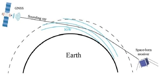
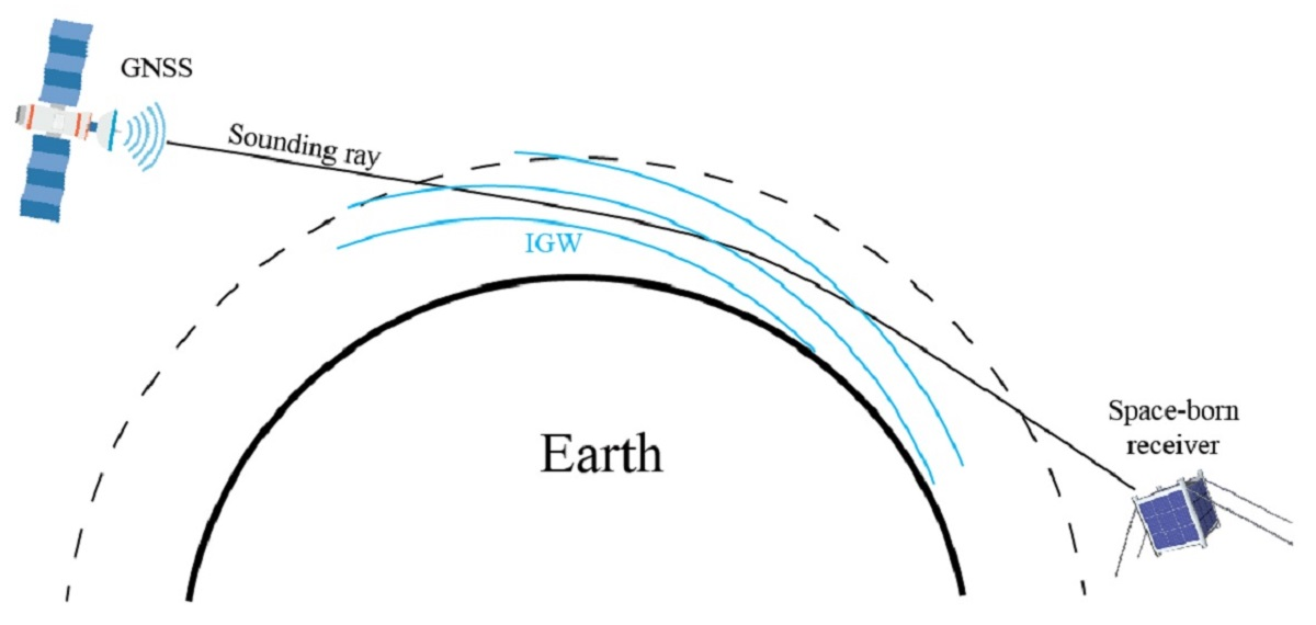
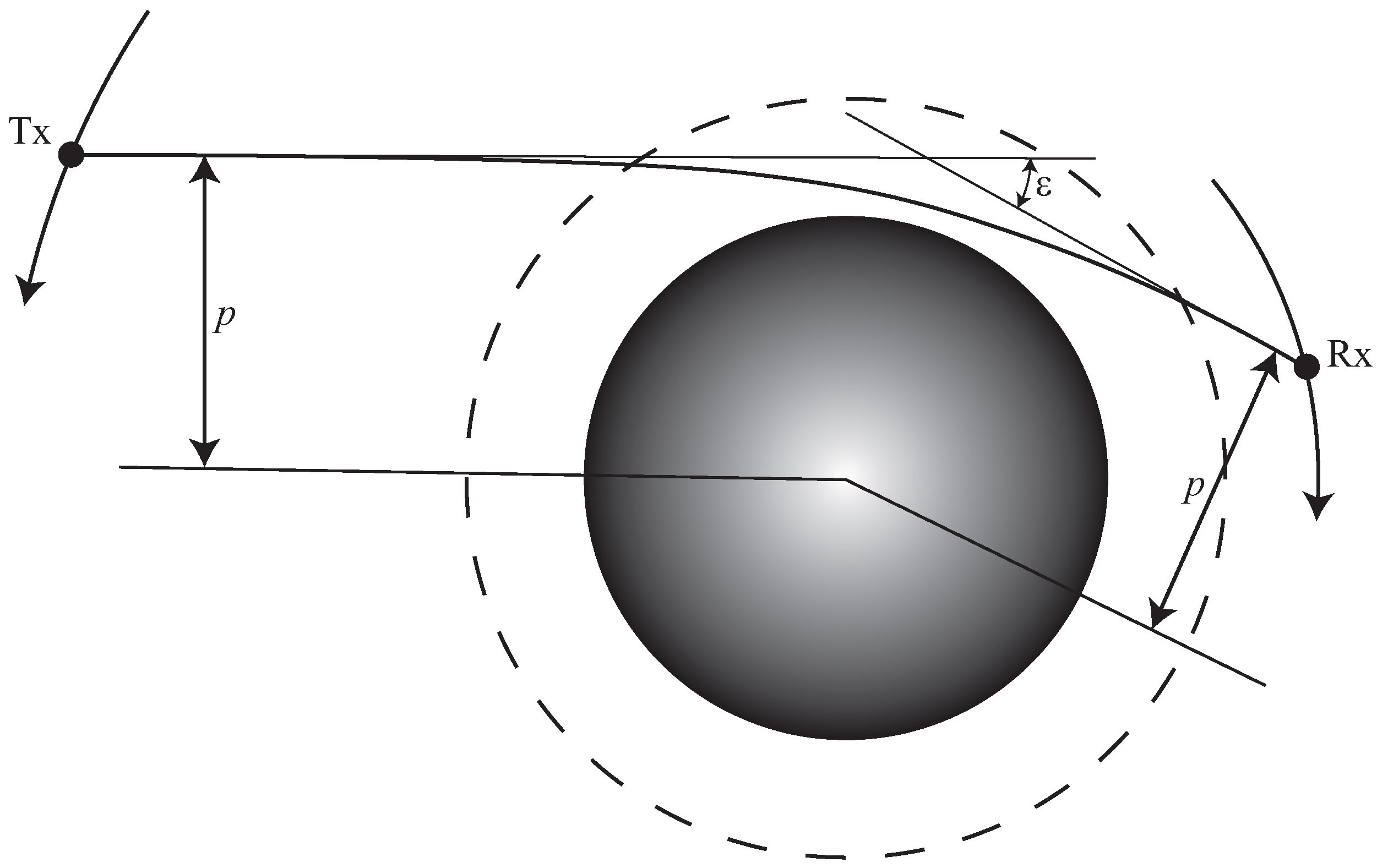
The RO principle is illustrated by Figure 1. The temperature retrieval is outlined as follows: First, the bending angle (BA) profile is evaluated, where p is the ray impact parameter (the ray leveling distance from the Earth’s center or the local curvature center [64]). To this end, a combination of geometric optical (GO) [65,66,67] and wave optical (WO) techniques [23,24,25,68,69] is applied. Usually, the GO technique is applied above 20 km, and the WO technique is applied below 20 km. In both cases, the BA is obtained from the derivative of the phase of the wave field, either originally measured or transformed by a Fourier Integral Operator [25]. The numerical differentiation of the noisy wave field involves its filtering. After obtaining BA for the two frequency channels, the ionospheric correction and statistical optimization algorithms are applied [65,70,71,72,73,74,75,76] in order to remove the ionospheric contribution and suppress the residual ionospheric noise, which becomes significant at altitudes above 30 km. The statistical optimization involves the estimates of the signal and error covariances, which can be static (fixed a priori profiles) or dynamic (estimated from actual observations). The resulting neutral atmospheric BA profile is the “optimal” linear combination of observations and the background BA estimate , which can be based on an existing climatological model of the Earth’s atmosphere [77,78] or on a large ensemble of RO observations [79,80]. Given the BA, the refractivity n is retrieved using the Abel integral [81,82,83]:
where is the refractive radius, and r is the distance from the local curvature center. Dependences and parametrically represent the profile . Instead of radius r, it is convenient to introduce the altitude , where is the local curvature radius. The retrieved refractivity n can be written as , where the unity corresponds to the vacuum and N is a function of the meteorological variables representing the medium:
Here, P is the full atmospheric pressure, is the partial pressure of water vapor, and K/hPa and K2/hPa are physical constants. Given , the temperature, under the assumption of a dry atmosphere, can be retrieved using the hydrostatic and state equations:
where is the density [84]. For the fluctuations of temperature we can write
This indicates that it is possible to study the spectra of relative fluctuations of refractivity.
Figure 1.
RO geometry. The transmitter Tx is one of the GNSS satellites. The receiver Rx is located on a low Earth orbiter. The radio ray between them is subject to refraction in the atmosphere. The bending angle and impact parameter p are derived from the measurements of the amplitude and phase of the received signal. Dependence measured during an occultation event is used in the retrieval.

This retrieval scheme relies upon the assumption of the spherical symmetry of the atmosphere. For a realistic atmosphere with horizontal gradients, we introduce the 2D field of refractivity in the occultation plane , where is the polar angle. The retrieved vertical profile is linked with by the following approximate relation [67]:
We conclude that the temperature retrieval from RO observations is based on the assumption of spherical symmetry and depends on the parameters controlling the filtering and the statistical optimization. The statistical optimization provides a trade-off between suppressing the residual ionospheric fluctuations and the retrieval of temperature profiles at large altitudes.
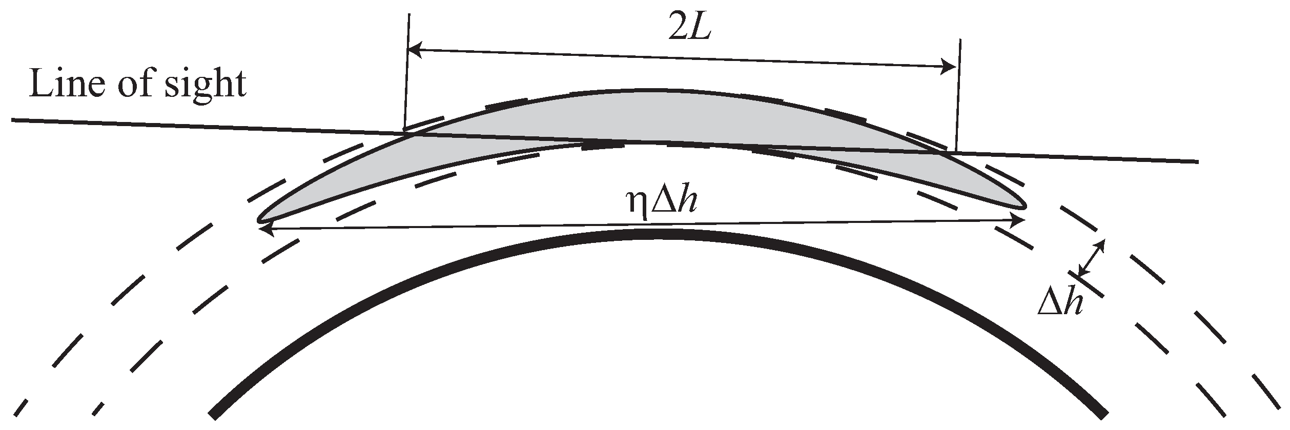
In order to estimate the IGW parameters that can be retrieved by 1D RO retrieval based on the assumption of spherical symmetry, we consider a structure with a vertical scale and anisotropy . The characteristic length of the interaction between a straight ray and a spherical layer with a thickness of is , where a is the Earth’s radius, as illustrated by Figure 2. For the retrieval of the anisotropic structure, it is required that . This results in the estimate of the anisotropy: . For the vertical scale km, the anisotropy must exceed a value of about , while for km, .
The first study of IGWs based on GPS/MET RO observations [85] was performed by Tsuda et al. [26], who utilized the retrieved profiles of temperature . The IGW activity was characterized by temperature variations with scales from 2 to 10 km. The values of and allowed the determination of and . An analysis of the seasonal, latitudinal, and height variations of was performed. The maximum height of the analysis was determined by the residual error of the ionospheric correction, which resulted in unrealistically large temperature variations above 45 km.
The Challenging Minisatellite Payload (CHAMP) [17] provided a larger amount of RO observations compared to the GPS/MET experiment, which promoted further studies of IGWs from RO observations. Another analysis based on temperature fluctuation was reported in [27], where the IGW activity was correlated with ionospheric perturbations. Ratnam et al. [28] presented a global analysis of GW activity in the stratosphere. Hei et al. [29] analyzed the atmospheric gravity wave activity in the polar regions in order to reveal the horizontal distribution and year-to-year variation of .
The Constellation Observing System for Meteorology Ionosphere and Climate (COSMIC) [86] made one more significant step in RO development by providing an enhanced data quality and amount. Khaykin et al. [30] analyzed the temperature fluctuations based on the COSMIC observations for the years 2006–2013, complemented with data from the Rayleigh lidar at the Haute-Provence observatory. Seasonal variations of were studied.
Alexander et al. [31] analyzed 6 years (2007–2012) of COSMIC observations in the region to the east of the Andes range in the Southern Hemisphere, indicating favorable conditions for IGW generation, in order to verify the IGW activity surplus in the east with respect to the west. The RO events were classified as belonging to the east or west sector. A question was posed about the uncertainty of the decomposition of retrieved temperature profiles into the background and waves, in view of the intermittent nature of IGWs and the presence of ubiquitous mesoscale structures not related to IGWs. Another issue is linked to the probability distribution of , which has a skew shape and may be better characterized by its median rather than its mean. The drop in the distribution for a small energy may reflect the limited accuracy of the RO temperature retrievals rather than the true physics. The observation data were classified in terms of season, favorable or unfavorable line of sight, and location to the west or east of the Andes range. Three different schemes for the interpretation of RO data as IGW indicators were analyzed: non-parametric, log-normal distribution, and exponential distribution. It was concluded that the right choice of the distribution derived from RO at the lowest values may improve the possible detection of GW activity.
Rapp et al. [32] analyzed the data of Meteorological Operational Satellites (METOP) A and B operated by the European Organisation for the Exploitation of Meteorological Satellites (EUMETSAT) [18]. The values of retrieved from RO temperatures were compared with the operational analysis of the Integrated Forecast System (IFS) and reanalysis (ERA-Interim) of the European Centre for Medium-Range Weather Forecasts (ECMWF). The agreement of the RO temperatures with the ERA-Interim and IFS temperatures was established. It was also noticed that ERA-Interim data suffer from a much coarser resolution as compared to IFS data. A comparison of the derived from RO with the ground-based Rayleigh lidar observations indicated that the patterns of the seasonal variations were very similar, but the lidar gave approximately two-times higher values of . This can be explained by the fact the lidar retrieves local temperature variations, which must be larger compared to those retrieved from RO limb observations, producing values averaged over a horizontal distance of about 300 km. Good agreement between the derived from RO and that from the IFS was found at the altitude of 22 km, while at the altitudes of 28 and 38 km, where RO data are subject to the residual errors of the ionospheric correction, the agreement was noticeably worse.
Yu et al. [33] analyzed COSMIC data for the years 2007–2013 and found a statistically significant correlation between the and tropopause parameters, including lapse rate or cold-point tropopause height and temperature. Luo et al. [34] performed an analysis of the spatio-temporal distribution of the global at altitudes of 20–35 km, using temperature profiles from CHAMP, COSMIC, and METOP-A/B/C during the period 2007–2020. The linear trends of and its responses to the solar activity, quasi biennial oscillation (QBO), and El Niño–Southern Oscillation (ENSO) were found. Chen et al. [35] studied IGW activity in the Tibetan Plateau using derived from the temperature profiles obtained by COSMIC and METOP-A/B/C missions from August 2006 to September 2020.
Rapp et al. [36] drew attention to the inertial instability (II), which may result in temperature perturbation at scales below 10–15 km not related to IGWs. II is generated by an imbalance of pressure gradient and Coriolis forces in an axisymmetric vortex or anticyclonically sheared zonal geostrophic flow [37]. The study was based on METOP-A/B data and ECMWF operational analyses for December 2015. RO observations may indicate large stratospheric temperature perturbations with vertical scales below 15 km and an amplitude of about 10 K. Using high-resolution ECMWF operational analyses, it was demonstrated that these events are generated from II caused by the large meridional shear of the zonal wind at the southern edge of an exceptionally strong polar night jet in combination with Rossby wave breaking. It was concluded that II is an important source of stratospheric temperature variability at km from mid-October to mid-April at midlatitudes at 30–45°N and from mid-April to mid-October at 30–45°S.
3.2. Retrieved Temperature Fluctuation Spectra
Steiner and Kirchengast [38] presented a study of GPS/MET temperature fluctuation spectra, which were expected to obey the power law for saturated IGWs (5):
The evaluation of the fluctuation spectra was only possible in a limited wavenumber interval from 0.1 to 1.0 cycle/km, which corresponds to vertical scales from 1 to 10 km. The GO retrieval limited the vertical resolution by a scale of about 1.5 km. The resulting spectra deviated from the expected power law : (1) they had a plateau for a low frequency corresponding to wavelengths exceeding 5 km, and (2) they had a steeper decrease after the plateau. This illustrates the degree of the influence of the “observation filter” [1] upon the temperature retrieval. As argued by Šácha et al. [41], it can also be attributed to the use of the hydrostatic balance assumption.
Another study of GPS/MET temperature fluctuation spectra was presented by Tsuda and Hocke [39]. They used a shorter smoothing window in the temperature profile retrieval, as compared to that adopted by the University Corporation of Atmospheric Research (UCAR). This resulted in a much better agreement with the theoretical power spectrum of . However, Marquardt and Healy [87] argued that the reported spectra with sub-Fresnel vertical wavelengths as low as 400 m are beyond the capability of the GO technique, and the spectral slope of is rather the signature of the measurement noise. Tsuda et al. [40] applied WO processing to COSMIC observations in the altitude range of 20–30 km and obtained spectra that were much closer to the theoretical values, reaching a frequency of cycle/m, which corresponds to a scale of 250 m. A comparison with GO spectra indicated that the WO technique also provided better agreement with the theory for scales exceeding the Fresnel scale. Still, the residual errors of the ionospheric correction should affect scales below 1 km [88]. Another question regards the propagation of the measurement noise through the WO retrieval chain [89].
The question regarding the influence of the hydrostatic balance assumption upon IGW retrieval was first posed by Šácha et al. [41] and studied further by Pisoft et al. [42]. To this end, radiosonde data were employed, and the spectra of the real profiles and those derived from the hydrostatic equation were evaluated. The differences were found to be insignificant, especially when averaging over a large ensemble of profiles.
3.3. Space–Frequency Analysis
Wang and Alexander [43] analyzed COSMIC and CHAMP temperatures, employing S-transform analysis [90] to derive the complete set of IGW parameters, including horizontal propagation direction. The study was motivated by the fact that filtering temperature profiles with respect to alone does not separate global-scale waves (like Kelvin waves) and IGWs.
The S-transform is a wavelet-like short-term Fourier transform with the Gaussian weight function. Given a function , its S-transform as a function of time t and frequency is expressed as follows:
Its integral over t equals the Fourier transform , which allows the recovery of from :
It possesses, therefore, only one of the two required properties of the “classical” time–frequency distributions [91]. The S-transform is sensitive to the absolute phase of the signal , which plays a crucial role in further considerations. The cross-S-transform for two signals and is defined as , where the asterisk stays for the complex conjugate.
The combined COSMIC and CHAMP data provided a significant amount of profiles, which allowed the definition of the background temperatures on the basis of horizontal scale, suppressing the global-scale waves. The temperature profiles were interpolated to a regular vertical grid with a 200 m resolution and collected within latitude–longitude bins . These data for each latitude and longitude were then subjected to the S-transform along the longitude, recovering zonal harmonics as functions of the latitude and longitude. Subsequently, zonal wave numbers from 0 to 6 were treated as the background field including the global-scale waves. The IGW temperature and the wavelength of the dominant mode were also determined by means of the S-transform. The analysis comprised vertical scales from 4 to 15 km.
The application of the cross-S-transform in [43] allowed the estimation of the horizontal wavelengths of the IGWs. It was based on the phase differences between the i-th and j-th event for the dominant vertical wave number in the selected group of events representing the same IGW. The horizontal wave vector was inferred from the overdetermined linear system:
For the altitude range of 17.5–22.5 km, the vertical wavelength was found to vary from 4.8 km to 8.4 km, while varied from 1500 to 4500 km. This indicates that the revealed IGWs were highly anisotropic structures with approaching , which are easily retrieved from RO observations.
The technique of the S-transform was further employed in [44] in order to identify collocated pairs of COSMIC RO events observing the same IGW. Event pairs with a time difference below 15 min and spatial separation below 250 km were selected. The identification of coherent IGWs was based on the cross-S-transform technique. The noise level was determined by the first-order autoregressive model involving a Monte Carlo simulation based on the IGW spectrum. This allowed the determination of the dominant wavelength . The phase shift between the profiles together with their spatial separation determined the horizontal wavelength, similarly to (22). This demonstrated the importance of coherency analysis for the identification of event pairs affected by the same IGW. The calculated distribution of the horizontal wavelengths comprised scales from 1000 km to about 4000 km with a median value of approximately 1200 km and a mean of 1580 km. This approach may help to avoid the assumption that a dominant monochromatic wave exists in each longitude–latitude–time cell at a given height [43].
The technique of the determination of horizontal and vertical wavelengths was applied in [49] to estimate the Momentum Flux (MF). The MF is expressed as follows:
The expression for the IGW temperature amplitude is [62]
Together with (10), this results in the following relationship:
Therefore, IGWs with a smaller anisotropy and a larger vertical wavelength provide a maximum contribution to the MF.
The continuous wavelet transform (CWT) for the identification of individual waves and the evaluation of their MF was applied in [46]. An eighth-order complex Gaussian wavelet, which retains the phase information, was chosen. The CWT was applied to the detrended and normalized temperature perturbation profile, windowed with a Gaussian of full width at half maximum of 22 km, centered at a height of 30 km. This method was thus sensitive to IGWs at heights of around 30 km. The magnitudes of spectral coefficients were evaluated and treated as pseudo-correlation coefficients ranging between 0 and 1. Values exceeding 0.6 identified individual waves. The method was applied to COSMIC observations for June–August 2006–2012, and at 30 km was evaluated. In order to evaluate the MF, cross-wavelet analysis was applied: for two profiles and , the cross-wavelet coefficients (cospectra) were defined as follows:
where and are the complex wavelet spectra for two events, and is the phase difference. This allowed the evaluation of the horizontal wave number and MF, similarly to [49].
The CWT technique was employed in [47] for the identification of IGWs in a case study. Further studies that employed the horizontal wave number evaluation from the phase differences between different profiles for the derivation of the MF are [45,48].
Nath et al. [50] analyzed CHAMP (September 2001–August 2006) and COSMIC (September 2006–March 2010) data, involving ground-based soundings of the zonal and meridional wind and temperature, NOAA satellite observations of interpolated outgoing long-wave radiation, and ECMWF reanalysis datasets (ERA-interim). The study used the techniques described in [92,93]. The analysis was based on the temperature fluctuations obtained by subtracting the zonal mean temperature profiles at each height and for each day. The aims of the study included: (a) space–time symmetric and antisymmetric spectra about the equator over a latitude band of 10°S–10°N, to extract equatorial wave modes (the Kelvin waves (KWs), mixed Rossby–gravity waves (MRGWs), equatorial Rossby waves (ERWs), and IGWs); (b) wave–mean flow interaction and momentum flux estimation; (c) latitudinal and seasonal variability; and (d) the longitudinal and seasonal distribution of atmospheric gravity wave energy density in the tropical lower stratosphere, and its long-term variation in relation to convective activity, during the different phases of QBO. The spectra were represented as a superposition of the symmetric and antisymmetric components responsible for different type of waves. The odd meridional mode numbers in the symmetric spectra described KWs (−1), ERWs (1), and IGWs (1). The even meridional mode 0 in the symmetric spectra described the MRGWs. The vertical wave number was derived by using the dispersion relation (4). This allowed the study of the long-term variations of the IGW potential energy and MF.
3.4. Wave Parameter Estimates
Gubenko et al. [51,52] developed a technique for the determination of the intrinsic frequency and other wave parameters for a single event, under the assumption that there is a single dominant wave. To this end, they utilized the relation for the horizontal velocity perturbation amplitude under the assumption that [94]:
The shear instability threshold of the ratio a of the horizontal velocity perturbation and the IGW intrinsic velocity assuming a minimum Richardson number of was derived in [95]:
On the other hand, the following expression can be written:
where , and all the values in the right-hand part can be determined from an RO temperature profile. The observed temperature fluctuations in the low stratosphere may be related to IGWs only if the following relation holds:
In this case, it is possible to determine the intrinsic frequency, the intrinsic horizontal phase speed, the vertical phase speed, and the amplitude of the horizontal velocity perturbation:
This technique can be combined with the space–frequency analysis discussed above.
3.5. Studies Based on Diffraction Theory
Kan et al. [53,54,55] derived IGW parameters from RO observation using the approach based on the diffraction theory, initially developed by Gurvich and Kan [11,12], Sofieva et al. [13], Gurvich and Brekhovskikh [58] for the interpretation of stellar occultations. The studies adopted the constant anisotropy spectrum (6) of the relative fluctuations of refractivity or temperature. The Fresnel scale for RO observation geometry and the wavelengths of GNSSs is about 1.5 km and significantly exceeds the IGW internal scale of 10–100 m in the stratosphere, which need not be taken into account, as pointed out following (6).
By integrating over horizontal wavenumbers , we arrive at the 1D single-sided vertical spectrum, which generalizes (18):
The external scale in the stratosphere is a few kilometers [2]. This parameter defines the transition between the unsaturated and saturated modes. Finally, the structural characteristic remains the only parameter characterizing the 1D spectrum in the saturation mode. Using (18), we arrive at the following expression:
The analysis of star scintillations [96,97] resulted in the conclusion that the anisotropy coefficient increases with the vertical scale and saturates for scales of about 100 m, while its maximum value (8) is typically several hundred in the stratosphere. This indicates that the anisotropy exceeds its critical value [58], and the observed signal fluctuations become independent from the anisotropy.
The basic approximations are the phase screen and weak fluctuations [58]. The 3D atmosphere is approximately represented as a thin screen with the equivalent eikonal thickness, located near the ray perigee. The fluctuation spectrum of the eikonal can be written as follows:
where is the mean eikonal.
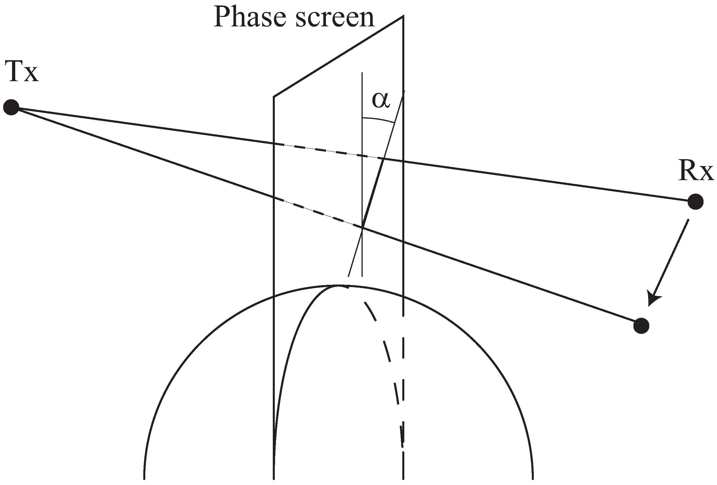
In an RO experiment, the amplitude A of the radio signal is measured. The fluctuations of the logarithm of the relative amplitude are considered weak if . The projection of the ray perigees during an occultation event to the phase screen is a line at an angle with respect to the local vertical, as shown in Figure 3. If , the occultation event can be considered vertical (i.e., the amplitude can be considered a function of the ray perigee altitude only). This condition is satisfied for , eventually, for all valid RO events. Then, the amplitude fluctuation spectrum can be written as follows:
where is the wavenumber, is the wavelength, , is the vertical Fresnel scale, q is the refractive attenuation, is the reduced observation distance, and are the distances from the receiver R and transmitter T to the ray perigee. Finally, the expression for the relative amplitude fluctuation spectra takes the following form:
The two parameters of the IGW spectrum (35), and , allow the derivation of the specific potential energy , using (10) and (36):
Figure 3.
The phase screen geometry. The projections of the ray perigees to the phase screen during an occultation event form a line at an angle with respect to the local vertical.
Figure 3.
The phase screen geometry. The projections of the ray perigees to the phase screen during an occultation event form a line at an angle with respect to the local vertical.

These two parameters can be determined from experimental estimates of amplitude fluctuation spectra (39). This is simpler than for star occultations, because there is no need for taking into account the Kolomogorov turbulence, whose influence upon RO observation is negligible due to a relatively long sounding radio wave, as compared to the optic range. On the other hand, the ionospheric scintillations and the proximity of the Fresnel scale and the external scale constitute error sources. In order to determine and , the theoretical spectra are fitted to the observational spectra averaged in spatial–seasonal cells.
Kan et al. [53] analyzed COSMIC data for 15 days equally apportioned over spring 2011, with a total of about 27,000 events. The data were subdivided into latitude zones –, –, –, and –. The observational data were used below the height of 32 km, where the ionospheric influence is small. The lower height was chosen to be 1 km above the tropopause, in order to remove large temperature gradients. The spectra were evaluated for fragments of observational records with a length of 8 km and with a 2 km step. Finally, the minimum height for the spectral parameter estimates varied from 16 km in the polar zones to 22 km in the tropics, and the maximum height was 28 km. This allowed the estimation of , which varied from about 2 km in the polar zones to about 3.5 km in the tropics. Kan et al. [54] performed a more detailed statistical analysis of COSMIC data, including the profiles of , , and temperature variance for different latitudinal zones for all the seasons.
4. Discussion and Conclusions
RO observations provide an unique opportunity for the global monitoring of IGWs. The COSMIC Data Analysis and Archive Center (CDAAC) provides open access to the observations from a series of RO missions. These include both accomplished (GPS/MET, CHAMP, COSMIC, METOP-A) and active (COSMIC-2, METOP-B/C, Spire, GeoOptics [98], PlanetIQ [99]) missions. This provides time series long enough for climatological studies of IGWs.
In this review, we concentrated on different techniques for the retrieval of the IGW characteristics from RO observations. A general limitation of the RO technique is linked to the ionospheric perturbations. Although standard RO processing algorithms include the ionospheric correction, the residual error becomes significant at altitudes above ∼35 km. The simplest approach to IGW retrieval uses temperature perturbations with respect to a background, describing large-scale temperature perturbations that cannot be attributed to IGWs. A series of studies derived the IGW specific potential energy and its climatologies from temperature perturbations. This approach is a good illustration of the concept of the observation filter. The temperature profiles were obtained from RO observations as a result of a complicated retrieval algorithm including numerical differentiation with a specific smoothing window. In addition, in the GO retrieval scheme, the Fresnel scale imposed a resolution limitation. The application of the GO technique resulted in temperature fluctuation spectra with a variable slope, instead of the expected power law . The Fresnel resolution limitation was lifted by the WO technique, and its application improved the agreement of the spectra with the theory. However, scales below 1 km are affected by the residual errors of the ionospheric correction. Moreover, the IGW spectrum has a steep slope, and its integral parameters, like , are determined by large scales.
The main question regarding this approach is how to distinguish IGWs from other processes. In particular, II can result in large non-IGW temperature perturbations. A question was also posed as to whether the hydrostatic balance assumption is valid for IGWs.
A more advanced approach aiming to answer this question was based on the space–frequency analysis of 4D spatio-temporal fields of temperature retrieved from a large number of RO events. The analysis employed the S-transform or CWT and allowed the identification of propagating IGWs exploiting the phase differences and dispersion relations. These studies demonstrated that IGWs are highly anisotropic structures, favorable for RO retrievals. This approach, complemented by the analysis of spectral symmetries, resulted in distinguishing between IGWs and planetary waves, like KWs, MRGWs, and ERWs. The technique of the simultaneous determination of the horizontal and vertical wavelengths allowed the derivation of the MF.
Several studies exploited additional physical restrictions linked to the stability condition expressed in terms of the Richardson number. This allowed the formulation of a necessary condition that the IGW must obey, as well as the derivation of such parameters as the intrinsic frequency, the intrinsic horizontal phase speed, the vertical phase speed, and the amplitude of the horizontal velocity perturbation.
Another direction of IGW parameter retrieval was based on the application of the diffraction theory. This technique was initially developed for stellar occultations. The simple approximations of the phase screen and weak fluctuations result in a closed analytical expression for the amplitude fluctuation spectra, in terms of two parameters of the IGW spectra: external scale and structural characteristic . These parameters are obtained by fitting the observed spectra averaged over some spatial and seasonal cells. The obtained amplitude fluctuation spectra agree with the assumption of an IGW with large anisotropy. This technique has an advantage over the temperature-based approach: it operates on the raw observations of the amplitude without any processing. Its disadvantage is that the Fresnel scale for the RO observation geometry is close to . However, this can be overcome by applying the Back Propagation (BP) method [100].
We conclude that the derivation of IGWs from RO observation is widely performed and has been stimulated by the large number of RO observations. It applies advanced techniques based on Fourier and space–time analysis, physical equations describing IGWs, and the diffraction theory, which have contributed to the success of IGW study based on RO.
Author Contributions
Conceptualization, V.K.; methodology, V.K. and M.G.; formal analysis, M.G.; writing—original draft preparation, M.G.; writing—review and editing, M.G. and V.K. All authors have read and agreed to the published version of the manuscript.
Funding
This research received no external funding.
Data Availability Statement
This review did not use any external data sets.
Acknowledgments
The author is grateful to Stephen Leroy (AER) for useful discussions on IGW retrieval techniques from RO observations.
Conflicts of Interest
The authors declare no conflicts of interest.
Abbreviations
The following abbreviations are used in this manuscript:
| BA | Bending angle |
| CDAAC | COSMIC Data Analysis and Archive Center |
| CHAMP | Challenging Minisatellite Payload |
| COSMIC | Constellation Observing System for Meteorology Ionosphere and Climate |
| CWT | Continuous wavelet transform |
| ECMWF | European Centre for Medium-Range Weather Forecasts |
| ENSO | El Niño–Southern Oscillation |
| ERA | ECMWF reanalysis |
| ERW | Equatorial Rossby waves |
| EUMETSAT | European Organisation for the Exploitation of Meteorological Satellites |
| GNSS | Global Navigation Satellite System |
| GO | Geometric optics |
| GPS/MET | GPS Meteorology |
| IFS | Integrated Forecast System |
| IGW | Internal gravity wave |
| II | Inertial instability |
| KW | Kelvin wave |
| METOP | Meteorological operational satellite |
| MF | Momentum flux |
| MRGW | Mixed Rossby–gravity wave |
| QBO | Quasi-biennial oscillation |
| RO | Radio occultation |
| UCAR | University Corporation of Atmospheric Research |
| WO | Wave optics |
References
- Fritts, D.C.; Alexander, M.J. Gravity waves dynamics and effects in the middle atmosphere. Rev. Geophys. 2003, 41, 1003. [Google Scholar] [CrossRef]
- Tsuda, T.; VanZandt, T.E.; Mizumoto, M.; Kato, S.; Fukao, S. Spectral analysis of temperature and Brunt-Vaisala frequency fluctuations observed by radiosondes. J. Geophys. Res. Atmos. 1991, 96, 17265–17278. [Google Scholar] [CrossRef]
- Vincent, R.A.; Alexander, M.J. Gravity waves in the tropical lower stratosphere: An observational study of seasonal and interannual variability. J. Geophys. Res. Atmos. 2000, 105, 17971–17982. [Google Scholar] [CrossRef]
- Wang, L.; Geller, M.A.; Alexander, M.J. Spatial and Temporal Variations of Gravity Wave Parameters. Part I: Intrinsic Frequency, Wavelength, and Vertical Propagation Direction. J. Atmos. Sci. 2005, 62, 125–142. [Google Scholar] [CrossRef]
- Fritts, D.C.; Tsuda, T.; Zandt, T.E.V.; Smith, S.A.; Sato, T.; Fukao, S.; Sato, K. Studies of velocity fluctuations in the lower atmosphere using the MU radar. II. Momentum fluxes and energy densities. J. Atmos. Sci. 1990, 47, 51–66. [Google Scholar] [CrossRef]
- Murayama, Y.; Tsuda, T.; Fukao, S. Seasonal variation of gravity wave activity in the lower atmosphere observed with the MU radar. J. Geophys. Res. Atmos. 1994, 99, 23057–23069. [Google Scholar] [CrossRef]
- Bacmeister, J.T.; Eckermann, S.D.; Newman, P.A.; Lait, L.; Chan, K.R.; Loewenstein, M.; Proffitt, M.H.; Gary, B.L. Stratospheric horizontal wavenumber spectra of winds, potential temperature and atmospheric tracers observed by high-altitude aircraft. J. Geophys. Res. 1996, 101, 9441–9470. [Google Scholar] [CrossRef]
- Cho, J.Y.N.; Zhu, Y.; Newell, R.E.; Anderson, B.E.; Barrick, J.D.; Gregory, G.L.; Sachse, G.W.; Carroll, M.A.; Albercook, G.M. Horizontal wavenumber spectra of winds, temperature, and trace gases during the Pacific Exploratory Missions: 1. Climatology. J. Geophys. Res. Atmos. 1999, 104, 5697–5716. [Google Scholar] [CrossRef]
- Alexander, M.J.; Gille, J.; Cavanaugh, C.; Coffey, M.; Craig, C.; Eden, T.; Francis, G.; Halvorson, C.; Hannigan, J.; Khosravi, R.; et al. Global estimates of gravity wave momentum flux from High Resolution Dynamics Limb Sounder observations. J. Geophys. Res. 2008, 113, D15S18. [Google Scholar] [CrossRef]
- Ern, M.; Preusse, P.; Alexander, M.J.; Warner, C.D. Absolute values of gravity wave momentum flux derived from satellite data. J. Geophys. Res. 2004, 109, D20103. [Google Scholar] [CrossRef]
- Gurvich, A.S.; Kan, V. Structure of air density irregularities in the stratosphere from spacecraft observations of stellar scintillation: 1. Three-dimensional spectrum model and recovery of its parameters. Izv. Atm. Ocean. Phys. 2003, 39, 300–310. [Google Scholar]
- Gurvich, A.S.; Kan, V. Structure of air density irregularities in the stratosphere from spacecraft observations of stellar scintillation: 2. Characteristic scales, structure characteristics, and kinetic energy dissipation. Izv. Atm. Ocean. Phys. 2003, 39, 311–321. [Google Scholar]
- Sofieva, V.F.; Gurvich, A.S.; Dalaudier, F.; Kan, V. Reconstruction of internal gravity wave and turbulence parameters in the stratosphere using GOMOS scintillation measurements. J. Geophys. Res. 2007, 112, D12113. [Google Scholar] [CrossRef]
- Sofieva, V.F.; Kyrölä, E.; Hassinen, S.; Backman, L.; Tamminen, J.; Seppälä, A.; Thölix, L.; Gurvich, A.S.; Kan, V.; Dalaudier, F.; et al. Global analysis of scintillation variance: Indication of gravity wave breaking in the polar winter upper stratosphere. Geophys. Res. Lett. 2007, 34, L03812. [Google Scholar] [CrossRef]
- Rocken, C.; Anthes, R.; Exner, M.; Hunt, D.; Sokolovskiy, S.; Ware, R.; Gorbunov, M.; Schreiner, W.; Feng, D.; Herman, B.; et al. Analysis and validation of GPS/MET data in the neutral atmosphere. J. Geophys. Res. Atmos. 1997, 102, 29849–29866. [Google Scholar] [CrossRef]
- Yunck, T.; Liu, C.; Ware, R. A History of GPS Sounding. Terr. Atmos. Ocean. Sci. 2000, 11, 1–20. [Google Scholar] [CrossRef]
- Wickert, J.; Reigber, C.; Beyerle, G.; Konig, R.; Marquardt, C.; Schmidt, T.; Grunwaldt, L.; Galas, R.; Meehan, T.K.; Melbourne, W.G.; et al. Atmosphere sounding by GPS radio occultation: First results from CHAMP. Geophys. Res. Lett. 2001, 28, 3263–3266. [Google Scholar] [CrossRef]
- Bonnedal, M.; Christensen, J.; Carlström, A.; Berg, A. Metop-GRAS in-orbit instrument performance. GPS Solut. 2010, 14, 109–120. [Google Scholar] [CrossRef]
- Chu, C.H.; Fong, C.J.; Xia-Serafino, W.; Shiau, A.; Taylor, M.; Chang, M.S.; Chen, W.J.; Liu, T.Y.; Liu, N.C.; Martins, B.; et al. An Era of Constellation Observation-FORMOSAT-3/COSMIC and FORMOSAT-7/COSMIC-2. J. Aeronaut. Astrnaut. Aviat. 2018. [Google Scholar] [CrossRef]
- Fong, C.J.; Chu, C.H.; Lin, C.L.; da Silva Curiel, A. Toward the Most Accurate Thermometer in Space: FORMOSAT-7/COSMIC-2 Constellation. IEEE Aerosp. Electron. Syst. Mag. 2019, 34, 12–20. [Google Scholar] [CrossRef]
- Ho, S.P.; Zhou, X.; Shao, X.; Zhang, B.; Adhikari, L.; Kireev, S.; He, Y.; Yoe, J.G.; Xia-Serafino, W.; Lynch, E. Initial Assessment of the COSMIC-2/FORMOSAT-7 Neutral Atmosphere Data Quality in NESDIS/STAR Using In Situ and Satellite Data. Remote Sens. 2020, 12, 4099. [Google Scholar] [CrossRef]
- Qiu, C.; Wang, X.; Zhou, K.; Zhang, J.; Chen, Y.; Li, H.; Liu, D.; Yuan, H. Comparative Assessment of Spire and COSMIC-2 Radio Occultation Data Quality. Remote Sens. 2023, 15, 5082. [Google Scholar] [CrossRef]
- Gorbunov, M.E. Canonical transform method for processing radio occultation data in the lower troposphere. Radio Sci. 2002, 37, 1–10. [Google Scholar] [CrossRef]
- Jensen, A.S.; Lohmann, M.S.; Nielsen, A.S.; Benzon, H.H. Geometrical optics phase matching of radio occultation signals. Radio Sci. 2004, 39, RS3009. [Google Scholar] [CrossRef]
- Gorbunov, M.E.; Lauritsen, K.B. Analysis of wave fields by Fourier integral operators and its application for radio occultations. Radio Sci. 2004, 39, RS4010. [Google Scholar] [CrossRef]
- Tsuda, T.; Nishida, M.; Rocken, C.; Ware, R.H. A global morphology of gravity wave activity in the stratosphere revealed by the GPS occultation data (GPS/MET). J. Geophys. Res. Atmos. 2000, 105, 7257–7273. [Google Scholar] [CrossRef]
- Hocke, K.; Tsuda, T. Gravity waves and ionospheric irregularities over tropical convection zones observed by GPS/MET radio occultation. Geophys. Res. Lett. 2001, 28, 2815–2818. [Google Scholar] [CrossRef]
- Ratnam, M.V.; Tetzlaff, G.; Jacobi, C. Global and Seasonal Variations of Stratospheric Gravity Wave Activity Deduced from the CHAMP/GPS Satellite. J. Atmospheric Sci. 2004, 61, 1610–1620. [Google Scholar] [CrossRef]
- Hei, H.; Tsuda, T.; Hirooka, T. Characteristics of atmospheric gravity wave activity in the polar regions revealed by GPS radio occultation data with CHAMP. J. Geophys. Res. 2008, 113, D04107. [Google Scholar] [CrossRef]
- Khaykin, S.M.; Hauchecorne, A.; Mzé, N.; Keckhut, P. Seasonal variation of gravity wave activity at midlatitudes from 7years of COSMIC GPS and Rayleigh lidar temperature observations. Geophys. Res. Lett. 2015, 42, 1251–1258. [Google Scholar] [CrossRef]
- Alexander, P.; de la Torre, A.; Hierro, R.; Llamedo, P. An improvement of the sensitivity of GPS radio occultation data to detect gravity waves through observational and modeling factors. Adv. Space Res. 2016, 57, 543–551. [Google Scholar] [CrossRef]
- Rapp, M.; Dörnbrack, A.; Kaifler, B. An intercomparison of stratospheric gravity wave potential energy densities from METOP GPS radio occultation measurements and ECMWF model data. Atmos. Meas. Tech. 2018, 11, 1031–1048. [Google Scholar] [CrossRef]
- Yu, D.; Xu, X.; Luo, J.; Li, J. On the Relationship between Gravity Waves and Tropopause Height and Temperature over the Globe Revealed by COSMIC Radio Occultation Measurements. Atmosphere 2019, 10, 75. [Google Scholar] [CrossRef]
- Luo, J.; Hou, J.; Xu, X. Variations in Stratospheric Gravity Waves Derived from Temperature Observations of Multi-GNSS Radio Occultation Missions. Remote Sens. 2021, 13, 4835. [Google Scholar] [CrossRef]
- Chen, Z.; Gao, Y.; Li, L.; He, X.; Yang, W.; Luo, H.; Gong, X.; Lv, K. An Investigation of the Lower Stratospheric Gravity Wave Activity in Tibetan Plateau Based on Multi-GNSS RO Dry Temperature Observations. Remote Sens. 2022, 14, 5671. [Google Scholar] [CrossRef]
- Rapp, M.; Dörnbrack, A.; Preusse, P. Large Midlatitude Stratospheric Temperature Variability Caused by Inertial Instability: A Potential Source of Bias for Gravity Wave Climatologies. Geophys. Res. Lett. 2018, 45, 682–690. [Google Scholar] [CrossRef]
- Harvey, V.L.; Knox, J.A. Beware of Inertial Instability Masquerading as Gravity Waves in Stratospheric Temperature Perturbations. Geophys. Res. Lett. 2019, 46, 1740–1745. [Google Scholar] [CrossRef]
- Steiner, A.K.; Kirchengast, G. Gravity Wave Spectra from GPS/MET Occultation Observations. J. Atmos. Oceanic Technol. 2000, 17, 495–503. [Google Scholar] [CrossRef]
- Tsuda, T.; Hocke, K. Vertical Wave Number Spectrum of Temperature Fluctuations in the Stratosphere using GPS Occultation Data. J. Meteor. Soc. Japan. Ser. II 2002, 80, 925–938. [Google Scholar] [CrossRef]
- Tsuda, T.; Lin, X.; Hayashi, H. Analysis of vertical wave number spectrum of atmospheric gravity waves in the stratosphere using COSMIC GPS radio occultation data. Atmos. Meas. Tech. 2011, 4, 1627–1636. [Google Scholar] [CrossRef]
- Šácha, P.; Foelsche, U.; Pišoft, P. Analysis of internal gravity waves with GPS RO density profiles. Atmos. Meas. Tech. 2014, 7, 4123–4132. [Google Scholar] [CrossRef]
- Pisoft, P.; Sacha, P.; Miksovsky, J.; Huszar, P.; Scherllin-Pirscher, B.; Foelsche, U. Revisiting internal gravity waves analysis using GPS RO density profiles: Comparison with temperature profiles and application for wave field stability study. Atmos. Meas. Tech. 2018, 11, 515–527. [Google Scholar] [CrossRef]
- Wang, L.; Alexander, M.J. Global estimates of gravity wave parameters from GPS radio occultation temperature data. J. Geophys. Res. 2010, 115, D21122. [Google Scholar] [CrossRef]
- McDonald, A.J. Gravity wave occurrence statistics derived from paired COSMIC/FORMOSAT3 observations. J. Geophys. Res. 2012, 117, D15406. [Google Scholar] [CrossRef]
- Faber, A.; Llamedo, P.; Schmidt, T.; de la Torre, A.; Wickert, J. On the determination of gravity wave momentum flux from GPS radio occultation data. Atmos. Meas. Tech. 2013, 6, 3169–3180. [Google Scholar] [CrossRef]
- Hindley, N.P.; Wright, C.J.; Smith, N.D.; Mitchell, N.J. The southern stratospheric gravity wave hot spot: Individual waves and their momentum fluxes measured by COSMIC GPS-RO. Atmos. Chem. Phys. 2015, 15, 7797–7818. [Google Scholar] [CrossRef]
- Hierro, R.; Steiner, A.K.; de la Torre, A.; Alexander, P.; Llamedo, P.; Cremades, P. Orographic and convective gravity waves above the Alps and Andes Mountains during GPS radio occultation events – a case study. Atmos. Meas. Tech. 2018, 11, 3523–3539. [Google Scholar] [CrossRef]
- Alexander, P.; Schmidt, T.; de la Torre, A. A Method to Determine Gravity Wave Net Momentum Flux, Propagation Direction, and “Real” Wavelengths: A GPS Radio Occultations Soundings Case Study. Earth Space Sci. 2018, 5, 222–230. [Google Scholar] [CrossRef]
- Schmidt, T.; Alexander, P.; Torre, A. Stratospheric gravity wave momentum flux from radio occultations. J. Geophys. Res. Atmos. 2016, 121, 4443–4467. [Google Scholar] [CrossRef]
- Nath, D.; Chen, W.; Guharay, A. Climatology of stratospheric gravity waves and their interaction with zonal mean wind over the tropics using GPS RO and ground-based measurements in the two phases of QBO. Theor. Appl. Climatol. 2014, 119, 757–769. [Google Scholar] [CrossRef]
- Gubenko, V.N.; Pavelyev, A.G.; Andreev, V.E. Determination of the intrinsic frequency and other wave parameters from a single vertical temperature or density profile measurement. J. Geophys. Res. 2008, 113, D08109. [Google Scholar] [CrossRef]
- Gubenko, V.N.; Pavelyev, A.G.; Salimzyanov, R.R.; Andreev, V.E. A method for determination of internal gravity wave parameters from a vertical temperature or density profile measurement in the Earth’s atmosphere. Cosmic Res. 2012, 50, 21–31. [Google Scholar] [CrossRef]
- Kan, V.; Gorbunov, M.E.; Shmakov, A.V.; Sofieva, V.F. The Reconstruction of the Parameters of Internal Gravity Waves in the Atmosphere from Amplitude Fluctuations in the Radio Occultation Experiment. Izv. Atm. Ocean. Phys. 2020, 56, 435–447. [Google Scholar] [CrossRef]
- Kan, V.; Gorbunov, M.E.; Fedorova, O.V.; Sofieva, V.F. Latitudinal Distribution of the Parameters of Internal Gravity Waves in the Atmosphere Derived from Amplitude Fluctuations of Radio Occultation Signals. Izv. Atm. Ocean. Phys. 2020, 56, 564–575. [Google Scholar] [CrossRef]
- Kan, V.; Gorbunov, M.E.; Shmakov, A.V.; Fedorova, O.V.; Sofieva, V.F. The parameters of internal gravity waves in the atmosphere from the amplitude fluctuations of radio occultation signals. IOP Conf. Ser. Earth Environ. Sci. 2022, 1040, 012008. [Google Scholar] [CrossRef]
- Dewan, E.M.; Good, R.F. Saturation and the “universal” spectrum for vertical profiles of horizontal scalar winds in the atmosphere. J. Geophys. Res. 1986, 91, 2742–2748. [Google Scholar] [CrossRef]
- Fritts, D.C. A review of gravity wave saturation processes, effects, and variability in the middle atmosphere. Pure Appl. Geophys. 1989, 130, 343–371. [Google Scholar] [CrossRef]
- Gurvich, A.S.; Brekhovskikh, V.L. Study of the turbulence and inner waves in the stratosphere based on the observations of stellar scintillations from space: A model of scintillation spectra. Waves Random Media 2001, 11, 163–181. [Google Scholar] [CrossRef]
- Gurvich, A.S. A heuristic model of three-dimensional spectra of temperature inhomogeneities in the stably stratified atmosphere. Ann. Geophys. 1997, 15, 856–869. [Google Scholar] [CrossRef]
- Gurvich, A.S.; Chunchuzov, I.P. Three-dimensional spectrum of temperature fluctuations in stably stratified atmosphere. Ann. Geophys. 2008, 26, 2037–2042. [Google Scholar] [CrossRef]
- Ahmad, B.; Tyler, G.L. The two-dimensional resolution kernel associated with retrieval of ionospheric and atmospheric refractivity profiles by abelian inversion of radio occultation phase data. Radio Sci. 1998, 33, 129–142. [Google Scholar] [CrossRef]
- Preusse, P.; Ern, M.; Eckermann, S.D.; Warner, C.D.; Picard, R.H.; Knieling, P.; Krebsbach, M.; Russell, J.M.; Mlynczak, M.G.; Mertens, C.J.; et al. Tropopause to mesopause gravity waves in August: Measurement and modeling. J. Atmos. Sol. Terr. Phys. 2006, 68, 1730–1751. [Google Scholar] [CrossRef]
- VanZandt, T.E. A model for gravity wave spectra observed by Doppler sounding systems. Radio Sci. 1985, 20, 1323–1330. [Google Scholar] [CrossRef]
- Syndergaard, S. Modeling the impact of the Earth’s oblateness on the retrieval of temperature and pressure profiles from limb sounding. J. Atmos. Sol. Terr. Phys. 1998, 60, 171–180. [Google Scholar] [CrossRef]
- Vorob’ev, V.V.; Krasil’nikova, T.G. Estimation of the Accuracy of the Atmospheric Refractive Index Recovery from Doppler Shift Measurements at Frequencies Used in the NAVSTAR System. Izv. Atm. Ocean. Phys. 1994, 29, 602–609. [Google Scholar]
- Gorbunov, M.E.; Sokolovskiy, S.V.; Bengtsson, L. Space Refractive Tomography of the Atmosphere: Modeling of Direct and Inverse Problems; Report No. 210; Max-Planck Institute for Meteorology: Hamburg, Germany, 1996. [Google Scholar]
- Gorbunov, M.; Stefanescu, R.; Irisov, V.; Zupanski, D. Variational Assimilation of Radio Occultation Observations into Numerical Weather Prediction Models: Equations, Strategies, and Algorithms. Remote Sens. 2019, 11, 2886. [Google Scholar] [CrossRef]
- Jensen, A.S.; Benzon, H.H.; Lohmann, M.S. A New High Resolution Method for Processing Radio Occultation Data; Scientific Report 02-06; Danish Meteorological Institute: Copenhagen, Denmark, 2002. [Google Scholar]
- Jensen, A.S.; Lohmann, M.S.; Benzon, H.H.; Nielsen, A.S. Full spectrum inversion of radio occultation signals. Radio Sci. 2003, 38, 1040. [Google Scholar] [CrossRef]
- Gorbunov, M.E.; Gurvich, A.S.; Bengtsson, L. Advanced Algorithms of Inversion of GPS/MET Satellite Data and Their Application to Reconstruction of Temperature and Humidity; Report No. 211; Max-Planck Institute for Meteorology: Hamburg, Germany, 1996. [Google Scholar]
- Sokolovskiy, S.; Hunt, D. Statistical optimization approach for GPS/MET data inversions. In Proceedings of the URSI GPS/MET Workshop, Tucson, AZ, USA, 21–24 February 1996. [Google Scholar]
- Gorbunov, M.E. Ionospheric correction and statistical optimization of radio occultation data. Radio Sci. 2002, 37, 1–9. [Google Scholar] [CrossRef]
- Lohmann, M.S. Application of dynamical error estimation for statistical optimization of radio occultation bending angles. Radio Sci. 2005, 40, RS3011. [Google Scholar] [CrossRef]
- Sokolovskiy, S.; Schreiner, W.; Rocken, C.; Hunt, D. Optimal Noise Filtering for the Ionospheric Correction of GPS Radio Occultation Signals. J. Atmos. Oceanic Technol. 2009, 26, 1398–1403. [Google Scholar] [CrossRef]
- Gorbunov, M.E.; Lauritsen, K.B.; Rhodin, A.; Tomassini, M.; Kornblueh, L. Radio holographic filtering, error estimation, and quality control of radio occultation data. J. Geophys. Res. 2006, 111, D10105. [Google Scholar] [CrossRef]
- Li, Y.; Kirchengast, G.; Scherllin-Pirscher, B.; Wu, S.; Schwärz, M.; Fritzer, J.; Zhang, S.; Carter, B.A.; Zhang, K. A new dynamic approach for statistical optimization of GNSS radio occultation bending angles for optimal climate monitoring utility. J. Geophys. Res. 2013, 118, 13022–13040. [Google Scholar] [CrossRef]
- Hedin, A.E. Extension of MSIS thermosphere model into the middle and lower atmosphere. J. Geophys. Res. 1991, 96, 1159–1172. [Google Scholar] [CrossRef]
- Rycroft, M.J.; Keating, G.; Rees, D. Upper Atmosphere Models and Research: Proceedings of Workshops X, XI and of the Topical Meeting of the COSPAR Interdisciplinary Scientific Commission C (Meeting C1) of the COSPAR Twenty-seventh Plenary Meeting Held in Espoo, Finland, 18–29 July 1988; Advances in Space Research; Committee on Space Research Pergamon Press: Oxford, UK, 1989; Volume 5. [Google Scholar]
- Scherllin-Pirscher, B.; Syndergaard, S.; Foelsche, U.; Lauritsen, K.B. Generation of a bending angle radio occultation climatology (BAROCLIM) and its use in radio occultation retrievals. Atmos. Meas. Tech. 2015, 8, 109–124. [Google Scholar] [CrossRef]
- Gorbunov, M.E.; Shmakov, A.V. Statistically average atmospheric bending angle model based on COSMIC experimental data. Izv. Atm. Ocean. Phys. 2016, 52, 622–628. [Google Scholar] [CrossRef]
- Phinney, R.A.; Anderson, D.L. On the radio occultation method for studying planetary atmospheres. J. Geophys. Res. 1968, 73, 1819–1827. [Google Scholar] [CrossRef]
- Tatarskii, V.I. Determining Atmospheric Density from Satellite Phase and Refraction Angle Measurements. Izv. Atm. Ocean. Phys. 1968, 4, 401–406. [Google Scholar]
- Fjeldbo, G.; Kliore, A.; Eshleman, R. The Neutral Atmosphere of Venus as Studied with the Mariner-5 Radio Occultation Experiments. Astron. J. 1971, 76, 123–140. [Google Scholar] [CrossRef]
- Gorbunov, M.E.; Sokolovskiy, S.V. Remote Sensing of Refractivity from Space for Global Observations of Atmospheric Parameters; Report 119; Max-Planck Institute for Meteorology: Hamburg, Germany, 1993; 58p. [Google Scholar]
- Ware, R.; Rocken, C.; Solheim, F.; Exner, M.; Schreiner, W.; Anthes, R.; Feng, D.; Herman, B.; Gorbunov, M.; Sokolovskiy, S.; et al. GPS Sounding of the Atmosphere from Low Earth Orbit: Preliminary Results. Bull. Amer. Meteor. Soc. 1996, 77, 19–40. [Google Scholar] [CrossRef]
- Rocken, C.; Kuo, Y.H.; Schreiner, W.S.; Hunt, D.; Sokolovskiy, S.; McCormick, C. COSMIC System Description. Terr. Atmos. Ocean. Sci. 2000, 11, 21–52. [Google Scholar] [CrossRef]
- Marquardt, C.; Healy, S.B. Measurement Noise and Stratospheric Gravity Wave Characteristics Obtained from GPS Occultation Data. J. Meteor. Soc. Japan. Ser. II 2005, 83, 417–428. [Google Scholar] [CrossRef]
- Vorob’ev, V.V.; Kan, V. Background fluctuations measured by the radio sounding of the ionosphere in the GPS-Microlab-1 experiment. Radiophys. Quantum Electron. 1999, XLII, 511–523. [Google Scholar] [CrossRef]
- Gorbunov, M.E.; Kirchengast, G. Uncertainty propagation through wave optics retrieval of bending angles from GPS radio occultation: Theory and simulation results. Radio Sci. 2015, 50, 1086–1096. [Google Scholar] [CrossRef]
- Stockwell, R.G.; Mansinha, L.; Lowe, R.P. Localization of the complex spectrum: The S transform. IEEE Trans. Signal Process. 1996, 44, 998–1001. [Google Scholar] [CrossRef]
- Cohen, L. Time-frequency distributions—A review. Proc. IEEE 1989, 77, 941–981. [Google Scholar] [CrossRef]
- Randel, W.J.; Wu, F. Kelvin wave variability near the equatorial tropopause observed in GPS radio occultation measurements. J. Geophys. Res. Atmos. 2005, 110, D03102. [Google Scholar] [CrossRef]
- Alexander, S.P.; Tsuda, T.; Kawatani, Y.; Takahashi, M. Global distribution of atmospheric waves in the equatorial upper troposphere and lower stratosphere: COSMIC observations of wave mean flow interactions. J. Geophys. Res. Atmos. 2008, 113, D24115. [Google Scholar] [CrossRef]
- Eckermann, S.D.; Hirota, I.; Hocking, W.K. Gravity wave and equatorial wave morphology of the stratosphere derived from long-term rocket soundings. Quart. J. Roy. Meteor. Soc. 1995, 121, 149–186. [Google Scholar] [CrossRef]
- Fritts, D.C.; Rastogi, P.K. Convective and dynamical instabilities due to gravity wave motions in the lower and middle atmosphere: Theory and observations. Radio Sci. 1985, 20, 1247–1277. [Google Scholar] [CrossRef]
- Kan, V.; Sofieva, V.F.; Dalaudier, F. Anisotropy of small-scale stratospheric irregularities retrieved from scintillations of a double star α-cru observed by GOMOS/ENVISAT. Atmos. Meas. Tech. 2012, 5, 2713–2722. [Google Scholar] [CrossRef]
- Kan, V.; Sofieva, V.F.; Dalaudier, F. Variable anisotropy of small-scale stratospheric irregularities retrieved from stellar scintillation measurements by GOMOS/ENVISAT. Atmos. Meas. Tech. 2014, 7, 1861–1872. [Google Scholar] [CrossRef]
- Chang, H.; Lee, J.; Yoon, H.; Morton, Y.J.; Saltman, A. Performance assessment of radio occultation data from GeoOptics by comparing with COSMIC data. Earth Planets Space 2022, 74, 108. [Google Scholar] [CrossRef]
- Kursinski, E.R. Weather & Space Weather RO Data from PlanetiQ Commercial GNSS RO. In Proceedings of the Joint 6th ROM SAF Data User Workshop and 7th IROWG Workshop, Konventum, Elsinore, Denmark, 19–25 September 2019. [Google Scholar]
- Gorbunov, M.E.; Gurvich, A.S. Microlab-1 experiment: Multipath effects in the lower troposphere. J. Geophys. Res. 1998, 103, 13819–13826. [Google Scholar] [CrossRef]
Figure 2.
The geometry of the sounding of strongly anisotropic atmospheric inhomogeneities.

Disclaimer/Publisher’s Note: The statements, opinions and data contained in all publications are solely those of the individual author(s) and contributor(s) and not of MDPI and/or the editor(s). MDPI and/or the editor(s) disclaim responsibility for any injury to people or property resulting from any ideas, methods, instructions or products referred to in the content. |
© 2024 by the authors. Licensee MDPI, Basel, Switzerland. This article is an open access article distributed under the terms and conditions of the Creative Commons Attribution (CC BY) license (https://creativecommons.org/licenses/by/4.0/).
Share and Cite
MDPI and ACS Style
Gorbunov, M.; Kan, V. The Study of Internal Gravity Waves in the Earth’s Atmosphere by Radio Occultations: A Review. Remote Sens. 2024, 16, 221. https://doi.org/10.3390/rs16020221
AMA Style
Gorbunov M, Kan V. The Study of Internal Gravity Waves in the Earth’s Atmosphere by Radio Occultations: A Review. Remote Sensing. 2024; 16(2):221. https://doi.org/10.3390/rs16020221
Chicago/Turabian StyleGorbunov, Michael, and Valery Kan. 2024. "The Study of Internal Gravity Waves in the Earth’s Atmosphere by Radio Occultations: A Review" Remote Sensing 16, no. 2: 221. https://doi.org/10.3390/rs16020221
Note that from the first issue of 2016, this journal uses article numbers instead of page numbers. See further details here.