
An Interstation Undifferenced Real-Time Time Transfer Method with Refined Modeling of Receiver Clock

1
State Key Laboratory of Geodesy and Earth’s Dynamics, Innovation Academy for Precision Measurement Science and Technology, Chinese Academy of Sciences, Wuhan 430077, China
2
College of Earth and Planetary Sciences, University of Chinese Academy of Sciences, Beijing 100049, China
*
Author to whom correspondence should be addressed.
Remote Sens. 2024, 16(1), 168; https://doi.org/10.3390/rs16010168
Submission received: 11 December 2023
/
Revised: 27 December 2023
/
Accepted: 29 December 2023
/
Published: 31 December 2023
(This article belongs to the Section Engineering Remote Sensing)
Abstract
:Due to their advantages of high measurement accuracy and wide coverage, global navigation satellite systems (GNSSs) can carry out long-distance time transfers, among which the precise point positioning (PPP) method is widely used. However, the accuracy and stability of PPP real-time time transfer are restricted by the real-time satellite clock offset products. In addition, the receiver clock offset is usually estimated using the white noise model, which ignores the correlation of the clock offsets between adjacent epochs and the stability of the atomic clock itself. In order to obtain higher performance time transfer results, we propose an interstation undifferenced time transfer method with refined modeling of the receiver clock. This method takes the satellite clock offset as the parameter to be estimated, which can avoid the influence of external satellite clock offset products. In addition, the refined modeling of the receiver clock can improve the strength of the model and the accuracy of time transfer. Based on the ultrarapid satellite orbit products provided by the International GNSS Service (IGS), time transfer experiments are carried out using data from IGS observatories and self-collected data. The results show that sub-nanosecond accuracy can be achieved in real-time time transfer using this method. Compared with the traditional PPP model, the accuracies of the four time links are increased by 88.4%, 92.9%, 88.6%, and 74.5%, respectively, and the stability is increased by approximately 66.4% on average. Moreover, after applying the clock offset constraint model, frequency stability is further improved, in which the short-term stability is improved significantly, with a maximum of 86.9% and an average improvement of approximately 66.8%.
1. Introduction
Time is one of the seven basic physical quantities of the physical world and an indispensable element in daily production and life. With the development of science and technology and the continuous progress of society, accurate time information plays an irreplaceable role in the fields of basic scientific research and national defense and army construction [1,2]. At present, the commonly used high-precision time transfer methods mainly include global navigation satellite system (GNSS) time transfer, two-way satellite time and frequency transfer (TWSTFT), two-way optical fiber time and frequency transfer (TWOTFT), etc. [3,4,5]. TWSTFT is one of the most accurate methods of remote time transfer, which can effectively eliminate measurement errors and delay errors in signal propagation [6]. However, it is necessary to establish a two-way link when using it, which is costly and requires strict time transfer schemes. The accuracy of TWOTFT is high, but it requires special equipment support, which makes it difficult to promote in practical applications. With the rapid development of the global navigation satellite system, more satellites are available in the navigation system, which can not only effectively improve the positioning accuracy and reliability [7], but also provid a good basis for the study of GNSS for time transfer. GNSS has been widely used for high-accuracy time transfer due to its low cost, wide coverage, high accuracy, and all-weather advantages [8,9,10].
GNSS time transfer methods mainly include satellite one-way time service, satellite common-view method, satellite all-in-view method, and the satellite carrier phase time transfer method [11,12,13,14], among which satellite one-way time service, the satellite common-view method, and the satellite all-in-view method are all schemes based on pseudorange observations, and the accuracy of time transfer is limited by the accuracy of the pseudorange [15]. The satellite carrier phase time transfer method is based on carrier phase observation data, which can greatly improve the accuracy and stability of time transfer compared with the pseudorange scheme [16]. The precise point positioning (PPP) method has received considerable attention since it was proposed in 1997 [17], and it is usually used to realize the time transfer from the satellite to the ground station [18,19]. Due to its flexibility, this method has been widely used by the Bureau International des Poids et Measures (BIPM) and many international time laboratories for the maintenance and comparison of international atomic time [20,21,22,23,24].
Since its inception in 1994, the International GNSS Service (IGS) has provided products such as satellite orbit and clock offsets to users free of charge [25,26], and the accuracy of the final orbit and clock offset products can reach tens of picoseconds [27]. Thanks to the products released by IGS, time transfer using PPP can obtain sub-nanosecond precision and frequency stability of 1 × 10⁻¹⁵ within a day [28]. Traditional PPP is usually based on the ionosphere-free (IF) combination [29], and the influence of ionospheric delays on the time transfer can be eliminated by using dual-frequency observations. Zhang et al. [30] used precise point positioning technology to solve single station time using IGS precision products with different sampling intervals. The results show that the accuracy of PPP static time transfer is not limited by the sampling interval of precision products and can reach an accuracy of 0.1~0.2 ns. In addition to the product sampling interval, some researchers have also analyzed the effect of different satellite final products on the time transfer performance of GNSS PPP. The results show that under different average time intervals, the frequency stability obtained by the Galileo and BDS PPP solution is equivalent to that of GPS [31].
With the improvement of the accuracy of real-time satellite orbit and clock offset products, high-precision real-time time transfer results can be obtained by using PPP [32,33]. Liu et al. [34] built a high-precision cloud timing scheme based on PPP, achieving sub-nanosecond timing accuracy through real-time processing. Guo et al. [35] built a real-time high-precision timing system based on the ground augmentation system, which uses PPP to transmit the time reference to the terminal and can obtain a 1 PPS output with an accuracy of better than 1 ns. On the whole, the GNSS carrier phase time transfer method is mostly based on the PPP scheme, and since high-precision ex-post-orbit and clock offset products are required in the solution, most of them adopt the postprocessing mode. Currently, IGS can provide real-time ultrarapid satellite products with a satellite orbit accuracy of about 5 cm and a satellite clock accuracy of about 3 ns. IGS ultrarapid satellite products can meet the application requirements of real-time positioning, but the impact of nanosecond-level precision clock offset products on the time transfer accuracy can reach several nanoseconds, which cannot meet the requirements of high-precision real-time time transfer [32].
In the PPP solution, there is a coupling relationship between the receiver clock offset and the satellite clock offset. Therefore, when the satellite clock offset products exhibit datum changes or missing conditions, the receiver clock offset obtained from the solution will be discontinuous, affecting the accuracy and stability of the time transfer. In addition, the receiver clock offset is usually estimated using the white noise model, ignoring the correlation between the clock offsets of adjacent epochs, and estimating the clock offset as white noise will absorb part of the error model residuals and other noise, affecting the stability of the time transfer [36]. Based on the IF PPP model, this paper proposes an interstation undifferenced time transfer method with refined modeling of the receiver clock, which only requires satellite orbit products to realize time transfer between two stations and avoids the effects of anomalies such as datum adjustments and jumps in the satellite clock offset products. And, in this method, the clock offset constraint model is used instead of the white noise model to estimate the receiver clock offset so as to reduce the influence of partial noise on the clock offset estimation.
The main contents of this paper are as follows: Firstly, the traditional PPP time transfer method is introduced, and the interstation undifferenced time transfer method with refined modeling of the receiver clock are given. Secondly, the data and model processing strategies used in the experiment are presented. Next, the performance of our time transfer method is evaluated. Finally, the main conclusions of this paper are presented.
2. Methodology
In this section, we first review the traditional PPP model. Then, we present in detail the interstation undifferenced time transfer model and the receiver clock offset constraint model.
2.1. Traditional PPP Model
The basic observation equations of GNSS pseudorange and carrier phase can be expressed as [37]
where s, r, and j are the satellite, receiver, and frequency; and are the original pseudorange observations and the original carrier phase observations respectively; is the wavelength; is the geometric distance between the receiver and the satellite; c is the speed of light; and are the receiver clock offset and the satellite clock offset, respectively; is the wet projection function related to the satellite elevation angle; is the tropospheric wet delay error in the zenith direction; is the frequency-dependent ionospheric delay amplification factor; is the oblique ionospheric delay on the first frequency; and are the uncalibrated code delay (UCD) at the receiver and satellite respectively; is the integer phase ambiguity; and are the uncalibrated phase delay (UPD) at the receiver and satellite, respectively; and and are the observation noise of the pseudorange and carrier phase, respectively.
In time transfer, the IF model is commonly used to remove the effect of the first-order ionospheric delay [38]. Taking the L1/L2 frequency combination as an example, the observation equations of the IF combination model are as follows:
In the equation, the redefined parameters are expressed as follows:
Since the precision products are calculated based on the L1/L2 frequency IF combination model, the differential code bias (DCB) correction is required when using IF combination models of other frequencies.
2.2. Interstation Undifferenced Time Transfer Model
When using the traditional PPP model for time transfer, it is necessary to match the corresponding precise satellite orbit and clock offset products, both of which are essential. In real-time time transfer, the prediction accuracy of the satellite clock offset is poor, and when there are jumps and missing in the satellite clock offset products, the stability and continuity of time transfer will be seriously affected. In order to avoid the influence of satellite clock offset products on time transfer, this paper establishes an interstation undifferenced time transfer model based on the traditional IF combination PPP observation model, and its observation equations are as follows:
where . Other parameters are consistent with Equation (2); see Equation (3) for details.
The model does not require the satellite clock offset products, and the satellite clock offset is taken as an unknown parameter to be solved, and the time transfer between different stations is realized by the common-view satellites. Due to the linear correlation between the satellite clock offset and the receiver clock offset, the equation has a rank deficit and cannot be solved to obtain a unique solution when these two types of parameters are estimated at the same time. In Equation (4), we select the receiver clock of station r as the reference clock, then the satellite clock offset is transformed to the relative clock offset relative to the reference clock, and there is no longer the receiver clock offset parameter in the observation equation for station r. At this time, the clock offset of the receiver at station u is transformed into the relative clock offset of the two stations, so the time transfer results of the two stations can be obtained by Equation (4).
2.3. Receiver Clock Offset Constraint Model
The white noise model is commonly used in PPP time transfer to estimate the receiver clock offset. The clock offset parameters of each epoch are estimated independently, and the internal relationship between the clock offsets of adjacent epochs has not been excavated. In addition, estimating the clock offset as white noise will absorb some of the residual error of the error model and other noise, affecting the accuracy and stability of the time transfer.
At present, many tracking stations are equipped with high-performance atomic clocks, which can reflect the changes in the clocks through physical modeling because the changes in adjacent atomic clocks are small and stable. Taking into account the correlation of the clock offset between epochs, this paper constructs the clock offset constraint model to estimate the receiver clock offset to improve the time transfer performance. First of all, the stability of the atomic clock needs to be analyzed. We calculate the Allan variance using the historical solution data of the receiver clock offset or the clock offset data in the IGS precision product. The Allan variance can also be expressed in terms of the process noise parameter:
where is the white phase modulation (WPM) noise; is the white frequency modulation (WFM) noise; is the random walk frequency modulation (RWFM) noise; τ represents the sampling interval; and is the Allan variance corresponding to the sampling interval τ.
The prior variance of the receiver clock offset is then determined according to the Allan variance:
where c represents the speed of light.
When the sampling interval of the actual observed data is higher than that used to calculate the Allan variance data, we can first calculate the Allan variance corresponding to the different sampling intervals. Then, the estimated value of q0, q1, q2 can be obtained by the least square method, and the corresponding Allan variance can be calculated according to the sampling rate of the actual data. Finally, the prior variance is obtained using the Equation (6).
When determining the parameters q0, q1, q2, the Allan variance at different sampling intervals is first calculated, and when the sampling intervals are τ1, τ2, τ3, …, τn, the respective corresponding Allan variances are δAllan1, δAllan2, δAllan3, …, δAllann. This can be obtained through Equation (5):
The above equation can be expressed as Y = AX, and the least square method can be used to obtain , at which point the parameters q0, q1, q2 can be obtained.
In this paper, the steps for calculating the priori variance are as follows:
- The CSRS-PPP service provided by Natural Resources Canada was used to calculate the receiver clock offset series of the previous day for each observation station. For example, for the KOKV-MKEA time link, the receiver clock offsets dtk and dtm of the two observatories on day j are calculated, respectively. The obtained receiver clock offset sampling interval is 30 s.
- The receiver clock offset data from the two stations that performed the time transfer are differenced to obtain the time transfer result for the jth day. The Allan variance at a sampling rate of 30 s is obtained directly using the following equation:where m is the number of data in the smoothing time, N is the number of clock offset data, x is the clock offset data, τ is the sampling interval (30 s), and is the number of data when the sampling interval is 30 s.
- Equation (6) was used to obtain the priori variance, and the priori variance was substituted into the calculation for day j + 1.
3. Experimental Results
This section first presents the data and processing strategies used in the experiments. Then, three experiments are designed to analyze and evaluate the time transfer performance of the proposed model.
3.1. Data Preparation and Processing Strategies
In order to verify the time transfer performance of the method proposed in this paper, experimental analyses were carried out using the observation data from the IGS station and data collected by us in the laboratory, both with a data sampling interval of 30 s. The IGS stations are USN7, USN8, KOKV, and MKEA, all of which are equipped with high-precision H-maser clocks. We collected the observations at the above stations from 2 to 8 October, 2022. In addition, we used three receivers for data acquisition at the Innovation Academy for Precision Measurement Science and Technology (APM), Chinese Academy of Sciences, China. The three receivers (APM7, APM8, and APM9) were connected to the same Cs clock, with data collection from 2 to 6 March, 2023. Table 1 gives the details of the observation stations used in the experiments.
The above observation stations are constructed into four time links: USN7-USN8, KOKV-MKEA, APM7-APM8, and APM7-APM9, where USN7-USN8 and APM7-APM8 are zero baselines, APM7-APM9 (3.0 km) are short baselines and KOKV-MKEA (507.7 km) are long baselines, and the satellite products provided by the IGS Analysis Center are selected for experimental analysis. Since the satellite orbit and clock offset products provided by the IGS Analysis Center are mainly based on the GPS system, we only analyzed the time transfer performance of different models under the GPS system in the experiment. Table 2 gives the details of the satellite orbit and clock offset products provided by the IGS Analysis Center.
In the experiment, IGS final products and ultrarapid (predicted) products are selected as satellite orbit and clock offset products, and DCB corrections are performed using products released by the Center for Orbit Determination in Europe (CODE). Except for station APM9, the combination of observations at the remaining stations is (P1/P2), so only the pseudorange observations at the GPS L1 frequency in APM9 are corrected for DCB. To avoid the convergence process, we used the forward Kalman filter and backward Kalman filter for joint processing. Both the traditional PPP model and the interstation undifferenced time transfer model use dual-frequency observations, and the processing strategies of the two models are shown in Table 3.
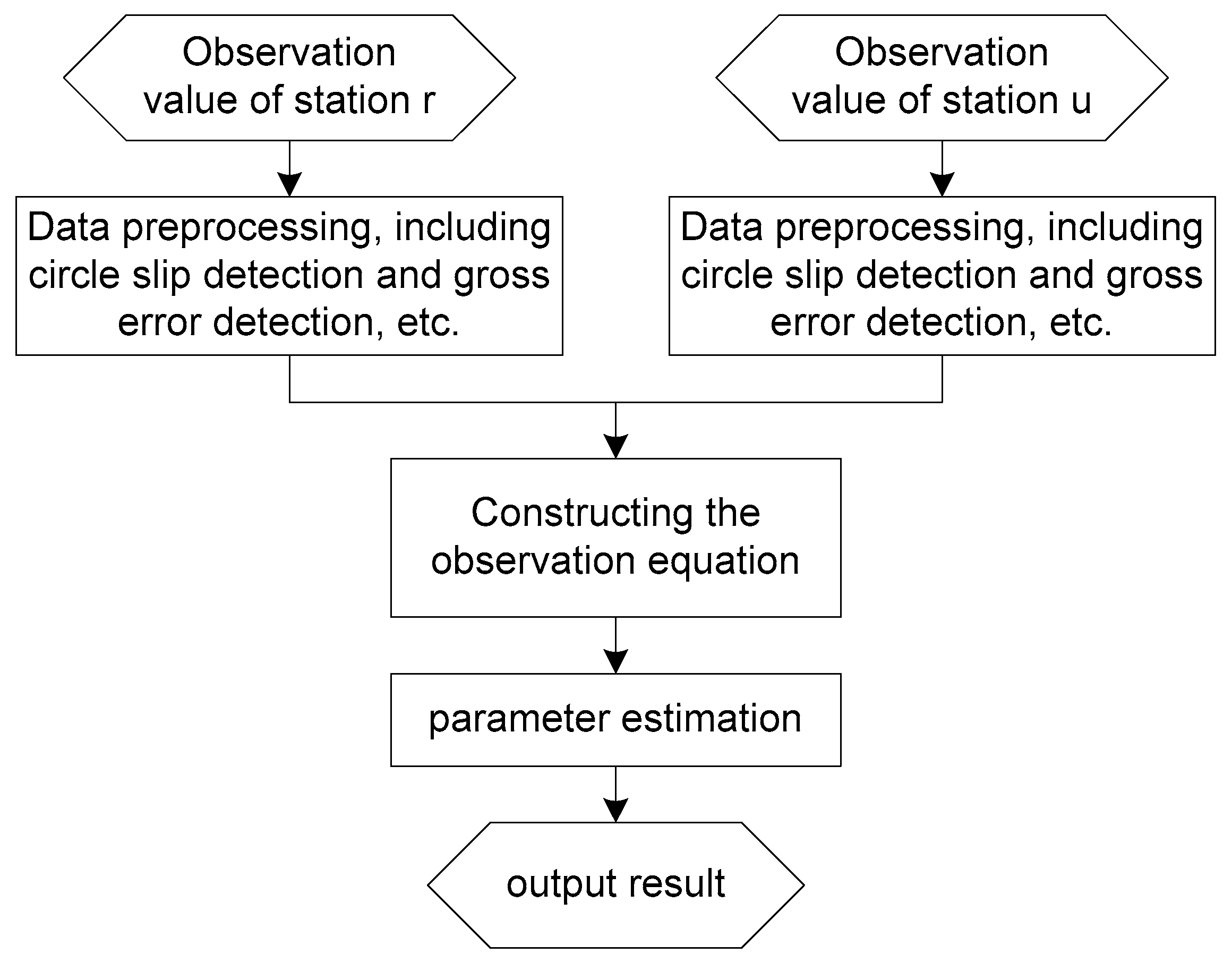
Before constructing the observation equations, we preprocess the observation data from the two stations separately. In the preprocessing stage, we use MW (Melbourne–Wübbena) combinations and ionospheric residuals to detect circle slips and eliminate the satellites with cycle slips. In constructing the observation equations and performing the filter solution, the observations from both stations do not contain cycle slips. The data processing flowchart is shown in Figure 1.
3.2. Experiment 1
In order to verify the time transfer performance of the interstation undifferenced time transfer model, the following experimental scheme is designed based on the satellite orbit and clock offset products released by the IGS Analysis Center.
- Scheme 1:
The two stations in the time link are processed by the traditional PPP model, respectively, and the final satellite orbit and clock offset products are used to carry out the time transfer experiment, which could obtain the clock offset between the two stations relative to the reference time. Then, the receiver clock offset results of the two stations are subtracted to obtain the time transfer results.
- Scheme 2:
Based on the final satellite orbit products, the observation data of the two observation stations in the time link are jointly processed using the interstation undifferenced time transfer model, and one of the observation stations is selected as the reference station to obtain the time transfer results between the two stations.
- Scheme 3:
The satellite orbit and clock offset products adopt the ultrarapid (predicted) products, and the rest of the steps are the same as scheme 1.
- Scheme 4:
The satellite orbit products adopt the ultrarapid (predicted) products, and the rest of the steps are the same as scheme 2.
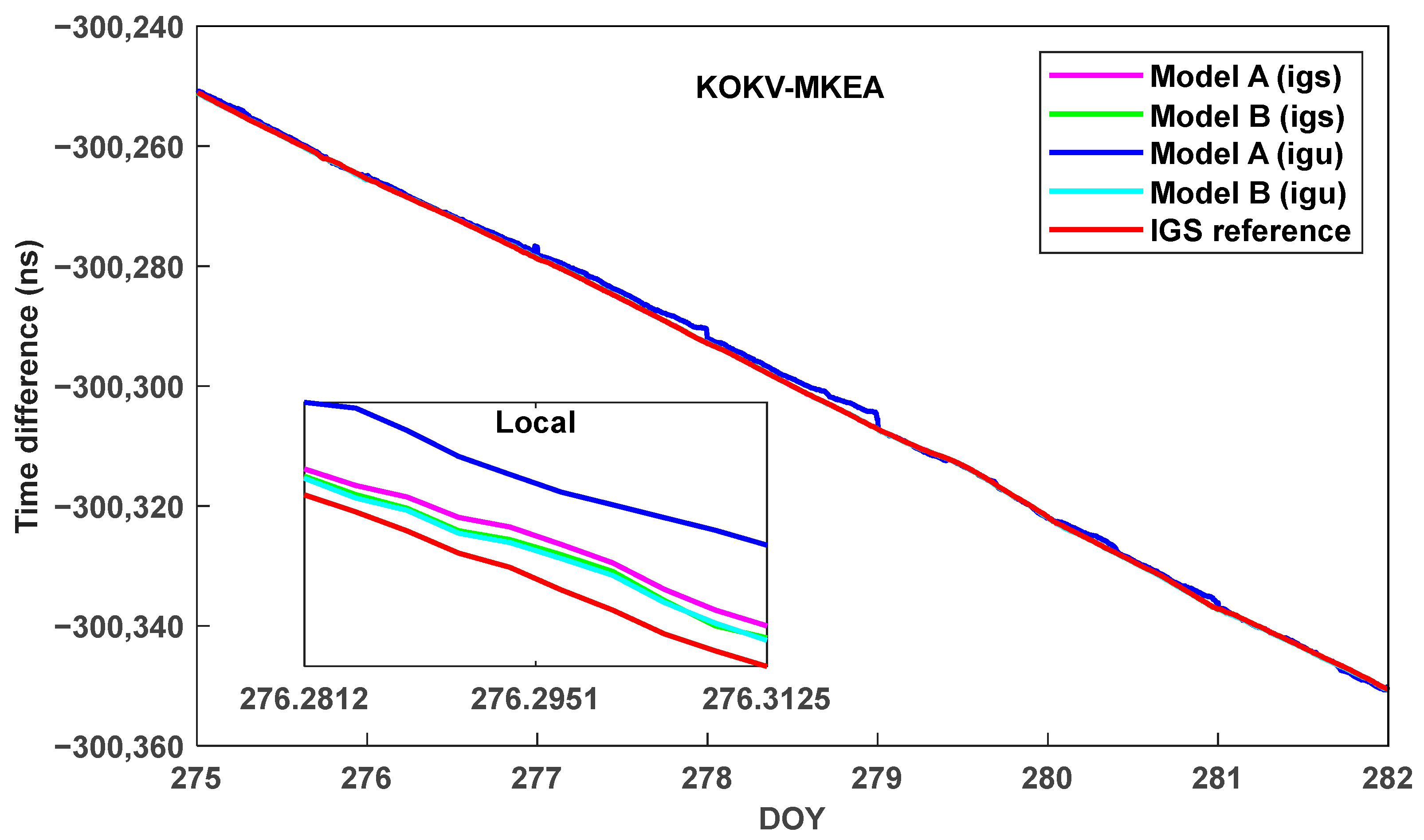
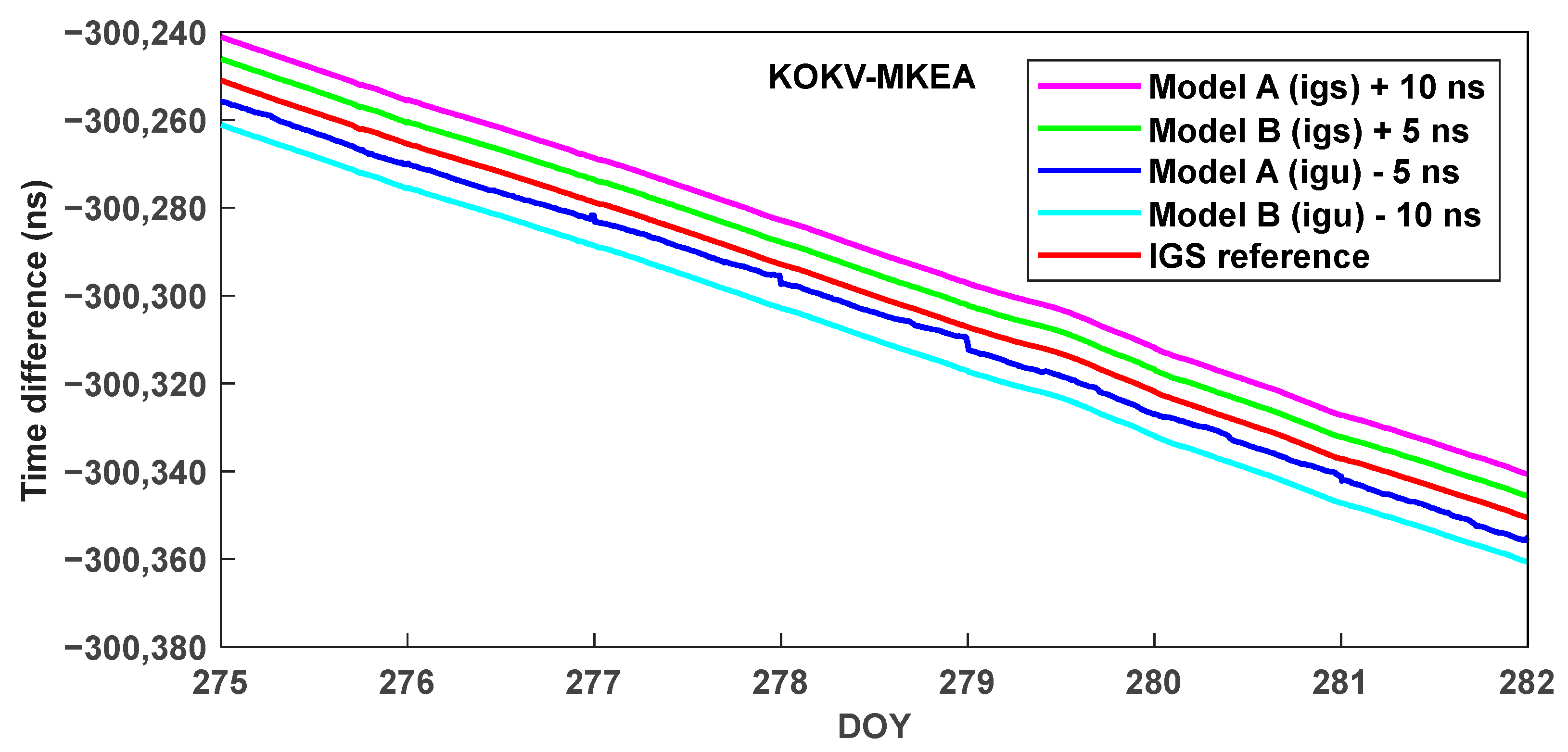
In the experiment, we represent the traditional PPP model as “Model A”, and the interstation undifferenced time transfer model as “Model B”. The accuracy of the clock offset products released by IGS is better than 75 ps, which we use as the “true value” to analyze the time transfer accuracy calculated by the above schemes. Since only the information of two stations in the KOKV-MKEA link can be found in the final clock offset products released by IGS, the KOKV-MKEA link is used for the experiment. Comparing the time transfer results calculated by the above four schemes with the IGS results, their time series are shown in Figure 2. It is worth noting that the sampling interval of the final IGS clock offset products is 5 min, and the solution results need to be downsampled when comparing the accuracy. In order to compare the four time transfer results more clearly, we shifted them by adding 10 ns to the result of scheme 1, adding 5 ns to the result of scheme 2, subtracting 5 ns from the result of scheme 3, and subtracting 10 ns from the result of scheme 4. The shifted time series are then compared with the IGS results, as shown in Figure 3.
It can be seen from Figure 2 that when using the final satellite product, the variation trends of the time transfer results of Model A and Model B are comparable to the results published by IGS. When using ultrarapid (predicted) products, the time transfer results of Model B are closer to the IGS results, while the time transfer results of Model A are significantly worse, and there are many anomalous data in the results. The reason for this is that Model A has to use satellite orbit and clock offset products simultaneously. The ultrarapid (predicted) clock offset products published by IGS have an accuracy of about 3 ns, and the effect on the time transfer result is also several nanoseconds. The partially magnified image in Figure 2 shows that regardless of the satellite product used, the time transfer results of Model B are better than those of Model A, indicating that Model B is more applicable. Figure 3 shows the time transfer results after shifting for the four schemes. We can clearly see that the time transfer results of scheme 3 are poor, while the time transfer results of the other three schemes are in good agreement with the IGS results, and the change trends show consistency, which verifies the feasibility of the interstation undifferenced time transfer model in time transfer.
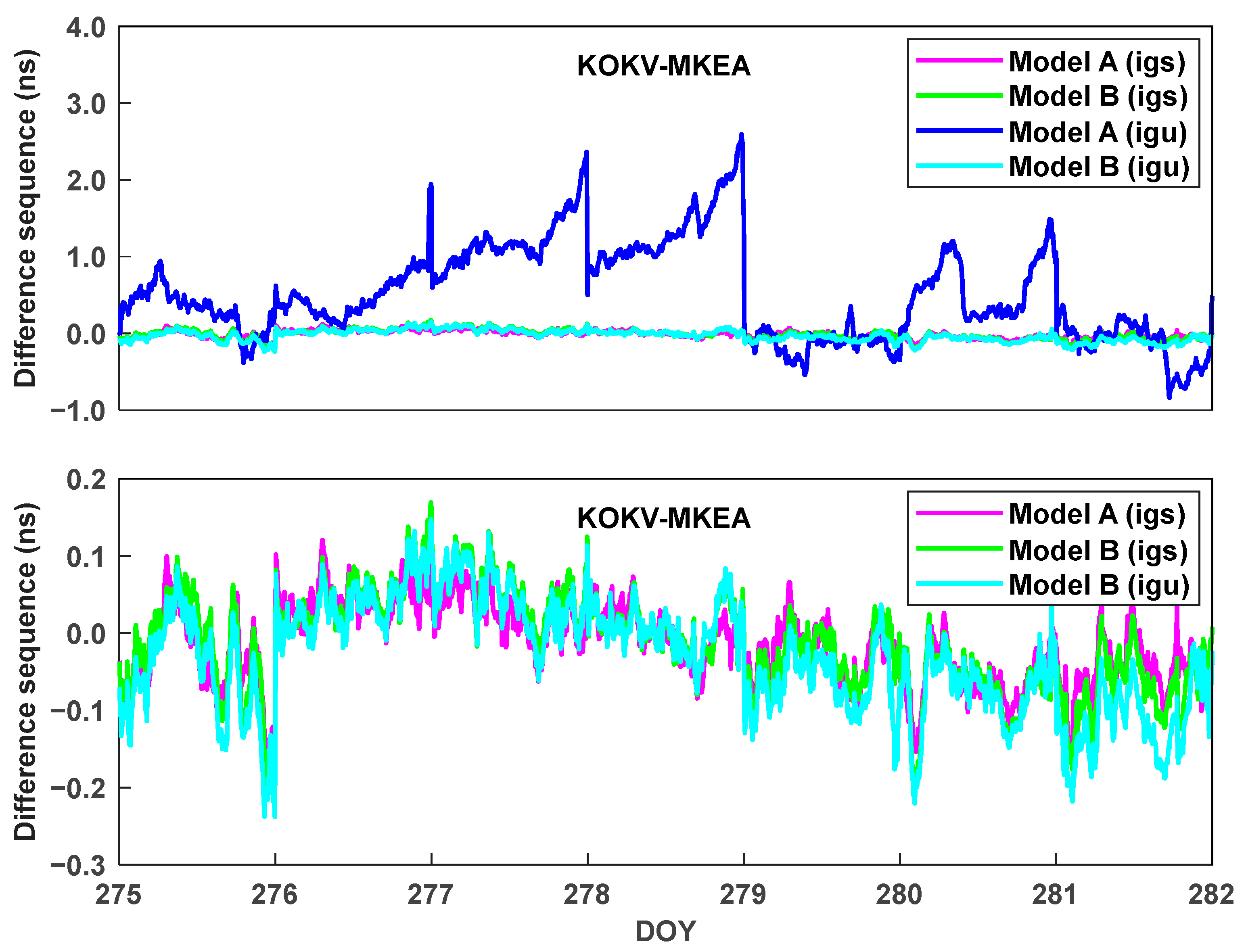
In order to compare the time transfer accuracy of the four schemes and further analyze the time transfer performance of the two models, the time transfer results are compared with the IGS reference value to obtain the time transfer result error series for the four schemes, as shown in Figure 4. The time transfer accuracy is obtained according to the time transfer error series of the four schemes, and the statistical results are shown in Table 4.
As can be seen from Figure 4, except for the blue curve (the time transfer error series obtained by Model A using ultrarapid (predicted) products), the other three curves all fluctuate around the value of 0, which also proves that the time transfer results of these three schemes are consistent with the IGS reference value. In order to better observe the time transfer error series of the remaining three schemes, we delete the blue curves and keep only the remaining three curves. Figure 4 shows that the time transfer error series obtained by the other three schemes all fluctuate at the sub-nanosecond level and are relatively stable overall. As can be seen from Table 4, when ultrarapid (predicted) products are used, the time transfer accuracy of Model A is the worst. The reason is that Model A has to use satellite orbit and satellite clock offset products simultaneously, and the time transfer accuracy is affected by the accuracy of the clock offset products. However, Model B can achieve the same level of accuracy as scheme 1, whether using the final or the ultrarapid (predicted) products, because Model B does not require satellite clock offset products to achieve time transfer. Model A has the highest accuracy of time transfer when using the final satellite products because the accuracy of the final satellite clock offset products is better than 75 ps, so Model A will improve the time transfer accuracy after being corrected by using the clock offset products. The mean, RMS, and STD of the time transfer results of scheme 2 and scheme 4 are not much different from those of scheme 1, with a maximum difference of 0.025 ns. The accuracy of the two schemes is roughly the same, which also explains the feasibility of Model B to a certain extent.
Frequency stability is one of the important indicators to evaluate the accuracy of the time transfer. We use the modified Allan deviation (MDEV) to calculate the frequency stability of the KOKV-MEKA time link under the four schemes, and the sampling interval is 30 s. The results are shown in Figure 5.
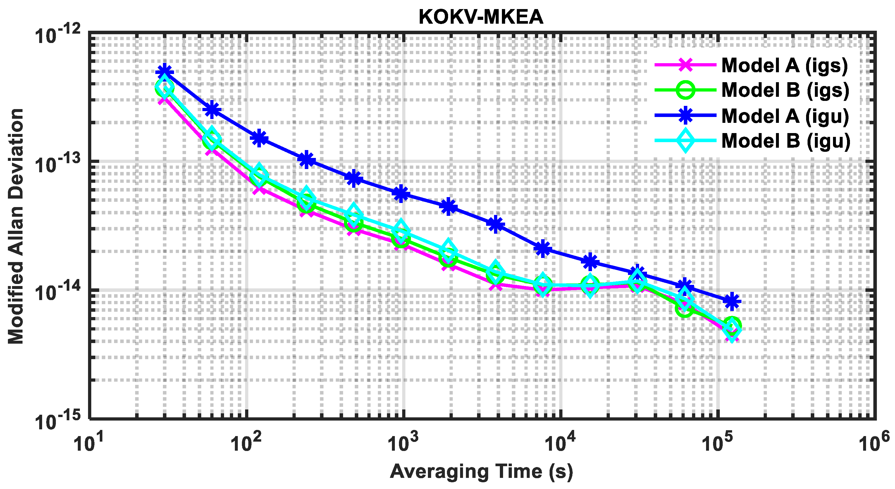
As can be seen from Figure 5, for Model A, the frequency stability of the KOKV-MEKA link is the worst when using the ultrarapid (predicted) products, and the frequency stability is the best when using the final products. The main reason for this is the accuracy and stability of the clock offset products used. For Model B, regardless of which satellite product is used, its frequency stability is consistent with the changing trend of Model A when using the final product, reflecting the better applicability of Model B. When using the final satellite products, the frequency stability for an averaging time at 61,400 s with Model B is 7.24 × 10⁻¹⁵, which is better than that of 7.85 × 10⁻¹⁵ obtained by Model A, indicating that in the postprocessing mode, the long-term stability of the solution results of Model B is equivalent to or even better than that of Model A.
Although Model A will obtain higher-precision time transfer results when using the final satellite products, the acquisition time of the final satellite products is more than one month, which can only be used for postprocessing. The IGS ultrarapid (predicted) satellite products can meet the requirements of real-time application. However, Model A must use satellite orbit and clock offset products simultaneously. The ultrarapid (predicted) satellite clock offset products with 3 ns accuracy can affect the time transfer accuracy by several nanoseconds, so this product is not suitable for Model A. Model B does not require satellite clock offset products and can realize time transfer only by using satellite orbit products. Therefore, Model B has the capability of high-precision real-time time transfer.
3.3. Experiment 2
In order to further analyze the real-time time transfer performance of the two models, based on the observation data from five observation stations (USN7, USN8, APM7, APM8, and APM9), we only use the ultrarapid (predicted) satellite products released by the IGS Analysis Center to conduct experiments. In the experiment, USN7-USN8 and APM7-APM8 are zero baselines, and APM7-APM9 are short baselines. Figure 6 and Figure 7 show the time difference in the three links obtained by the two models. The STD of the time difference corresponding to the two models is given in Table 5.
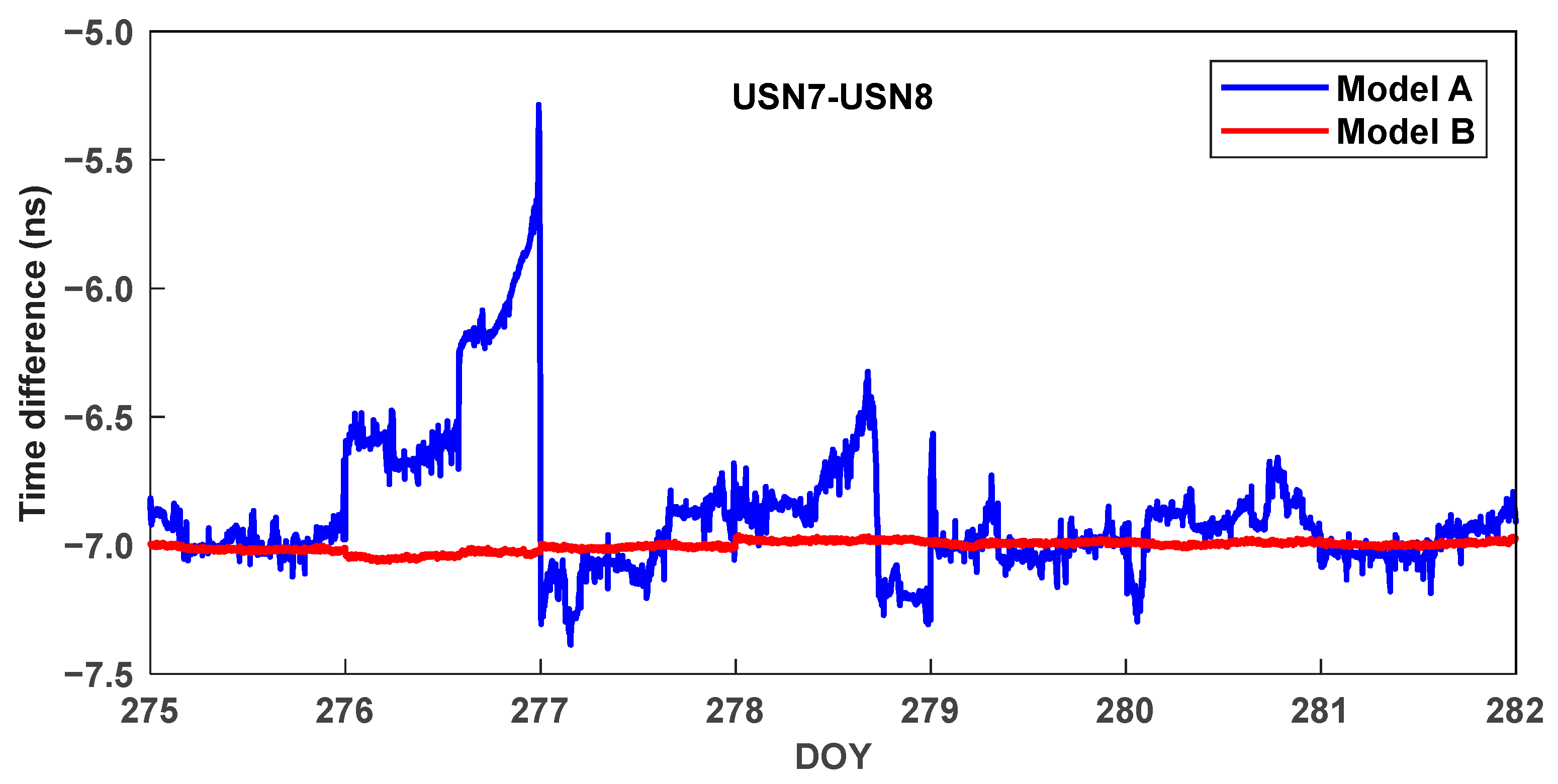
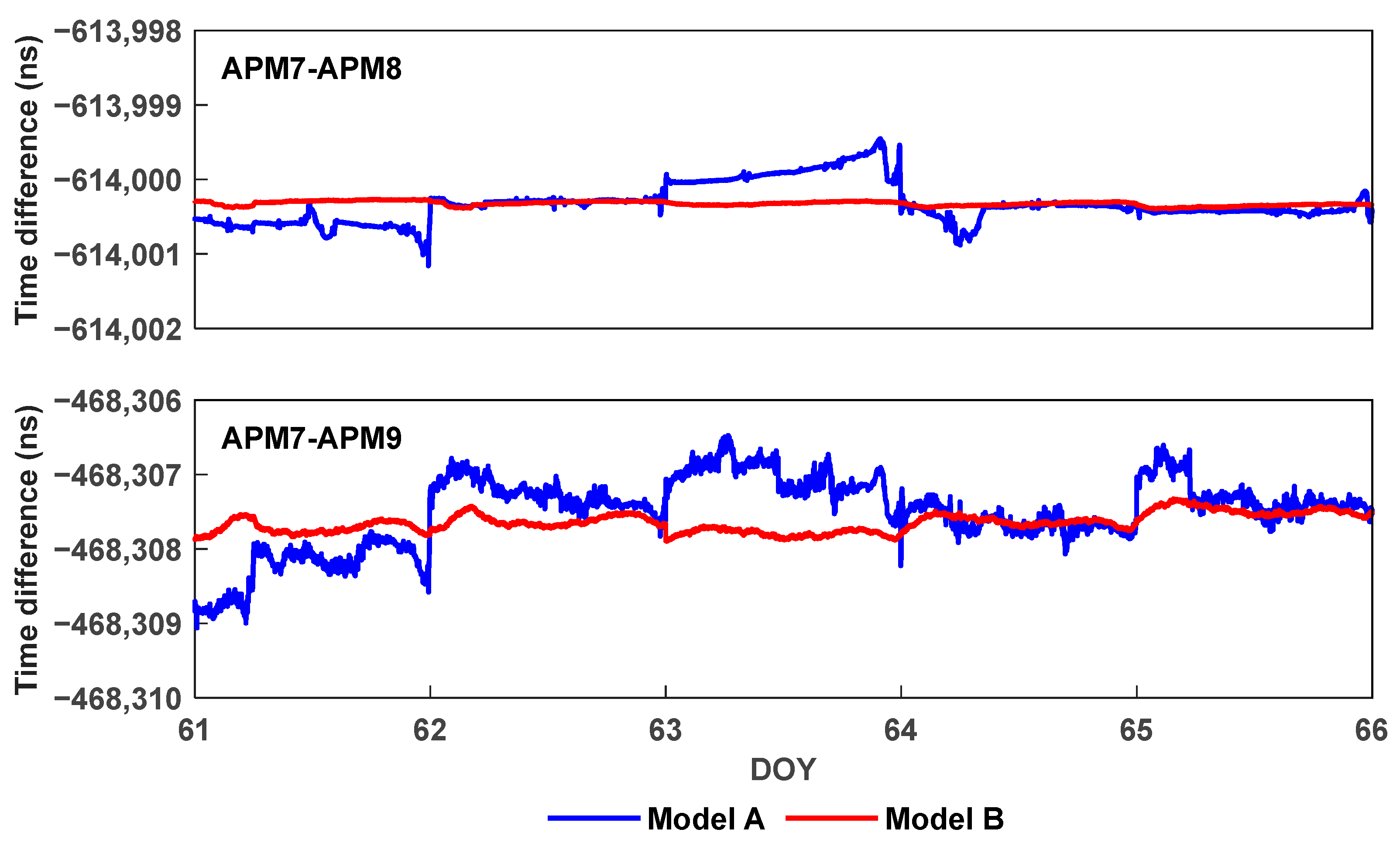
Figure 6 and Figure 7 show the time difference obtained by the two models processing the three time links. Overall, the time difference curve obtained by Model B is more stable than that of Model A, reflecting that Model B has a higher performance in real-time time transfer. The stations USN7 and USN8 use the same antenna and are connected to the same H-maser clock. The stations APM7 and APM8 have the same type of receiver, which is connected to the same antenna and the same Cs clock. Therefore, the time difference between the two time links, USN7-USN8 and APM7-APM8, remains theoretically unchanged, and the processing of these two links can better reflect the time transfer performance of the model. In the APM7-APM9 time link, two receivers are connected to the same Cs clock, but the types of the two receivers and the types of antennas connected are different, which also affects the accuracy of the time transfer, so the time difference curve in the lower figure in Figure 7 is not as stable as in the upper figure. It can be seen from Table 5 that when Model B is used, the STD of the time transfer results of the three time links is better than that of Model A, and the improvement of the time links of the two zero baselines is the most obvious, which can be increased by more than 90%. Due to the influence of receiver type and antenna type, the time transfer accuracy of the APM7-APM9 time link is relatively small, but it can also reach 74.5%.
The modified Allan deviation (MDEV) is used to calculate the frequency stability of the three time links, with a sampling interval of 30 s. The results are shown in Figure 8 and Figure 9.
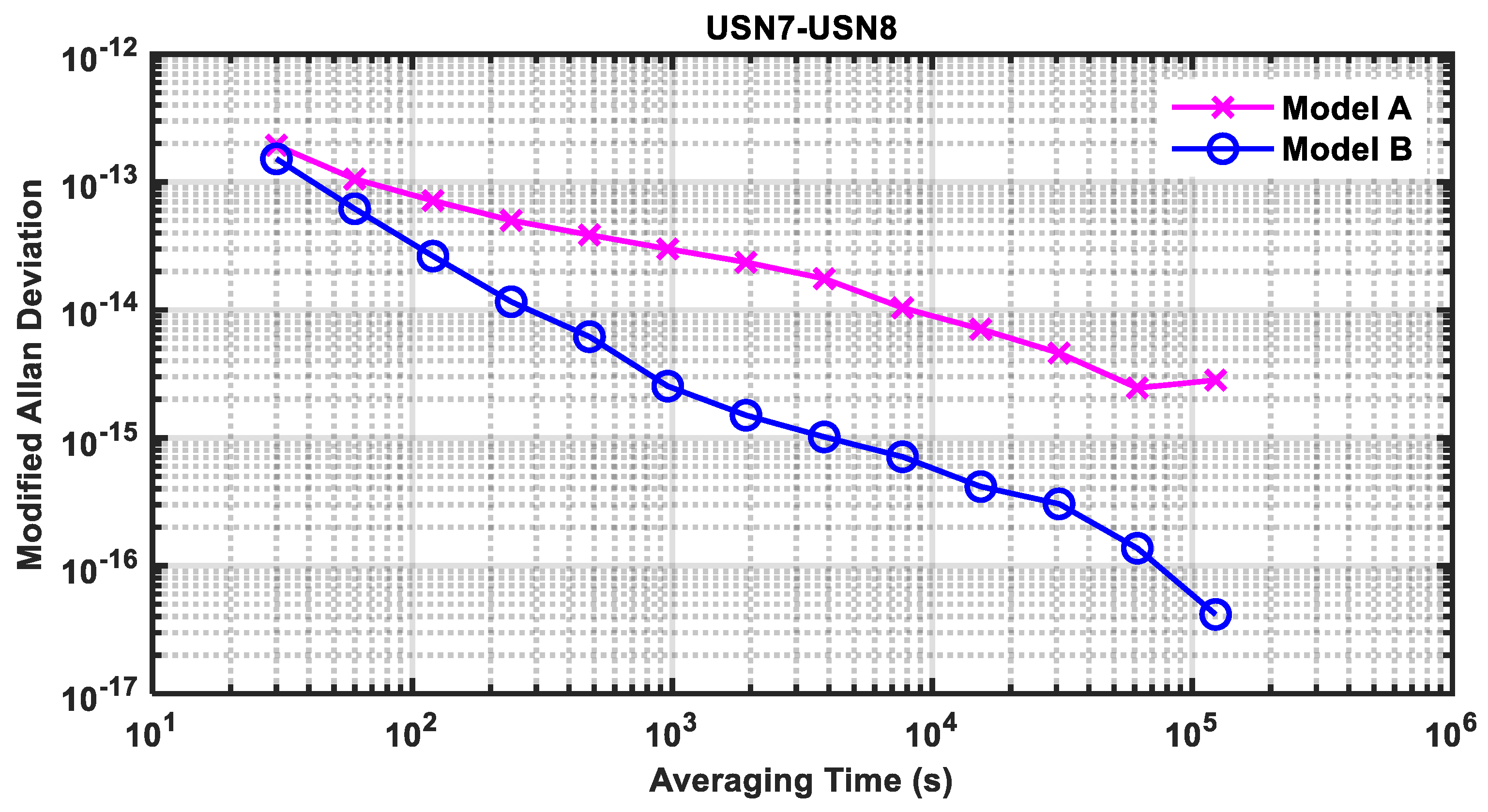
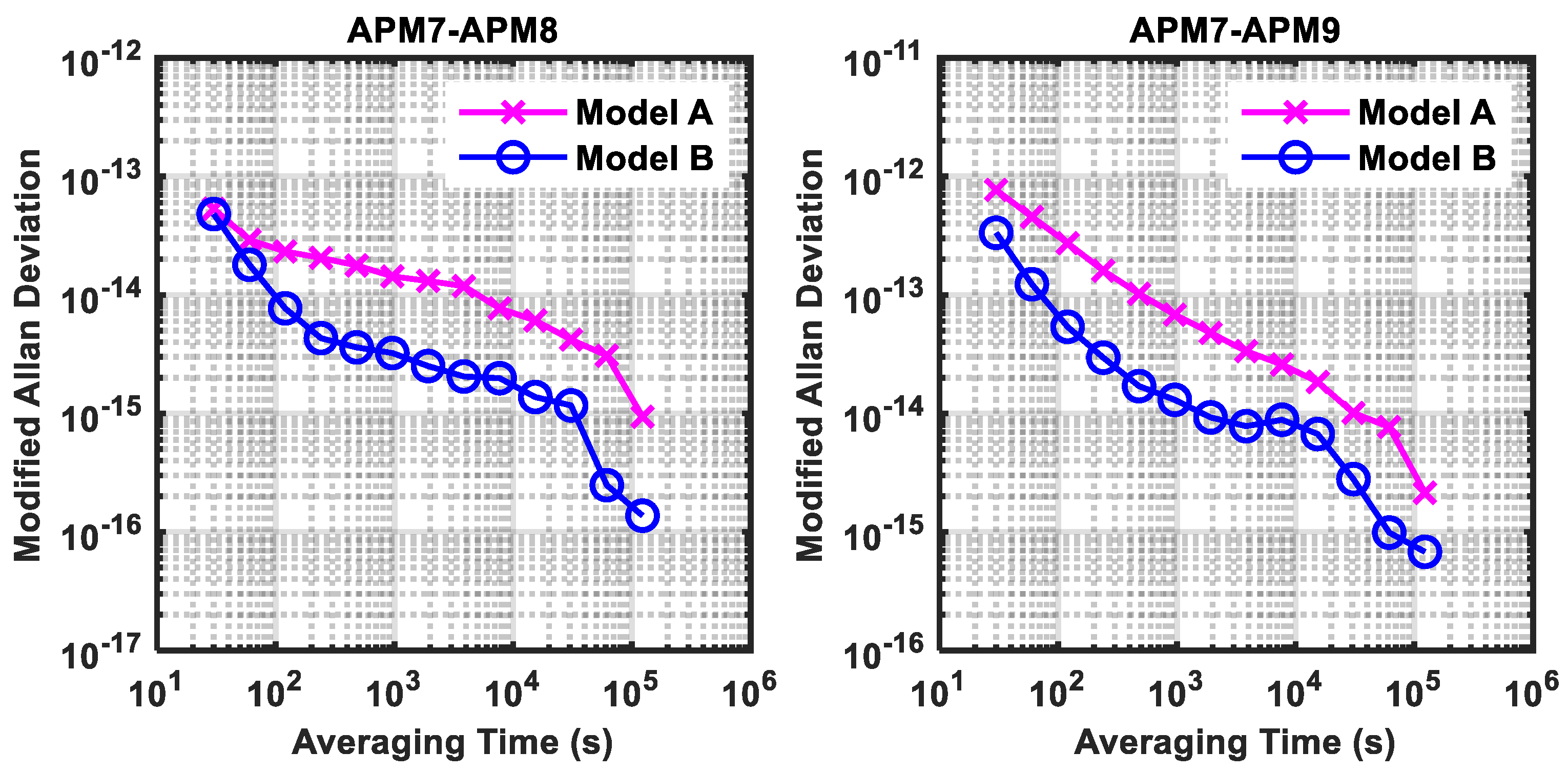
It can be seen in Figure 5, Figure 8 and Figure 9 that the frequency stability of the four time links calculated by Model B is better than that of Model A in real-time time transfer, which can be improved by up to one or even two orders of magnitude, reflecting the good performance of Model B in real-time time transfer. As Model B estimates satellite clock offset parameters synchronously, it is not affected by the quality of the satellite clock offset products in time transfer, so Model B can obtain time transfer results with higher performance. Taking the average time of 122,880 s as an example, the frequency stability of the two models processing the USN7-USN8 time link is 2.82 × 10⁻¹⁵ and 4.16 × 10⁻¹⁷, respectively. The frequency stability of the APM7-APM8 time link is 9.39 × 10⁻¹⁶ and 1.37 × 10⁻¹⁶, respectively. The frequency stability of the APM7-APM9 time link is 2.14 × 10⁻¹⁵ and 6.79 × 10⁻¹⁶, respectively. Compared with Model A, the frequency stability of Model B can be increased by up to 98.5%. By counting the statistics of the frequency stability of the three time links under different average times, the frequency stability of Model B is improved by about 75% on average compared with Model A, which shows the advantage of estimating the satellite clock offset as an unknown parameter.
In real-time time transfer, the accuracy of the real-time satellite clock error is affected by many factors that seriously affect the accuracy and stability of time transfer. Compared with Model A, the advantage of Model B is that the satellite clock offset is used as an unknown parameter to participate in the estimation, which avoids the influence of satellite clock offset products on the time transfer results.
3.4. Experiment 3
In the above experiments, the receiver clock offsets of the two models are estimated as white noise, the clock offset parameter of adjacent epochs is independent of each other, and the receiver clock offset will absorb some of the error model residuals and other noise. The atomic clock has high-frequency stability, and the receiver clock offsets of adjacent epochs have strong autocorrelation. Therefore, the accuracy and stability of time transfer can be effectively improved by constructing the receiver clock offset constraint model. In this experiment, considering the correlation of receiver clock offsets of adjacent epochs, we combine the interstation undifferenced time transfer model and the receiver clock offset constraint model to perform time transfer and design the following two experimental schemes:
Scheme 1: Estimate the receiver clock offset using the white noise model.
Scheme 2: Estimate the receiver clock offset using the clock offset-constrained model. The corresponding modified Allan deviation (MDEV) is obtained using the time differences of the previous day, and then the prior noise variance of the receiver clock offset parameter in the interstation undifferenced time transfer model is determined according to Equation (6).
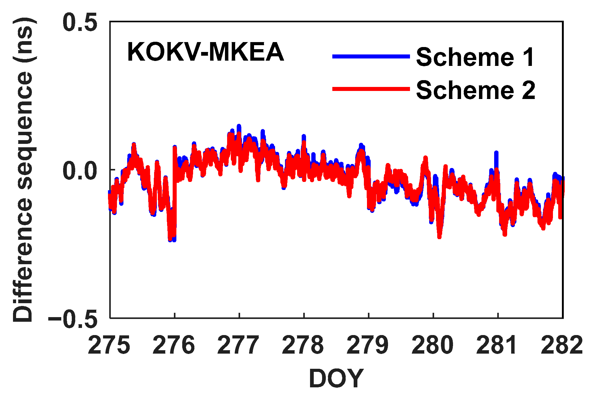
Experiments were carried out using the KOKV-MKEA, USN7-USN8, APM7-APM8, and APM7-APM9 time links, in which the accuracy and stability of the time transfer obtained from the white noise model and the receiver clock offset constraint model were compared. Using the IGS final products to analyze the time transfer accuracy of the KOKV-MKEA time link, Figure 10 shows the error sequences of the time transfer results obtained by the two schemes, and the time transfer accuracy of the two schemes is listed in Table 6.
Figure 10 shows the time transfer error sequences obtained for the two schemes compared with the IGS final products. Overall, the two error curves fluctuate around the value of 0, indicating that the clock offset sequences obtained by the two clock offset calculation models are in good agreement with the IGS final products. In Figure 10, we can see that the results using the clock offset constraint model are less noisy than the white noise model. It can be seen from Table 6 that the RMS values of the two schemes are the same, and the STD value of scheme 2 is slightly better than that of scheme 1, proving the feasibility of our model in time transfer.
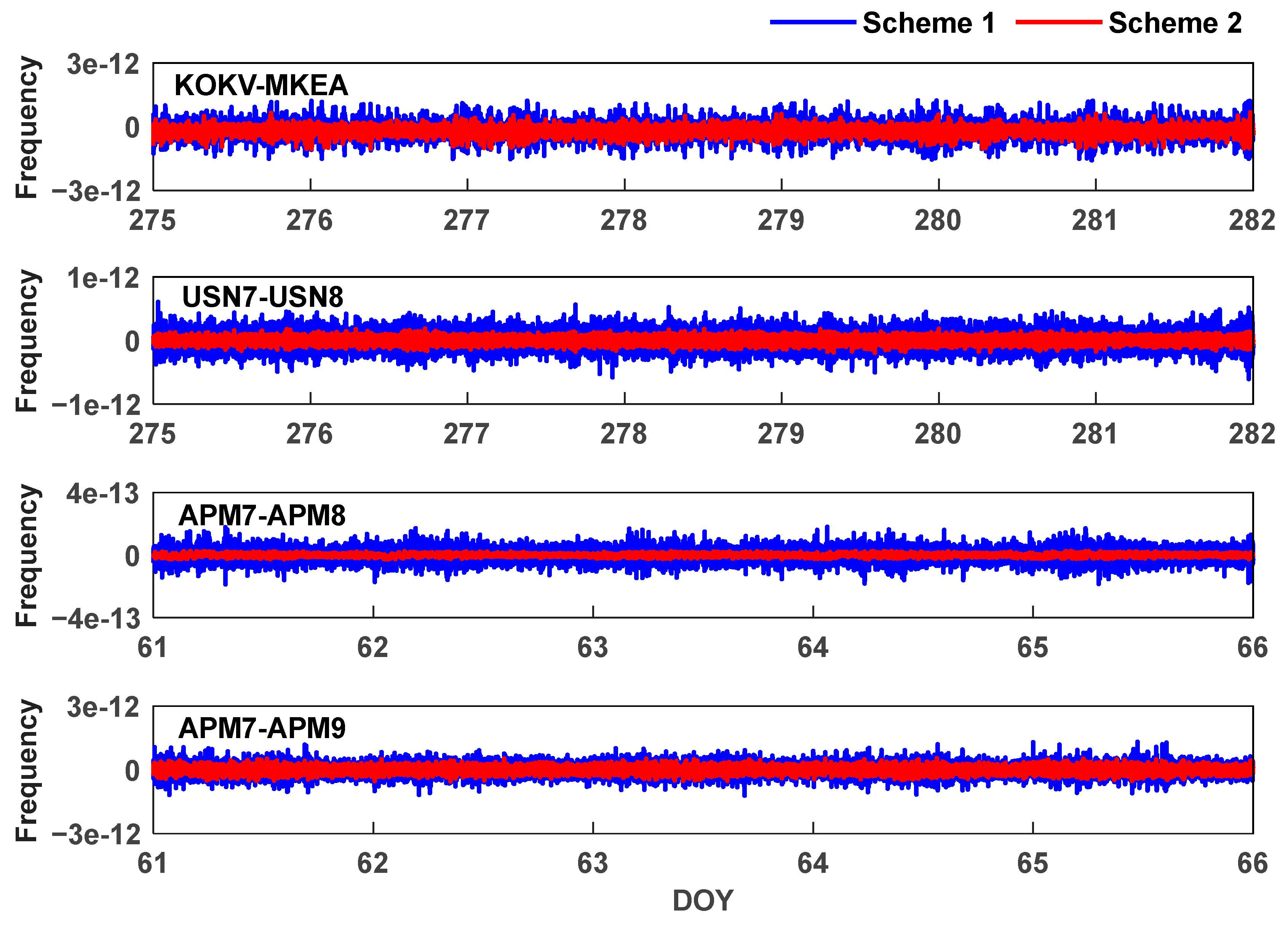
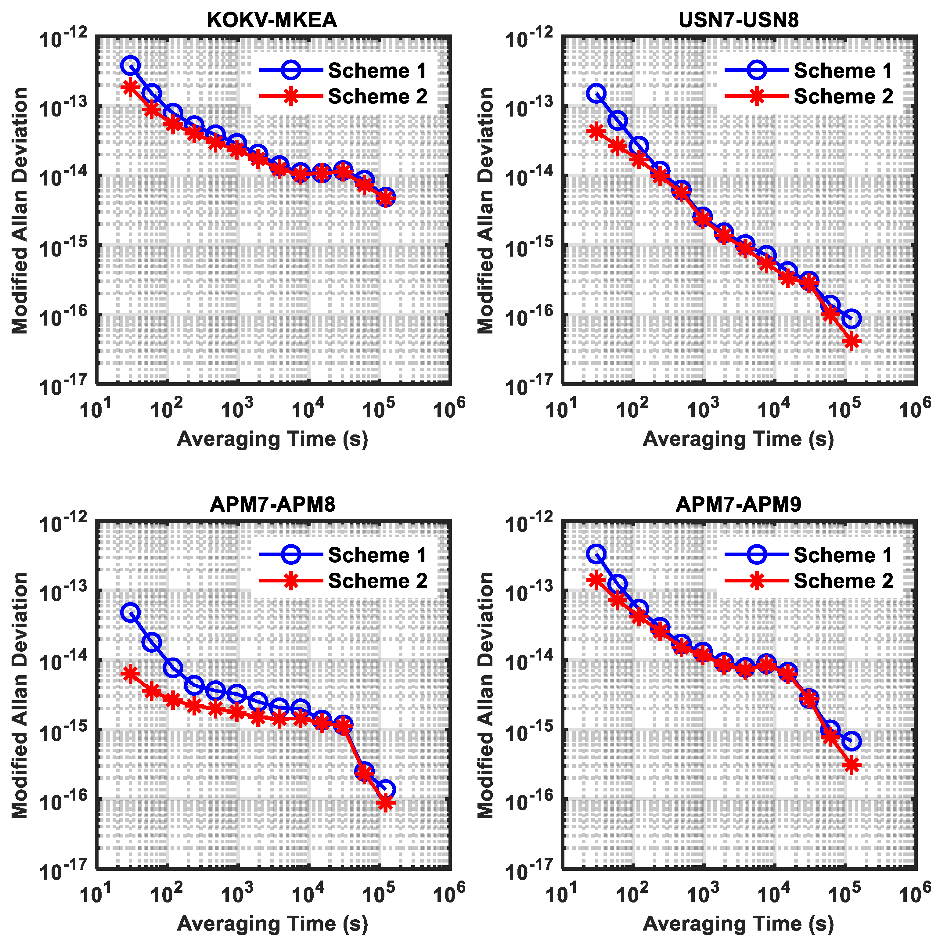
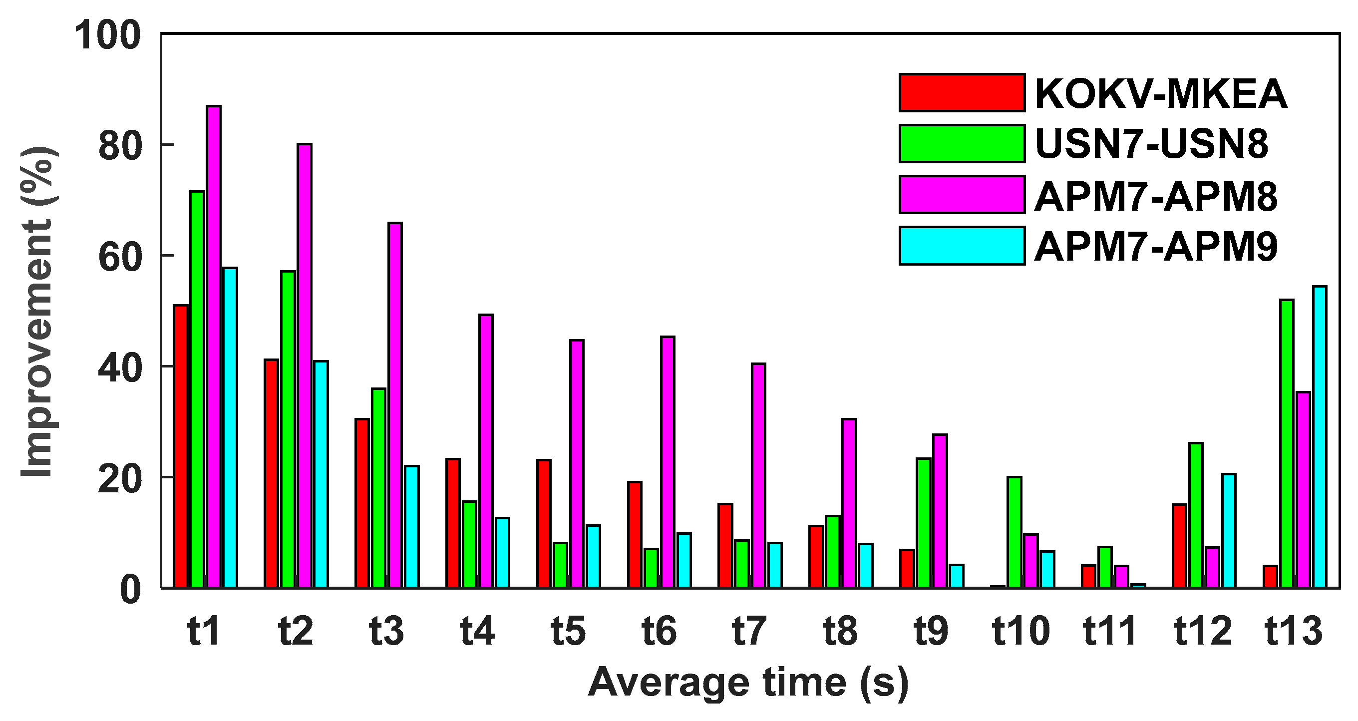
To further evaluate the time transfer performance of the two schemes, the time transfer results of the four time links are analyzed. We use the clock offset sequences to obtain the corresponding frequency sequence. For the convenience of analysis, we remove the gross error, and the frequency sequences after removing the gross error are shown in Figure 11. Since only the “true value” of the time transfer results for the KOKV-MKEA time link can be found in the IGS final products, the frequency stability is used to evaluate the time transfer performance when analyzing the four time links. Figure 12 shows the MDEV for the four time links. Compared with scheme 1, the frequency stability of scheme 2 has improved to some extent at different average times, with the short-term stability improvement being the most obvious. To obtain a clearer picture of the improvement in frequency stability, we calculated the improvement for the four time links, and the results are shown in Figure 13.
In Figure 11, the blue line is the frequency sequence obtained by the traditional white noise model (scheme 1), and the red line is the frequency sequence obtained by the receiver clock offset constraint model (scheme 2). Among the four time links, the time transfer frequency sequences obtained by scheme 2 have less noise than those of scheme 1, indicating that scheme 2 can obtain time transfer results with higher stability. As can be seen from Figure 12, the frequency stability of the four time links obtained by scheme 2 is better than that of scheme 1, with the most significant improvement in terms of short-term stability. Taking the average time of 30 s as an example, the frequency stability of the KOKV-MKEA time link processed by the two clock offset models is 3.81 × 10⁻¹³ and 1.86 × 10⁻¹³, respectively. The frequency stability of the USN7-USN8 time link is 1.52 × 10⁻¹³ and 4.32 × 10⁻¹⁴, respectively. The frequency stability of the APM7-APM8 time link is 4.81 × 10⁻¹⁴ and 6.31 × 10⁻¹⁵, respectively. The frequency stability of the APM7-APM9 time link is 3.35 × 10⁻¹³ and 1.41 × 10⁻¹³, respectively. Compared with scheme 1, the MDEVs of the four time links using scheme 2 are increased by 51.0%, 71.5%, 86.9%, and 57.8%, respectively. In terms of long-term stability, when the average time is 122,880 s, the frequency stabilities of the four time links using two schemes are 4.88 × 10⁻¹⁵, 8.66 × 10⁻¹⁷, 1.37 × 10⁻¹⁶, and 6.79 × 10⁻¹⁶ and 4.69 × 10⁻¹⁵, 4.16 × 10⁻¹⁷, 8.87 × 10⁻¹⁷, and 3.09 × 10⁻¹⁶, respectively, proving the superiority of the clock offset constraint model in time transfer.
To obtain a clearer picture of the improvement of the clock offset constraint model compared with the white noise model, we calculated the improvement percentages of the four time links at different average times and plotted them as histograms for easy analysis. As can be seen from Figure 13, the frequency stability of the four time links was improved, especially the short-term stability, which can be increased by 86.9% at the highest. We speculate that the main reason is that the clock offset noise obtained by the clock offset constraint model is much lower than that obtained by the white noise model (see Figure 11).
From the above experiments, it can be seen that in the real-time processing mode, the interstation undifferenced real-time time transfer method with refined modeling of the receiver clock can achieve higher performance time transfer results for the following two reasons: One reason is that the satellite clock offset is estimated as the unknown parameter in the interstation undifferenced time transfer model, and the accuracy and stability of the time transfer are not affected by the satellite clock offset products. Another reason is that the clock offset constraint model takes into account the correlation of the receiver clock offset in previous and subsequent epochs, which can effectively reduce the noise in the clock offset estimation and improve the stability and accuracy of the time transfer. In summary, the interstation undifferenced real-time time transfer method with refined modeling of the receiver clock has greater advantages in real-time time transfer compared with traditional time transfer schemes.
4. Discussion
The premise of the PPP method to obtain high-precision time transfer results is to use high-precision satellite orbit and clock offset products at the same time. However, in real-time processing, satellite clocks are difficult to accurately forecast due to their own characteristics, so real-time satellite clock offset products have low accuracy, which makes it difficult to meet the needs of high-precision time transfer. And the receiver clock offset is often estimated by the white noise model, which ignores the correlation of clock offset between adjacent epochs and affects the accuracy and stability of time transfer.
In this paper, we proposed a new time transfer method that requires only satellite orbit products and effectively reduces noise in clock offset estimation by using a clock offset constraint model. The experimental results show that compared with the traditional time transfer model, the accuracy and stability of time transfer are improved by more than 70% and 60%, respectively. In both real-time and postevent scenarios, this method can obtain better time transfer results and has the capability of sub-nanosecond time transfer.
Atomic clocks are easily affected by internal factors and external environments, and their pattern of change is difficult to accurately describe. In addition to the trend terms, atomic clocks are also affected by periodic and random terms, and the noise of different types of atomic clocks is not the same. Therefore, we will next analyze the data of different types of atomic clocks and construct their respective clock offset constraint models for different types of atomic clocks to further improve time transfer performance.
5. Conclusions
The continuity and stability of PPP time transfer will be seriously affected when there is a network communication failure that makes the real-time satellite clock offset products unavailable. In addition, the receiver clock offset is often estimated using the white noise model, which ignores the correlation of the clock offsets between adjacent epochs and the stability of the atomic clock itself. In this contribution, we proposed an interstation undifferenced real-time time transfer method with refined modeling of the receiver clock, where the satellite clock offset and the receiver clock offset are both used as parameters to be estimated, and the receiver clock offset estimates are based on the clock offset constraint model instead of the white noise model.
Using data from IGS observatories and self-collected data, we evaluated the time transfer performance of the proposed method. The experimental results showed that the real-time time transfer accuracy of the interstation undifferenced time transfer model is equivalent to the postevent time transfer accuracy, both of which can reach sub-nanosecond accuracy. Based on IGS ultra-rapid (predicted) products, the time transfer results obtained by the interstation undifferenced time transfer model are more stable than the traditional PPP model, and the time transfer accuracy of the four time links has increased by 88.4%, 92.9%, 88.6%, and 74.5%, respectively. Compared with the traditional PPP model, the frequency stability calculated by the interstation undifferenced time transfer model can be improved by up to two orders of magnitude, and frequency stability on the order of 10–16 can be achieved at the average time of day. In addition, compared with the white noise model, the time transfer results of the four time links after applying the receiver clock offset constraint model are less noisy, and the frequency stability is improved to varying degrees. Among them, the short-term stability improvement is significant, with a maximum of 86.9% and an average improvement of approximately 66.8%.
The interstation undifferenced real-time time transfer method with refined modeling of the receiver clock avoids the influence of external satellite clock offset products, which ensures the performance of the real-time time transfer. Moreover, the method uses the clock offset constraint model to estimate the receiver clock offset, which can effectively reduce the noise of the clock offset estimation and further improve the stability and accuracy of time transfer. Therefore, the proposed method has the capability of real-time sub-nanosecond time transfer.
Author Contributions
Conceptualization, D.L.; data curation, D.L. and M.L.; formal analysis, D.L. and G.L.; funding acquisition, G.L.; methodology, D.L.; project administration, G.L.; software, D.L.; supervision, G.L.; validation, W.Z. and W.L.; writing—original draft, D.L.; writing—review and editing, D.L., G.L., W.Z., W.L., B.Z. and M.L. All authors have read and agreed to the published version of the manuscript.
Funding
This work is funded by the Project Supported by the Open Fund of Hubei Luojia Laboratory (Grant No. 220100044), the National Natural Science Foundation of China (Grant No. 41774017) and the National Key Research Programme of China Collaborative Precision Positioning Project (Grant No. 2016YFB0501900).
Data Availability Statement
IGS observation data, satellite orbit and clock offset products are downloaded from the CDDIS (https://cddis.nasa.gov). Self-collected datasets are available from the corresponding author upon reasonable request.
Acknowledgments
We would like to thank the IGS for providing related satellite products and GNSS data.
Conflicts of Interest
The authors declare no conflict of interest.
References
- Milner, W.R.; Robinson, J.M.; Kennedy, C.J.; Bothwell, T.; Kedar, D.; Matei, D.G.; Legero, T.; Sterr, U.; Riehle, F.; Leopardi, H.; et al. Demonstration of a Timescale Based on a Stable Optical Carrier. Phys. Rev. Lett. 2019, 123, 173201. [Google Scholar] [CrossRef] [PubMed]
- Roberts, B.M.; Blewitt, G.; Dailey, C.; Murphy, M.; Pospelov, M.; Rollings, A.; Sherman, J.; Williams, W.; Derevianko, A. Search for Domain Wall Dark Matter with Atomic Clocks on Board Global Positioning System Satellites. Nat. Commun. 2017, 8, 1195. [Google Scholar] [CrossRef] [PubMed]
- Mi, X.; Zhang, B.; El-Mowafy, A.; Wang, K.; Yuan, Y. On the Potential of Undifferenced and Uncombined GNSS Time and Frequency Transfer with Integer Ambiguity Resolution and Satellite Clocks Estimated. GPS Solut. 2022, 27, 25. [Google Scholar] [CrossRef]
- Jiang, Z.; Czubla, A.; Nawrocki, J.; Lewandowski, W.; Arias, E.F. Comparing a GPS Time Link Calibration with an Optical Fibre Self-Calibration with 200 Ps Accuracy. Metrologia 2015, 52, 384. [Google Scholar] [CrossRef]
- Jiang, Z.; Zhang, V.; Huang, Y.-J.; Achkar, J.; Piester, D.; Lin, S.-Y.; Wu, W.; Naumov, A.; Yang, S.; Nawrocki, J.; et al. Use of Software-Defined Radio Receivers in Two-Way Satellite Time and Frequency Transfers for UTC Computation. Metrologia 2018, 55, 685. [Google Scholar] [CrossRef]
- Fujieda, M.; Piester, D.; Gotoh, T.; Becker, J.; Aida, M.; Bauch, A. Carrier-Phase Two-Way Satellite Frequency Transfer over a Very Long Baseline. Metrologia 2014, 51, 253. [Google Scholar] [CrossRef]
- Zhao, W.; Liu, G.; Gao, M.; Zhang, B.; Hu, S.; Lyu, M. A New Inter-System Double-Difference RTK Model Applicable to Both Overlapping and Non-Overlapping Signal Frequencies. Satell. Navig. 2023, 4, 22. [Google Scholar] [CrossRef]
- Pei, G.; Pan, L.; Zhang, Z.; Yu, W. GNSS/RNSS Integrated PPP Time Transfer: Performance with Almost Fully Deployed Multiple Constellations and a Priori ISB Constraints Considering Satellite Clock Datums. Remote Sens. 2023, 15, 2613. [Google Scholar] [CrossRef]
- Petit, G. Sub-10-16 Accuracy GNSS Frequency Transfer with IPPP. GPS Solut. 2021, 25, 22. [Google Scholar] [CrossRef]
- Yuanxi, Y. Resilient PNT Concept Frame. Acta Geod. Cartogr. Sin. 2018, 47, 893–898. [Google Scholar]
- Harmegnies, A.; Defraigne, P.; Petit, G. Combining GPS and GLONASS in All-in-View for Time Transfer. Metrologia 2013, 50, 277. [Google Scholar] [CrossRef]
- Wang, S.; Zhao, X.; Ge, Y.; Yang, X. Investigation of Real-Time Carrier Phase Time Transfer Using Current Multi-Constellations. Measurement 2020, 166, 108237. [Google Scholar] [CrossRef]
- Wei, P.; Yang, C.; Yang, X.; Cao, F.; Hu, Z.; Li, Z.; Guo, J.; Li, X.; Qin, W. Common-View Time Transfer Using Geostationary Satellite. IEEE Trans. Ultrason. Ferroelectr. Freq. Control 2020, 67, 1938–1945. [Google Scholar] [CrossRef]
- Zeng, W.; He, L.; Liu, Y. Analysis of Synchronization Performance between Two Stations with Satellite Single-Frequency Close-Range Common View and Dual-Frequency One-Way Timing. J. Time Freq. 2020, 43, 101–112. [Google Scholar]
- Tu, R.; Zhang, P.; Zhang, R.; Liu, J.; Lu, X. Modeling and Performance Analysis of Precise Time Transfer Based on BDS Triple-Frequency Un-Combined Observations. J. Geod. 2019, 93, 837–847. [Google Scholar] [CrossRef]
- Bruyninx, C.; Defraigne, P.; Sleewaegen, J.-M. Time and Frequency Transfer Using GPS Codes and Carrier Phases: Onsite Experiments. GPS Solut. 1999, 3, 1–10. [Google Scholar] [CrossRef]
- Zumberge, J.F.; Heflin, M.B.; Jefferson, D.C.; Watkins, M.M.; Webb, F.H. Precise Point Positioning for the Efficient and Robust Analysis of GPS Data from Large Networks. J. Geophys. Res. Solid Earth 1997, 102, 5005–5017. [Google Scholar] [CrossRef]
- Pireaux, S.; Defraigne, P.; Wauters, L.; Bergeot, N.; Baire, Q.; Bruyninx, C. Higher-Order Ionospheric Effects in GPS Time and Frequency Transfer. GPS Solut. 2010, 14, 267–277. [Google Scholar] [CrossRef]
- Xu, W.; Shen, W.; Cai, C.; Li, L.; Wang, L.; Ning, A.; Shen, Z. Comparison and Evaluation of Carrier Phase PPP and Single Difference Time Transfer with Multi-GNSS Ambiguity Resolution. GPS Solut. 2022, 26, 58. [Google Scholar] [CrossRef]
- Defraigne, P.; Aerts, W.; Harmegnies, A.; Petit, G.; Rovera, D.; Uhrich, P. Advances in Multi-GNSS Time Transfer. In Proceedings of the 2013 Joint European Frequency and Time Forum & International Frequency Control Symposium (EFTF/IFC), Prague, Czech Republic, 21–25 July 2013; pp. 508–512. [Google Scholar]
- Petit, G.; Jiang, Z. Precise Point Positioning for TAI Computation. In Proceedings of the 2007 IEEE International Frequency Control Symposium Joint with the 21st European Frequency and Time Forum, Geneva, Switzerland, 29 May–1 June 2007; pp. 395–398. [Google Scholar]
- Rose, J.A.R.; Watson, R.J.; Allain, D.J.; Mitchell, C.N. Ionospheric Corrections for GPS Time Transfer. Radio Sci. 2014, 49, 196–206. [Google Scholar] [CrossRef]
- Tavella, P.; Petit, G. Precise Time Scales and Navigation Systems: Mutual Benefits of Timekeeping and Positioning. Satell. Navig. 2020, 1, 10. [Google Scholar] [CrossRef]
- Yao, J.; Skakun, I.; Jiang, Z.; Levine, J. A Detailed Comparison of Two Continuous GPS Carrier-Phase Time Transfer Techniques. Metrologia 2015, 52, 666. [Google Scholar] [CrossRef]
- Beutler, G.; Moore, A.W.; Mueller, I.I. The International Global Navigation Satellite Systems Service (IGS): Development and Achievements. J. Geod. 2009, 83, 297–307. [Google Scholar] [CrossRef]
- Dow, J.M.; Neilan, R.E.; Rizos, C. The International GNSS Service in a Changing Landscape of Global Navigation Satellite Systems. J. Geod. 2009, 83, 191–198. [Google Scholar] [CrossRef]
- Guo, J.; Geng, J. GPS Satellite Clock Determination in Case of Inter-Frequency Clock Biases for Triple-Frequency Precise Point Positioning. J. Geod. 2018, 92, 1133–1142. [Google Scholar] [CrossRef]
- Petit, G.; Arias, E.F. Use of IGS Products in TAI Applications. J. Geod. 2009, 83, 327–334. [Google Scholar] [CrossRef]
- Teunissen, P.J.G. GNSS Precise Point Positioning. In Position, Navigation, and Timing Technologies in the 21st Century: Integrated Satellite Navigation, Sensor Systems, and Civil Applications; John Wiley & Sons, Inc.: Hoboken, NJ, USA, 2020; pp. 503–528. [Google Scholar] [CrossRef]
- Zhang, X.; Cai, S.; Li, X.; Guo, F. Accuracy Analysis of Time and Frequency Transfer Based on Precise Point Positioning. Geomat. Inf. Sci. Wuhan Univ. 2010, 35, 274–278. [Google Scholar]
- Zhang, P.; Tu, R.; Gao, Y.; Liu, N.; Zhang, R. Evaluation of Carrier-Phase Precise Time and Frequency Transfer Using Different Analysis Centre Products for GNSSs. Meas. Sci. Technol. 2019, 30, 65003. [Google Scholar] [CrossRef]
- Defraigne, P.; Aerts, W.; Pottiaux, E. Monitoring of UTC(k)’s Using PPP and IGS Real-Time Products. GPS Solut. 2015, 19, 165–172. [Google Scholar] [CrossRef]
- Ge, Y.; Cao, X.; Lyu, D.; He, Z.; Ye, F.; Xiao, G.; Shen, F. An Investigation of PPP Time Transfer via BDS-3 PPP-B2b Service. GPS Solut. 2023, 27, 61. [Google Scholar] [CrossRef]
- Liu, G.; Gao, M.; Yin, X.; Xiao, G.; Lv, D.; Wang, S.; Wang, R. High-Precision Cloud Platform Timing Based on GNSS Precise Point Positioning. Acta Geod. Cartogr. Sin. 2022, 51, 1736–1743. [Google Scholar]
- Guo, W.; Song, W.; Niu, X.; Lou, Y.; Gu, S.; Zhang, S.; Shi, C. Foundation and Performance Evaluation of Real-Time GNSS High-Precision One-Way Timing System. GPS Solut. 2019, 23, 23. [Google Scholar] [CrossRef]
- Ge, Y.; Dai, P.; Qin, W.; Yang, X.; Zhou, F.; Wang, S.; Zhao, X. Performance of Multi-GNSS Precise Point Positioning Time and Frequency Transfer with Clock Modeling. Remote Sens. 2019, 11, 347. [Google Scholar] [CrossRef]
- Lou, Y.; Zheng, F.; Gu, S.; Wang, C.; Guo, H.; Feng, Y. Multi-GNSS Precise Point Positioning with Raw Single-Frequency and Dual-Frequency Measurement Models. GPS Solut. 2016, 20, 849–862. [Google Scholar] [CrossRef]
- Kouba, J.; Héroux, P. Precise Point Positioning Using IGS Orbit and Clock Products. GPS Solut. 2001, 5, 12–28. [Google Scholar] [CrossRef]
- Luzum, B.; Petit, G. The IERS Conventions (2010): Reference systems and new models. Proc. Int. Astron. Union 2012, 10, 227–228. [Google Scholar] [CrossRef]
Figure 1.
Flowchart of data processing.

Figure 2.
Comparison of time transfer results between four schemes and IGS results on days of year (DOYs) 275–281, 2022 (Model A: traditional PPP model; Model B: interstation undifferenced time transfer model).
Figure 2.
Comparison of time transfer results between four schemes and IGS results on days of year (DOYs) 275–281, 2022 (Model A: traditional PPP model; Model B: interstation undifferenced time transfer model).

Figure 3.
Comparison of time transfer results between four schemes and IGS result on days of year (DOYs) 275–281, 2022 (after translation) (Model A: traditional PPP model; Model B: interstation undifferenced time transfer model).
Figure 3.
Comparison of time transfer results between four schemes and IGS result on days of year (DOYs) 275–281, 2022 (after translation) (Model A: traditional PPP model; Model B: interstation undifferenced time transfer model).

Figure 4.
Difference sequence between the time transfer results of four schemes and IGS results on days of year (DOYs) 275–281, 2022 (Model A: traditional PPP model; Model B: interstation undifferenced time transfer model).
Figure 4.
Difference sequence between the time transfer results of four schemes and IGS results on days of year (DOYs) 275–281, 2022 (Model A: traditional PPP model; Model B: interstation undifferenced time transfer model).

Figure 5.
MDEV of the KOKV-MKEA with two models using igs/igu products on days of year (DOYs) 275–281, 2022 (Model A: traditional PPP model; Model B: interstation undifferenced time transfer model).
Figure 5.
MDEV of the KOKV-MKEA with two models using igs/igu products on days of year (DOYs) 275–281, 2022 (Model A: traditional PPP model; Model B: interstation undifferenced time transfer model).

Figure 6.
Comparison of time transfer results between the receivers USN7 and USN8 with two models on days of year (DOYs) 275–281, 2022 (Model A: traditional PPP model; Model B: interstation undifferenced time transfer model).
Figure 6.
Comparison of time transfer results between the receivers USN7 and USN8 with two models on days of year (DOYs) 275–281, 2022 (Model A: traditional PPP model; Model B: interstation undifferenced time transfer model).

Figure 7.
Comparison of time transfer results between the receivers APM7 and APM8/APM9 with two models on days of year (DOYs) 061–065, 2023 (Model A: traditional PPP model; Model B: interstation undifferenced time transfer model).
Figure 7.
Comparison of time transfer results between the receivers APM7 and APM8/APM9 with two models on days of year (DOYs) 061–065, 2023 (Model A: traditional PPP model; Model B: interstation undifferenced time transfer model).

Figure 8.
MDEV of the USN7-USN8 with two models using igu products on days of year (DOYs) 275–281, 2022 (Model A: traditional PPP model; Model B: interstation undifferenced time transfer model).
Figure 8.
MDEV of the USN7-USN8 with two models using igu products on days of year (DOYs) 275–281, 2022 (Model A: traditional PPP model; Model B: interstation undifferenced time transfer model).

Figure 9.
MDEV of the APM7-APM8 and APM7-APM9 with two models using igu products on days of year (DOYs) 061–065, 2023 (Model A: traditional PPP model; Model B: interstation undifferenced time transfer model).
Figure 9.
MDEV of the APM7-APM8 and APM7-APM9 with two models using igu products on days of year (DOYs) 061–065, 2023 (Model A: traditional PPP model; Model B: interstation undifferenced time transfer model).

Figure 10.
Difference sequence of the KOKV-MKEA time link using different clock estimation strategies with respect to IGS final products on days of year (DOYs) 275–281, 2022.
Figure 10.
Difference sequence of the KOKV-MKEA time link using different clock estimation strategies with respect to IGS final products on days of year (DOYs) 275–281, 2022.

Figure 11.
Frequency sequence of the four time links obtained by using different clock offset estimation strategies.
Figure 11.
Frequency sequence of the four time links obtained by using different clock offset estimation strategies.

Figure 12.
MDEV of the four time links obtained by using different clock offset estimation strategies.
Figure 12.
MDEV of the four time links obtained by using different clock offset estimation strategies.

Figure 13.
The improvement in stability of scheme 2 with respect to scheme 1 on the four time links (horizontal coordinates t1 to t13 in the figure represent 30 s, 60 s, 120 s, 240 s, 480 s, 960 s, 1920 s, 3840 s, 7680 s, 15,360 s, 30,720 s, 61,440 s, and 122,880 s, respectively).
Figure 13.
The improvement in stability of scheme 2 with respect to scheme 1 on the four time links (horizontal coordinates t1 to t13 in the figure represent 30 s, 60 s, 120 s, 240 s, 480 s, 960 s, 1920 s, 3840 s, 7680 s, 15,360 s, 30,720 s, 61,440 s, and 122,880 s, respectively).


Table 1.
The general overview of data in our experiment.
| Station Name | Receiver Type | Antenna Type | Clock |
|---|---|---|---|
| USN7 | SEPT POLARX5TR | TPSCR.G5 | H-MASER |
| USN8 | SEPT POLARX5TR | ||
| KOKV | JAVAD TRE_G3TH DELTA | ASH701945G_M | H-MASER |
| MKEA | SEPT POLARX5 | JAVRINGANT_DM | H-MASER |
| APM7 | SEPT POLARX5TR | HX-CGX601A | CESIUM |
| APM8 | SEPT POLARX5TR | ||
| APM9 | TRIMBLE ALLOY | HX-CSX601A |
Table 2.
IGS Satellite Products.
| Product Type | Accuracy | Sample Interval | Update Rate | Latency | |
|---|---|---|---|---|---|
| Broadcast | orbits | ~100 cm | daily | — | real time |
| clocks | ~5 ns | ||||
| Ultrarapid (predicted half) | orbits | ~5 cm | 15 min | 4 times a day | real time |
| clocks | ~3 ns | ||||
| Ultrarapid (observed half) | orbits | ~3 cm | 15 min | 4 times a day | 3~9 h |
| clocks | ~0.15 ns | ||||
| Rapid | orbits | ~2.5 cm | 15 min | Once a day | 17~41 h |
| clocks | ~0.075 ns | 5 min | |||
| Final | orbits | ~2.5 cm | 15 min | Once a week | 12~18 days |
| clocks | ~0.075 ns | 30 s |
Table 3.
Processing strategies for two models.
| Processing Strategies | ||
|---|---|---|
| Traditional PPP Model | Interstation Undifferenced Time Transfer Model | |
| Satellite orbit | IGS orbit products | |
| Satellite clock offset | IGS clock offset products | — |
| Tropospheric delay | Model corrected dry delay, parameter estimated wet delay | |
| Ionospheric delay | Ionosphere-free combination model | |
| Satellite antenna phase center | Antenna file correction | |
| Satellite antenna phase wind-up | Model correction [39] | |
| Tide | Model correction [39] | |
| Earth rotation | Model correction [39] | |
| Relativistic effect | Model correction [39] | |
Table 4.
Time transfer accuracy statistics of four schemes (ns) (Model A: traditional PPP model; Model B: interstation undifferenced time transfer model).
Table 4.
Time transfer accuracy statistics of four schemes (ns) (Model A: traditional PPP model; Model B: interstation undifferenced time transfer model).
| Statistics | Model A (igs) | Model B (igs) | Model A (igu) | Model B (igu) |
|---|---|---|---|---|
| Mean | 0.015 | 0.013 | 0.520 | 0.032 |
| STD | 0.052 | 0.063 | 0.629 | 0.073 |
| RMS | 0.054 | 0.064 | 0.816 | 0.079 |
Table 5.
Time transfer accuracy statistics of two models (ns) (Model A: traditional PPP model; Model B: interstation undifferenced time transfer model).
Table 5.
Time transfer accuracy statistics of two models (ns) (Model A: traditional PPP model; Model B: interstation undifferenced time transfer model).
| STD | |||
|---|---|---|---|
| Model A | Model B | Improved | |
| USN7-USN8 | 0.266 | 0.019 | 92.9% |
| APM7-APM8 | 0.263 | 0.030 | 88.6% |
| APM7-APM9 | 0.483 | 0.123 | 74.5% |
Table 6.
Time transfer accuracy statistics of the KOKV-MKEA time link using different clock estimation strategies (ns).
Table 6.
Time transfer accuracy statistics of the KOKV-MKEA time link using different clock estimation strategies (ns).
| Statistics | Scheme 1 | Scheme 2 |
|---|---|---|
| STD | 0.073 | 0.069 |
| RMS | 0.079 | 0.079 |
Disclaimer/Publisher’s Note: The statements, opinions and data contained in all publications are solely those of the individual author(s) and contributor(s) and not of MDPI and/or the editor(s). MDPI and/or the editor(s) disclaim responsibility for any injury to people or property resulting from any ideas, methods, instructions or products referred to in the content. |
© 2023 by the authors. Licensee MDPI, Basel, Switzerland. This article is an open access article distributed under the terms and conditions of the Creative Commons Attribution (CC BY) license (https://creativecommons.org/licenses/by/4.0/).
Share and Cite
MDPI and ACS Style
Lyu, D.; Liu, G.; Zhao, W.; Liao, W.; Zhang, B.; Lyu, M. An Interstation Undifferenced Real-Time Time Transfer Method with Refined Modeling of Receiver Clock. Remote Sens. 2024, 16, 168. https://doi.org/10.3390/rs16010168
AMA Style
Lyu D, Liu G, Zhao W, Liao W, Zhang B, Lyu M. An Interstation Undifferenced Real-Time Time Transfer Method with Refined Modeling of Receiver Clock. Remote Sensing. 2024; 16(1):168. https://doi.org/10.3390/rs16010168
Chicago/Turabian StyleLyu, Dong, Genyou Liu, Wenhao Zhao, Wei Liao, Bo Zhang, and Minghui Lyu. 2024. "An Interstation Undifferenced Real-Time Time Transfer Method with Refined Modeling of Receiver Clock" Remote Sensing 16, no. 1: 168. https://doi.org/10.3390/rs16010168
Note that from the first issue of 2016, this journal uses article numbers instead of page numbers. See further details here.