

Suitable-Matching Areas’ Selection Method Based on Multi-Level Saliency

1
Key Laboratory of Opto-Electronic Information Processing, Chinese Academy of Sciences, Shenyang 110016, China
2
Shenyang Institute of Automation, Chinese Academy of Sciences, Shenyang 110016, China
3
Institutes for Robotics and Intelligent Manufacturing, Chinese Academy of Sciences, Shenyang 110169, China
4
University of Chinese Academy of Sciences, Beijing 100049, China
*
Author to whom correspondence should be addressed.
Remote Sens. 2024, 16(1), 161; https://doi.org/10.3390/rs16010161
Submission received: 18 November 2023
/
Revised: 26 December 2023
/
Accepted: 28 December 2023
/
Published: 30 December 2023
(This article belongs to the Special Issue Remote Sensing Satellites Calibration and Validation)
Abstract
:Scene-matching navigation is one of the essential technologies for achieving precise navigation in satellite-denied environments. Selecting suitable-matching areas is crucial for planning trajectory and reducing yaw. Most traditional selection methods of suitable-matching areas use hierarchical screening based on multiple feature indicators. However, these methods rarely consider the interrelationship between different feature indicators and use the same set of screening thresholds for different categories of images, which has poor versatility and can easily cause mis-selection and omission. To solve this problem, a suitable-matching areas’ selection method based on multi-level saliency is proposed. The matching performance score is obtained by fusing several segmentation levels’ salient feature extraction results and performing weighted calculations with the sub-image edge density. Compared with the hierarchical screening methods, the matching performance of the candidate areas selected by our algorithm is at least 22.2% higher, and it also has a better matching ability in different scene categories. In addition, the number of missed and wrong selections is significantly reduced. The average matching accuracy of the top three areas selected by our method reached 0.8549, 0.7993, and 0.7803, respectively, under the verification of multiple matching algorithms. Experimental results show this paper’s suitable-matching areas’ selection method is more robust.
1. Introduction
In recent international wars, the form of wars has gradually transformed from informationization to intelligence, and unmanned warfare has become the primary development trend. Unmanned combat platforms supported by artificial intelligence technology are developing strongly. UAV-borne weapons and equipment with high sensing and strong strike capabilities have become the key to changing the battlefield pattern [1]. Among them, the high-precision navigation and positioning system is the core for unmanned combat platforms. It can help the combat systems achieve autonomous reconnaissance and precision strikes. It has become a research hotspot for aircraft autonomous navigation [2].
Navigation and positioning systems mainly fall into two categories: single navigation and positioning systems and composite navigation and positioning systems [3]. The single navigation and positioning system mainly includes INS (inertial navigation and positioning system), GNSS (global navigation satellite system), and visual navigation and positioning system. However, the navigation error of INS will accumulate with the voyage, so it is unsuitable for long-endurance navigation. GNSS must rely on satellite navigation instructions and cannot independently complete navigation calculations. It is highly vulnerable to the enemy’s priority attacks during wartime, resulting in satellite denial [4]. At the same time, satellites are susceptible to interference and deception, which significantly limits their application scenarios [5,6]. Therefore, the single navigation and positioning systems are challenging to meet the diverse needs of modern warfare. The composite navigation and positioning systems use various navigation technologies. They can quickly switch to other modes when one navigation method fails. This is why they can ensure the reliability and continuity of navigation and positioning. They have excellent results in actual combat tests, which makes them an essential development method of navigation and positioning.
As a visual navigation and positioning technology, scene-matching navigation [7,8,9] has the advantages of strong autonomy, high terminal guidance accuracy, no accumulation of errors with the voyage, and strong anti-interference ability. It is often combined with INS and GNSS to improve the anti-interference ability and achieve medium and long-range navigation. At the same time, it also helps solve the problem of autonomous navigation under satellite-denied conditions [10].
Scene-matching navigation selects regional features as the source of information [11]. When the aircraft arrives at the pre-planned scene matching area, it captures scene images along the navigation trajectory or adjacent to the target area in real time via the image sensor [12]. Then, it performs matching operations on the real-time and pre-stored reference images. Finally, the relative displacement of the two is used to calculate aircraft position information [9].
Suitable-matching area selection, reference and real-time image matching, matching result decision making, and matching position inversion are the four critical steps of scene-matching navigation. Among them, suitable-matching area selection is the first step in scene-matching navigation. It is the basis for reference image preparation and track planning and is also the key to correcting positioning and reducing yaw [13]. Since the matching performance of the reference image is closely related to the matching probability and accuracy, selecting the suitable-matching area will directly affect the overall performance of the navigation and positioning system.
Recently, research on matching algorithms has been relatively mature. However, research on suitable-matching areas’ selection and matching performance evaluation needs to catch up. Traditional suitable-matching analysis methods extract features from images and establish a mapping model between feature parameters and matching probabilities [14,15,16]. However, selecting features and setting threshold parameters will affect the analysis results, making the model less versatile when facing different scene categories. In addition, this research is mainly oriented towards military engineering applications, so there is little relevant public data [17]. Although deep learning technology helps us to extract complex potential features in images and overcomes the limitations of matching feature extraction, it requires a large number of open-source datasets to support it [18].
Considering that when manually selecting the suitable-matching areas, the human eye will first be attracted by the salient targets in the image. Most areas containing salient targets have strong color contrast, rich texture information, and noticeable shape differences from the surrounding scenes [19,20]. This is similar to the traditional selection method’s idea of expressing adaptability from four aspects: image information, stability, uniqueness, and saliency. Inspired by this, this paper proposes a suitable-matching area selection method based on multi-level saliency. We also analyze the matching ability of the candidate areas. Our approach can realize intelligent suitable-matching area selection in different scenarios and help aircraft achieve precise navigation and positioning. Our proposed approach differs from existing algorithms on three points:
- Before feature extraction, we perform multi-level segmentation on the image. Sub-regions will be formed between different segmentation levels, enhancing adjacent regions’ spatial consistency. This operation effectively solves the problem that the hierarchical screening method does not consider the integrity of information in adjacent areas;
- In terms of feature extraction, our approach constructs the image saliency map, which fuses three different feature descriptors to strengthen the connection between different characteristics. Our method avoids the cumbersome feature indicators and thresholds selection process and ensures the matching performance of the selected area in different application scenarios;
- Regarding matching performance analysis, we do not set filtering thresholds for features but perform edge-density weighted calculations directly on the saliency map to obtain the matching performance score. We analyzed the regional matching performance under different scene categories and interference from various complex environmental factors. We also use different matching algorithms to verify on the selected suitable-matching areas.
2. Related Work
Johnson first proposed the concept, theory, and method of suitable-matching areas’ selection in 1972 [21]. The purpose is to select multiple sub-areas with good adaptability and specific sizes in a large-size reference image as navigation reference images for scene matching. The suitable-matching areas generally satisfy the following four points:
- Richness: The richer the image information contained in the selected area, the more conducive it is to the later matching calculation;
- Stability: Differences in imaging quality will cause changes in scene features, so matching in areas with unstable features is more likely to fail;
- Uniqueness: If the selected area contains similar targets, it will increase the probability of mismatching;
- Salience: Areas with significant features usually have noticeable feature differences from surrounding areas, which is helpful for distinguishing the foreground from the background.
How to analyze the matching ability of the image area and determine the selection criteria has always been the focus of research on scene-matching navigation technology. There are three main methods for selecting the good areas: manual selection methods based on experience, hierarchical screening methods based on multiple feature indicators, and pattern classification methods based on machine learning.
Since the manually selected suitable-matching areas have yet to pass scientific verification and lack objectivity, many researchers hope to perform area screening by extracting appropriate image features so that the selected areas meet the requirement. The hierarchical screening method is the most mature technology for selecting suitable-matching areas. It sets different image features as feature indicators and then uses pattern classification or multi-attribute decision-making methods to establish the mapping between scene adaptability and feature indicators. In [22], it constructs a metric function by fusing edge density, average edge intensity, and edge direction dispersion to solve the problem of automatic suitable-matching areas’ selection in local textureless target tracking. A method based on information entropy is proposed in [23], which uses improved information entropy, Frieden gray entropy, and normalized average mutual information as feature indicators. To solve the problem of changes in matching probability caused by noise in real-time images, ref. [24] improves and proposes two new indicators: phase correlation length and effective contour density. It also offers a matching suitability analysis method based on the fusion of multi-indexes by evidence theory. In [25], the combined weighting method calculates the combined weight of multiple feature attributes and selects suitable SAR (Synthetic Aperture Radar) scene-matching areas based on the comprehensive evaluation value.
The hierarchical screening method is easy to implement and highly interpretable. However, in constructing the mapping function, only the impact of feature indicators on the matching probability is considered, and the connection between different features is ignored. In addition, the fixed feature indicators and thresholds will cause the algorithm to be unable to cope with different types of scenes, making the algorithm less robust.
In recent years, some work has been performed on suitable-matching areas’ selection models based on machine learning. In [26,27], researchers used different image features to establish mapping relationships and transformed the selection problem into a clustering discrimination problem. They built SVM classification models to distinguish scene-suitable-matching areas from non-suitable-matching areas automatically. The essence of these methods is still to use traditional image feature parameters to train the classifier to predict adaptability. The trained model can present stable selection results for a particular type of image, but it still needs better versatility. On this basis, a matching probability prediction model, based on the ResNet deep learning network, is designed in [2,28] to guide the selection of the suitable-matching areas by predicting the matching probability of the subgraph. To enhance the robustness of the model, ref. [29] subdivides image data according to typical scenes and selects the suitable-matching areas from the perspective of multi-classification problems. Methods based on deep learning make the model more robust and more flexible. However, these methods require a large amount of annotated images as support. The output results are also closely related to the performance of the matching algorithm used during training, and the overall interpretability is poor. In addition, our research is mainly for military applications and lacks public datasets. Unbalanced sample categories are prone to occur when the amount of data is small. Therefore, how to use deep learning to conduct adaptability analysis with a small number of samples is a great test for the network’s generalization ability.
In this paper, we regard the suitable-matching areas’ selection problem as the salient areas’ search problem. We propose an approach to calculate the matching performance score, which we call multi-level saliency suitable-matching areas’ selection (MSAS). Our approach integrates three different regional features in the saliency calculation process, strengthening the connection between image features and avoiding the cumbersome setting process of feature indicators and thresholds. This paper’s suitable-matching areas’ selection method is significant for improving the reliability and effectiveness of autonomous positioning of precision-guided weapons.
3. Methods
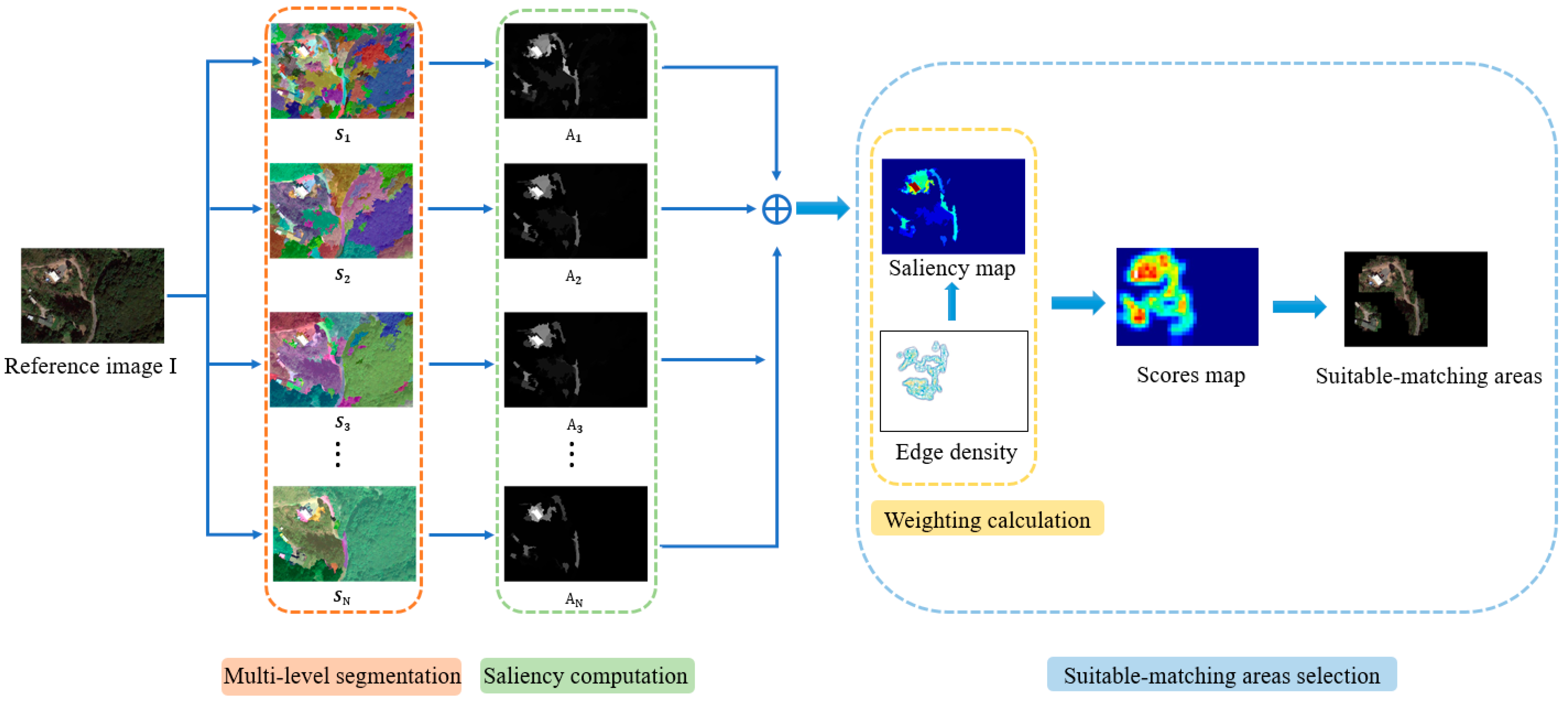
In using template matching technology for target positioning, it is necessary to calculate the similarity between the preprocessed benchmark image and the real-time image. The reference image quality has an essential impact on the matching results and is directly related to the reliability of aircraft navigation and positioning. The suitable-matching areas’ selection approach in this paper consists of three main steps. Figure 1 is the framework of our algorithm.
- Multi-level image segmentation: Divide a reference image into multiple regions according to different segmentation levels, from fine segmentation to coarse segmentation;
- Saliency computation: Extract features for each segmented sub-region, use random forest regression to calculate saliency, and finally, fuse the saliency scores of different segmentation levels to generate a scene saliency map;
- Scene-matching performance analysis and suitable-matching areas’ selection: The saliency score in the sub-region is weighted with the edge density in the area to obtain the adaptability performance score, and the area with a higher score is selected as the benchmark image that participates in the matching verification.
3.1. Multi-Level Segmentation
We first perform multi-level segmentation on the reference image before feature extraction. One image can be decomposed into multiple regions via image segmentation algorithms, and the number of divided regions is controllable. Therefore, we can obtain multi-level image segmentation results S with different degrees of sparsity. Table 1 shows the definition or explanation of the mathematical notations that describe the working principle in this paper.
Given a reference image I, we represent it by a set of N-level segmentation S , where represents the mth layer segmentation result and consists of regions. The larger means that is divided into more regions, which indicates the segmentation result is finer. On the contrary, the smaller means that is divided into fewer regions, which suggests the segmentation result is coarser.
This paper applies the graph-based image segmentation method [30]. Taking the mth layer segmentation result in as an example, it is divided into regions. Each region R can be regarded as a weighted undirected graph , which connects adjacent space areas. V and E express the graph’s vertex and edge sets, respectively. In an image, a single pixel can be seen as a vertex v, and the edge connecting a pair of vertices has a weight , which represents the dissimilarity between pixels:
where represents the gray value of the pixel point . Each channel can be segmented first and then merged if is an RGB image with three channels. In order to reduce the amount of calculation, in constructing graph G, calculations will not be performed on all pairs of pixels. Instead, the grid–graph method is used to calculate the approximate dissimilarity in eight directions around each pixel.
Initially, we treat each pixel as an independent region R, and the essence of segmentation is the process of merging them from large to small according to the similarity between regions. There are two key definitions here [30]. The first is the internal difference of a region, which represents the maximum difference that can be tolerated in the region, that is, the edge with the most remarkable dissimilarity in a region:
The second is the difference between the two regions, which represents the dissimilarity at the most similar point between the two regions, that is, the edge with the smallest dissimilarity among all the edges connecting two regions:
Through Formulas (1) and (2), it can be easily judged whether two regions meet the conditions for merging; that is, when both regions can tolerate their differences, they can be merged into one:
Comparing Diff and Int can determine whether there is a segmentation boundary between the two regions. From this, the judgment function of the segmentation algorithm can be defined as :
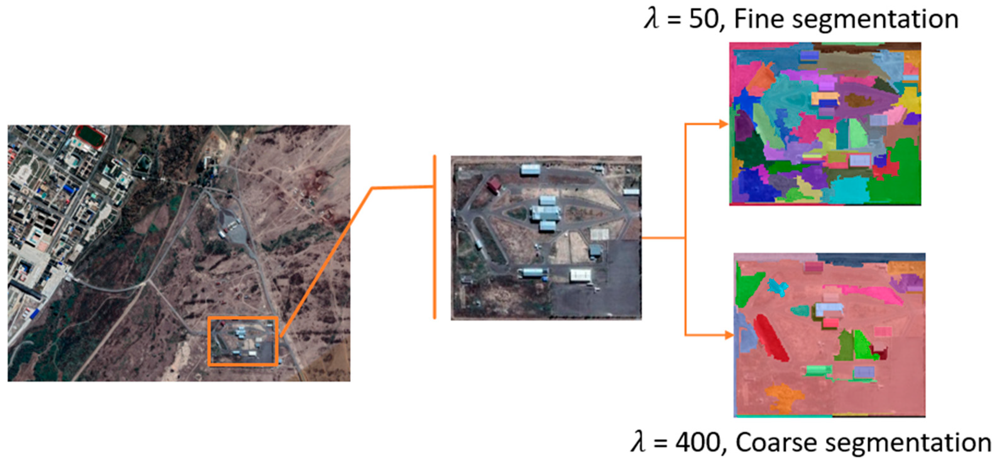
In principle, each isolated pixel can be regarded as a region. However, in this case, only adjacent identical pixels can be merged, inevitably leading to over-segmentation. Therefore, as shown in Formula (6), we give each region a tolerance value , where is the number of pixels in the region. The function of is to control the size of the segmented region. When , each different pixel is an independent region. As increases, the segmented region obtained will also increase, and the entire image belongs to one segmented region if . Therefore, as shown in Figure 2, we can obtain different-level results with different segmentation densities by setting .
Hierarchical screening methods usually require meshing the image first and then using various feature indicators (such as edge density, information entropy, and autocorrelation coefficient) as decision-making attributes to filter the image blocks in sequence to obtain the final suitable-matching area. However, this kind of violent selection will cause the relationship between adjacent image blocks to be ignored, which can easily lead to the omission of suitable-matching areas. By comparing fine segmentation and coarse segmentation (as shown in Figure 2), it can be found that the two contain intersection regions, and some regions in the fine segmentation will form sub-regions in the coarse segmentation result. Therefore, neighborhood information will be forcibly adopted in the subsequent multi-level regional feature fusion, enhancing the correlation and spatial consistency between regions.
3.2. Saliency Computation
In the previous subsection, we decomposed the reference image into different regions. In this section, we will apply three different types of feature descriptors to calculate the saliency score of each region.
First, we utilize the general properties of image regions, including geometric features that describe the size and location of the region and appearance features that characterize the color and texture distribution of the region. Different from regions containing salient objects, backgrounds usually have uniform color distribution and similar texture distribution. Therefore, we extract the above features for each region and obtain the regional property descriptor.
Second, a region can be considered salient to an observer if it differs significantly from its surrounding regions. This paper uses regional contrast descriptors to calculate differences in color and texture features between regions. Taking the segmentation result in as an example, R is a region in , and N is the nearest neighbor region of R. The feature vectors and are respectively defined as the color and texture features of the region R. Similarly, , is the color and texture features of the nearest neighbor region N. The regional contrast descriptor can be obtained by calculating the feature difference:
Specifically, we calculate the absolute element differences (Manhattan Distance) of the color feature vectors, while for texture features, we calculate the distribution divergence (Chi-square Measure) of the texton histogram [31].
There may be misjudgment if we only use the general properties of the image to judge whether a region is salient. We also need to distinguish between the foreground and background of the image. Regions with a similar appearance are likely to come from the background, but the determination of the background depends on the entire image context. When manually marking the suitable-matching areas, the boundary region is generally avoided. That is because the scene information in the boundary region is incomplete and inconvenient for subsequent matching and positioning work. So, when processing the border part, we consider it less salient and classify it as the background. This paper constructs a pseudo-background region B by intercepting the image’s narrow-band boundary of five pixels. We can obtain the regional background descriptor by calculating the color and texture feature difference and use this to determine the background degree of region [32].
We use the random forest regressor pre-trained in the MSRA-B dataset [33]. This dataset has 5000 images in different categories, including indoor, outdoor, animals, natural scenes, etc. It combines the objects marked by nine users that they think are most salient and segments the outlines of salient objects. In training the random forest regressor, we consider a region to be confident if 80% of the pixels belong to the background or the salient object and set its saliency score as 0 or 1. In addition, our experiments used 200 trees during the training to balance the effectiveness and efficiency.
We use the random forest regressor to integrate regional features, including regional property, region contrast, and regional backgroundness for each region in the segmentation map . The features vector sets as the input into the regressor to predict the saliency score of the region. Considering that we perform multi-level image segmentation on the reference image I before feature extraction to obtain S , the multi-level saliency mapping set can be obtained through regressor . Finally, we use least squares estimation to assign different weights w to the set , and the final saliency map is obtained via a linear fusion function:
where N is the number of segmentation levels. Theoretically, the larger the segmentation level N, the more thoroughly we can extract the saliency information of the image. However, larger segmentation levels introduce more computational burden. From an experimental point of view, when N > 5, the incremental effect of saliency extraction slows down, but the time consumption increases rapidly. Therefore, to balance the efficiency and the effectiveness, we set segmentation levels N = 5 in our experiments.
3.3. Matching Performance Measure
We can effectively capture information-rich, distinctive, and non-repetitive areas in the image via multi-level saliency computation. Such areas generally have good matching performance required for benchmark map preparation for scene-matching experiments. However, the saliency map cannot guide the selection directly because the reference image may contain larger or smaller saliency targets, and the selection of suitable-matching areas generally has specific size requirements. Therefore, we need to use edge density to weigh each search window to avoid insignificant parts and ensure the effectiveness of suitable-matching areas’ selection. Calculate the matching performance score for each region:
where is a search window (set a sliding window with a step size of 15) in the saliency map. is the edge density within the window calculated based on the Sobel operator. We will show the difference caused by whether to add edge density to the selection of the suitable-matching areas in the experimental part. We will also show that the higher the matching performance score , the better it can meet the requirements as a suitable-matching area. Algorithm 1 shows the overall process of our approach.
| Algorithm 1: Multi-level Saliency Suitable-matching Area Selection |
| Input: Reference image I Output: Position coordinates of suitable-matching areas |
|
4. Experimental Results
4.1. Dataset and Simulation Real-Time Image Preparation
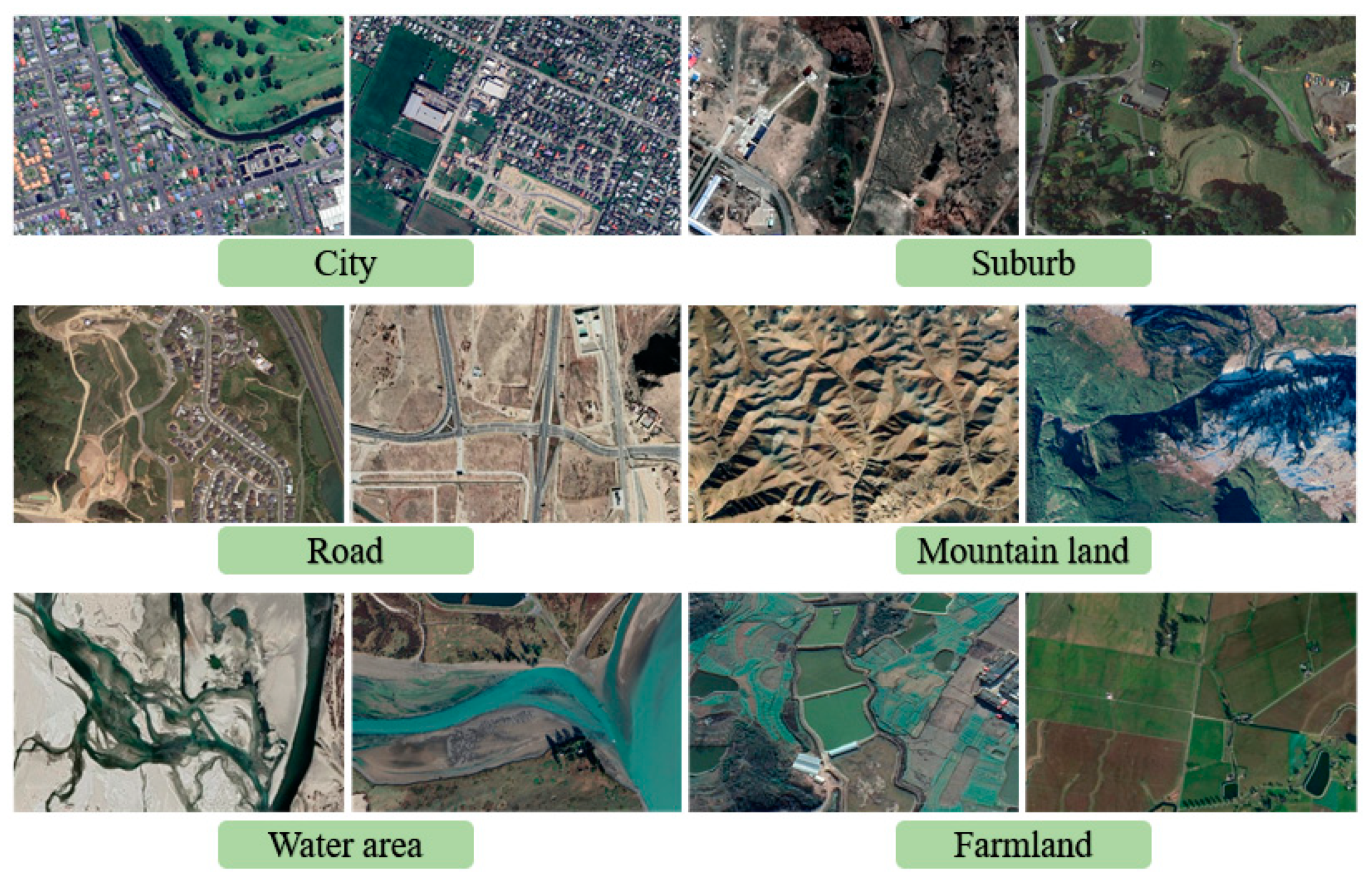
Currently, there is no public standard dataset for scene-matching area selection, and we build a reference image sample set by ourselves. The image dataset contains 500 satellite images of 400 × 600 pixels (as shown in Figure 3). It covers various land features such as cities, suburbs, waters, farmland, roads, and bare land.
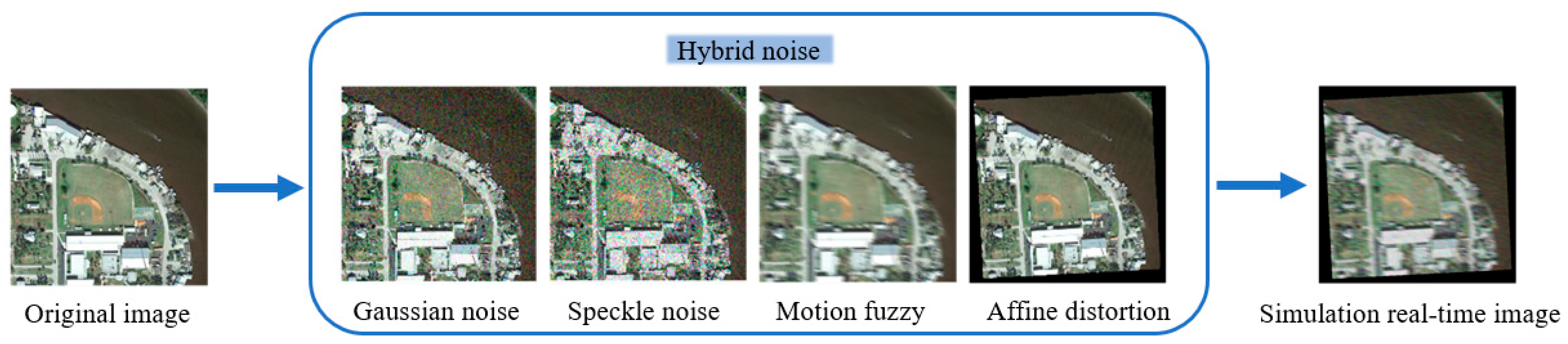
We generate the real-time simulation images by adding noise, blur, and deformation (as shown in Figure 4). This can effectively simulate complex situations such as scale changes, blur, deformation, and low resolution under the actual navigation conditions. Although there are some differences between the simulated real-time image and the actual captured image, the simulation data is easy to generate. In addition, we can know the precise position of the real-time image in the reference image, which facilitates the subsequent accurate calculation of the matching probability and better reflects the appropriate performance.
4.2. Evaluation Indicator
The ‘suitable-matching areas’ selection evaluation indicators are usually related to the matching algorithm. Depending on the task, the matching algorithm is diverse, making the use of unified standards for measurement analysis impossible. However, no matter what matching method is used, the matching performance of the selected areas can be evaluated through matching error and matching probability.
The matching error refers to the degree of similarity between the matching and actual positions. We measure the matching error between the simulation real-time image and the reference image by calculating the overlap rate :
where represents the number of pixels in an area, represents the matching result, and represents the actual position. The larger the value, the smaller the matching error and the better the matching performance. The match is considered successful if is within the allowed error range. When the matching algorithm is fixed, record whether each candidate area can be matched successfully. We can obtain the matching probability P = n/N, where n is the number of areas that can be successfully matched and N is the number of candidate areas in an image. The matching reliability of the selected areas can be measured by calculating the ratio of the two.
In our experimental design, we will use matching error and matching probability evaluation indicators to conduct a quantitative analysis of our method. Among them, we will determine a successful match when the overlap rate is greater than 0.9 and calculate the matching probability based on this.
4.3. Adaptability Analysis and Suitable-Matching Areas’ Selection
In order to verify the effectiveness of our approach, which we call multi-level saliency suitable-matching areas’ selection (MSAS), we conduct a comparative analysis with the representative hierarchical screening (HS) method. We select the same feature indicators as [2] for HS: image variance (), edge density (), information entropy (), and primary and secondary peak ratio ( > 1.2) via the multi-attribute decision-making method, to filter out the suitable-matching areas in a given reference image.
To verify the matching performance, we select the most commonly used normalized cross-correlation (NCC) in navigation as the matching algorithm. It can cope with illumination changes and noise effects well and finds the target position quickly and efficiently. In order to verify that the higher the score , the better it can meet the selection requirements of the suitable-matching area, we screened the top 15% and the top 10% of the image areas with scores as candidate matching areas to compare with the HS method.
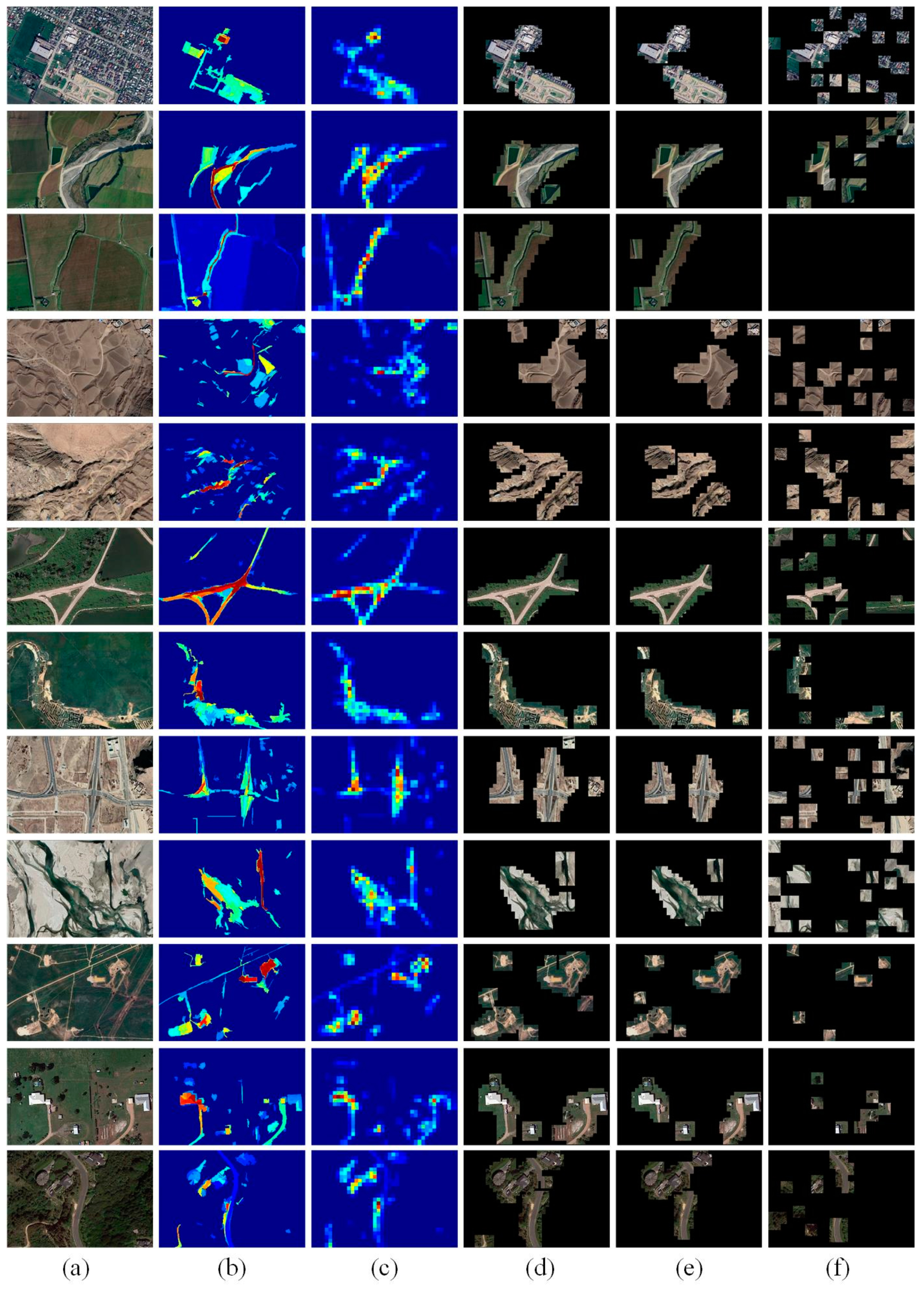
We illustrate the advantages of our approach via qualitative analysis and quantitative analysis. Figure 5 shows the candidate areas selected by the MSAS and HS for matching template preparation. The second column in Figure 5 shows the salient feature map extracted from the reference image. The third column is the matching performance score map obtained after weighted calculation, allowing us to intuitively see each position’s matching ability. The next three columns are the areas corresponding to the top 15% and the top 10% of MSAS algorithm scores and the HS method recommendation results. It can be found that there are many mis-selections and omissions in the HS method. In contrast, our method can combine the overall information of the image for screening. The image information contained in our candidate areas is rich and significant, which can well meet the selection requirements.
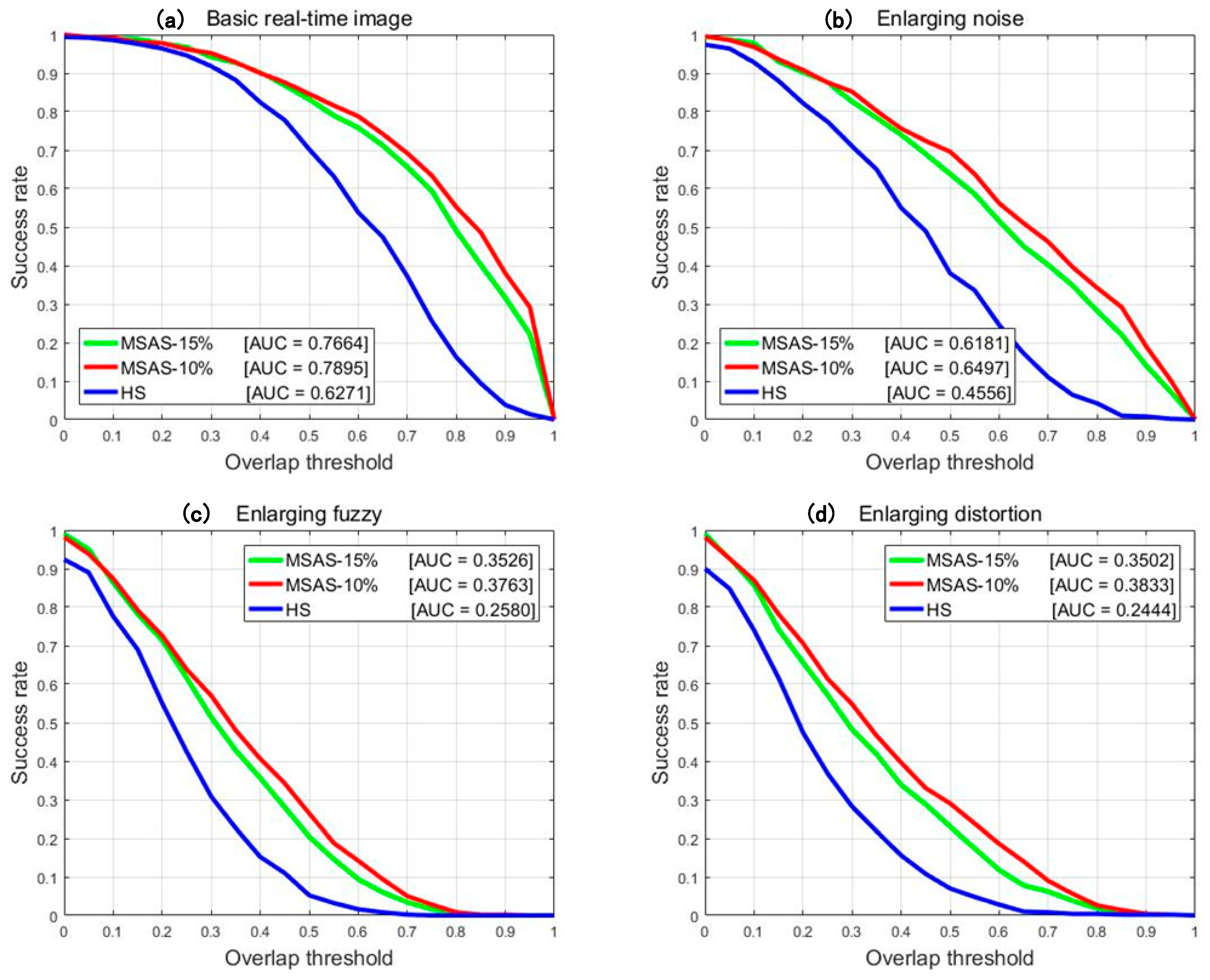
We use NCC to match the simulated real-time image of each candidate area with the reference image and count the matching errors. Then, calculate the matching probability of each image in the dataset. We draw the receiver operating characteristic curve (ROC) (as shown in Figure 6) and calculate the Area-under-curve (AUC) value of each curve (as shown in Table 2) to quantify the overall accuracy, reflecting the selected area’s overall matching performance.
With essential noise, blur, and deformation added, the overall matching accuracy of the top 10% areas of the MSAS matching performance score can reach 0.7895, which is 25.9% higher than HS. The top 15% of areas’ matching accuracy reaches 0.7664, which is 22.2% higher than HS. It can be observed from the ROC curve in Figure 6 that the matching accuracy of our method decreases more slowly when the noise, blur, and deformation are increased, respectively. Combining the data in Table 2, we can see that MSAS has noticeable performance improvements under various complex interferences. In summary, our approach has more comprehensive advantages in analyzing the regional matching performance.
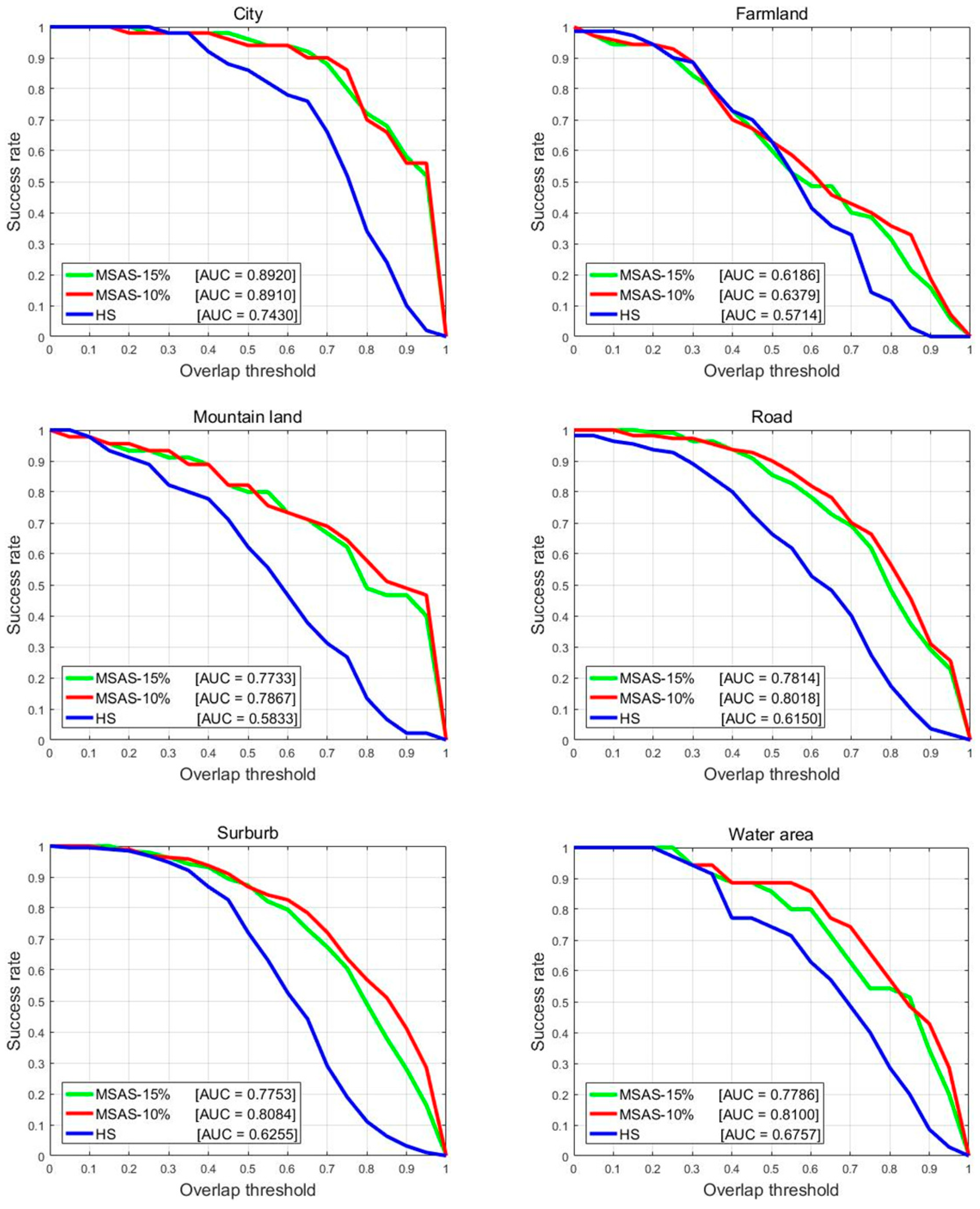
Due to different scene categories, the color and texture information contained in the images vary greatly. Therefore, it is necessary to analyze the matching performance of the selected area according to different scene categories. Table 3 shows the number of images for each image category in our dataset and the corresponding AUC scores from MSAS and HS. It can be seen that our approach has better matching accuracy in the selected areas in six different scenarios. Combined with the ROC curve in Figure 7, we can clearly see the performance difference between MSAS and HS in terms of matching performance analysis, which confirms the effectiveness and generalization of our approach from the side.
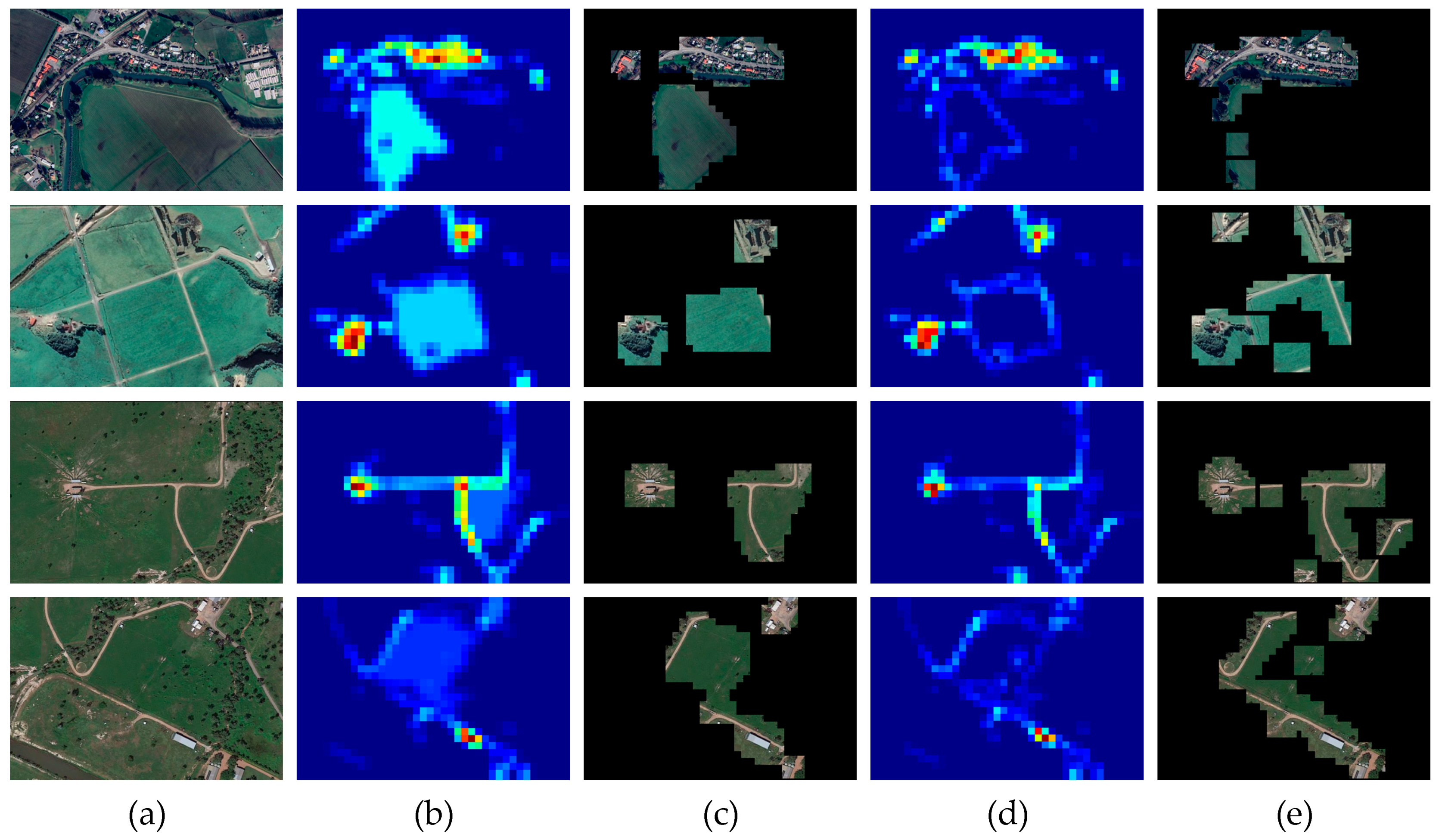
In Section 3.3, we mentioned that there are size requirements for the production of template images. In order to screen the suitable-matching area more reasonably and effectively, when we construct the score map, we give the search window a certain weight based on the regional edge density. In Figure 8, columns (b) and (c) show the results of directly selecting high-salience response areas without weighting, and columns (d) and (e) show the results of candidate areas after adding weights. Through comparison, the weighted calculation can effectively filter out the parts that are not rich in information, and thus, make more reliable use of the salient features of the image. At the same time, the boundary processing of candidate areas is also more delicate.
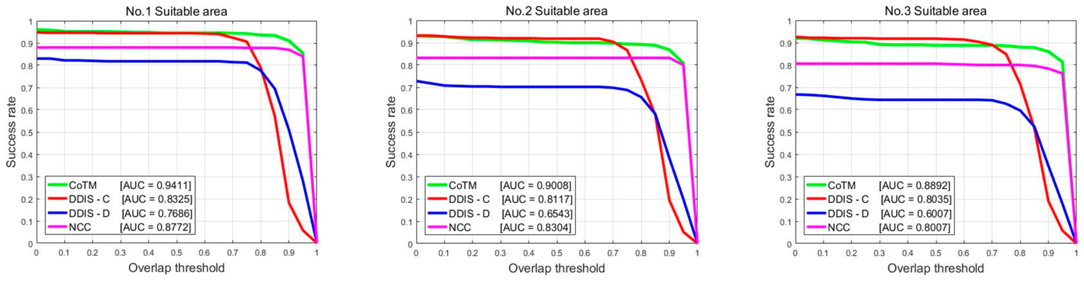
Theoretically, the matching probability of a scene area is not only related to the image content but also to the matching algorithm. The matching errors calculated by different matching algorithms may differ for the same area. However, we can obtain good matching results for areas with good matching performance no matter what matching algorithm we use. In addition to the NCC used above, we also use the DDIS [34] (based on color feature DDIS-C and depth feature DDIS-D) and the CoTM [35] matching algorithm, which currently has the best matching results in complex scenes. For the 500 reference images in the dataset, we select three areas with a size of in each image as suitable-matching areas. The area with the highest matching performance score is the No.1 suitable-matching area. In order to ensure that the three selected areas do not overlap, the score of the No.1 area is cleared to zero after finding the maximum value area. Repeating the above operations, we can find the No.2 and No.3 suitable-matching areas.
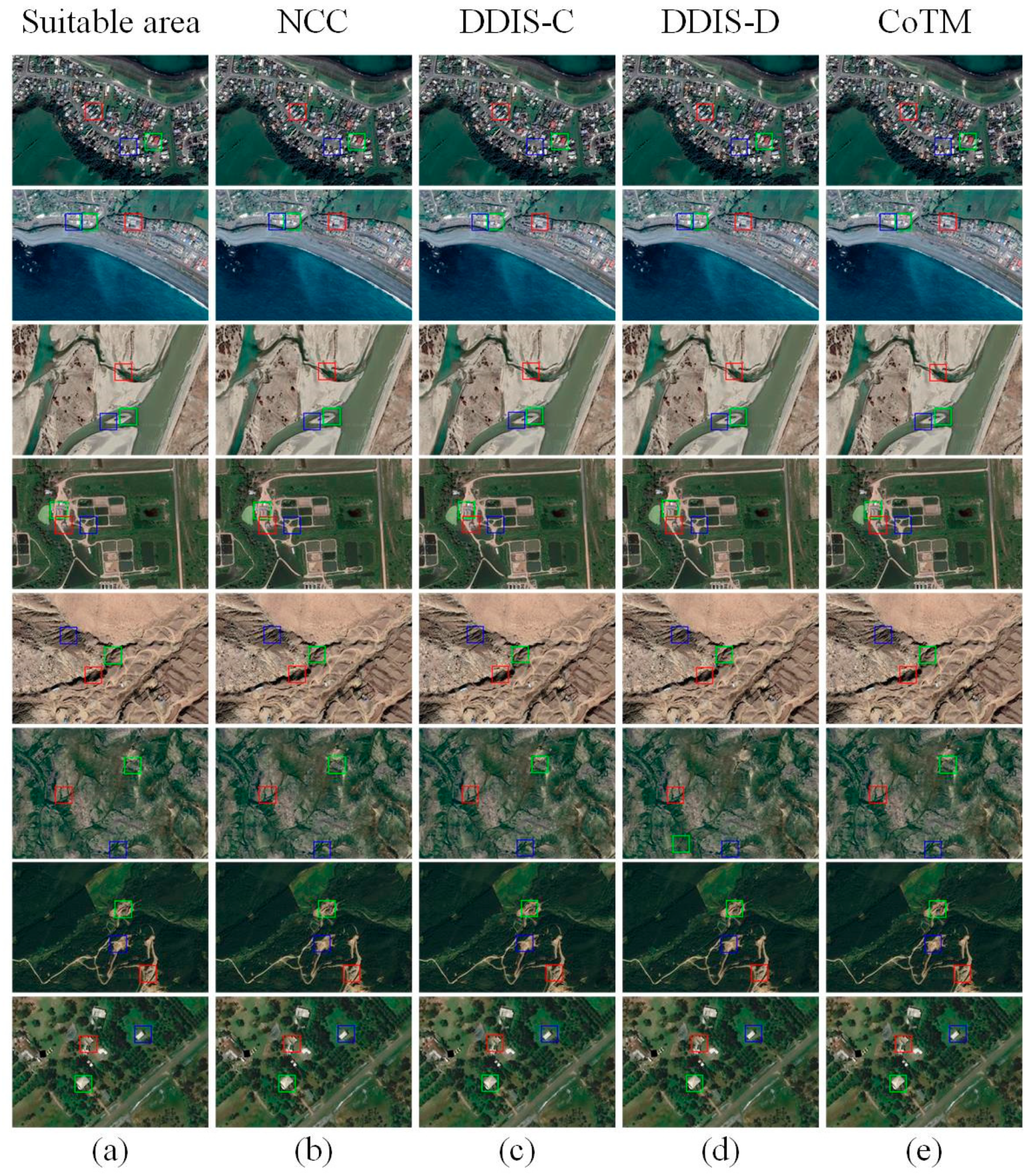
Next, we use various matching algorithms to match and position the simulated real-time images of the selected areas in the reference images and conduct quantitative and qualitative analysis of the matching results. Figure 9 plots the ROC curve, and Table 4 shows the AUC value corresponding to each curve. It can be seen that the No.1 areas have the highest matching accuracy. The other two areas also have high matching performance. Figure 10 shows the results of some matching experiments. The first column is the three suitable-matching areas selected by our approach for each image. The remaining four columns show the positioning results of different matching algorithms based on the simulated real-time image. It can be found that for each selected suitable-matching area, different matching algorithms can basically match the target location.
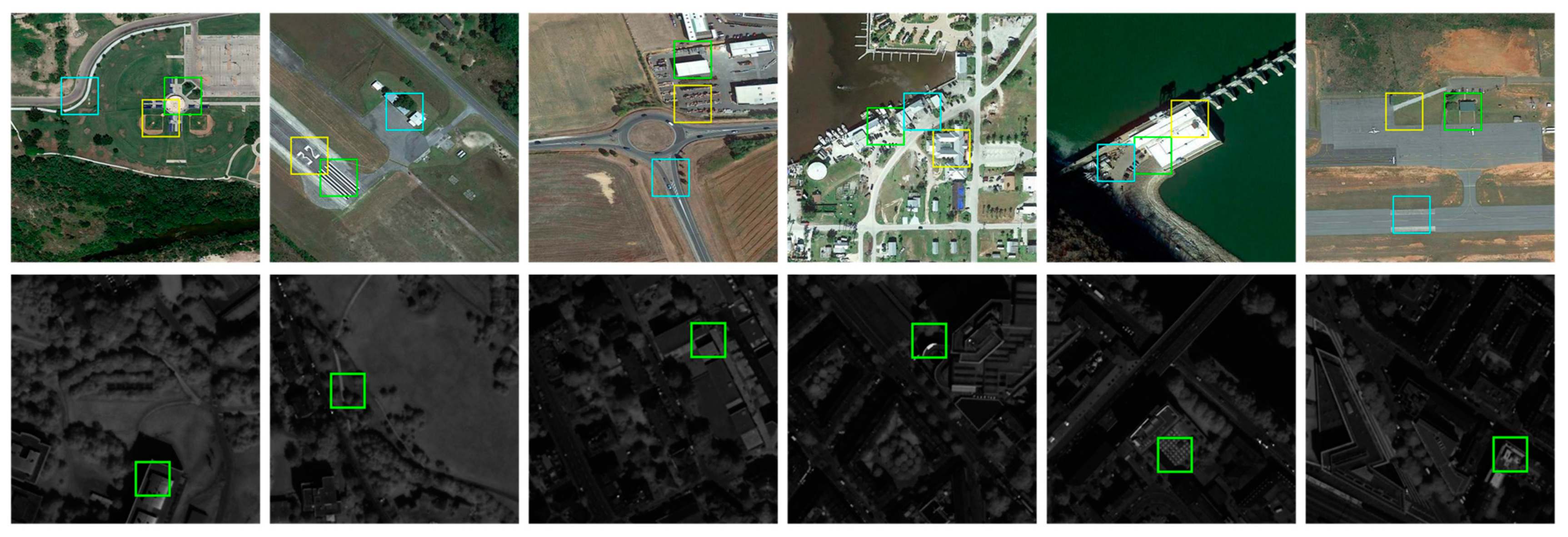
In order to verify the suitable-matching areas’ selection effect in this paper under different imaging mechanisms, we conducted experiments on aerial and near-infrared images, respectively. In Figure 11, the first row selects three 50 × 50 pixels suitable-matching areas from the 512 × 512 size aerial images, and the second row selects one 40 × 40 pixel from the 300 × 300 size near-infrared images. It can be seen that our algorithm selects scene areas with clear outlines, rich textures, and noticeable features as suitable-matching areas, which reflects that our approach can be applied under different imaging mechanisms and has good versatility.
5. Conclusions
In this paper, we propose the suitable-matching areas’ selection method based on multi-level saliency to address the problem of reference map preparation in scene-matching navigation. We perform multi-level segmentation before feature extraction to enhance adjacent regions’ spatial consistency. We fuse three feature descriptors to strengthen the connection between different characteristics. It improves the one-sidedness of the traditional hierarchical rule method in scene description and the low versatility caused by the fixed filtering threshold. To utilize the salient areas more effectively and reduce omission and wrong selection, we perform edge-density weighted calculations on the saliency map to obtain the matching performance score. Compared with the traditional hierarchical screening methods, our approach’s matching performance evaluation capability improves by at least 22.2%. By verifying multiple matching algorithms on the top suitable-matching area we selected, the average matching success rate can reach 0.8549. The results show that our method can effectively identify areas with high matching performance in the image and we can achieve good results when facing different scene categories. In addition, our approach is more than just targeting a specific image. Our method can be more widely used in suitable-matching area selection applications for scene-matching navigation with different imaging mechanisms, such as aerial, satellite, and near-infrared images. In the future, we can adjust the salient feature extraction algorithm according to the image characteristics of different imaging mechanisms to make the suitable-matching area selection method more targeted and professional. We will conduct more in-depth research on the applicable scope of image scenes.
Author Contributions
Conceptualization, S.J., H.L. and Y.L.; Data curation, S.J.; Methodology, S.J.; Software, S.J.; Validation, S.J.; Visualization, S.J.; Writing—original draft, S.J.; Writing—review and editing, S.J., H.L. and Y.L. All authors have read and agreed to the published version of the manuscript.
Funding
This research was funded by Infrared vision theory and method, grant number E31A040301 and the APC was funded by Infrared vision theory and method.
Data Availability Statement
Data sharing is not applicable to this article.
Conflicts of Interest
The authors declare no conflicts of interest.
References
- Diwani, D.; Chougule, A.; Mukhopadhyay, D. Artificial intelligence based missile guidance system. In Proceedings of the 2020 7th International Conference on Signal Processing and Integrated Networks (SPIN), Noida, India, 27–28 February 2020; pp. 873–878. [Google Scholar]
- Fan, J.W.; Yang, X.G.; Lu, R.T.; Li, Q.G.; Xia, H. Intelligent scene matching suitable area selection method based on remote sensing image. J. Chin. Inert. Technol. 2023, 31, 14–23. [Google Scholar]
- Raković, D.M.; Simonović, A.; Grbović, A.M. UAV Positioning and Navigation-Review. In Experimental and Computational Investigations in Engineering, Proceedings of the International Conference of Experimental and Numerical Investigations and New Technologies, CNNTech 2020, Zlatibor Mountain, Serbia, 30 June–3 July 2020; Springer: Cham, Switzerland, 2020; pp. 220–256. [Google Scholar]
- Dou, Q.F.; Du, T.; Qiu, Z.B.; Wang, S.P.; Yang, J. An adaptive anti-disturbance navigation method for polarized skylight-based autonomous integrated navigation system. Measurement 2022, 202, 111847. [Google Scholar] [CrossRef]
- Gyagenda, N.; Hatilima, J.V.; Roth, H.; Zhmud, V. A review of GNSS-independent UAV navigation techniques. Robot. Auton. Syst. 2022, 152, 104069. [Google Scholar] [CrossRef]
- Boiteau, S.; Vanegas, F.; Sandino, J.; Gonzalez, F.; Galvez-Serna, J. Autonomous UAV Navigation for Target Detection in Visually Degraded and GPS Denied Environments. In Proceedings of the 2023 IEEE Aerospace Conference, Big Sky, MT, USA, 4–11 March 2023; pp. 1–10. [Google Scholar]
- Li, X.; Zhang, G.; Cui, H.; Ma, J.; Wang, W. Analysis of the Matchability of Reference Imagery for Aircraft Based on Regional Scene Perception. Remote Sens. 2023, 15, 4353. [Google Scholar] [CrossRef]
- Shahoud, A.; Shashev, D.; Shidlovskiy, S. Design of a navigation system based on scene matching and software in the loop simulation. In Proceedings of the 2021 International Conference on Information Technology (ICIT), Amman, Jordan, 14–15 July 2021; pp. 412–417. [Google Scholar]
- Jin, Z.L.; Wang, X.Z.; Moran, B.; Pan, Q.; Zhao, C.H. Multi-region scene matching based localisation for autonomous vision navigation of UAVs. J. Navig. 2016, 69, 1215–1233. [Google Scholar] [CrossRef]
- Zhang, S.; Duan, X.; Peng, L. Uncertainty quantification towards filtering optimization in scene matching aided navigation systems. Int. J. Uncertain. Quantif. 2016, 6, 127–140. [Google Scholar] [CrossRef]
- Leng, X.F. Research on the Key Technology for Scene Matching Aided Navigation System Based on Image Features. Ph.D. Thesis, Nanjing University of Aeronautics and Astronautics, Nanjing, China, 2007. [Google Scholar]
- Wang, J.Z. Research on Key Technologies of Scene Matching Areas Selection of Cruise Missile. Master’s Thesis, National University of Defense Technology, Changsha, China, 2015. [Google Scholar]
- Chen, R.; Zhang, Q.Q.; Zhao, L. Optimal selection and adaptability analysis of matching area for terrain aided navigation. IET Radar Sonar Navig. 2021, 15, 1702–1714. [Google Scholar] [CrossRef]
- Cao, F.; Yang, X.G.; Miao, D.; Zhang, Y.P. Study on reference image selection roles for scene matching guidance. Appl. Res. Comput. 2005, 5, 137–139. [Google Scholar]
- Pang, S.N.; Kim, H.C.; Kim, D.; Bang, S.Y. Prediction of the suitability for image-matching based on self-similarity of vision contents. Image Vis. Comput. 2004, 22, 355–365. [Google Scholar] [CrossRef]
- Yang, X.; Cao, F.; Huang, X. Reference image preparation approach for scene matching simulation. J. Syst. Simul. 2010, 4, 850–852. [Google Scholar]
- Hua, H.Y.; Shi, Z.L.; Liu, Y.P. A metric based on saliency line feature extraction and connection for matching area selection. In Proceedings of the Second Target Recognition and Artificial Intelligence Summit Forum, Shenyang, China, 28–30 August 2020; pp. 140–145. [Google Scholar]
- Shahoud, A.; Shashev, D.; Shidlovskiy, S. Detection of good matching areas using convolutional neural networks in scene matching-based navigation systems. In Proceedings of the 31st International Conference on Computer Graphics and Vision, Nizhny Novgorod, Russia, 27–30 September 2021; pp. 27–30. [Google Scholar]
- Borji, A.; Cheng, M.M.; Hou, Q.; Jiang, H.; Li, J. Salient object detection: A survey. Comput. Vis. Media 2019, 5, 117–150. [Google Scholar] [CrossRef]
- Gupta, A.K.; Seal, A.; Prasad, M.; Khanna, P. Salient object detection techniques in computer vision—A survey. Entropy 2020, 22, 1174. [Google Scholar] [CrossRef] [PubMed]
- Johnson, M. Analytical development and test results of acquisition probability for terrain correlation devices used in navigation systems. In Proceedings of the AIAA 10th Aerospace Sciences Meeting, San Diego, CA, USA, 17–19 January 1972; p. 122. [Google Scholar]
- Luo, H.B.; Chang, Z.; Yu, X.R.; Ding, Q.H. Automatic suitable-matching area selection method based on multi-feature fusion. Infrared Laser Eng. 2011, 40, 2037–2041. [Google Scholar]
- Zhang, X.C.; He, Z.W.; Liang, Y.H.; Zeng, P. Selection method for scene matching area based on information entropy. In Proceedings of the 2012 Fifth International Symposium on Computational Intelligence and Design (ISCID), Hangzhou, China, 28–29 October 2012; Volume 1, pp. 364–368. [Google Scholar]
- Qu, S.J.; Tao, L.; Zheng, T.Y. A novel matching suitability analysis method based on fusion of multi-indexes. Radar Sci. Technol. 2015, 13, 415–420. [Google Scholar]
- Zhang, Y.Y.; Su, J.; Li, B. SAR scene matching area selection based on multi-attribute comprehensive analysis. J. Proj. Rocket. Missile Guid. 2016, 36, 104–108. [Google Scholar]
- Yang, Z.H.; Chen, Y.; Qian, X.Q.; Yuan, M.; Gao, E.T. Predicting the suitability for scene matching using SVM. In Proceedings of the 2008 International Conference on Audio, Language and Image Processing, Shanghai, China, 7–9 July 2008; pp. 743–747. [Google Scholar]
- Sharif, U.; Mehmood, Z.; Mahmood, T.; Javid, M.A.; Rehman, A.; Saba, T. Scene analysis and search using local features and support vector machine for effective content-based image retrieval. Artif. Intell. Rev. 2019, 52, 901–925. [Google Scholar] [CrossRef]
- Yang, J. Suitable Matching Area Selection Method Based on Deep Learning. Master’s Thesis, Huazhong University of Science and Technology, Wuhan, China, 2019. [Google Scholar]
- Sheng, H.K. Research on Matching Area Selection of SAR Image Based on SA-HRNet. Master’s Thesis, Huazhong University of Science and Technology, Wuhan, China, 2020. [Google Scholar]
- Felzenszwalb, P.F.; Huttenlocher, D.P. Efficient graph-based image segmentation. Int. J. Comput. Vis. 2004, 59, 167–181. [Google Scholar] [CrossRef]
- Khaldi, B.; Aiadi, O.; Lamine, K.M. Image representation using complete multi-texton histogram. Multimed. Tools Appl. 2020, 79, 8267–8285. [Google Scholar] [CrossRef]
- Jiang, H.; Wang, J.; Yuan, Z.; Wu, Y.; Zheng, N.; Li, S. Salient object detection: A discriminative regional feature integration approach. In Proceedings of the IEEE/CVF Conference on Computer Vision and Pattern Recognition (CVPR), Portland, OR, USA, 23–27 June 2013; pp. 2083–2090. [Google Scholar]
- Liu, T.; Yuan, Z.J.; Sun, J.; Wang, J.D.; Zheng, N.N.; Tang, X.O.; Shum, H.Y. Learning to detect a salient object. IEEE Trans. Pattern Anal. Mach. Intell. 2010, 33, 353–367. [Google Scholar]
- Talmi, I.; Mechrez, R.; Zelnik-Manor, L. Template matching with deformable diversity similarity. In Proceedings of the IEEE/CVF Conference on Computer Vision and Pattern Recognition (CVPR), Honolulu, HI, USA, 21–26 July 2017; pp. 175–183. [Google Scholar]
- Kat, R.; Jevnisek, R.; Avidan, S. Matching pixels using co-occurrence statistics. In Proceedings of the IEEE/CVF Conference on Computer Vision and Pattern Recognition (CVPR), Salt Lake City, UT, USA, 18–22 June 2018; pp. 1751–1759. [Google Scholar]
Figure 1.
The framework of our proposed multi-level saliency suitable-matching areas’ selection (MSAS) approach.
Figure 1.
The framework of our proposed multi-level saliency suitable-matching areas’ selection (MSAS) approach.

Figure 2.
Different levels of segmentation results: When , the image is divided into many regions, forming fine segmentation. When , the image is divided into very few regions, forming coarse segmentation.
Figure 2.
Different levels of segmentation results: When , the image is divided into many regions, forming fine segmentation. When , the image is divided into very few regions, forming coarse segmentation.

Figure 3.
Examples of the main scene types in our dataset.

Figure 4.
The preparation process of simulation real-time image.

Figure 5.
The candidate areas for matching template preparation: (a) reference image; (b) saliency map; (c) matching performance scores map; (d) MSAS—15%; (e) MSAS—10%; and (f) HS.
Figure 5.
The candidate areas for matching template preparation: (a) reference image; (b) saliency map; (c) matching performance scores map; (d) MSAS—15%; (e) MSAS—10%; and (f) HS.

Figure 6.
Accuracy: Success curves showing the fraction of examples of matching probability > . (a) Use the basic simulation real-time images; (b) increase the noise impact of simulation real-time images; (c) increase the blurring effect of simulation real-time images; and (d) increase the deformation effect of simulation real-time images.

Figure 7.
Accuracy: Six different scene categories (including city, farmland, mountain land, road, suburb, and water area).
Figure 7.
Accuracy: Six different scene categories (including city, farmland, mountain land, road, suburb, and water area).

Figure 8.
Result of edge density weighting: (a) reference image; (b) scores map without weighting; (c) suitable-matching candidate areas’ selection without weighting; (d) scores map with weighting; and (e) suitable-matching candidate areas’ selection with weighting.
Figure 8.
Result of edge density weighting: (a) reference image; (b) scores map without weighting; (c) suitable-matching candidate areas’ selection without weighting; (d) scores map with weighting; and (e) suitable-matching candidate areas’ selection with weighting.

Figure 9.
Matching accuracy using different matching algorithms.

Figure 10.
Matching results of different matching algorithms: (a) suitable area; (b) NCC; (c) DDIS-C; (d) DDIS-D; (e) CoTM. The green box is the No.1 suitable-matching area, the red box is the No.2 suitable-matching area, and the blue box is the No.3 suitable-matching area.
Figure 10.
Matching results of different matching algorithms: (a) suitable area; (b) NCC; (c) DDIS-C; (d) DDIS-D; (e) CoTM. The green box is the No.1 suitable-matching area, the red box is the No.2 suitable-matching area, and the blue box is the No.3 suitable-matching area.

Figure 11.
The results of suitable-matching areas’ selection for aerial image and near-infrared image.
Figure 11.
The results of suitable-matching areas’ selection for aerial image and near-infrared image.


Table 1.
Define or explain the mathematical notations that describe the working principle of the proposed approach.
Table 1.
Define or explain the mathematical notations that describe the working principle of the proposed approach.
| Mathematical Notation | Definition or Explanation |
|---|---|
| a set of N-level segmentation, S , | |
| the number of segmented areas included in the mth layer | |
| the mth layer contain | |
| a weighted undirected graph, | |
| a set of graph’s vertex, | |
| a set of graph’s edge |
Table 2.
AUC score of different simulation real-time images.
| Method | Basic | Noise + | Fuzzy + | Distortion + | ||||
|---|---|---|---|---|---|---|---|---|
| AUC | Increase | AUC | Increase | AUC | Increase | AUC | Increase | |
| MSAS-10% | 0.7895 | 25.9% | 0.6497 | 42.6% | 0.3763 | 45.9% | 0.3833 | 56.8% |
| MSAS-15% | 0.7664 | 22.2% | 0.6181 | 35.7% | 0.3526 | 36.7% | 0.3502 | 43.3% |
| HS | 0.6271 | 0.4556 | 0.2580 | 0.2444 | ||||
Table 3.
AUC score of six different scene categories.
| Method | City | Farmland | Mountain Land | Road | Suburb | Water Area |
|---|---|---|---|---|---|---|
| 50 | 70 | 45 | 110 | 190 | 35 | |
| MSAS-10% | 0.8910 | 0.6379 | 0.7867 | 0.8018 | 0.8084 | 0.8100 |
| MSAS-15% | 0.8920 | 0.6186 | 0.7733 | 0.7814 | 0.7753 | 0.7786 |
| HS | 0.7430 | 0.5714 | 0.5833 | 0.6150 | 0.6255 | 0.6757 |
Table 4.
AUC score of different matching algorithms.
| Suitable-Matching Area | CoTM | DDIS-Color | DDIS-Deep | NCC | Mean |
|---|---|---|---|---|---|
| No.1 | 0.9411 | 0.8325 | 0.7686 | 0.8772 | 0.8549 |
| No.2 | 0.9008 | 0.8117 | 0.6543 | 0.8304 | 0.7993 |
| No.3 | 0.8892 | 0.8305 | 0.6007 | 0.8007 | 0.7803 |
Disclaimer/Publisher’s Note: The statements, opinions and data contained in all publications are solely those of the individual author(s) and contributor(s) and not of MDPI and/or the editor(s). MDPI and/or the editor(s) disclaim responsibility for any injury to people or property resulting from any ideas, methods, instructions or products referred to in the content. |
© 2023 by the authors. Licensee MDPI, Basel, Switzerland. This article is an open access article distributed under the terms and conditions of the Creative Commons Attribution (CC BY) license (https://creativecommons.org/licenses/by/4.0/).
Share and Cite
MDPI and ACS Style
Jiang, S.; Luo, H.; Liu, Y. Suitable-Matching Areas’ Selection Method Based on Multi-Level Saliency. Remote Sens. 2024, 16, 161. https://doi.org/10.3390/rs16010161
AMA Style
Jiang S, Luo H, Liu Y. Suitable-Matching Areas’ Selection Method Based on Multi-Level Saliency. Remote Sensing. 2024; 16(1):161. https://doi.org/10.3390/rs16010161
Chicago/Turabian StyleJiang, Supeng, Haibo Luo, and Yunpeng Liu. 2024. "Suitable-Matching Areas’ Selection Method Based on Multi-Level Saliency" Remote Sensing 16, no. 1: 161. https://doi.org/10.3390/rs16010161
Note that from the first issue of 2016, this journal uses article numbers instead of page numbers. See further details here.