
Sparse Mix-Attention Transformer for Multispectral Image and Hyperspectral Image Fusion

1
Jiangsu Key Laboratory of Big Data Analysis Technology (B-DAT), Jiangsu Collaborative Innovation Center of Atmospheric Environment and Equipment Technology (CICAEET), Nanjing University of Information Science and Technology, Nanjing 210044, China
2
School of Electronic Information Engineering, Suzhou Vocational University, Suzhou 215104, China
*
Author to whom correspondence should be addressed.
Remote Sens. 2024, 16(1), 144; https://doi.org/10.3390/rs16010144
Submission received: 2 November 2023
/
Revised: 25 December 2023
/
Accepted: 27 December 2023
/
Published: 29 December 2023
(This article belongs to the Special Issue Remote Sensing Data Fusion and Applications)
Abstract
:Multispectral image (MSI) and hyperspectral image (HSI) fusion (MHIF) aims to address the challenge of acquiring high-resolution (HR) HSI images. This field combines a low-resolution (LR) HSI with an HR-MSI to reconstruct HR-HSIs. Existing methods directly utilize transformers to perform feature extraction and fusion. Despite the demonstrated success, there exist two limitations: (1) Employing the entire transformer model for feature extraction and fusion fails to fully harness the potential of the transformer in integrating the spectral information of the HSI and spatial information of the MSI. (2) HSIs have a strong spectral correlation and exhibit sparsity in the spatial domain. Existing transformer-based models do not optimize this physical property, which makes their methods prone to spectral distortion. To accomplish these issues, this paper introduces a novel framework for MHIF called a Sparse Mix-Attention Transformer (SMAformer). Specifically, to fully harness the advantages of the transformer architecture, we propose a Spectral Mix-Attention Block (SMAB), which concatenates the keys and values extracted from LR-HSIs and HR-MSIs to create a new multihead attention module. This design facilitates the extraction of detailed long-range information across spatial and spectral dimensions. Additionally, to address the spatial sparsity inherent in HSIs, we incorporated a sparse mechanism within the core of the SMAB called the Sparse Spectral Mix-Attention Block (SSMAB). In the SSMAB, we compute attention maps from queries and keys and select the K highly correlated values as the sparse-attention map. This approach enables us to achieve a sparse representation of spatial information while eliminating spatially disruptive noise. Extensive experiments conducted on three synthetic benchmark datasets, namely CAVE, Harvard, and Pavia Center, demonstrate that the SMAformer method outperforms state-of-the-art methods.
1. Introduction
Multispectral image (MSI) and hyperspectral image (HSI) fusion (MHIF) aims to obtain a high-resolution (HR) HSI by fusing a low-resolution (LR) HSI and an HR-MSI in the same scene. Compared to traditional images containing only a few bands (such as RGB), HSIs offer the advantage of capturing more spectral information about the same scene. Research has demonstrated the significant benefits of HSIs in various vision tasks, including tracking [1], segmentation [2], and classification [3].
Early methods of MHIF drew inspiration from pansharpening techniques used in remote-sensing images. These methods, such as component substitution (CS) [4,5] and multiresolution analysis (MRA) [6,7,8], were computationally efficient. However, they face challenges in terms of the fusion quality and easily lead to spectral distortion. This can be attributed to the fact that a single panchromatic image inherently contains less spectral information compared to HSIs. The subsequent model-based techniques, e.g., Bayesian-based [9,10], tensor-based [11,12], and matrix factorization-based methods [13,14], rely on prior knowledge of HSIs to address this issue. For example, Wei et al. [15] suppose the target image resides in a lower-dimensional subspace. A carefully designed sparse regularization term is incorporated, and a fusion problem is addressed through optimization algorithms. Kawakami et al. [13] assume that each spectrum can be linearly represented by a set of spectral atomic components. Applying the decomposition algorithm to the hyperspectral input enables the estimation of the basis representing the reflection spectra, which is subsequently integrated with the MSI image to yield the final result. However, it is important to note that these prior knowledge sources are artificially designed and may not encompass all the characteristics of real data. As a result, the ability of the model to generalize is significantly constrained.
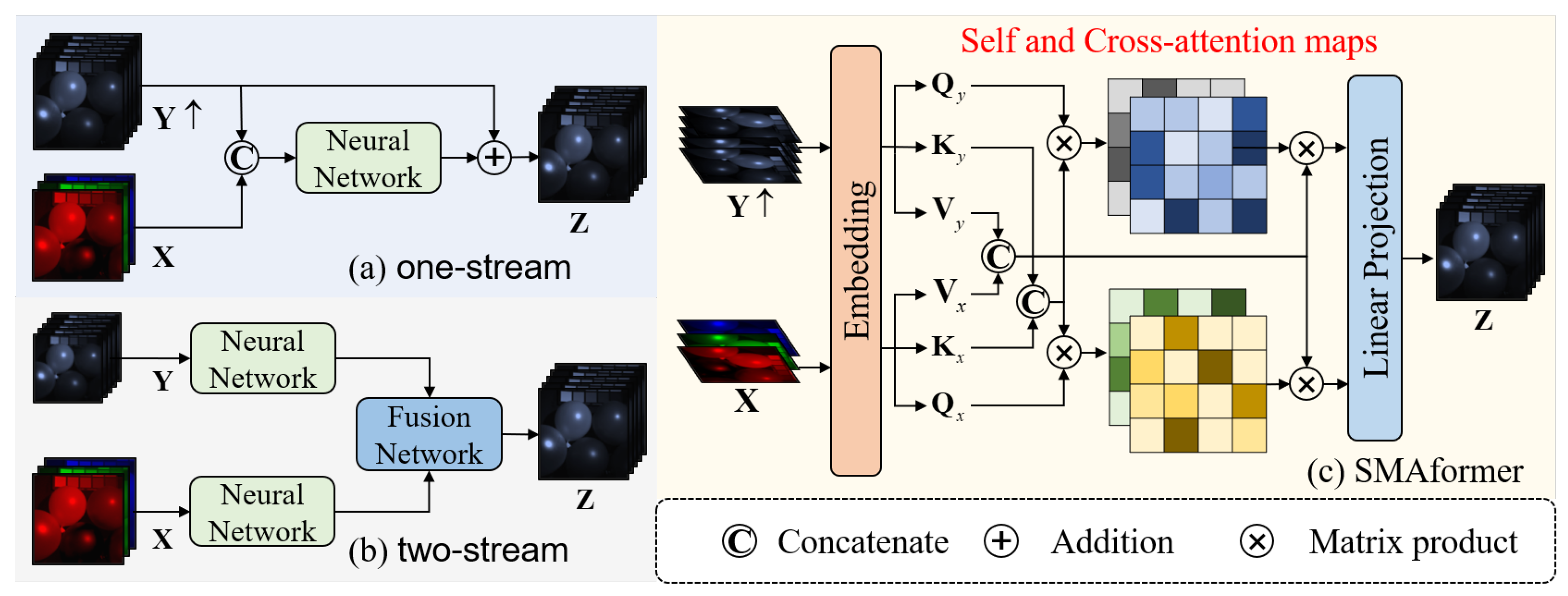
In recent years, deep learning methods have shown remarkable advancements in various domains of computer vision, including super-resolution (SR) tasks [16,17]. The field of MHIF has also witnessed significant exploration in applying deep learning methods. One of the earliest deep learning approaches in this field is based on a 3D convolutional neural network (CNN) [18], which has achieved impressive results. Xie et al. [19] have successfully combined deep learning algorithms with optimization algorithms to enhance interpretability. These methods can be broadly categorized into two types, as shown in Figure 1. The first type (see Figure 1a) directly concatenates the upsampled HSI and MSI as the input and passes them through a neural network to obtain the reconstructed image [20,21]. The second type (see Figure 1b) employs two independent neural networks to extract features from HSIs and MSIs separately, and a fusion module is then utilized to generate the final output [22,23]. Although these methods have shown advancements compared to traditional approaches, they still exhibit certain limitations. The restricted receptive field of CNNs hinders the effective capture of global information, resulting in constraints on the final fusion outcomes.
In order to address the aforementioned issues, researchers have applied the transformer model to the MHIF. The transformer model proves to be capable of capturing global information from the images, effectively solving long-range dependencies and accurately capturing fine details between HSIs and MSIs. Hu et al. [24] were among the first to adopt the transformer model for MHIF. Their framework resembles the first type of CNN architecture, where the HSI and MSI images are merged and the self-attention mechanism is employed to establish relationships between the two images. Following this, Jia et al. [25] proposed a two-stream network, which is similar to the second type of CNN network. This approach involves extracting spectral features from HSIs and spatial features from MSIs separately. Both of these methods show improvement over CNN models; nonetheless, they still have two main problems. Firstly, they remain constrained by conventional frameworks and do not fully harness the transformer model, which has the potential to establish a comprehensive mapping relationship between HSIs and MSIs. Secondly, the earlier transformer models include all pixels in the image in the computation process, resulting in a dense calculation process. However, due to factors such as uneven feature distribution and the impact of the sensor resolution, HSIs display spatial sparsity, resulting in lower correlations between certain pixels. Furthermore, HSIs possess a higher number of dimensions, thereby enhancing the spectral correlations among its components [26,27]. Solely relying on raw transformers not only escalates the computational complexity but also introduces the potential for system noise interference.
To overcome the limitations of previous methods, we propose a novel MHIF framework named the Sparse Mix-Attention Transformer (SMAformer). There are two main technologies included in the framework. Firstly, in order to fully utilize the flexibility of the attention mechanism in the transformer model, we combine feature extraction and feature fusion to generate a unified framework called the Spectral Mix-Attention Block (SMAB). Specifically, as illustrated in Figure 1c, we expand both the upsampled LR-HSI and MSI in the channel dimension, treating each channel as a token. Subsequently, we concatenate the K and V of the two images and perform attention operations separately, combining self-attention and cross-attention. By treating the channels as tokens, we are able to emphasize the close relationship between the spectra of the HSI. The use of two attention mechanisms allows us to pay attention to both the intrinsic information of the HSI and the reference information from the MSI. During this process, the extracted feature information can be more efficiently integrated. Secondly, in the past, transformers utilized all available information in their calculations. Nonetheless, the spatial sparsity inherent in the HSI often results in significant computational inefficiency when following these approaches. To mitigate the unnecessary computational overhead, we introduced a sparse-attention mechanism to replace the original self-attention. More specifically, after calculating the self-attention for the MSI at an HR stage, we select the Top-k correlation elements for subsequent computations while setting the rest to zero. In lower resolutions, we employ a conventional transformer. This approach allows information from the MSI to selectively complement the HSI rather than being entirely combined with it. This not only aligns with the physical characteristics of the HSI but also minimizes the impact of irrelevant information from the MSI on the restored image. The main contributions of this article can be summarized as the following three points:
- We introduce a novel transformer-based network called SMAformer; it takes advantage of the flexibility of the attention mechanism in the transformer to effectively extract intricate long-range information in both spatial and spectral dimensions.
- We use the sparse-attention mechanism to replace the self-attention mechanism. This enables us to achieve a sparse representation of spatial information while eliminating interfering noise in space.
- Extensive experiments on three synthetic benchmark datasets, CAVE, Harvard, and Pavia Center, show that SMAformer outperforms state-of-the-art methods.
2. Related Work
We divide the existing MHIF methods into two categories, traditional and deep-learning-based methods. In the following, we review them in detail.
2.1. Traditional Work
Early methods were based on the principle of linear transformations: Principal Component Analysis (PCA) and Wavelet Transformation. For example, Nunez et al. [28] proposed two wavelet decomposition-based MSI pansharpening methods: an additive method and a replacement method. Matrix-factorization-based methods assume that each spectrum can be linearly represented by a few spectral atoms. Naoto et al. [29] decomposed the HSI and the MSI alternately into an endmember matrix and an abundance matrix and then built the sensor observation model related to these two data into the initialization matrix of each non-negative matrix factorization (NMF) unmixing process. Finally, they obtained the HR-HSI. The spatial sparsity of the hyperspectral input by Kawakami et al. [13], who unmixed the hyperspectral input and combined it with the RGB input to produce the desired result, treats the unmixing problem as decomposing the input into a basis and a search for a set of maximally sparse coefficients. Another important method of HSI-SR is based on tensor factorization. Tensor factorization technology can convert traditional 2D matrix images into 4D or even higher-order tensors without losing information. Zhang et al. [30] regularized the low-rank tensor decomposition based on the spatial spectrogram, derived the spatial domain map by using MSIs, derived the spectral domain map by using HSIs, and finally fused the two parts. Xu et al. [31] proposed a coupled tensor ring (TR) representation model to fuse HSIs and MSIs while introducing graph Laplacian regularization into the spectral kernel tensor to preserve spectral information.
Although the above traditional methods are successful to a certain extent, they are all based on certain priors or assumptions, which may not match the complex display environment, thus causing many negative effects, such as spectral distortion.
2.2. Deep-Learning-Based Work
Due to the powerful representation ability of CNNs, the method of deep learning has also been applied to the super-resolution task of HSIs. Dian et al. [32] use a deep residual network to directly learn image priors and finally use an optimization algorithm to reconstruct the HSI. Considering the rich spectral information of HSIs, Palsson [18] uses a 3D convolutional network to fuse MSIs and HSIs. In order to reduce the amount of calculation, it uses PCA to reduce the dimension of the HSI. This method realizes end-to-end training and has achieved very good results. Yang et al. [23] designed a dual-branch network: one branch extracts MSI spatial information and the other extracts HSI spectral information and finally fuses to obtain ideal results. Considering the spatial and spectral degradation of the HSI image, Xie et al. [19] established a deep model and used an optimization algorithm to iteratively solve it. Due to the inherent defects of convolution, the above CNN-based deep learning method is limited by the receptive field and cannot fully mine the correlation between MSIs and HSIs, resulting in the loss of some structural details.
A transformer can solve the shortcomings of the CNN due to its ability to perceive full image information and establish long-range details. Hu et al. [24] first applied it to the field of MHIF called Fusformer, which can use the transformer to globally explore the internal relationship within the feature. Jia et al. [25] used the transformer to establish a dual-branch fusion network: one network extracts spectral information and the other branch extracts spatial information. Although the above methods have made significant improvements, their fusion framework still complies with the previous CNN network and does not use the flexibility of the transformer network to establish the connection between HSIs and MSIs. We directly establish the relationship between the two within the transformer to fully obtain the relevant information of the two.
3. Method
3.1. Network Architecture
Figure 2a illustrates our overall framework. Given a pair of HR-MSI and LR-HSI, represented by and , respectively, where and represent the height of the MSI and HSI, respectively; and represent the width; and and represent the number of channels. The network takes the upsampled HSI and as inputs and generates the corresponding reconstructed HR-HSI (). To enhance the recovery of intricate details in and concurrently diminish the computational overhead of the subsequent network, we chose to implement Bicubic interpolation [33] as the upsample function. Firstly, we duplicate the image on each side of and concatenate these duplications to expand its dimensions to . We denote this resulting image as . We employ Bicubic upsampling for each channel of . To execute an operation using Bicubic interpolation, it necessitates the utilization of 16 surrounding points. The corresponding points of are , , . They can be expressed as the following matrix:
where and , indicates floor. The constant 8 represents the ratio of upsampling. Their coefficient matrices are
where , , % represents the remainder operation. is the kernel function, which can be expressed by the following formula:
where the constant . Finally, the can be expressed as
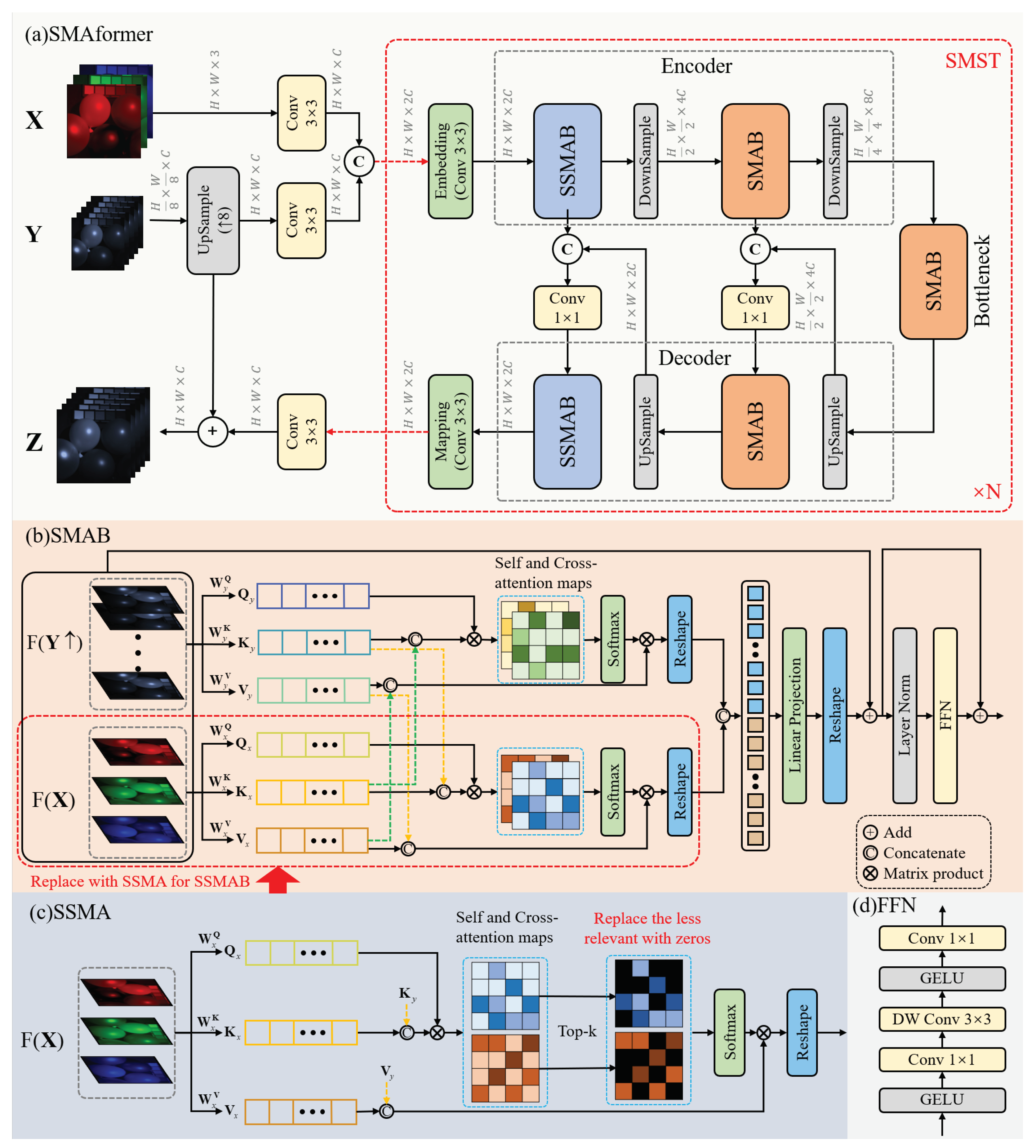
Perform the above-mentioned operations for each channel of , generating . Then, we feed and into separate convolutional layers to achieve the same shape. Following concatenation, the concatenated output is directed into N Single-stage Mixed Spectral-wise Transformer (SMST) modules. The SMST adopts a U-shaped structure consisting of an encoder, decoder, and bottleneck. The input is first passed through the mapping to obtain the initial features and . Considering the spatially sparse nature of HSIs, the first stage of the encoder utilizes Sparse Spectral Mix-Attention Blocks (SSMAB) at a high resolution, while the SMAB is used in the subsequent low-resolution stage and bottleneck. The same strategy is employed in the decoder. Both the embedding and mapping layers employ a convolutional layer, while downsampling uses a convolutional layer with a stride of 2. To minimize information loss during downsampling, skip connections are utilized between the encoder and decoder. Specifically, after upsampling through a convolutional layer, we acquire features at an identical resolution as the encoding step and subsequently concatenate them along the channels, and a convolution layer is employed for the dimensionality reduction as the input for the subsequent step. The output of the N SMST is further processed through a convolution layer to yield a feature matrix with the same dimensions as . Ultimately, this feature matrix is summed with to produce the final . The overall network structure can be expressed as the following formula:
where represents a convolution layer and indicates N SMST modules. We will provide a more detailed explanation of the SMAB and the sparse attention in the SSMAB in the next two sections.
3.2. Spectral Mix-Attention Block
Different from the previous use of one-stream and two-stream networks, our network employs a completely new architecture. The SMAB, as illustrated in Figure 2b, plays a crucial role in the system. It takes input features from and , extracting their long-range features simultaneously, and integrating the interactive information between them. This module differs from the traditional transformer in two key ways. First, taking into account the spatial sparseness and interspectral correlation in HSIs [34], we perform the attention operation on the image channels. This approach not only reduces the computational complexity but also proves to be more suitable for the current task. Second, we employ two parallel attention modules: self-attention and cross-attention. These modules not only focus on their own long-range information but also capture the cross-information between the two inputs. Specifically, we expand and along the channel dimension and apply linear transformations to obtain , , for and , , for . Then, we concatenate the and , as well as the and , and perform the attention operation by using their respective . This approach enables us to effectively capture not only the intrinsic relationships within and themselves but also the dynamic exchange of information between them. The following formula illustrates this process:
where , , and , , denote the learnable parameters of , , and of and , respectively; and denote the attention of and , respectively, which include self-attention and cross-attention. Subsequently, after concatenating the features obtained from the two pathways, we apply a linear projection, followed by reshaping it to match the same dimensions as the input. Linear projection can be expressed as the following formula:
where and represent the input and output features, respectively; represents the learnable parameters; and b represents bias. Finally, after the layer normal operation, it passes through the Feed Forward Neural Network (FFN), which is shown in Figure 2d.
3.3. Sparse Spectral Mix-Attention Block
The global self-attention of the transformer is not well-suited for MHIF. This is primarily due to two reasons. Firstly, HSIs exhibit spatial sparsity, making dense self-attention unsuitable for capturing their physical characteristics. Secondly, the spectral correlation in HSIs is stronger than the spatial correlation. Therefore, it is necessary to reduce the proportion of spatial-reference-information branches to mitigate the interference of irrelevant features and noise.
To overcome these limitations, We introduce a sparse-attention [35] module that leverages the sparsity inherent in neural networks, as shown in Figure 2c. This module is applied to the branch of MSI and integrated into the overall framework. The initial feature-extraction stage and the acquisition of , , remain consistent with the SMAB. However, after calculating the , we select only the Top-k elements with the largest attention coefficients in the attention map. Here, the value of Top-k is an adjustable dynamic parameter, and we extract the largest portion of data from the attention map; for instance, or . Other small values are replaced with zeros. Then, these processed attention maps are individually multiplied by a learnable parameter. Subsequently, we take the average of these results to derive the final attention map. The objective of this step is to retain the most important components and discard redundant or irrelevant ones. The final formulation for sparse attention will take the following form:
where is an operator that selects the Top-k values; it can be represented by the following formula:
where is the k-th largest value in the j-th row of .
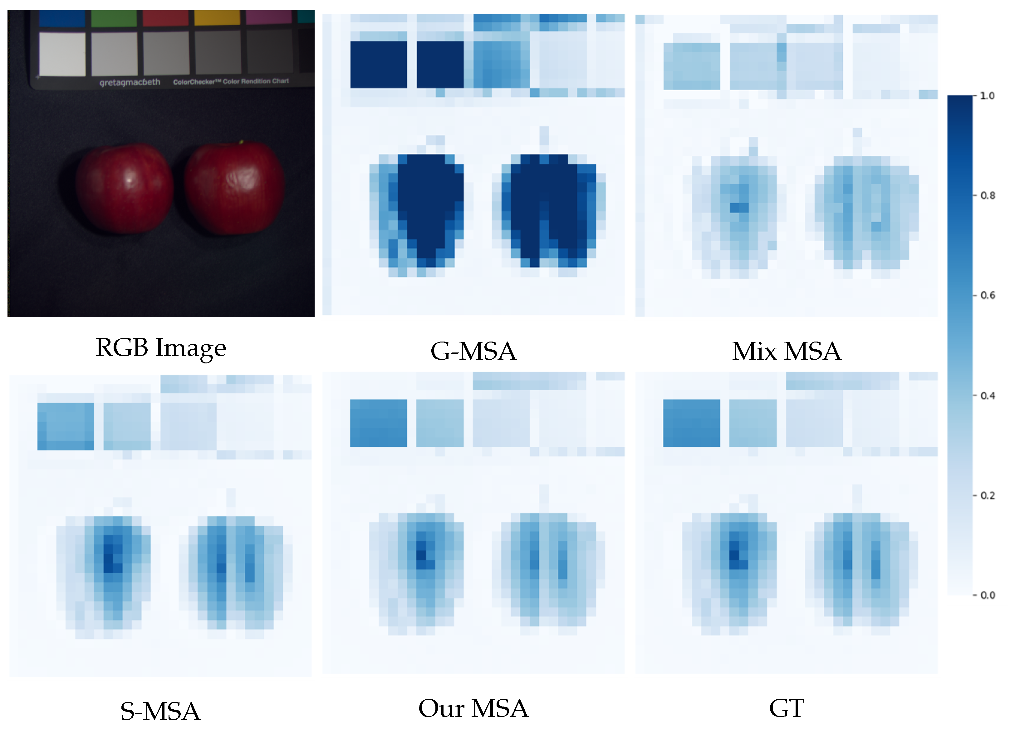
After applying this method in the HR step, the rest of the process is always the same as the previous method. We selected real and fake apples from the CAVE dataset [36] and plotted the correlation coefficients of the 20th spectral band in the HSI. Figure 3 illustrates the impact of employing various multihead self-attention (MSA) techniques, i.e., the original global MSA (G-MSA) [37], Mix MSA [38], Spectral MSA (S-MSA) [34], and our MSA. It is evident that the heat map generated through our utilization strategy exhibits the highest resemblance to the Ground Truth (GT).
3.4. Loss Function
After obtaining the reconstructed HR-HSI, we proceed to train the network by using the following loss-function formula:
The loss function comprises two components: the first component is the loss function, aimed at enhancing the clarity of the recovered edges and details. The formula is as follows:
where and denote the GT and the fusion result, respectively.
The second component is the loss function [39], which contributes to the overall image performance improvements. It is defined as
where p represents different bands from 1 to S, and S represents the number of channels of the image. and represent the average values of the GT and the fusion result, respectively, while and signify the standard deviation of the image pixel values. represents covariance, and and are two constants introduced to prevent a denominator of 0; and take the values and , respectively. The parameter in the middle serves as a coefficient used to balance the two components, and in this paper, a value of is employed.
4. Experiments
In this section, to demonstrate the effectiveness of the method presented in this paper, we carried out a series of experiments. Firstly, we introduce the experimental environment and configuration, as well as present three datasets and various evaluation metrics. Following this, a comprehensive comparative analysis is performed to assess the performance of the method proposed in this paper in comparison to several advanced methods on these datasets. Finally, in order to validate the efficacy of our proposed module, we conducted ablation experiments
4.1. Experimental Setup and Model Details
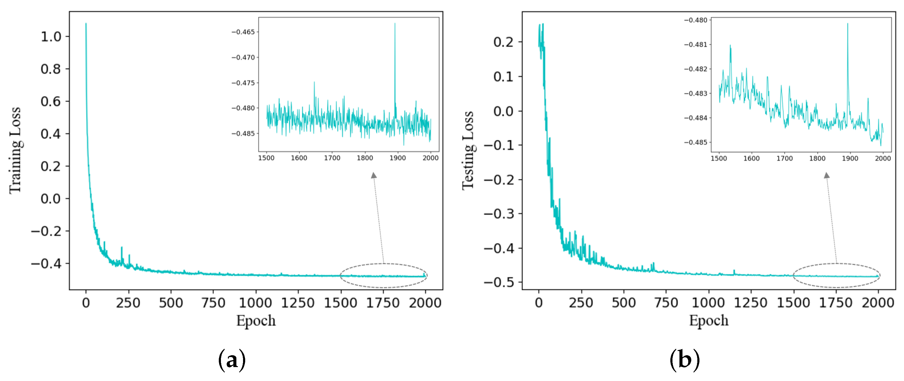
This method utilizes PyTorch 1.10.1 and Python 3.6.15 for training on a single NVIDIA GPU GeForce GTX 2080Ti. The Adam optimizer is employed to minimize the loss function, and for the learning rate, a dynamic approach is adopted. Initially, the learning rate is set to 1 × 10⁻⁴ and then decreased by a factor of 0.8 every 100 epochs. Based on the initial configuration outlined above, we conducted experiments by using the CAVE dataset and generated curves illustrating the relationship between the training loss, testing loss, and epochs in Figure 4. As the decrease in the loss function gradually plateaus in the later stages, we introduced an enlarged image specifically focusing on the epoch range from 1500 to 2000 in the upper right corner.
It is evident that both training and testing losses experienced a substantial decline within the initial 250 epochs. However, during the subsequent phases, the rate of decline decelerated. The enlarged images provide further insight, indicating occasional fluctuations in the middle epochs; nevertheless, the overarching trend remains downward, reassuringly indicating an absence of overfitting within this specified range. Despite these positive observations, we opted for a training epoch limit of 2000, considering the pragmatic constraint of time.
4.2. Datasets
To fully validate the effectiveness of the method proposed in this paper, we conducted a comparison by using three synthetic benchmark datasets, including two real-world datasets: CAVE [36] and Harvard [40], and a remote-sensing dataset: Pavia Center. The characteristics of these datasets are as follows:
CAVE: Captured by an Apogee Alta U260 CCD camera, this dataset comprises spectral bands ranging from 400 nm to 700 nm with 10 nm intervals, representing real-world objects. It consists of a total of 32 scenes, categorized into five groups: Stuff, Skin and Hair, Paints, Food and Drinks, and Real and Fake. Each scene contains 512 × 512 pixels and 31 spectral bands. Additionally, RGB images corresponding to these scenes are also provided. For our experiments, we selected the first 20 scenes as the training set and the remaining 12 scenes as the test set.
Harvard: Captured by using Nuance FX, CRI Inc., this dataset comprises both indoor and outdoor real scenes captured under sunlight. It contains the same 31 spectral bands as the CAVE dataset, but the spectral band ranges from 420 nm to 720 nm. The resolution of each scene is 1392 × 1040 pixels. We designated the last 12 scenes as the test set and used the remaining scenes for training.
Pavia Center: The Pavia Center dataset was obtained through satellite remote sensing by using ROSIS sensors, capturing imagery from the heart of Pavia, Italy. Pavia is a small city encompassing urban regions, agricultural land, and diverse geographic features, and the scenes are even more intricate. This dataset comprises 102 spectral bands, and the images have a resolution of 1096 × 1096 pixels.
Data Simulation: For the CAVE and Harvard datasets, to train the network, paired LR-HSI and HR-MSI data are required. However, the dataset only provides one HSI image, necessitating data simulation. In this process, the original image serves as the GT. The HR-MSI image is calculated by using the response function of the Nikon D700 camera and the original HSI image. For LR-HSI, a Gaussian convolution kernel with size r × r is applied to blur the original HSI image. The resulting image is then downsampled by a factor of eight, yielding the final LR-HSI. Due to the Pavia Center dataset consisting of only a single image, it was divided into two segments. The 512 × 216 pixel block located in the lower left corner serves as the test set while the remaining sections are allocated for training. The HR-MSI was generated by utilizing the spectral response functions of the IKONOS satellite and raw images. The method used to generate the LR-HSI remains consistent with the previous two methods.
4.3. Evaluation Metrics
To comprehensively assess the efficacy of our method, we chose five evaluation metrics to appraise the images restored by our approach. These metrics include PSNR, the Structural Similarity Index Metric (SSIM) [39], the Spectral Angle Mapper (SAM) [41], Erreur Relative Global Adimensionnelle Synthese (ERGAS) [42], and the Universal Image-Quality Index (UIQI) [43]. Subsequently, we will introduce each of these evaluation indicators individually.
4.3.1. PSNR
PSNR calculates the peak error between the corresponding pixels of the generated image and the reference image. The formula for this calculation is as follows:
where p represents different bands from 1 to S, and S represents the number of channels of the image. represents the maximum pixel value of the two input images, with the maximum value for the images in this paper being one. stands for the Mean Square Error between the GT and the fusion result, and its formula is as follows:
where H and W represent the height and width of the image, respectively. A higher PSNR value indicates a smaller error between the generated image and the real image, indicating better image quality.
4.3.2. SSIM
The SSIM measures the similarity between two images, focusing on improved image quality in terms of brightness, contrast, and structure. The calculation formula is as follows:
where and represent the average values of the image pixels, serving to quantify image brightness, while and signify the standard deviation of the image pixel values, used to gauge the image contrast. represents covariance, indicating the similarity in image structure, and and are two constants introduced to prevent a denominator of 0; and take the values and , respectively. This metric aligns more closely with human-visual-perception characteristics than PSNR. A larger SSIM value corresponds to a better human-visual-perception effect and a smaller disparity between the enhanced image and the original image.
4.3.3. SAM
The SAM treats the spectrum of each pixel within the image as a high-dimensional vector and quantifies the similarity between these spectra by determining the angle between the two vectors. A smaller angle indicates a higher degree of similarity between the two spectra. The formula for the SAM is expressed as follows:
4.3.4. ERGAS
ERGAS is a metric used to assess the quality of remote-sensing images. It is typically employed to compare the quality difference between two remote-sensing images. A lower ERGAS value indicates a smaller difference between the reconstructed image and the original image, indicating higher image quality. It is defined as follows:
where r represents the magnification of the image; the value of r is set to eight in this paper. represents the square of the mean value of the pixel value in the p-th spectral dimension of the image.
4.3.5. UIQI
The UIQI is a metric used to assess the quality of an image by comparing it to a reference or original image. It measures the similarity between the two images in terms of three key factors: the correlation loss, brightness distortion, and contrast distortion. The UIQI is a mathematical metric and does not explicitly consider the human visual system. However, it has been found to be consistent with subjective quality assessments for a wide range of image distortions. It is defined as follows:
The greater the UIQI value, the higher the quality of the corresponding image.
4.4. Quantitative Analysis
To demonstrate the effectiveness of our approach in this study, we conducted comprehensive experiments on two datasets. Furthermore, we compared our method with several state-of-the-art approaches, encompassing a variety of research methods, including matrix factorization-based LTTR [44], CNN-based MHF-Net [19], DBIN [45], ADMM-HFNet [20], Spf-Net [21], GuidedNet [46], and transformer-based Fusformer [24].
Table 1 provides an overview of the average quality metrics for our method and other methods on the CAVE dataset. It is evident that our method consistently claims the top position across all performance indicators. Specifically, in terms of the PSNR metric, we outperform the second-ranked method by 0.3 dB, signifying a more robust noise-suppression capability in our approach. Furthermore, in the SSIM metric, we also maintain a lead, indicating superior perceptual quality in the images generated by our method. In the realm of spectral recovery, our SAM score significantly surpasses that of the second-ranked method, resulting in minimal spectral distortion. Lastly, when considering the two comprehensive evaluation metrics, ERGAS and the UIQI, we maintain a substantial lead, underlining that the images restored by our method exhibit superior overall quality, closely resembling real-world images.
Similarly, Table 2 presents the performance metrics for our method and other methods on the Harvard dataset, where our method also excels across various indicators. Although we rank slightly lower than the first-place method in the SSIM and ERGAS metrics, we still maintain a significant lead over the third-place method. In all other metrics, we significantly outperform other methods.
In summary, our method showcases an exceptional performance in image-quality restoration, as demonstrated through evaluations on the CAVE and Harvard datasets. Whether it is the noise reduction, perceptual quality, spectral recovery, or overall image-quality assessment, our method consistently emerges as the leader in these domains, underscoring its remarkable potential in the field of MHIF.
4.5. Qualitative Analysis
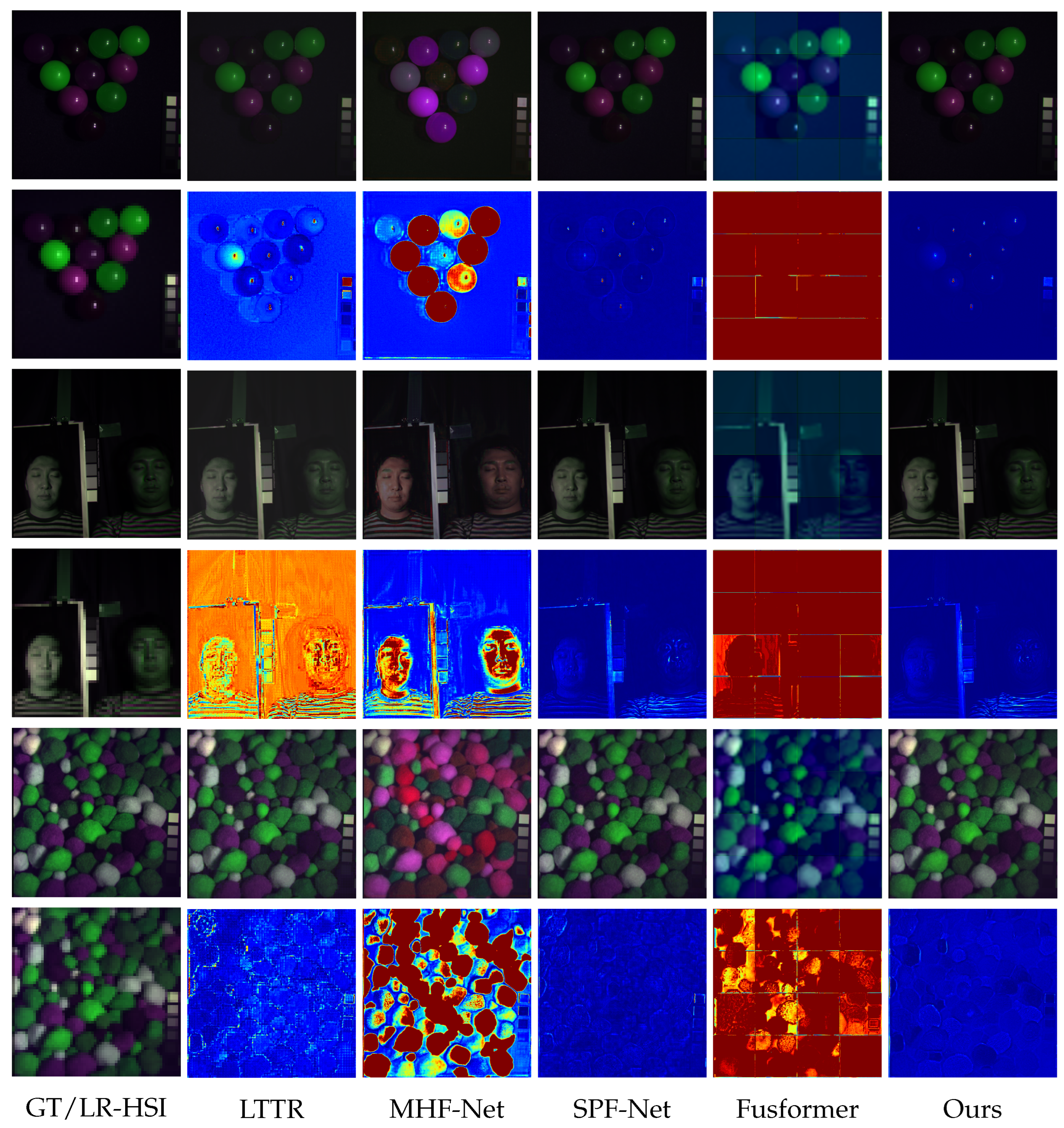
To better exhibit the effectiveness of our method, we conducted comparisons with four other four methods. In Figure 5, we chose three representative images from CAVE, each displaying its pseudo-RGB representation, utilizing the 3rd, 13th, and 2nd dimensions. The error maps below demonstrate their corresponding images; in the error map, a stronger blue color indicates that the image has fewer errors, while a stronger red color indicates that the image has more errors. From the figures, it is evident that MHF-net and Fusformer exhibit noticeable color deviations in their restored images, indicating significant spectral errors in the recovered HSI. This discrepancy is also apparent in their respective error maps when compared to the GT. LTTR performs better compared to the first two methods, yet still shows pronounced distortions in challenging areas, such as the colored spheres in the image. The SPF-net method yields relatively favorable results with overall minimal distortions and relatively realistic details.
In contrast, our method demonstrates the smallest difference when compared to the GT. In terms of color, our images exhibit no discernible differences, suggesting that our method preserves spectral information with minimal distortion. Furthermore, in terms of details, our method accurately restores the object structures, even in areas where other methods struggle to provide clear representations.
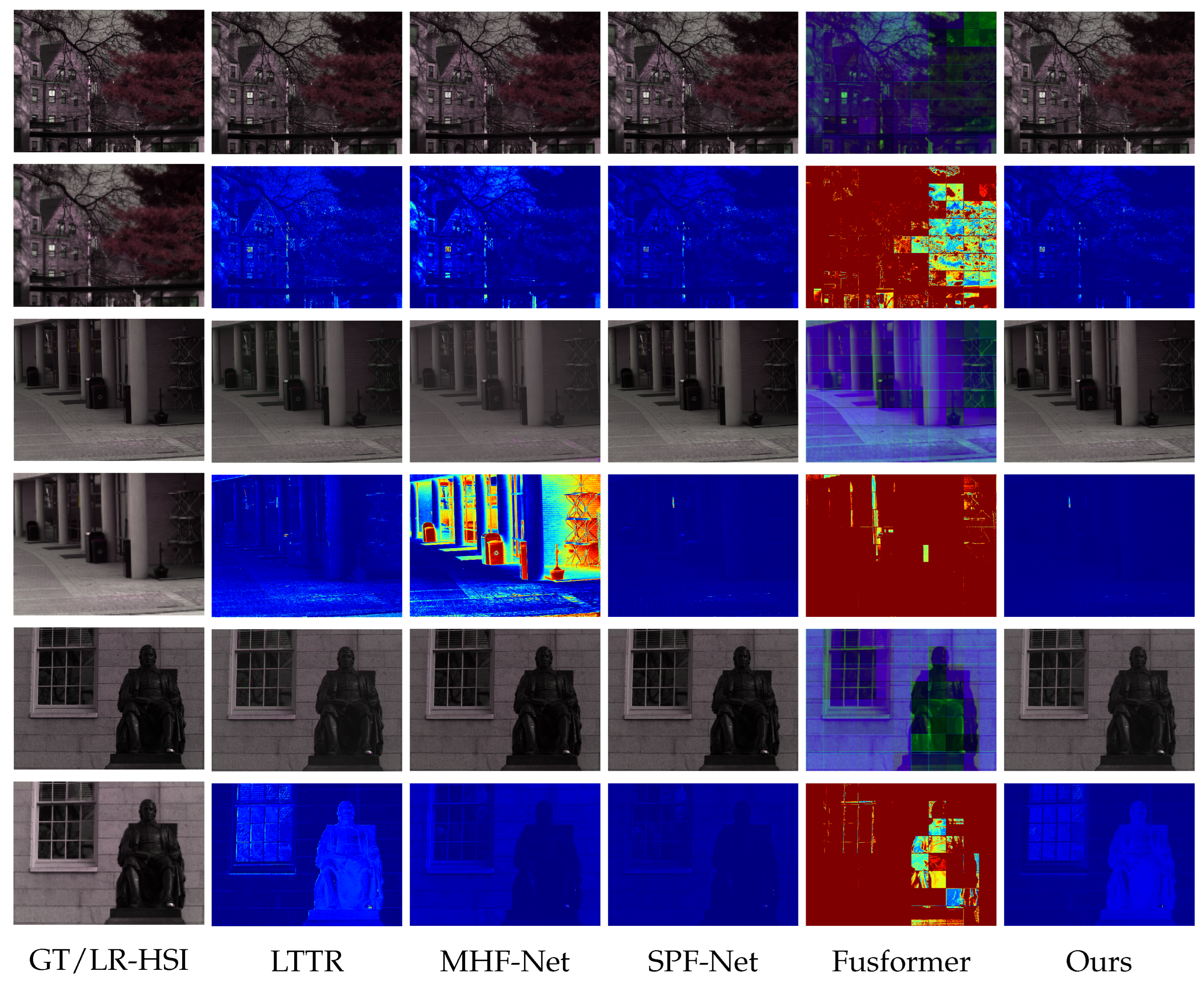
To provide a more comprehensive display of our restoration results, we conducted experiments by using the Harvard dataset. Figure 6 showcases the images restored by our method and the results of the other methods. It can be observed that MHF-net performs similarly to the CAVE dataset, with a better overall performance, but still exhibits notable spectral distortions in some images. The other three methods produce images with fewer distortions, although some deficiencies remain in certain details. Our method clearly outperforms the others both globally and locally, with hardly any evident errors in the error maps.
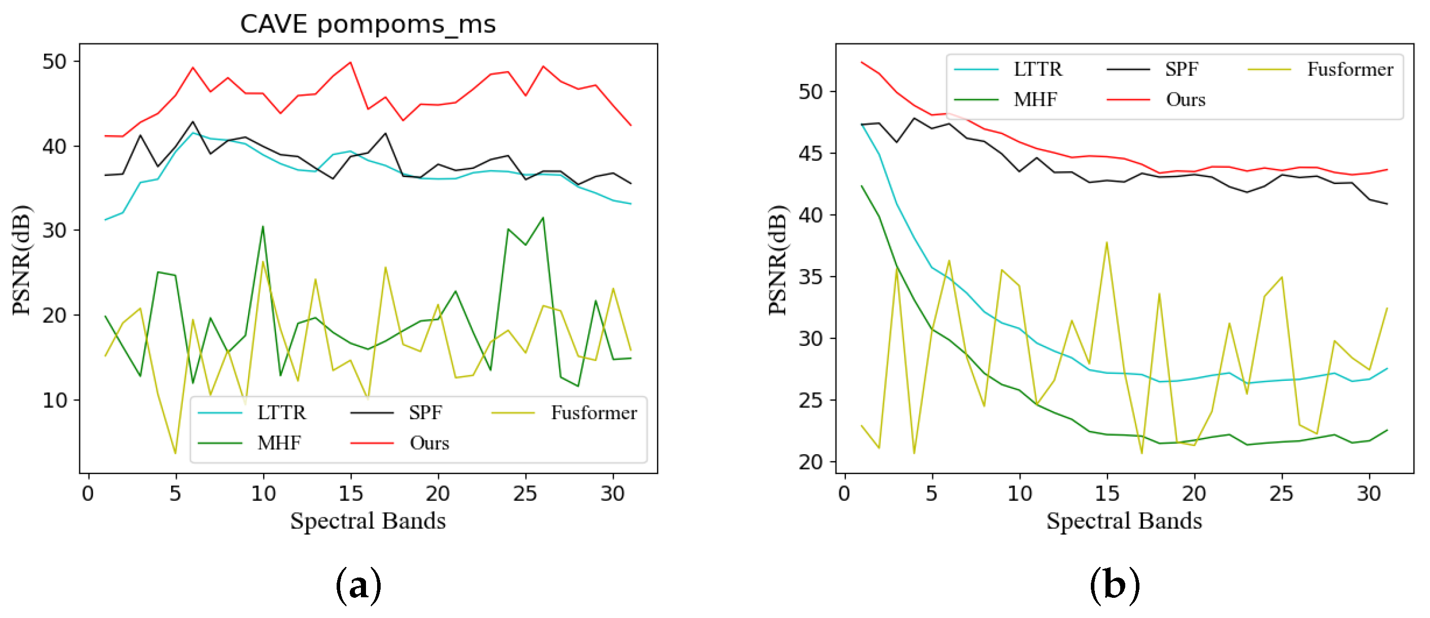
To showcase the superior performance of our method, we selected an image from both the CAVE and Harvard datasets. We then computed the PSNR values for each spectral dimension and visualized them in Figure 7. As Figure 7 demonstrates, our SMAformer method (depicted by the red curve) consistently outperforms other methods, clearly leading the pack. This indicates that our method not only excels in the overall image-recovery quality but also surpasses others in every spectral dimension.
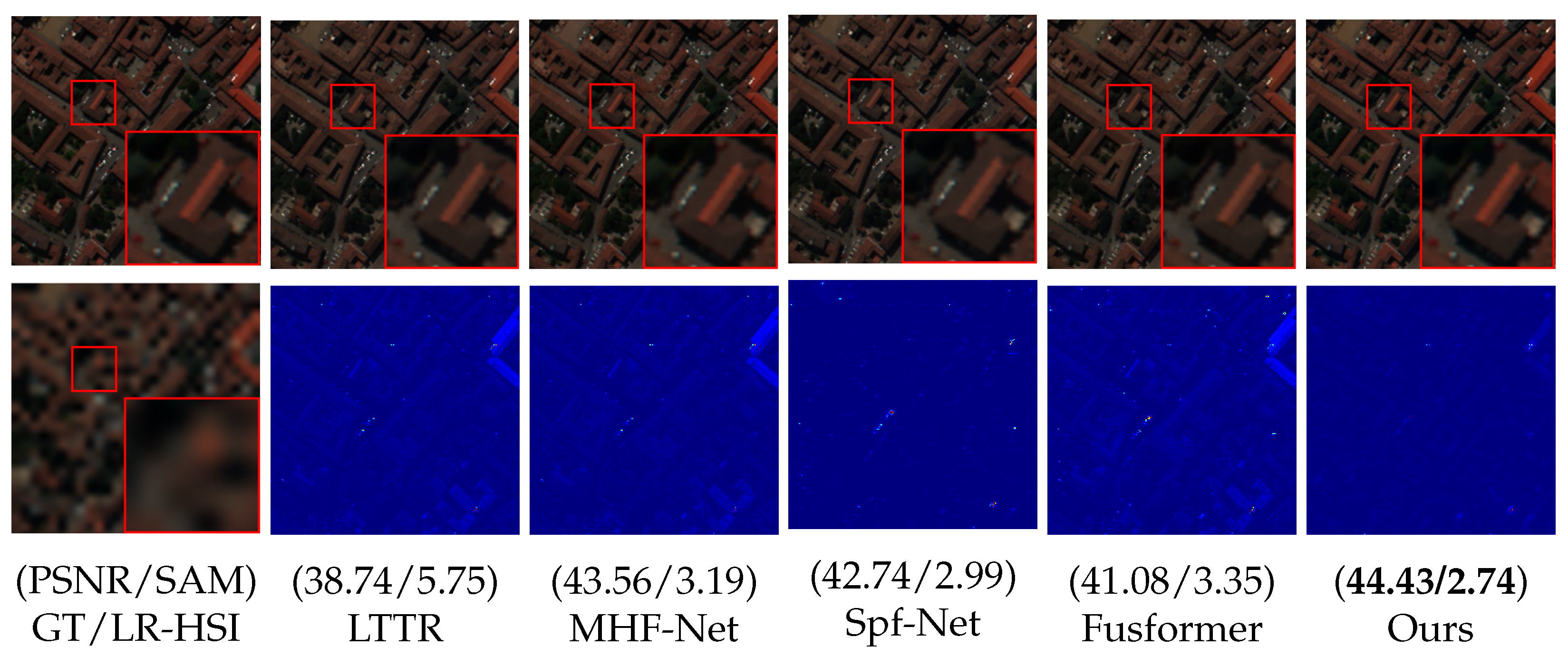
Furthermore, to validate the practicality of our approach, we conducted comparative experiments on real remote-sensing imagery from Pavia Center, and the results are shown in Figure 8. The resulting image depicts a 216 × 216 pixel section situated on top of the test set. We assigned the 65th band to red, the 30th band to green, and the 15th band to blue, creating a pseudo-RGB representation. To highlight details, we applied a magnification factor to a specific area by using a red box within the image. Additionally, error maps were generated and displayed beneath the respective pseudo-RGB image.
After a thorough image analysis, it is evident that the other four methods indeed produced satisfactory results, effectively revitalizing the original visual fidelity. Nevertheless, upon meticulous scrutiny of the magnified image, it becomes apparent that certain fine details have not been fully restored. Common issues such as chromatic aberration and blurred edges persist in their results. In stark contrast, our method excels in the meticulous restoration of these intricate details. From the error map, it is evident that there is virtually no distinction between our method and the actual image. Our approach adeptly and precisely rejuvenates the true appearance, achieving the highest scores across various performance indicators.
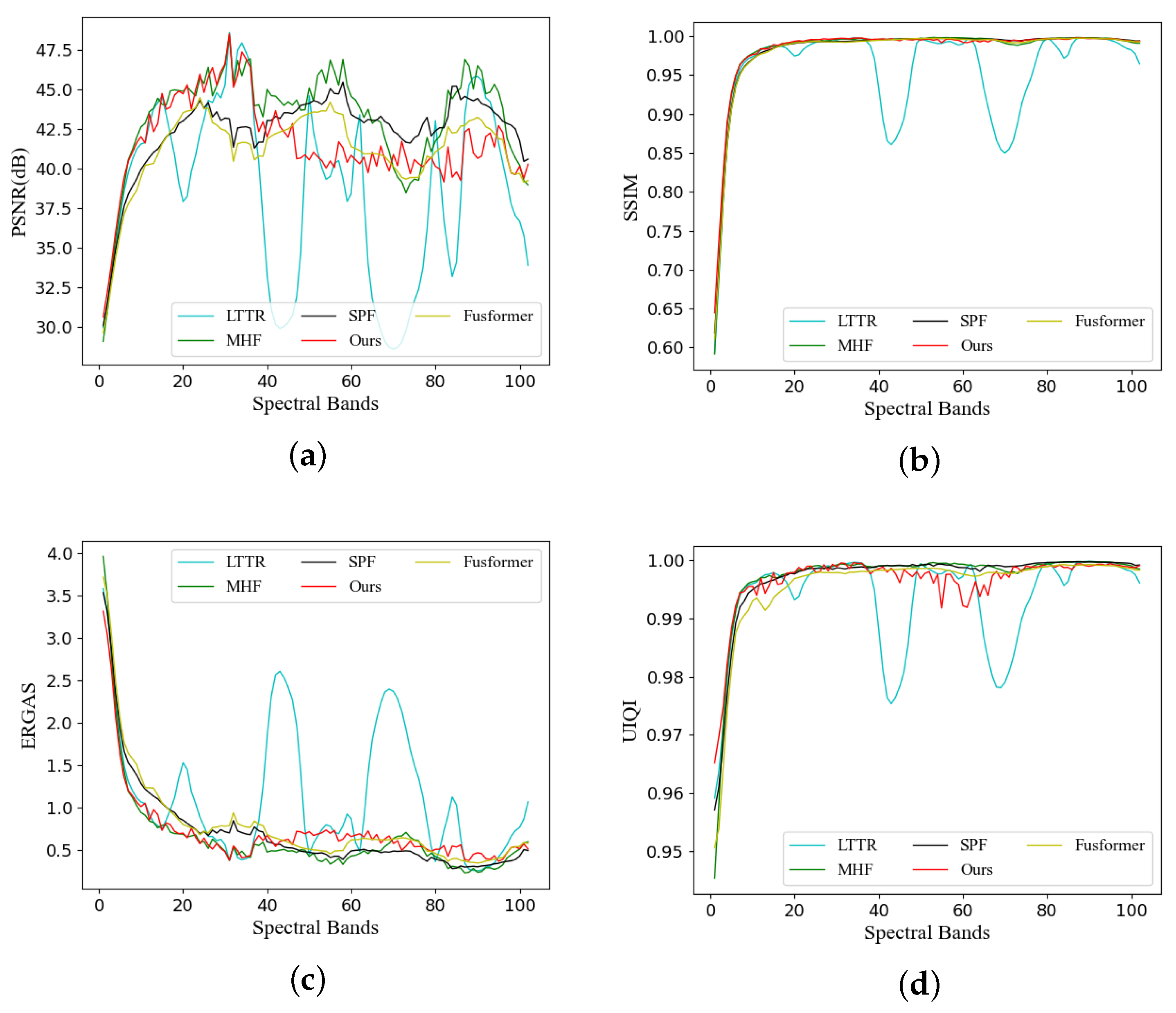
In Figure 9, we present the index curves representing images generated by different methods alongside the GT in each spectral band. Figure 9a illustrates the PSNR values. It is evident that our method excels in lower spectral bands and still delivers a strong performance in higher dimensions, even though there is a slight decline. This demonstrates that images produced by our method exhibit reduced noise levels. Figure 9b showcases the performance based on the SSIM values. With the exception of the LTTR method, which exhibits significant fluctuations, the other methods maintain a relatively consistent performance. Figure 9c illustrates the performance of ERGAS curves across various dimensions. Our approach demonstrates excellent results in the middle and low bands, suggesting that the image quality restored by our method excels particularly in these bands. In Figure 9d, we observe the UIQI indicator. Our method lags slightly behind in the middle bands but consistently leads in other bands. This underlines the effectiveness of our approach in preserving the image quality across different spectral bands.
In summary, based on the performance on these three synthetic datasets, our method not only excels in terms of metrics but also produces more realistic images with richer detailed information.
4.6. Ablation Study
To validate the effectiveness of our proposed method, we conducted ablation studies by using the CAVE dataset.
Our primary module, the SMST, underwent a total of three repetitions. To determine the most appropriate number of repetitions, we conducted experiments, including one, two, three, and four repetitions. The results of experiments with different repetition numbers N on the CAVE dataset are presented in Table 3. From the table, it can be observed that increasing the repetition number N to a certain extent enhances the performance of the model. The SSIM and SAM metrics reached their peak results at . However, the PSNR, ERGAS, and UIQI metrics exhibited superior performance at . Simultaneously, with an increase in N, the parameters of the model also increased, leading to a significant extension in the time required for image generation. Therefore, to strike a balance between the performance metrics and generation time, we opted for three repetitions, i.e., . In this scenario, our model comprises 6.2 million learnable parameters and operates at a floating-point operations per second (FLOPS) rate of 330 billion. The average training duration for our model spans 22 h.
In this paper, we utilized two distinct loss functions, loss and loss, to optimize our model. To strike a balance between the effects of these two loss functions, we introduced a hyperparameter, denoted as . The purpose of this experiment is to systematically explore the impact of varying values 1, 0.5, 0.1, and 0.01 on the performance of the model and determine the most effective balancing configuration. Our model was trained from scratch by using the CAVE dataset, and the final experimental results are presented in Table 4. Based on the data presented in the table, it is evident that larger values of , such as 1 and , lead to convergence issues and adversely impact the final performance of the model. Conversely, when is set to a smaller value, such as 0.01, although acceptable results are achieved, the distinctive impact of the loss is not effectively demonstrated. Consequently, we carefully selected the optimal value of 0.1. This choice strikes a balance, avoiding convergence disruptions while still allowing the loss to exert its intended influence on the performance of the model.
We proposed two modules: the SMAB and SSMAB. The SMAB leverages the flexibility of the transformer to establish self-generated and mutual correlations between HR-MSIs and LR-HSIs within the module. The SSMAB builds upon the SMAB by incorporating a sparse-attention module to better accommodate the spatial sparse characteristics of HSIs. To assess the effectiveness of our proposed modules, we conducted experiments. We replaced the SMAB with residual convolutional blocks [47] in the original module to obtain the w/o SMAB method, and we replaced the SSMAB with the SMAB to create the w/o SSMAB method. While keeping the other parameters constant, the final results are presented in Table 5.
Table 5 reveals that substituting the SMAB with residual convolutional blocks led to a notable drop in PSNR by 2.18 dB. This suggests that our module excels in extracting crucial information from both images compared to its predecessors. When the SSMAB was omitted, the PSNR decreased by 1.54 dB, underscoring the idea that sparsity is better suited for handling HSIs.
5. Conclusions
In this paper, we proposed a novel model for the MHIF task called SMAformer. Different from previous fusion methods, we focused on fusion super-resolution tasks and gave full play to the flexibility of the transformer model. We designed a multistage fusion module that can effectively capture the information between space and the spectrum to improve the fusion effect. In addition, considering the characteristics of HSIs, we performed sparse processing inside the model to make the generated images more realistic. Extensive experimental results on three benchmark datasets demonstrated that our SMAformer surpassed the state-of-the-art methods.
Although we made significant progress in our current research, there are still challenges that need to be addressed. Firstly, supervised training requires a large number of paired high- and low-resolution images, which are not easily obtainable in real-world scenarios, especially in specific domains or applications. This limitation hinders the universality of our model. To tackle this dilemma, we plan to shift our research focus towards unsupervised MHIF tasks. This approach does not rely on precise paired data but instead depends on the self-learning of the model to enhance resolution. Research in this direction holds a distinct advantage in handling large-scale datasets lacking GT in real-world situations.
In our future work, we will also explore and incorporate advanced Generative Adversarial Networks (GANs) [48] and self-supervised learning techniques to improve the performance of the model in unsupervised environments. These methods can assist us in better capturing latent structures and features within images, thereby enhancing the effectiveness of the MHIF task.
Furthermore, we intend to optimize the generalization ability of the model to adapt to the HSI SR requirements in different environments and scenarios. By delving into the exploration of distinctive features in various domains, we aim to make the model more adaptable and versatile, better addressing challenges in practical applications.
Author Contributions
Conceptualization, S.Y.; methodology, S.Y.; software, S.Y.; validation, S.Y.; formal analysis, X.Z.; investigation, X.Z.; resources, H.S.; data curation, S.Y.; writing—original draft preparation, S.Y.; writing—review and editing, H.S. and X.Z.; visualization, S.Y.; supervision, H.S.; project administration, X.Z.; funding acquisition, X.Z. and H.S. All authors have read and agreed to the published version of the manuscript.
Funding
This work was supported in part by the Seventh Batch of Science and Technology Development Plan (Agriculture) Project of Suzhou (SNG2023007) and in part by the NSFC under Grant No. 61872189.
Data Availability Statement
Data are contained within the article.
Conflicts of Interest
The authors declare no conflicts of interest.
References
- Sun, L.; Zhao, G.; Zheng, Y.; Wu, Z. Spectral–spatial feature tokenization transformer for hyperspectral image classification. IEEE Trans. Geosci. Remote Sens. 2022, 60, 1–14. [Google Scholar] [CrossRef]
- Uzkent, B.; Hoffman, M.J.; Vodacek, A. Real-time vehicle tracking in aerial video using hyperspectral features. In Proceedings of the IEEE Conference on Computer Vision and Pattern Recognition Workshops, Las Vegas, NV, USA, 26 June–1 July 2016; pp. 36–44. [Google Scholar]
- Hong, D.; Yao, J.; Meng, D.; Xu, Z.; Chanussot, J. Multimodal GANs: Toward crossmodal hyperspectral–multispectral image segmentation. IEEE Trans. Geosci. Remote Sens. 2020, 59, 5103–5113. [Google Scholar] [CrossRef]
- Aiazzi, B.; Baronti, S.; Selva, M. Improving component substitution pansharpening through multivariate regression of MS + Pan data. IEEE Trans. Geosci. Remote Sens. 2007, 45, 3230–3239. [Google Scholar] [CrossRef]
- Chavez, P.; Sides, S.C.; Anderson, J.A. Comparison of three different methods to merge multiresolution and multispectral data- Landsat TM and SPOT panchromatic. Photogramm. Eng. Remote Sens. 1991, 57, 295–303. [Google Scholar]
- Burt, P.J.; Adelson, E.H. The Laplacian pyramid as a compact image code. In Readings in Computer Vision; Elsevier: Amsterdam, The Netherlands, 1987; pp. 671–679. [Google Scholar]
- Loncan, L.; De Almeida, L.B.; Bioucas-Dias, J.M.; Briottet, X.; Chanussot, J.; Dobigeon, N.; Fabre, S.; Liao, W.; Licciardi, G.A.; Simoes, M.; et al. Hyperspectral pansharpening: A review. IEEE Geosci. Remote Sens. Mag. 2015, 3, 27–46. [Google Scholar] [CrossRef]
- Starck, J.L.; Fadili, J.; Murtagh, F. The undecimated wavelet decomposition and its reconstruction. IEEE Trans. Image Process. 2007, 16, 297–309. [Google Scholar] [CrossRef]
- Bungert, L.; Coomes, D.A.; Ehrhardt, M.J.; Rasch, J.; Reisenhofer, R.; Schönlieb, C.B. Blind image fusion for hyperspectral imaging with the directional total variation. Inverse Probl. 2018, 34, 044003. [Google Scholar] [CrossRef]
- Akhtar, N.; Shafait, F.; Mian, A. Bayesian sparse representation for hyperspectral image super resolution. In Proceedings of the IEEE Conference on Computer Vision and Pattern Recognition, Boston, MA, USA, 7–12 June 2015; pp. 3631–3640. [Google Scholar]
- Dian, R.; Fang, L.; Li, S. Hyperspectral image super-resolution via non-local sparse tensor factorization. In Proceedings of the IEEE Conference on Computer Vision and Pattern Recognition, Honolulu, HI, USA, 21–26 July 2017; pp. 5344–5353. [Google Scholar]
- Li, S.; Dian, R.; Fang, L.; Bioucas-Dias, J.M. Fusing hyperspectral and multispectral images via coupled sparse tensor factorization. IEEE Trans. Image Process. 2018, 27, 4118–4130. [Google Scholar] [CrossRef]
- Kawakami, R.; Matsushita, Y.; Wright, J.; Ben-Ezra, M.; Tai, Y.W.; Ikeuchi, K. High-resolution hyperspectral imaging via matrix factorization. In Proceedings of the CVPR 2011, Colorado Springs, CO, USA, 20–25 June 2011; IEEE: Piscataway, NJ, USA, 2011; pp. 2329–2336. [Google Scholar]
- Akhtar, N.; Shafait, F.; Mian, A. Sparse spatio-spectral representation for hyperspectral image super-resolution. In Proceedings of the Computer Vision–ECCV 2014: 13th European Conference, Zurich, Switzerland, 6–12 September 2014; Proceedings, Part VII 13. Springer: Berlin/Heidelberg, Germany, 2014; pp. 63–78. [Google Scholar]
- Wei, Q.; Bioucas-Dias, J.; Dobigeon, N.; Tourneret, J.Y. Hyperspectral and multispectral image fusion based on a sparse representation. IEEE Trans. Geosci. Remote Sens. 2015, 53, 3658–3668. [Google Scholar] [CrossRef]
- Dong, C.; Loy, C.C.; He, K.; Tang, X. Learning a deep convolutional network for image super-resolution. In Proceedings of the Computer Vision–ECCV 2014: 13th European Conference, Zurich, Switzerland, 6–12 September 2014; Proceedings, Part IV 13. Springer: Berlin/Heidelberg, Germany, 2014; pp. 184–199. [Google Scholar]
- Dong, C.; Loy, C.C.; Tang, X. Accelerating the super-resolution convolutional neural network. In Proceedings of the Computer Vision–ECCV 2016: 14th European Conference, Amsterdam, The Netherlands, 11–14 October 2016; Proceedings, Part II 14. Springer: Berlin/Heidelberg, Germany, 2016; pp. 391–407. [Google Scholar]
- Palsson, F.; Sveinsson, J.R.; Ulfarsson, M.O. Multispectral and hyperspectral image fusion using a 3-D-convolutional neural network. IEEE Geosci. Remote Sens. Lett. 2017, 14, 639–643. [Google Scholar] [CrossRef]
- Xie, Q.; Zhou, M.; Zhao, Q.; Xu, Z.; Meng, D. MHF-Net: An interpretable deep network for multispectral and hyperspectral image fusion. IEEE Trans. Pattern Anal. Mach. Intell. 2020, 44, 1457–1473. [Google Scholar] [CrossRef]
- Shen, D.; Liu, J.; Wu, Z.; Yang, J.; Xiao, L. ADMM-HFNet: A matrix decomposition-based deep approach for hyperspectral image fusion. IEEE Trans. Geosci. Remote Sens. 2021, 60, 1–17. [Google Scholar] [CrossRef]
- Liu, J.; Shen, D.; Wu, Z.; Xiao, L.; Sun, J.; Yan, H. Patch-aware deep hyperspectral and multispectral image fusion by unfolding subspace-based optimization model. IEEE J. Sel. Top. Appl. Earth Obs. Remote Sens. 2022, 15, 1024–1038. [Google Scholar] [CrossRef]
- Yao, J.; Hong, D.; Chanussot, J.; Meng, D.; Zhu, X.; Xu, Z. Cross-attention in coupled unmixing nets for unsupervised hyperspectral super-resolution. In Proceedings of the Computer Vision–ECCV 2020: 16th European Conference, Glasgow, UK, 23–28 August 2020; Proceedings, Part XXIX 16. Springer: Berlin/Heidelberg, Germany, 2020; pp. 208–224. [Google Scholar]
- Yang, J.; Zhao, Y.Q.; Chan, J.C.W. Hyperspectral and multispectral image fusion via deep two-branches convolutional neural network. Remote Sens. 2018, 10, 800. [Google Scholar] [CrossRef]
- Hu, J.F.; Huang, T.Z.; Deng, L.J.; Dou, H.X.; Hong, D.; Vivone, G. Fusformer: A transformer-based fusion network for hyperspectral image super-resolution. IEEE Geosci. Remote Sens. Lett. 2022, 19, 1–5. [Google Scholar] [CrossRef]
- Jia, S.; Min, Z.; Fu, X. Multiscale spatial–spectral transformer network for hyperspectral and multispectral image fusion. Inf. Fusion 2023, 96, 117–129. [Google Scholar] [CrossRef]
- Cai, Y.; Lin, J.; Hu, X.; Wang, H.; Yuan, X.; Zhang, Y.; Timofte, R.; Van Gool, L. Coarse-to-fine sparse transformer for hyperspectral image reconstruction. In Proceedings of the European Conference on Computer Vision, Tel Aviv, Israel, 23–27 October 2022; Springer: Berlin/Heidelberg, Germany, 2022; pp. 686–704. [Google Scholar]
- Peng, J.; Sun, W.; Li, H.C.; Li, W.; Meng, X.; Ge, C.; Du, Q. Low-rank and sparse representation for hyperspectral image processing: A review. IEEE Geosci. Remote Sens. Mag. 2021, 10, 10–43. [Google Scholar] [CrossRef]
- Nunez, J.; Otazu, X.; Fors, O.; Prades, A.; Pala, V.; Arbiol, R. Multiresolution-based image fusion with additive wavelet decomposition. IEEE Trans. Geosci. Remote Sens. 1999, 37, 1204–1211. [Google Scholar] [CrossRef]
- Yokoya, N.; Yairi, T.; Iwasaki, A. Coupled nonnegative matrix factorization unmixing for hyperspectral and multispectral data fusion. IEEE Trans. Geosci. Remote Sens. 2011, 50, 528–537. [Google Scholar] [CrossRef]
- Zhang, K.; Wang, M.; Yang, S.; Jiao, L. Spatial–spectral-graph-regularized low-rank tensor decomposition for multispectral and hyperspectral image fusion. IEEE J. Sel. Top. Appl. Earth Obs. Remote Sens. 2018, 11, 1030–1040. [Google Scholar] [CrossRef]
- Xu, Y.; Wu, Z.; Chanussot, J.; Wei, Z. Hyperspectral images super-resolution via learning high-order coupled tensor ring representation. IEEE Trans. Neural Netw. Learn. Syst. 2020, 31, 4747–4760. [Google Scholar] [CrossRef]
- Dian, R.; Li, S.; Guo, A.; Fang, L. Deep hyperspectral image sharpening. IEEE Trans. Neural Netw. Learn. Syst. 2018, 29, 5345–5355. [Google Scholar] [CrossRef]
- Keys, R. Cubic convolution interpolation for digital image processing. IEEE Trans. Acoust. Speech Signal Process. 1981, 29, 1153–1160. [Google Scholar] [CrossRef]
- Cai, Y.; Lin, J.; Hu, X.; Wang, H.; Yuan, X.; Zhang, Y.; Timofte, R.; Van Gool, L. Mask-guided spectral-wise transformer for efficient hyperspectral image reconstruction. In Proceedings of the IEEE/CVF Conference on Computer Vision and Pattern Recognition, New Orleans, LA, USA, 18–24 June 2022; pp. 17502–17511. [Google Scholar]
- Chen, X.; Li, H.; Li, M.; Pan, J. Learning A Sparse Transformer Network for Effective Image Deraining. In Proceedings of the IEEE/CVF Conference on Computer Vision and Pattern Recognition, Vancouver, BC, Canada, 17–24 June 2023; pp. 5896–5905. [Google Scholar]
- Yasuma, F.; Mitsunaga, T.; Iso, D.; Nayar, S.K. Generalized assorted pixel camera: Postcapture control of resolution, dynamic range, and spectrum. IEEE Trans. Image Process. 2010, 19, 2241–2253. [Google Scholar] [CrossRef]
- Vaswani, A.; Shazeer, N.; Parmar, N.; Uszkoreit, J.; Jones, L.; Gomez, A.N.; Kaiser, Ł.; Polosukhin, I. Attention is all you need. In Proceedings of the 31st International Conference on Neural Information Processing Systems, Long Beach, CA, USA, 4–9 December 2017. Volume 30. [Google Scholar] [CrossRef]
- Cui, Y.; Jiang, C.; Wang, L.; Wu, G. Mixformer: End-to-end tracking with iterative mixed attention. In Proceedings of the IEEE/CVF Conference on Computer Vision and Pattern Recognition, New Orleans, LA, USA, 18–24 June 2022; pp. 13608–13618. [Google Scholar]
- Wang, Z.; Bovik, A.C.; Sheikh, H.R.; Simoncelli, E.P. Image quality assessment: From error visibility to structural similarity. IEEE Trans. Image Process. 2004, 13, 600–612. [Google Scholar] [CrossRef]
- Chakrabarti, A.; Zickler, T. Statistics of real-world hyperspectral images. In Proceedings of the CVPR 2011, Colorado Springs, CO, USA, 20–25 June 2011; IEEE: Piscataway, NJ, USA, 2011; pp. 193–200. [Google Scholar]
- Yuhas, R.H.; Goetz, A.F.; Boardman, J.W. Discrimination among semi-arid landscape endmembers using the spectral angle mapper (SAM) algorithm. In Proceedings of the JPL, Summaries of the Third Annual JPL Airborne Geoscience Workshop, Pasadena, CA, USA, 1–5 June 1992; AVIRIS Workshop. Volume 1. [Google Scholar]
- Wald, L. Quality of high resolution synthesised images: Is there a simple criterion? In Proceedings of the Third Conference Fusion of Earth Data: Merging Point Measurements, Raster Maps and Remotely Sensed Images, Sophia Antipolis, France, 26–28 January 2000; SEE/URISCA. pp. 99–103. [Google Scholar]
- Wang, Z.; Bovik, A.C. A universal image quality index. IEEE Signal Process. Lett. 2002, 9, 81–84. [Google Scholar] [CrossRef]
- Dian, R.; Li, S.; Fang, L. Learning a low tensor-train rank representation for hyperspectral image super-resolution. IEEE Trans. Neural Netw. Learn. Syst. 2019, 30, 2672–2683. [Google Scholar] [CrossRef]
- Wang, W.; Zeng, W.; Huang, Y.; Ding, X.; Paisley, J. Deep blind hyperspectral image fusion. In Proceedings of the IEEE/CVF International Conference on Computer Vision, Seoul, Repulic of Korea, 27–28 October 2019; pp. 4150–4159. [Google Scholar]
- Ran, R.; Deng, L.J.; Jiang, T.X.; Hu, J.F.; Chanussot, J.; Vivone, G. GuidedNet: A general CNN fusion framework via high-resolution guidance for hyperspectral image super-resolution. IEEE Trans. Cybern. 2023, 53, 4148–4161. [Google Scholar] [CrossRef]
- He, K.; Zhang, X.; Ren, S.; Sun, J. Deep Residual Learning for Image Recognition. In Proceedings of the 2016 IEEE Conference on Computer Vision and Pattern Recognition (CVPR), Las Vegas, NV, USA, 27–30 June 2016; pp. 770–778. [Google Scholar] [CrossRef]
- Goodfellow, I.; Pouget-Abadie, J.; Mirza, M.; Xu, B.; Warde-Farley, D.; Ozair, S.; Courville, A.; Bengio, Y. Generative Adversarial Nets. In Advances in Neural Information Processing Systems; Ghahramani, Z., Welling, M., Cortes, C., Lawrence, N., Weinberger, K., Eds.; Curran Associates, Inc.: Red Hook, NY, USA, 2014; Volume 27. [Google Scholar]
Figure 1.
Comparing two existing deep learning frameworks [20,21,22,23] with our SMAformer. The previous methods (a,b) solely focused on either spatial or spectral fusion, neglecting the spatial sparsity in HSI images. In contrast, our SMAformer (c) fully integrates both spatial and spectral information and incorporates sparse representation in spatial domains. Note that , , and indicate the Query (Q), key (K), and value (V) of *, respectively.

Figure 2.
Illustration of the proposed method. (a) The network architecture of our work, and (b) the structure of the SMAB. (c) A detailed description of the Sparse Spectral Mix Attention (SSMA). (d) Detailed description of the FFN. Note that the SSMAB is configured with 1 head, the SMAB following it has 2 heads, and there are 4 heads in the bottleneck.

Figure 3.
Comparison of spatial correlation among HSIs reconstructed by different MSAs. The image illustrates the correlation coefficients of the twentieth band in HSI. It is evident that the MSA strategy employed in our approach yields a correlation coefficient map that closely aligns with those of the GT.

Figure 4.
Curves of training loss and testing loss across epochs on CAVE dataset. (a) The training loss curve and (b) the testing loss curve.
Figure 4.
Curves of training loss and testing loss across epochs on CAVE dataset. (a) The training loss curve and (b) the testing loss curve.

Figure 5.
Comparison of results for three images in the CAVE dataset. Superballs in the first and second rows, pompoms in the third and fourth rows, and photo and face in the fifth and sixth rows. In each group of photos, the first column: the top/bottom image indicates the GT/corresponding LR-HSI in pseudocolor (R-3, G-13, and B-2), and the 2nd–6th columns are the visualization images and the corresponding error maps of all compared models [19,21,24,44].

Figure 6.
Comparison of results for three images in pseudocolor (R-29, G-21, and B-28) in the Harvard dataset [19,21,24,44].

Figure 7.
Comparison of PSNR index curves of different methods. The figure illustrates the PSNR values of each spectral band for images restored by using various methods in comparison to real images. (a) illustrates the results for pompoms_ms in the CAVE dataset, while (b) presents the results for Imageb9 in the Harvard dataset.

Figure 8.
Comparison of results of different methods on the Pavia Center dataset. First column: the top/bottom image indicates the GT/corresponding LR-HSI of the top 216 × 216-pixel test image from the Pavia Center dataset in pseudocolor (R-65, G-30, and B-15). The 2nd-6th columns: the visualization images and the corresponding error maps of all compared models. In the pseudocolor images, a red-marked region was triple magnified to assist the visual analysis [19,21,24,44].

Figure 9.
Comparison of indicator curves of different methods in the Pavia Center dataset. (a) The PSNR curve, (b) the SSIM curve, (c) the ERGAS curve, and (d) the UIQI curve.
Figure 9.
Comparison of indicator curves of different methods in the Pavia Center dataset. (a) The PSNR curve, (b) the SSIM curve, (c) the ERGAS curve, and (d) the UIQI curve.


Table 1.
Average quantitative results by all the compared methods on the CAVE testing set.
| Title | PSNR↑ | SSIM ↑ | SAM↓ | ERGAS↓ | UIQI↑ |
|---|---|---|---|---|---|
| LTTR [44] | 41.20 | 0.980 | 4.25 | 1.90 | 0.984 |
| MHFnet [19] | 45.23 | 0.988 | 4.88 | 0.71 | 0.981 |
| DBIN [45] | 45.02 | 0.981 | 3.38 | 0.71 | 0.992 |
| ADMM-HFNet [20] | 45.48 | 0.992 | 3.39 | 0.71 | 0.992 |
| SpfNet [21] | 46.29 | 0.990 | 4.24 | 1.46 | 0.980 |
| Fusformer [24] | 42.18 | 0.993 | 3.07 | 1.25 | 0.992 |
| GuidedNet [46] | 45.41 | 0.991 | 4.03 | 0.97 | - |
| Ours | 46.56 | 0.994 | 2.92 | 0.64 | 0.995 |
The best values are highlighted, and the second-best values are underlined. ↑ signifies better performance as the corresponding metric values increase, while ↓ indicates enhanced performance with decreasing metric values.
Table 2.
Average quantitative results by all the compared methods on the Harvard testing set.
| Title | PSNR↑ | SSIM ↑ | SAM↓ | ERGAS↓ | UIQI↑ |
|---|---|---|---|---|---|
| LTTR [44] | 40.06 | 0.999 | 4.69 | 1.29 | 0.993 |
| MHFnet [19] | 44.50 | 0.981 | 3.68 | 1.21 | 0.991 |
| DBIN [45] | 45.33 | 0.983 | 3.04 | 1.09 | 0.995 |
| ADMM-HFNet [20] | 45.53 | 0.983 | 3.04 | 1.08 | 0.995 |
| SpfNet [21] | 45.09 | 0.984 | 2.31 | 0.65 | 0.997 |
| Fusformer [24] | 41.96 | 0.995 | 3.33 | 2.86 | 0.995 |
| GuidedNet [46] | 41.64 | 0.981 | 2.85 | 1.20 | - |
| Ours | 47.86 | 0.995 | 2.25 | 0.75 | 0.997 |
The best values are highlighted, and the second-best values are underlined. ↑ signifies better performance as the corresponding metric values increase, while ↓ indicates enhanced performance with decreasing metric values.
Table 3.
Average quantitative results by different N on the CAVE testing set.
| N | PSNR↑ | SSIM ↑ | SAM↓ | ERGAS↓ | UIQI↑ | Time↓ |
|---|---|---|---|---|---|---|
| 1 | 43.06 | 0.986 | 3.69 | 1.19 | 0.993 | 0.45 |
| 2 | 45.38 | 0.990 | 3.20 | 0.97 | 0.991 | 0.51 |
| 3 | 46.56 | 0.994 | 2.92 | 0.64 | 0.995 | 0.55 |
| 4 | 46.01 | 0.995 | 2.91 | 0.78 | 0.993 | 0.68 |
The best values are highlighted. ↑ signifies better performance as the corresponding metric values increase, while ↓ indicates enhanced performance with decreasing metric values.
Table 4.
Average quantitative results by different on the CAVE testing set.
| PSNR↑ | SSIM ↑ | SAM↓ | ERGAS↓ | UIQI↑ | |
|---|---|---|---|---|---|
| 1 | 42.13 | 0.920 | 4.12 | 1.67 | 0.986 |
| 44.25 | 0.986 | 3.49 | 1.03 | 0.990 | |
| 46.56 | 0.994 | 2.92 | 0.64 | 0.995 | |
| 45.21 | 0.992 | 3.03 | 0.66 | 0.994 |
The best values are highlighted. ↑ signifies better performance as the corresponding metric values increase, while ↓ indicates enhanced performance with decreasing metric values.
Table 5.
Average quantitative results by different modules on the CAVE testing set.
| Method | PSNR↑ | SSIM ↑ | SAM↓ | ERGAS↓ | UIQI↑ |
|---|---|---|---|---|---|
| w/o SMAB | 44.38 | 0.991 | 3.24 | 0.96 | 0.990 |
| w/o SSMAB | 45.02 | 0.990 | 2.96 | 0.77 | 0.992 |
| Ours | 46.56 | 0.994 | 2.92 | 0.64 | 0.995 |
The best values are highlighted. ↑ signifies better performance as the corresponding metric values increase, while ↓ indicates enhanced performance with decreasing metric values.
Disclaimer/Publisher’s Note: The statements, opinions and data contained in all publications are solely those of the individual author(s) and contributor(s) and not of MDPI and/or the editor(s). MDPI and/or the editor(s) disclaim responsibility for any injury to people or property resulting from any ideas, methods, instructions or products referred to in the content. |
© 2023 by the authors. Licensee MDPI, Basel, Switzerland. This article is an open access article distributed under the terms and conditions of the Creative Commons Attribution (CC BY) license (https://creativecommons.org/licenses/by/4.0/).
Share and Cite
MDPI and ACS Style
Yu, S.; Zhang, X.; Song, H. Sparse Mix-Attention Transformer for Multispectral Image and Hyperspectral Image Fusion. Remote Sens. 2024, 16, 144. https://doi.org/10.3390/rs16010144
AMA Style
Yu S, Zhang X, Song H. Sparse Mix-Attention Transformer for Multispectral Image and Hyperspectral Image Fusion. Remote Sensing. 2024; 16(1):144. https://doi.org/10.3390/rs16010144
Chicago/Turabian StyleYu, Shihai, Xu Zhang, and Huihui Song. 2024. "Sparse Mix-Attention Transformer for Multispectral Image and Hyperspectral Image Fusion" Remote Sensing 16, no. 1: 144. https://doi.org/10.3390/rs16010144
Note that from the first issue of 2016, this journal uses article numbers instead of page numbers. See further details here.