
Fast and Accurate Hyperspectral Image Classification with Window Shape Adaptive Singular Spectrum Analysis

1
Changchun Institute of Optics, Fine Mechanics and Physics, Chinese Academy of Sciences (CIOMP), Changchun 130033, China
2
University of Chinese Academy of Sciences, Beijing 100049, China
3
School of Instrumentation and Optoelectronic Engineering, Beihang University, Beijing 100191, China
*
Author to whom correspondence should be addressed.
Remote Sens. 2024, 16(1), 81; https://doi.org/10.3390/rs16010081
Submission received: 2 October 2023
/
Revised: 11 December 2023
/
Accepted: 13 December 2023
/
Published: 25 December 2023
Abstract
:Hyperspectral classification is a task of significant importance in the field of remote sensing image processing, with attaining high precision and rapid classification increasingly becoming a research focus. The classification accuracy depends on the degree of raw HSI feature extraction, and the use of endless classification methods has led to an increase in computational complexity. To achieve high accuracy and fast classification, this study analyzes the inherent features of HSI and proposes a novel spectral–spatial feature extraction method called window shape adaptive singular spectrum analysis (WSA-SSA) to reduce the computational complexity of feature extraction. This method combines similar pixels in the neighborhood to reconstruct every pixel in the window, and the main steps are as follows: rearranging the spectral vectors in the irregularly shaped region, constructing an extended trajectory matrix, and extracting the local spatial and spectral information while removing the noise. The results indicate that, given the small sample sizes in the Indian Pines dataset, the Pavia University dataset, and the Salinas dataset, the proposed algorithm achieves classification accuracies of 97.56%, 98.34%, and 99.77%, respectively. The classification speed is more than ten times better than that of other methods, and a classification time of only about 1–2 s is needed.
1. Introduction
The continuous spectral bands of HSI can provide abundant spectral information [1]. HSI incorporates two-dimensional spatial details that depict the relative positioning of various ground objects and the contours of their distribution ranges [2]. HSI classification is the process of assigning the pixels in an image to different categories or land cover types [3]. However, the high correlation of near-continuous band reflectance causes redundancy and overlap in spectral information, which not only increases the computational effort but also reduces the classification accuracy. The limitations of imaging technology create an imbalance between spatial and spectral resolution, with severe interference from both atmospheric transmittance and the weather, which leads to a significant reduction in classification performance [4]. For existing HSI datasets, as the number of data dimensions increases, the number of training samples remains the same, and with a limited number of samples, more statistics need to be estimated. This results in a decline in the accuracy of statistical estimation. While higher spectral dimensionality significantly enhances the separability of classes, it concurrently leads to a reduction in classification accuracy across an unspecified number of bands. This phenomenon is associated with the challenge of dimensionality, commonly known as the Hughes phenomenon [5].
Classification of the raw data presents a great challenge to the performance of the classifier [6]; therefore, HSI classification methods generally consist of two parts: feature extraction and classification judgments [7]. Feature extraction refers to the extraction of the part of the original input data that can optimally represent the original data, which greatly reduces the algorithm complexity without affecting the classification results. In past decades, various HSI classification methods have been proposed; for example, principal component analysis (PCA) [8], independent component analysis (ICA) [9], linear discriminant analysis (LDA) [10], and minimum noise fraction (MNF) [11] are classical methods for feature extraction based on statistical learning theory. It was shown in [12] that the spectral feature curves of HSI exhibit nonlinear properties and a popular structure; as such, many streamline learning methods such as Laplace feature mapping (LEs) [13] and local linear embedding (LLE) [14] have been introduced in the field of HSI feature extraction. In recent years, singular spectrum analysis (SSA) [15] has been applied to HSI feature extraction, and SSA has shown good ability to extract spectral vector features during noise removal. The above methods only perform feature extraction on spectral dimensions without combining spatial information, which imposes some limitations.
Several classical spatial feature extraction methods have been introduced into the field of HSI spatial information feature extraction, such as HSI morphological feature extraction (MP) through morphological transformation [16]. Extended morphological feature extraction (EMP) has also been proposed [17]. In [18,19], attribute filters were employed to replace open and close operations in morphological features, resulting in the extraction of attribute features (AP) and extended attribute features (EAP). The gray-level co-occurrence matrix (GLCM) [20] and wavelet transform (WT) methods [21], and their variants, are classical image processing methods that have also been introduced into the field of HSI spatial feature extraction. A Gabor filter can effectively analyze two-dimensional spatial information, which can then be extended to 3D Gabor [22], a method that can fully represent signal variance in local three-dimensional regions. In recent years, a variety of spectrum feature extraction methods based on graph embedding theory [23] have been proposed. Methods for feature extraction based on spectral perception and local adaptive collaborative representation were proposed in [24,25], respectively, yielding favorable outcomes. Based on SSA, 2DSSA [26] was proposed as a means to extract image spatial information and was superior to many feature extraction algorithms. In [27], 1.5DSSA was proposed as a method for constructing a center pixel containing local spatial information and spectral information according to the Euclidean distance between the center pixel and the center pixel in the small window. In [28], a method combining PCA and SPCA with 2DSSA was proposed as a means to extract multi-scale spatial–spectral features (MSF-PCs). In [29], SpaSSA was proposed as a way to process large pixel blocks with 2DSSA and small pixel blocks with 1DSSA to realize window-size-adaptive SSA and extract local spatial–spectral HSI features. Numerous methods that use spatial feature extraction involve a fixed window traversing each pixel operation, including the center pixel and neighborhood pixel, which not only requires a large amount of computation but also exhibits poor adaptation to irregular shape regions. With the development of deep learning, HSI classification methods based on deep learning have been increasingly proposed [30]. Although the application of methods based on deep convolutional neural networks [31,32,33] and various attention mechanisms based on transformer networks [34] can extract the deep features of HSI, these methods not only require sophisticated hardware such as a computer but also greatly increase the amount of computation required and cannot complete efficient classification.
To give full play to the performance of SSA in HSI feature extraction, make up for the shortcomings of existing algorithms, reduce the amount of computation, and improve the classification speed, this paper proposes a new adaptive SSA algorithm for the irregular shape region to quickly extract effective spatial–spectral features in HSI. Several experiments on three open data sets and comparisons with other methods show that the experimental results fully demonstrate the superiority of the algorithm. The main contributions of this paper can be summarized as follows.
(1) The WSA-SSA algorithm is proposed, which is adaptive to the window shape and can extract HSI features for irregularly shaped pixel blocks. The feature map contains both the original data spectral information and local spatial information to improve the classification accuracy.
(2) The spectral vectors in the irregularly shaped window were rearranged, and the scale was selected to construct the trajectory matrix for subsequent processing. Instead of the window sliding pixel by pixel in a certain direction, the calculation amount was reduced, and the HSI image was quickly classified by combining it with the classifier.
(3) Experiments on three datasets show that, in the case of a small number of training samples, the classification performance of the proposed method is superior to several of the most advanced SSA-based methods.
The rest of this paper is organized as follows: The Section 2 introduces the principles of SSA and 2DSSA. The Section 3 describes the HSI classification method based on WSA-SSA. The Section 4 gives the experimental results and the analysis of the experimental results to prove the superiority of the proposed method. Finally, in the Section 5, the thesis is summarized.
2. Related Work
This section introduces the main techniques used in the feature extraction method proposed in this paper, the superpixel segmentation technique, and the principles and methods of traditional SSA. Although SSA and 2DSSA have many drawbacks, the feature extraction method in this paper improves on these two methods and their principles are used in the proposed strategy.
SSA is an eigen-spectrum decomposition method based on the Hankel matrix, which is usually used to deal with nonlinear time series and can analyze and predict time series. It is based on singular value decomposition (SVD) of a specific matrix constructed over a time series, which can be used to decompose the trend, oscillation components, and noise from a time series. SSA has a very wide range of applicability. For time series, neither the parametric model nor stationarity conditions need to be assumed. The process of SSA consists of two complementary phases: decomposition and reconstruction [35]. In the decomposition stage, the SSA algorithm performs a lagged arrangement of the original one-dimensional signal to obtain the trajectory matrix and performs a singular value decomposition of the trajectory matrix to obtain the contribution of each eigenvalue to the trajectory matrix. In the reconstruction stage, the target signal is separated from other signal components and reconstructed according to the signal characteristics using the constraint conditions. In the process of HSI feature extraction, SSA can extract the main trend of the one-dimensional spectral vector. In the SVD step, the first reconstruction component corresponds to the largest eigenvalue and contains the largest amount of original data information, which can roughly replace the raw data [36]. When the EVG value is 1, a better classification effect can be obtained.
2DSSA, like SSA, can extract components such as the trend, oscillation, and noise of a given 2D signal [37]. In [38], the theory of 2DSSA was extended to 2D image processing, and good performance was achieved. 2DSSA extracts its spatial structure features in a similar step to traditional SSA, only the way of constructing the trajectory matrix is different. The trajectory matrix structure constructed by 2DSSA is the Hankel by Hankel (HbH) structure [39]. The subsequent SVD of the constructed trajectory matrix and the subsequent reconstruction operations are similar to the conventional SSA. The 2DSSA method has several advantages in the spatial feature extraction of 2D gray images. Firstly, each lag vector in the constructed trajectory matrix contains local information about the image, while the trajectory matrix as a whole contains global spatial information. In addition, 2DSSA can effectively suppress noise. In HSI, 2DSSA can extract local space features and global space features. Combined with the spectral feature extraction method, a better classification effect can be obtained.
3. Proposed Method
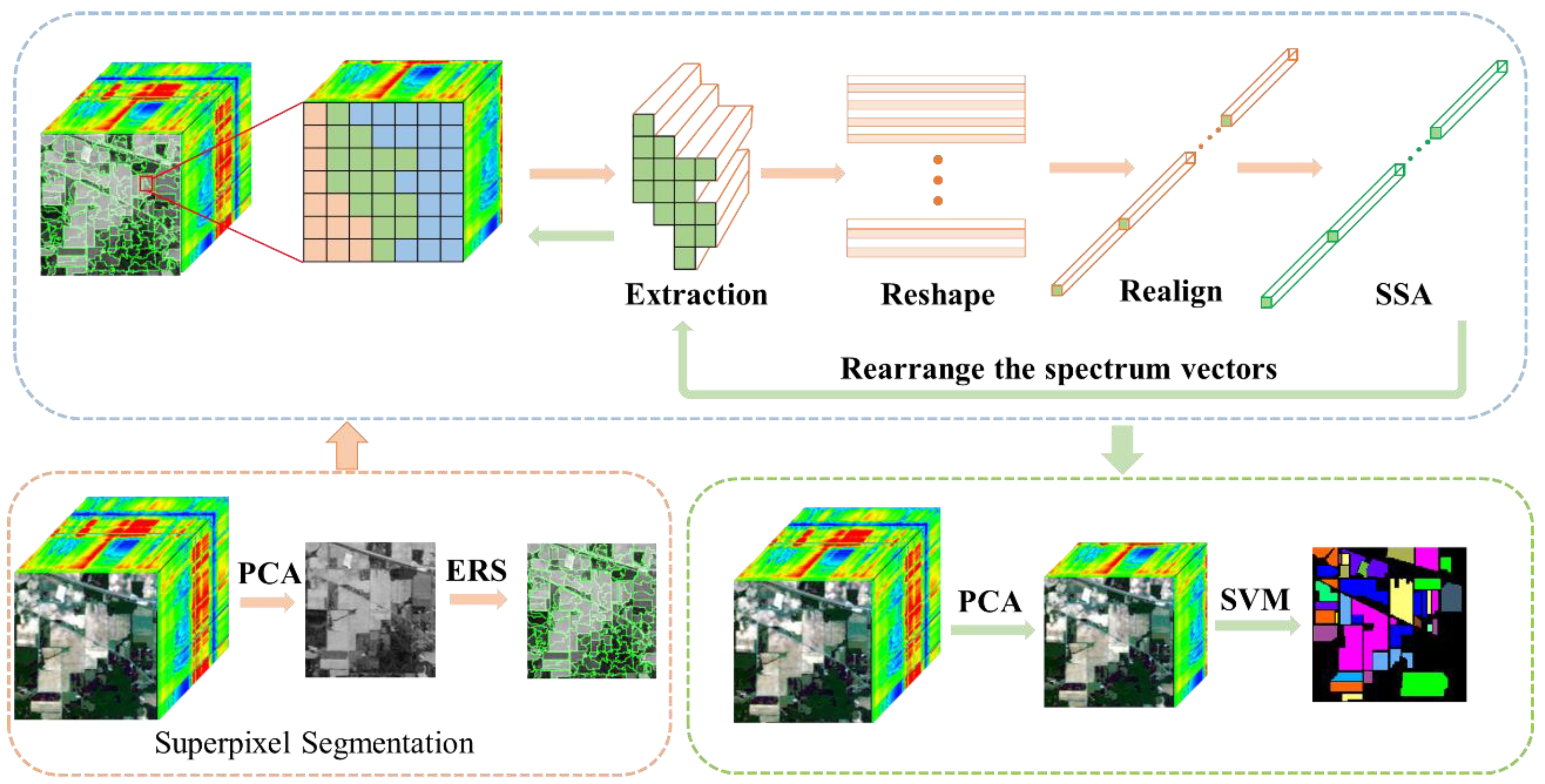
In this section, we mainly introduce the HSI classification method based on WSA-SSA. The method can be roughly divided into three steps: (1) region division according to the spatial information; (2) spatial–spectral features of HSI extraction based on WSA-SSA; and (3) classification. Figure 1 is a flow diagram of the proposed classification method. The following part describes the three steps in detail.
3.1. Region Division Based on Spatial Information
Segmentation of minor regions preserves locally valid information and boundary information of the image. Superpixel segmentation technology can divide pixels with similar characteristics into small areas. Using superpixel to describe image features reduces computational complexity and is generally used as a pre-processing step in image processing [40]. Among the many superpixel segmentation algorithms, the most widely used methods are entropy rate segmentation (ERS) [41] and simple linear iterative clustering (SLIC) [42]. The ERS preserves the boundary information of the image to the greatest extent but generates superpixels with irregular shapes. The shape of the superpixel obtained by the SLIC is more regular, but it partially destroys the boundary information and provides an inaccurate description of the contours. In the process of image preprocessing for HSI classification, the ERS algorithm is used to preprocess the HSI to retain the intact boundary information without affecting the classification results. To reduce the amount of computation, the PCA algorithm is used to reduce the dimension of HSI, the first principal component after dimensionality reduction is segmented by superpixel, and different labels are assigned to different superpixel regions, facilitating subsequent feature extraction and classification.
3.2. WSA-SSA
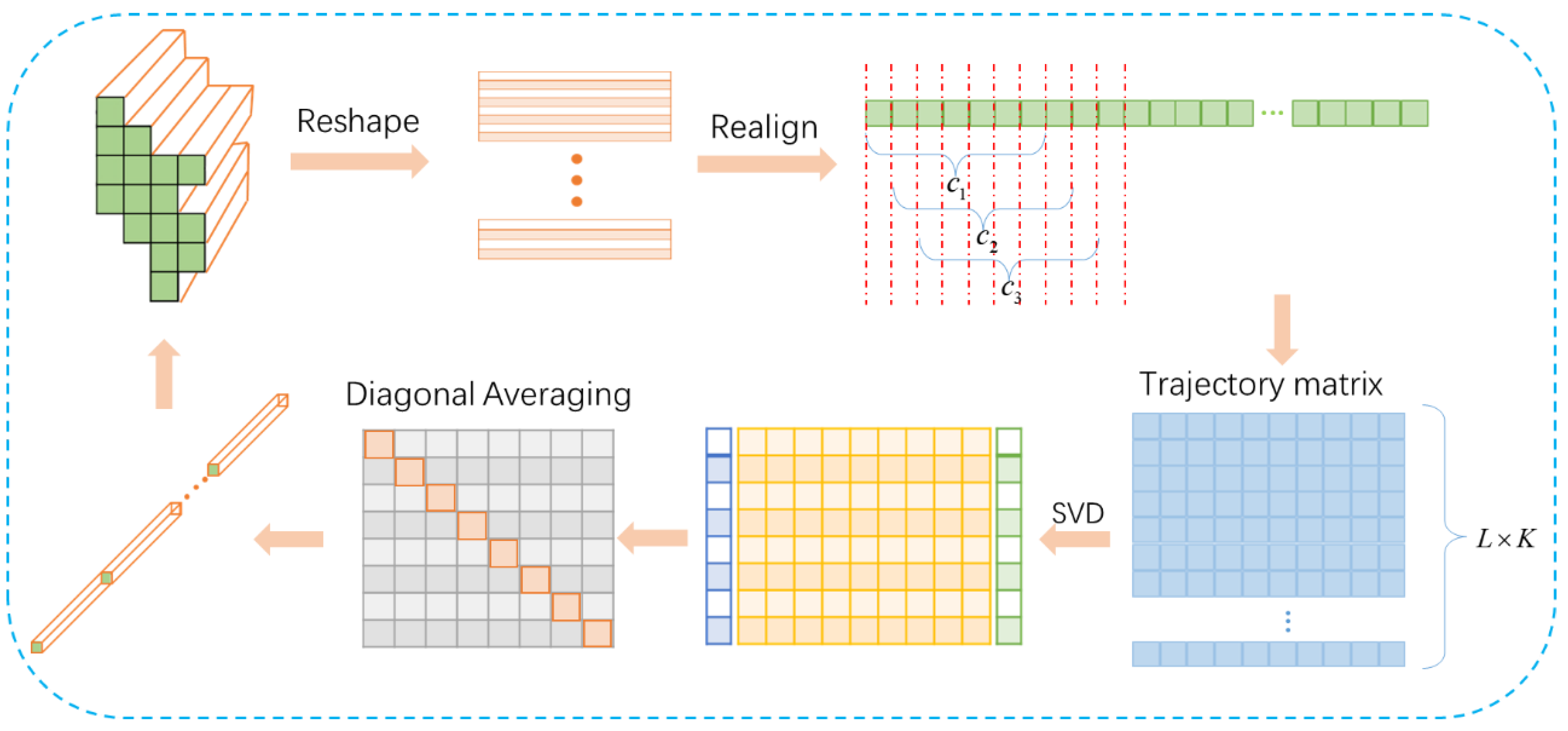
The ERS method is employed for superpixel segmentation of the first principal component of the Hyperspectral Image (HSI). This process involves partitioning the image into small, irregularly shaped regions based on the first principal component, assigning different labels to distinct regions, and ensuring that pixels within these irregularly shaped areas share similar characteristics. Features of the HSI are then extracted based on the positions of obtained superpixel labels. The proposed WSA-SSA algorithm in this paper identifies superpixel labels, determines their positions, and records their coordinate locations. The recorded coordinates, selected according to the labels, are located on the HSI, and subsequent calculations are performed only on the regions with the same label. The processed portions, chosen based on the labels, are illustrated in Figure 2.
A superpixel is defined as , consisting of pixel vectors denoted as , where is the position coordinate of the pixel in the superpixel and represents the spectral dimension. Since it is an irregularly shaped superpixel, the pixels in the superpixel are arranged into a one-dimensional spectral vector by the order of coordinate values, denoted as , where is the HSI spectral dimension. The spectral vector contains the local spatial information and spectral information of HSI. is defined as the one-dimensional signal . The appropriate window length is selected to arrange the signal with a lag to obtain the trajectory matrix, and the window size is equal to the number of extracted components. The matrix is the trajectory matrix of the one-dimensional signal, where and the column vector of the trajectory matrix is the lag vector.
Next, the SVD of the trajectory matrix is performed. Let , be the eigenvalues, , and is the matrix corresponding to the standard orthogonal vector of these eigenvalues. Let (note that in the actual sequence, there are usually ) and , in which case the SVD of the trajectory matrix can be written as
where is a primitive matrix of rank 1, and and are called the components of the empirical orthogonal function and trajectory matrix, respectively. The matrix is constructed as follows:
where represents the contribution of the eigenvalue to the matrix.
In order to separate the target signal components from the other signal components, the set of subscripts is divided into disjoint subsets such that , which corresponds to the synthesis matrix . After the combination, the trajectory matrix becomes
Transform each matrix in Equation (5) into a new length sequence , thus obtaining the decomposed sequence. Let be a matrix of with elements , , and . Let , , and . If , then ; otherwise, . Perform diagonal averaging using Equation (6) to transform the matrix N into a sequence .
The reconstructed feature sequence is separated into spectral vectors according to the number of pixels and spectral dimensions contained within the superpixel before reconstruction, and the separated spectral vectors are formed into a new superpixel with the same size as the superpixel before feature extraction according to the position coordinates recorded by . All the small regions are decomposed and reconstructed by the WSA-SSA to form an HSI local spatial–spectral feature image according to the label position of this superpixel, which contains HSI spectral information and local spatial information.
3.3. Classifier
Due to the high spectral dimensionality of HSI, it is still difficult to obtain a large number of training samples based on existing techniques, leading to the Hughes phenomenon in HSI. Due to the robustness of SVM to Hughes phenomenon [43], in the classification stage, SVM with a quintuple cross-validated Gaussian kernel is selected for the final implementation of classification.
4. Experiments and Analysis
To evaluate the extraction ability of the proposed method for the spatial–spectral specialization of HSIs, three basic HSI datasets—Indian Pines, Pavia University, and Salinas—are selected for experiments in this paper. This section presents the three basic datasets, experimental parameter settings, and comparative experimental results.
4.1. Data Set
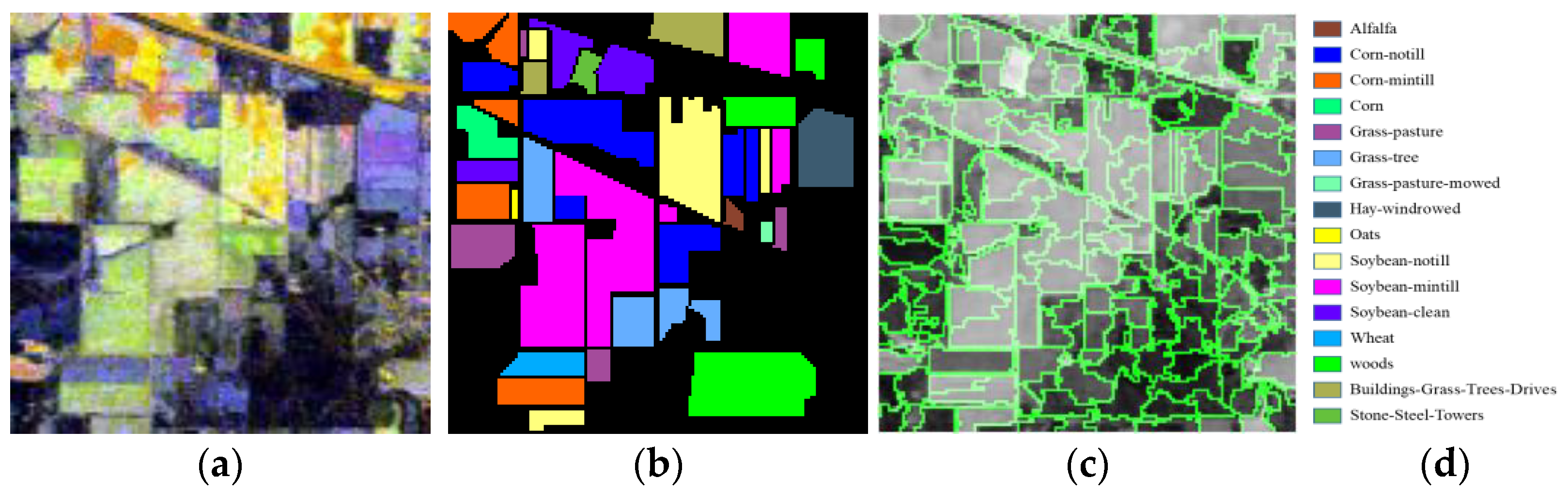
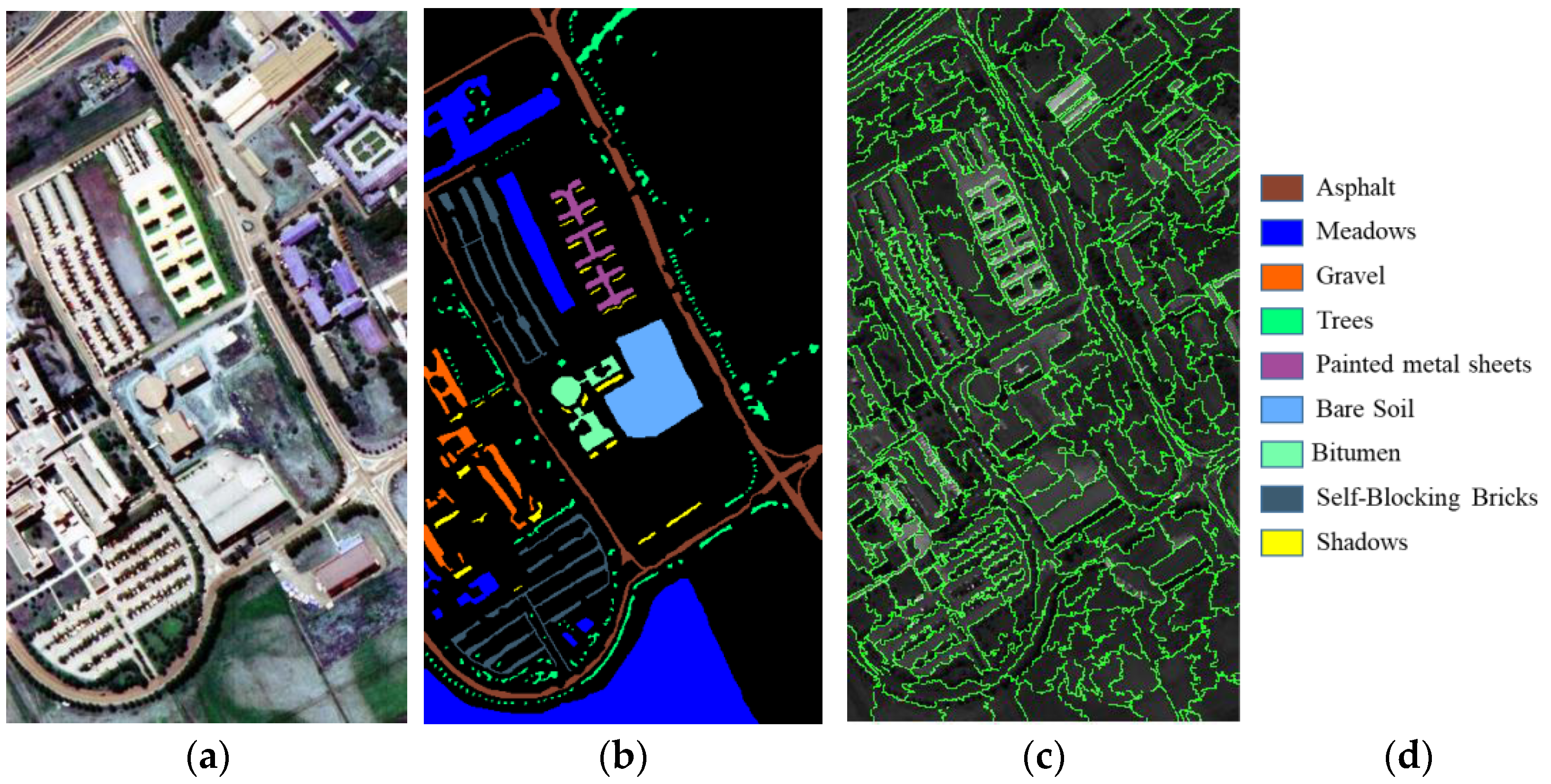
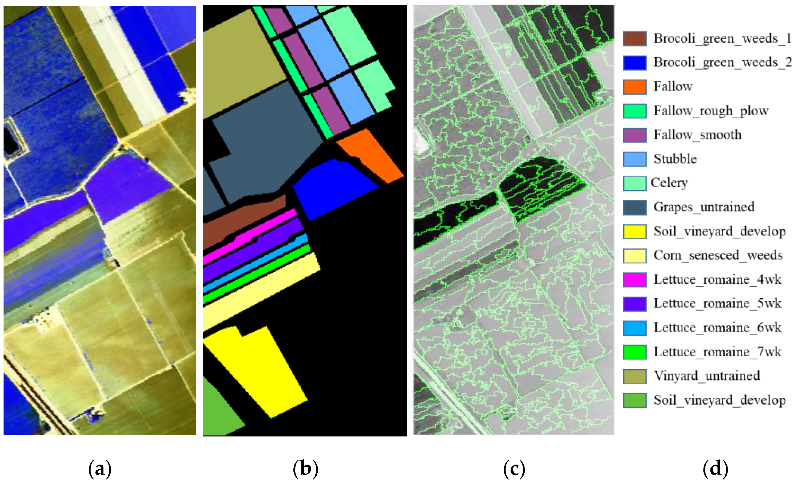
The three base datasets of Indian Pines, Pavia University, and Salinas were acquired by each mainstream sensor in different scenes with significant differences in the number of bands, spectral resolution, and image size [44]. The detailed parameters are shown in Table 1, and the pseudo-color, Ground truth, and superpixel segmentation maps of the three datasets are shown in Figure 3, Figure 4 and Figure 5.
4.2. Parameter Sensitivity Analysis
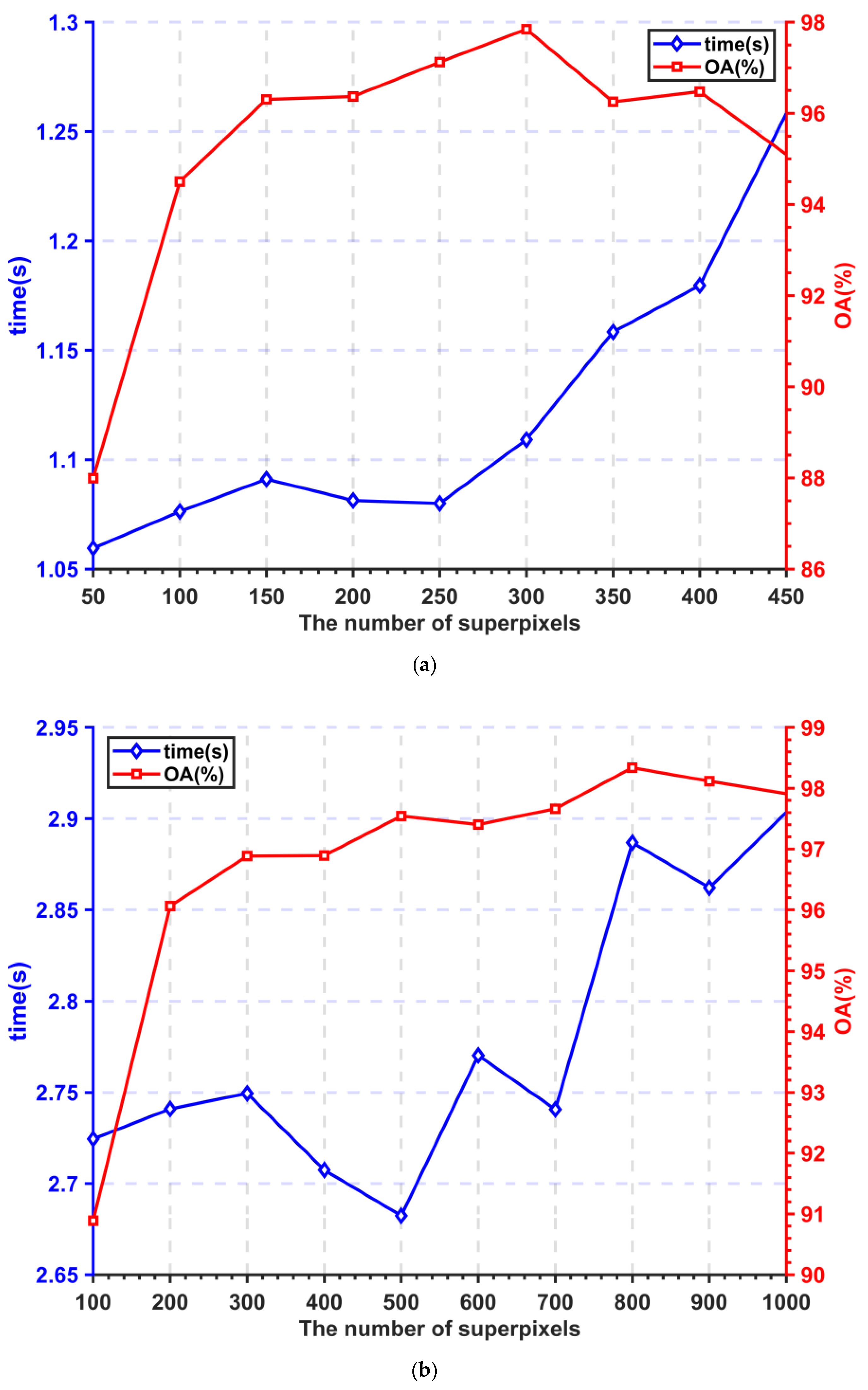
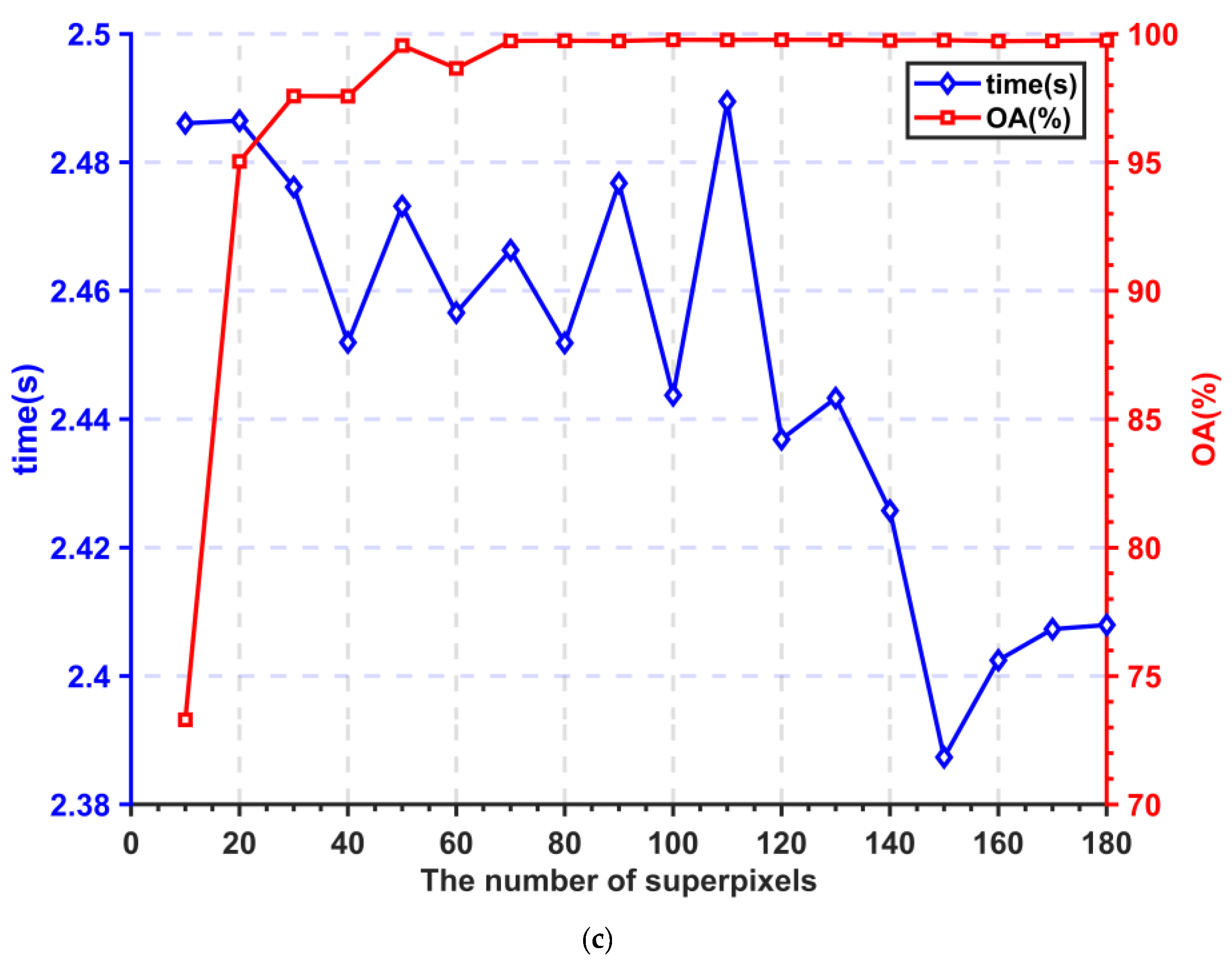
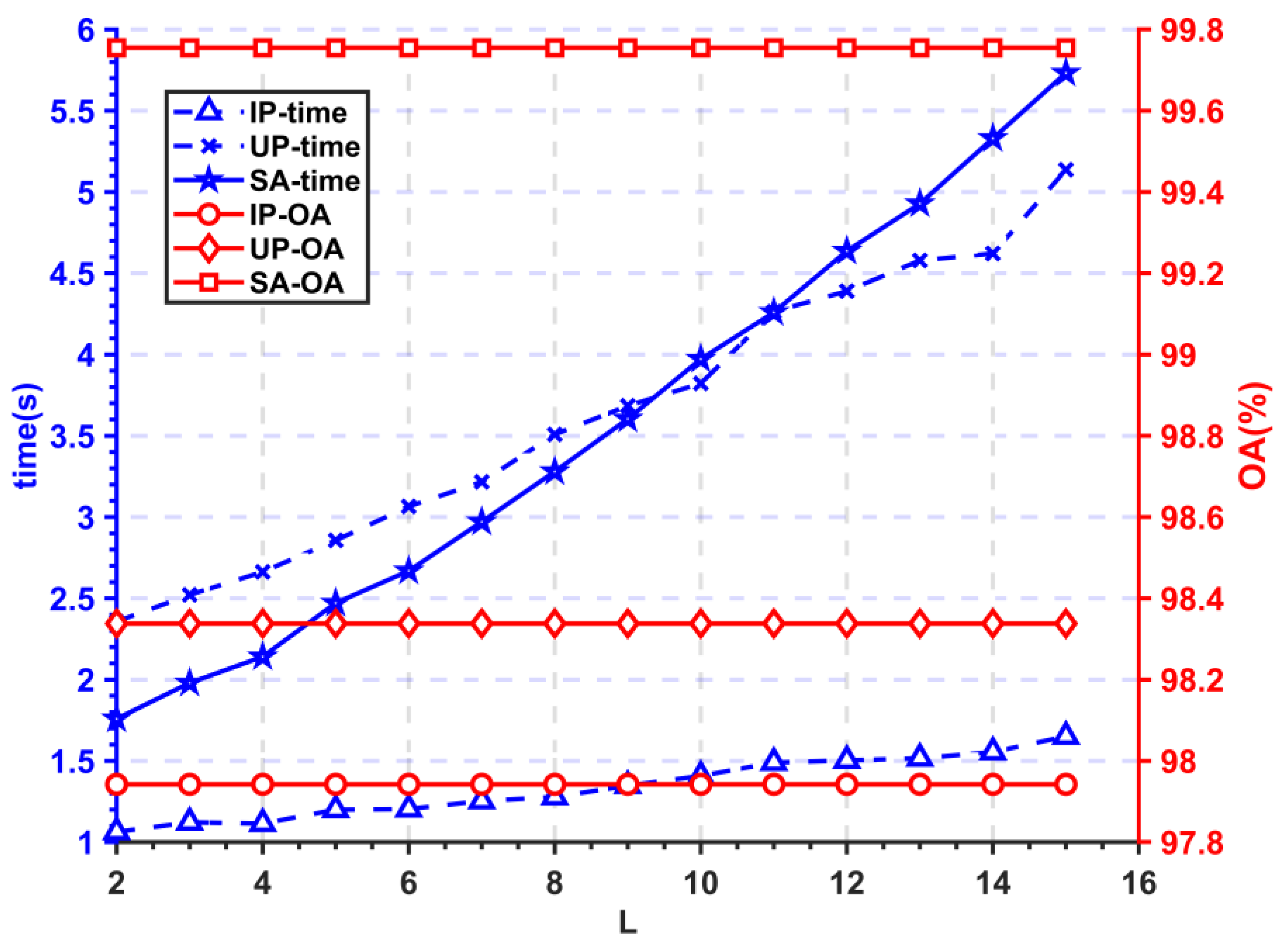
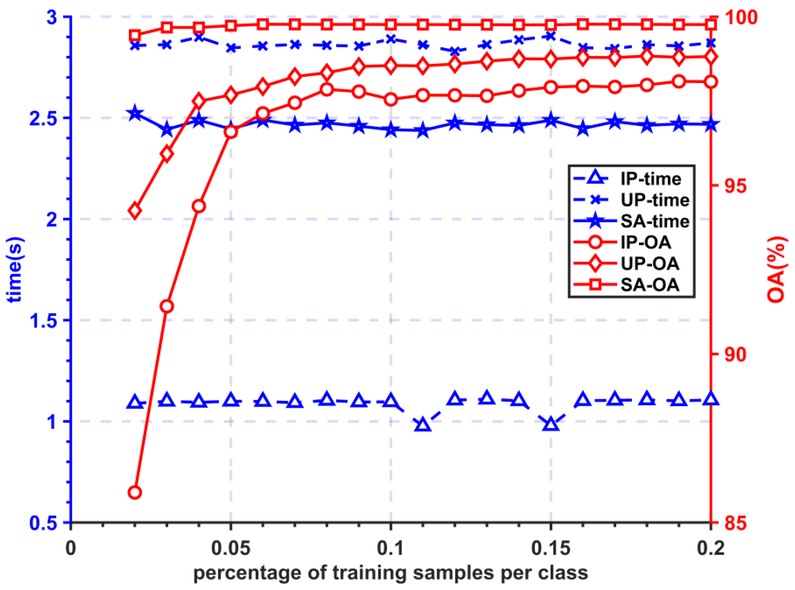
Two main parameters of WSA-SSA affect the capability of extracting spectral–spatial features, running time, and classification accuracy. To be able to extract rich spatial–spectral features, the window size of WSA-SSA, which is the number of pixels contained in the segmented superpixel, is an important parameter that directly affects the classification accuracy and the running time. The proposed method is improved based on SSA to extract spectral information and local spatial information simultaneously, and its EVG value is fixed to 1. The scale L of SSA is also an important parameter that determines the reconstruction accuracy of the spectral–spatial features of the lagging vector in the trajectory matrix. If the scale is too large, which means the embedding window is too large, it is easy to construct a larger trajectory matrix and increase the computational effort. The scale should not be too small, because the smoothing ability of the data decreases and the noise-removal ability becomes weaker. The effects of these two parameters on the classification accuracy of the HSI of the three datasets are shown in Figure 6 and Figure 7.
The value of the parameter determines the size of the superpixel, the superpixel area determines the window size of the proposed method, and the arrangement of pixels in the superpixel determines the window shape of the proposed method. The experimental results show that the larger the number of superpixels in a certain range, the higher the classification accuracy obtained. This is because the smaller the segmented superpixel is, the greater the possibility that neighboring pixels belong to the same class of features, and the higher their pixel similarity. By using WSA-SSA to reconstruct the pixels in the area, each pixel contains both its spectral information and the information of pixels with high similarity in the domain, achieving the purpose of obtaining both spectral and local spatial information. Meanwhile, a larger number of superpixels increases the processing times of WSA-SSA but decreases the processing time of single WSA-SSA. The smaller the number of superpixels, the larger the divided area is, the greater the possibility of containing different classes of features in the same area, and the more easily are the reconstructed hyperspectral pixels in its area mixed with information that do not belong to the same class of pixels, which reduces the classification accuracy. At the same time, a smaller number of superpixels reduces the amount of WSA-SSA processing but increases the running time of one WSA-SSA.
The traditional SSA is mostly used to process time series, which only retains the overall trend of the data and easily ignores the higher frequency peaks in the series, and is applied to the processing of HSI spectral vectors, which easily loses the higher frequency peaks in spectral vectors. The experimental results of the effect of scale L of WSA-SSA on the classification accuracy and running time are shown in Figure 7. The variation of scale L within a certain range has a small effect on the classification accuracy and a large effect on the running time. Since the larger the scale L is, and the larger the dimension of the trajectory matrix it constructs, the higher its decomposition is. The larger dimensionality of the trajectory matrix increases the computation volume and prolongs the computation time. The higher the degree of decomposition of the sequence data, the more complete the retention of the components called high frequencies in the spectral vector, but too high a degree of decomposition reduces the ability to eliminate noise. The proposed method rearranges the spectral vectors with high similarity in the superpixel to form the approximate periodic sequence spectral data, which better exploit the processing capability of the SSA for spectral vectors.
4.3. Comparison Experiments
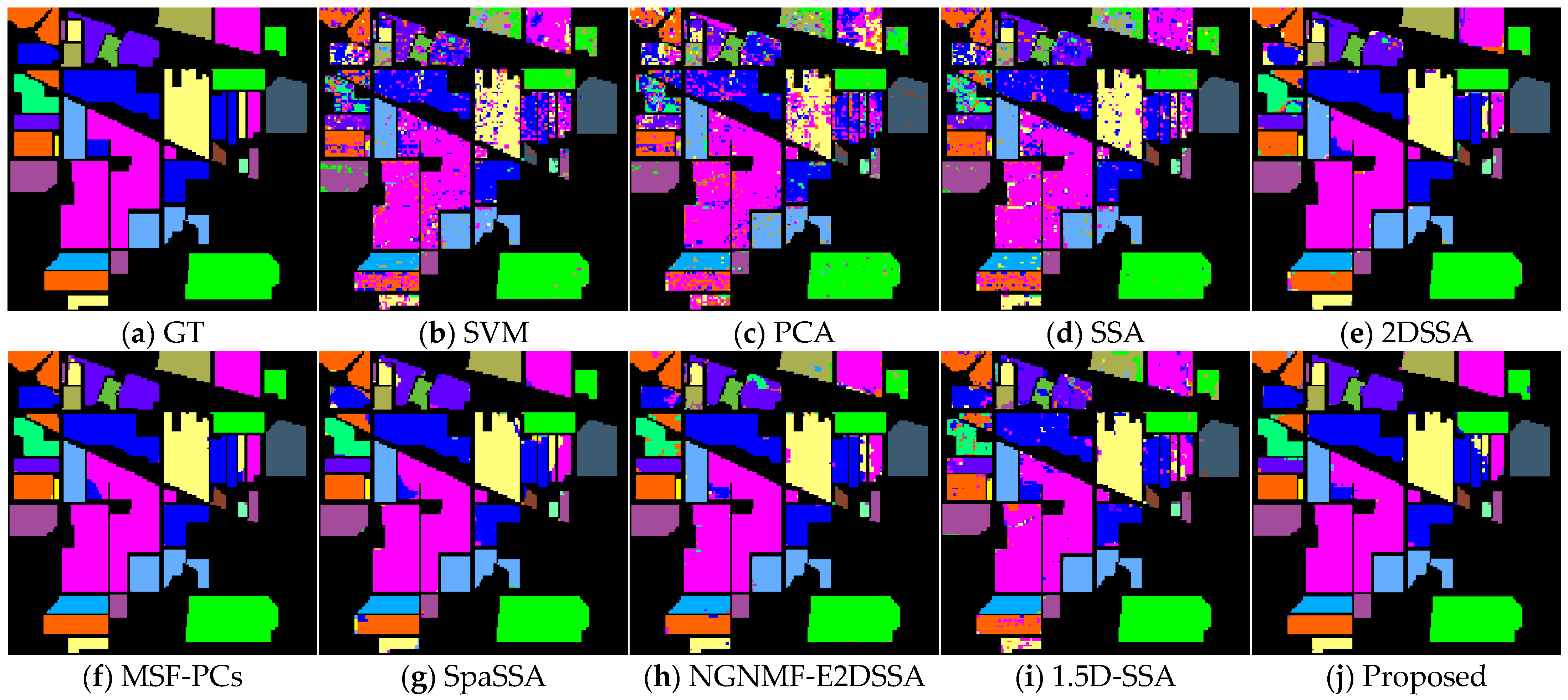
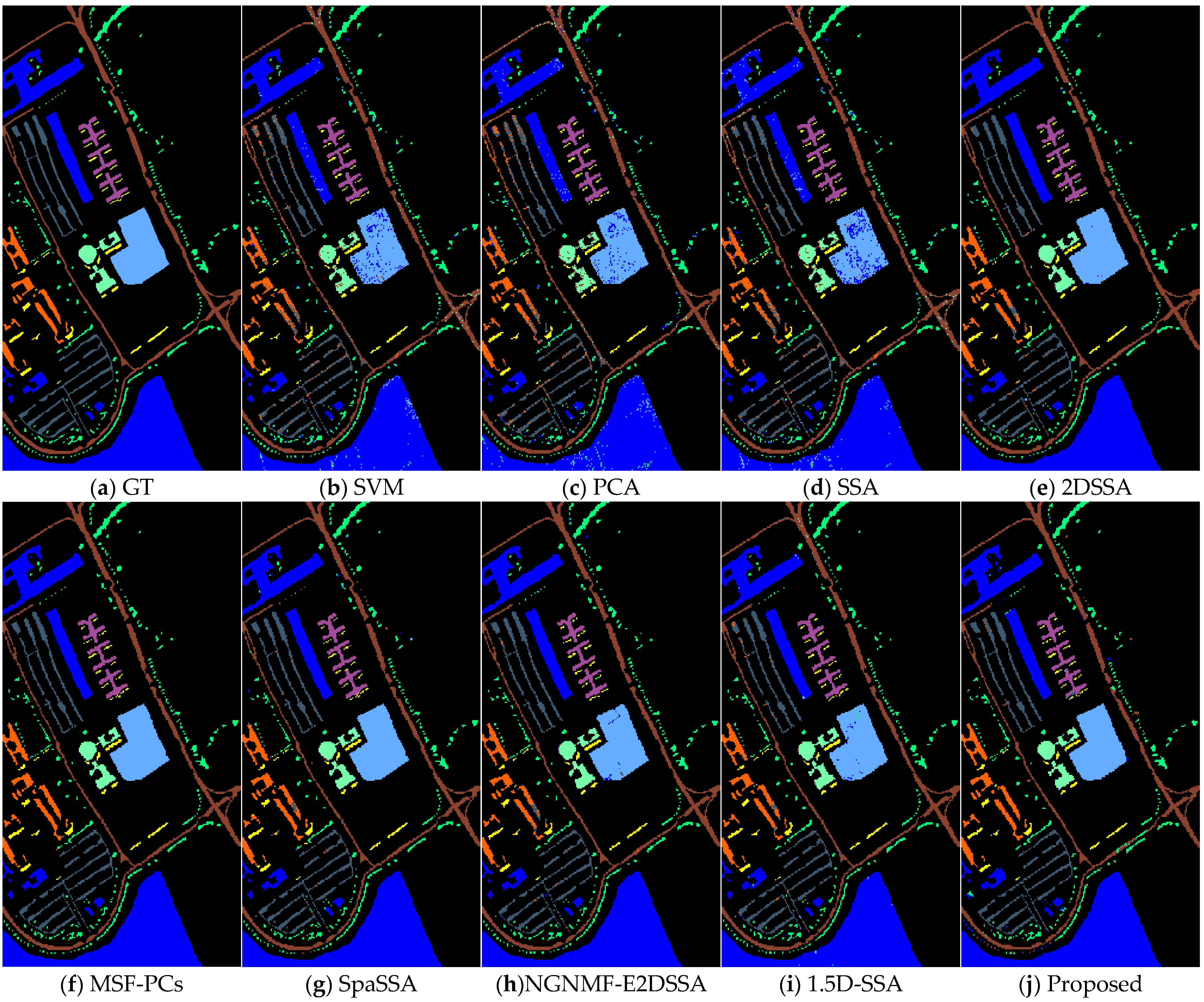
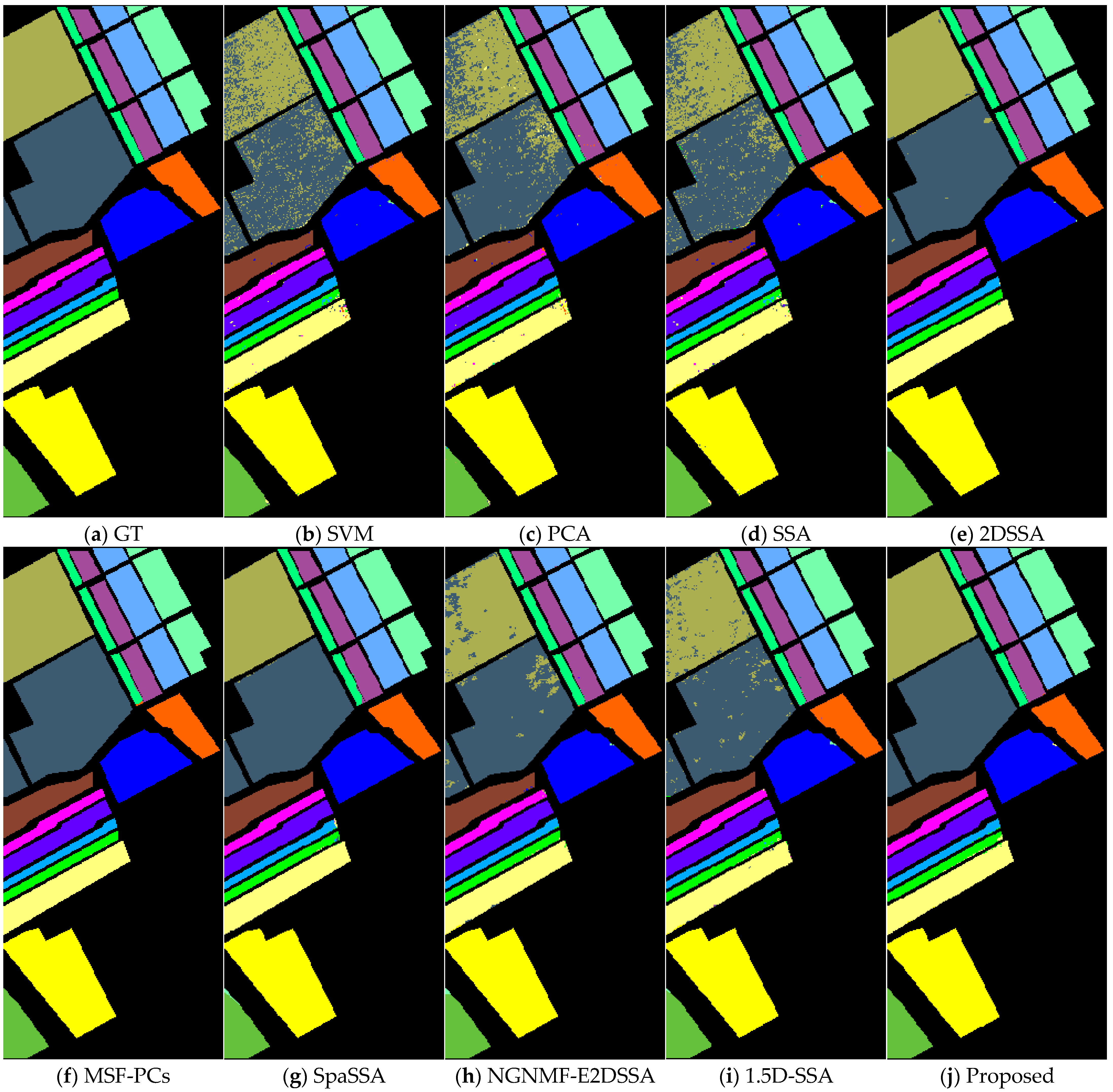
In this section, the proposed method is experimented on three widely used datasets—Indian Pines, Pavia University, and Salinas—and the performance is compared with some HSI classification methods. To verify the effectiveness of the proposed method, 8% of the labeled samples are randomly selected in each feature type as the training set, and the remaining 92% of the labeled samples are used as the test set. The main methods compared are SVM for the classification of raw data; traditional 1DSSA and 2DSSA combined with SVM, respectively; PCA combined with SVM; and classification methods that have performed better in the last two years. In the experiments, the classifier is selected for the classification method of SVM. The parameters of the Gaussian kernel are uniformly set to , . For the PCA combined with the SVM classification method, the same as the proposed method is chosen for the first 30 components of PCA for classification experiments. For the feature extraction stage, the scale of SSA is and the window size of 2DSSA is . The optimal parameters from their papers were used for MSF-PCs (2020), SpaSSA (2022), NGNMF-E2DSSA (2022) [45], and 1.5D-SSA (2020). To avoid the chance of experimental results, all experiments were performed 10 times with the same equipment, and the results of all numerical indicators are the average of 10 experiments. The effect plots of all the above classification methods are shown in Figure 8, Figure 9 and Figure 10.
From the classification results, the proposed method achieves very good results on all three datasets. Compared with the SVM, PCA followed by the classification method, and SSA and 2DSSA for feature extraction followed by classification, there is a significant improvement, indicating that the proposed method makes full use of the local spatial and spectral information of HSI to achieve good classification results more easily than using spatial or spectral information alone. Compared with the SpaSSA, NGNMF-E2DSSA, and 1.5D-SSA methods, the proposed method shows obvious advantages in classifying adjacent features. This is because the first three methods use a fixed rectangular window for feature extraction of HSI, followed by SVM for classification. When a fixed shape window is used to traverse each pixel for feature extraction, if the window contains different kinds of feature pixels, it will lead to poor reconstruction accuracy, thus affecting the classification results. The proposed WSA-SSA algorithm, without a fixed shape window, can reconstruct every pixel in the region on an arbitrarily shaped superpixel, demonstrating good edge-retention capability.
To compare the classification performance of each algorithm more objectively, this paper uses four metrics: overall accuracy (OA), average accuracy (AA), and Kappa coefficient (Kappa) time consumed by classification (time) to measure the classification performance of the algorithms. OA refers to the number of correctly classified samples in the total test samples; AA represents the average of classification accuracy; Kappa provides information about the ground truth and mutual information about the strong agreement between the graph and the classification graph. The numerical results of the experiments on the three datasets are shown in Table 2, Table 3 and Table 4.
As can be seen from Table 2, on the Indian Pines dataset, the proposed method has a significant improvement effect in extracting discriminative classification features compared with the traditional SSA algorithm and the 2DSSA algorithm, which extends to extract spatial information, and the overall classification accuracy, average classification accuracy, and Kappa coefficient are higher than the SVM algorithm by about 20% and higher than the traditional SSA algorithm by 14%. Above all, the proposed method achieved excessive smoothing of the input spectral vector by the traditional SSA. Only the trend of the spectral vector change can be retained, resulting in a lower classification effect. The proposed method is slightly higher than the other algorithms except for MSF-PCs in three measures of classification accuracy. In particular, it performs well in small-sample feature classification, such as the classification of Alfalfa, which has only 48 samples and 3–4 randomly selected samples in the training set, and the overall classification accuracy reaches 97.62%, which is much higher than that of the other methods in the table, indicating that the proposed method has excellent performance in small-sample classification tasks. In addition, the proposed method has a significant advantage in terms of running time. The NGNMF-E2DSSA algorithm, MSF-PCs algorithm, and 1.5D-SSA algorithm take more than 10 s to complete the classification on the Indian Pines dataset, and the SpaSSA algorithm takes 24 s, while the proposed method takes only 1.13 s to complete the classification with high accuracy. Since the WSA-SSA does not traverse every pixel operation with a fixed rectangular window, it directly deals with irregularly shaped superpixels, extracts spectral information and spatial structure information in the region, and reconstructs the superpixels, which significantly reduces the computational effort and shortens the running time.
It can be visualized from Table 3 and Table 4 that the overall classification accuracy of the window shape adaptive SSA algorithm can reach 98.34% and 99.77% on the Pavia University dataset and Salinas dataset; the average classification accuracy reaches 97.79% and 99.46%, respectively; and the corresponding Kappa coefficients are high, showing good performance. An accuracy of 100% can be achieved in the classification of some categories of features. Similarly, it can be seen in Table 3 and Table 4 that the proposed method can achieve more than 99.5% accuracy in the classification of small sample feature categories. In addition, due to the larger spatial dimensions of both the Pavia University dataset and the Salinas dataset over the Indian Pines dataset, the computational effort of each algorithm in the table increases and the running time becomes significantly longer. The running time of the NGNMF-E2DSSA algorithm, SpaSSA algorithm, and MSF-PCs algorithm on the Pavia University data set takes more than 100 s, while the proposed method in this paper takes only 2.84 s. On the Salinas dataset, the WSA-SSA also takes only 2.71 s to finish the classification, which is far ahead of the other algorithms. The advantage of WSA-SSA in reducing the computational effort is more prominent in large-size images, where it can achieve fast classification results. The proposed method has potential applications in other fields, such as holographic displays [46,47], image compression [48,49], optical imaging [50,51,52], etc.
5. Conclusions
This paper analyzes the characteristics of hyperspectral images as a three-dimensional data cube containing millions of pixels; the volume of data processing is substantial, leading to an extended processing duration. Introducing the WSA-SSA algorithm, it is crafted to simultaneously extract spectral features and local spatial features. The algorithm dynamically adjusts to diverse window shapes, a pivotal capability for alleviating misclassification at the boundaries of different species, particularly when dealing with irregular shapes within feature regions. This results in better and more accurate classification of boundary pixels. Importantly, the algorithm does not employ a fixed window for iterating over each pixel, reducing computational complexity. Moreover, a classification algorithm based on WSA-SSA is introduced. It partitions hyperspectral images based on spatial information; employs the WSA-SSA algorithm for spectral and spatial feature extraction; and, finally, combines SVM for feature classification. This approach achieves high-precision classification on three benchmark datasets while significantly reducing the classification time. Although WSA-SSA demonstrates excellent performance on these datasets, it focuses solely on spectral and local spatial information during feature extraction, neglecting global spatial information. In future work, the 2DSSA algorithm could be introduced to consider global spatial information and enhance classification accuracy.
Author Contributions
Conceptualization, X.B. and G.L.; methodology, X.B.; software, X.B. and B.Q.; validation, X.B., B.Q. and J.L.; formal analysis, J.L.; data curation, X.B. and L.J.; writing—original draft preparation, X.B.; writing—review and editing, G.L., B.Q. and J.L; project management, G.L. and J.L. All authors have read and agreed to the published version of the manuscript.
Funding
This research received no external funding.
Data Availability Statement
Data are contained within the article.
Conflicts of Interest
The authors declare no conflict of interest.
References
- AVHYAS: A Free and Open Source QGIS Plugin for Advanced Hyperspectral Image Analysis. In Proceedings of the 2021 International Conference on Emerging Techniques in Computational Intelligence (ICETCI), Hyderabad, India, 25–27 August 2021; pp. 71–76.
- Song, X.; Sunil, A.; Kai, M.T.; Zhen, L.; Bin, H. Spectral-Spatial Anomaly Detection of Hyperspectral Data Based on Improved Isolation Forest. IEEE Trans. Geosci. Remote Sens. 2022, 60, 1–16. [Google Scholar] [CrossRef]
- Li, H. An Overview on Remote Sensing Image Classification Methods with a Focus on Support Vector Machine. In Proceedings of the 2021 International Conference on Signal Processing and Machine Learning (CONF-SPML), Stanford, CA, USA, 14 November 2021; pp. 50–56. [Google Scholar]
- Liu, H.; Li, W.; Xia, X.-G.; Zhang, M.; Gao, C.-Z.; Tao, R. Central Attention Network for Hyperspectral Imagery Classification. IEEE Trans. Neural Netw. Learn. Syst. 2022, 34, 8989–9003. [Google Scholar] [CrossRef] [PubMed]
- Rasti, B.; Hong, D.; Hang, R.; Ghamisi, P.; Kang, X.; Chanussot, J.; Benediktsson, J.A. Feature extraction for hyperspectral imagery: The evolution from shallow to deep: Overview and toolbox. IEEE Geosci. Remote Sens. Mag. 2020, 8, 60–88. [Google Scholar] [CrossRef]
- Peng, J.; Sun, W.; Du, Q. Self-paced joint sparse representation for the classification of hyperspectral images. IEEE Trans. Geosci. Remote Sens. 2018, 57, 1183–1194. [Google Scholar] [CrossRef]
- Su, H.; Yong, B.; Du, P.; Liu, H.; Chen, C.; Liu, K. Dynamic classifier selection using spectral-spatial information for hyperspectral image classification. J. Appl. Remote Sens. 2014, 8, 085095. [Google Scholar] [CrossRef]
- Tyo, J.S.; Konsolakis, A.; Diersen, D.I.; Olsen, R.C. Principal-components-based display strategy for spectral imagery. IEEE Trans. Geosci. Remote Sens. 2003, 41, 708–718. [Google Scholar] [CrossRef]
- Chiu, S.-H.; Lu, C.-P.; Wu, D.-C.; Wen, C.-Y. A histogram based data-reducing algorithm for the fixed-point independent component analysis. Pattern Recognit. Lett. 2008, 29, 370–376. [Google Scholar] [CrossRef]
- Chen, M.; Wang, Q.; Li, X. Discriminant Analysis with Graph Learning for Hyperspectral Image Classification. Remote. Sens. 2018, 10, 836. [Google Scholar] [CrossRef]
- Guan, L.; Xie, W.; Pei, J. Segmented minimum noise fraction transformation for efficient feature extraction of hyperspectral images. BPRA Int. Conf. Pattern Recognit. 2015, 48, 3216–3226. [Google Scholar]
- Bachmann, C.M.; Ainsworth, T.L.; Fusina, R.A. Exploiting manifold geometry in hyperspectral imagery. IEEE Trans. Geosci. Remote Sens. 2005, 43, 441–454. [Google Scholar] [CrossRef]
- Li, B.; Li, Y.-R.; Zhang, X.-L. A survey on Laplacian eigenmaps based manifold learning methods. Neurocomputing 2019, 335, 336–351. [Google Scholar] [CrossRef]
- Roweis, S.T.; Saul, L.K. Nonlinear Dimensionality Reduction by Locally Linear Embedding. Science 2000, 290, 2323–2326. [Google Scholar] [CrossRef] [PubMed]
- Zabalza, J.; Ren, J.; Wang, Z.; Marshall, S.; Wang, J. Singular Spectrum Analysis for Effective Feature Extraction in Hyperspectral Imaging. IEEE Geosci. Remote Sens. Lett. 2014, 11, 1886–1890. [Google Scholar] [CrossRef]
- Benediktsson, J.A.; Pesaresi, M.; Arnason, K. Classification and feature extraction for remote sensing images from urban areas based on morphological transformations. IEEE Trans. Geosci. Remote Sens. 2003, 41, 1940–1949. [Google Scholar] [CrossRef]
- Benediktsson, J.A.; Palmason, J.A.; Sveinsson, J.R. Classification of hyperspectral data from urban areas based on extended morphological profiles. IEEE Trans. Geosci. Remote Sens. 2005, 43, 480–491. [Google Scholar] [CrossRef]
- Mauro, D.M.; Jon, A.B.; Björn, W.; Lorenzo, B. Morphological Attribute Profiles for the Analysis of Very High Resolution Images. IEEE Trans. Geosci. Remote Sens. 2010, 48, 3747–3762. [Google Scholar]
- Mauro, D.M.; Alberto, V.; Jon, A.B.; Jocelyn, C.; Lorenzo, B. Classification of Hyperspectral Images by Using Extended Morphological Attribute Profiles and Independent Component Analysis. IEEE Geosci. Remote Sens. Lett. 2011, 8, 542–546. [Google Scholar]
- Welch, R.M.; Sengupta, S.K.; Chen, D.W. Cloud field classification based upon high spatial resolution textural features: 1. Gray level co-occurrence matrix approach. J. Geophys. Res. 1988, 93, 12663–12681. [Google Scholar] [CrossRef]
- Kim, S.-D.; Udpa, S. Texture classification using rotated wavelet filters. IEEE Trans. Syst. Man Cybern. Syst. 2000, 30, 847–852. [Google Scholar]
- Jia, S.; Lin, Z.; Deng, B.; Zhu, J.; Li, Q. Cascade Superpixel Regularized Gabor Feature Fusion for Hyperspectral Image Classification. IEEE Trans. Neural Netw. 2020, 31, 1638–1652. [Google Scholar] [CrossRef]
- Yan, S.; Xu, D.; Zhang, B.; Zhang, H.J.; Yang, Q.; Lin, S. Graph Embedding and Extensions: A General Framework for Dimensionality Reduction. IEEE Trans. Pattern Anal. Mach. Intell. 2007, 29, 40–51. [Google Scholar] [CrossRef] [PubMed]
- Zabalza, J.; Ren, J.; Zheng, J.; Han, J.; Zhao, H.; Li, S.; Marshall, S. Novel Two-Dimensional Singular Spectrum Analysis for Effective Feature Extraction and Data Classification in Hyperspectral Imaging. IEEE Trans. Geosci. Remote Sens. 2015, 53, 4418–4433. [Google Scholar] [CrossRef]
- Hang, F.; Sun, G.; Zabalza, J.; Zhang, A.; Ren, J.; Jia, X. A Novel Spectral-Spatial Singular Spectrum Analysis Technique for Near Real-Time In Situ Feature Extraction in Hyperspectral Imaging. IEEE J. Sel. Top. Appl. Earth Obs. Remote Sens. 2020, 13, 2214–2225. [Google Scholar]
- Hang, F.; Sun, G.; Ren, J.; Zhang, A.; Jia, X. Fusion of PCA and Segmented-PCA Domain Multiscale 2-D-SSA for Effective Spectral-Spatial Feature Extraction and Data Classification in Hyperspectral Imagery. IEEE Trans. Geosci. Remote Sens. 2022, 60, 1–14. [Google Scholar]
- Sun, G.; Hang, F.; Ren, J.; Zhang, A.; Zabalza, J.; Jia, X.; Zhao, H. SpaSSA: Superpixelwise Adaptive SSA for Unsupervised Spatial–Spectral Feature Extraction in Hyperspectral Image. IEEE Trans. Cybern. 2022, 52, 6158–6169. [Google Scholar] [CrossRef] [PubMed]
- Swalpa, K.R.; Gopal, K.; Shiv, R.D.; Bidyut, B.C. HybridSN: Exploring 3-D-2-D CNN Feature Hierarchy for Hyperspectral Image Classification. Comput. Res. Repos. 2020, 17, 277–281. [Google Scholar]
- Hang, R.; Li, Z.; Liu, Q.; Ghamisi, P.; Bhattacharyya, S.S. Hyperspectral Image Classification with Attention-Aided CNNs. IEEE Trans. Geosci. Remote Sens. 2021, 59, 2281–2293. [Google Scholar] [CrossRef]
- Mei, X.; Pan, E.; Ma, Y.; Dai, X.; Huang, J.; Fan, F.; Du, Q.; Zheng, H.; Ma, J. Spectral-Spatial Attention Networks for Hyperspectral Image Classification. Remote Sens. 2019, 11, 963. [Google Scholar] [CrossRef]
- Lee, H.; Kwon, H. Going Deeper with Contextual CNN for Hyperspectral Image Classification. IEEE Trans. Image Process. 2017, 26, 4843–4855. [Google Scholar] [CrossRef]
- Hong, D.; Han, Z.; Yao, J.; Gao, L.; Zhang, B.; Plaza, A.; Chanussot, J. SpectralFormer: Rethinking Hyperspectral Image Classification with Transformers. IEEE Trans. Geosci. Remote Sens. 2022, 60, 1–15. [Google Scholar] [CrossRef]
- Vautard, R.; Yiou, P.; Ghil, M. Singular-spectrum analysis: A toolkit for short, noisy chaotic signals. Phys. D Nonlinear Phenom. 1992, 58, 95–126. [Google Scholar] [CrossRef]
- Zhong, Z.; Li, Y.; Ma, L.; Li, J.; Zheng, W.S. Spectral–spatial transformer network for hyperspectral image classification: A factorized architecture search framework. IEEE Trans. Geosci. Remote Sens. 2021, 60, 1–15. [Google Scholar] [CrossRef]
- Danilov, D.; Zhiglyavskii, A. Principal Components of Time Series: The ‘Caterpillar’ Method; St. Petersburg University: Saint Petersburg, Russia, 1997; Available online: http://www.gistatgroup.com/cat/books.html (accessed on 1 October 2022). (In Russian)
- Golyandina, N.E.; Usevich, K.D. 2D-extension of Singular Spectrum Analysis: Algorithm and elements of theory. In Matrix Methods: Theory, Algorithms and Applications: Dedicated to the Memory of Gene Golub; World Scientific: Singapore, 2010; pp. 449–473. [Google Scholar]
- Rodríguez-Aragón, L.J.; Zhigljavsky, A. Singular spectrum analysis for image processing. Stat. Its Interface 2010, 3, 419–426. [Google Scholar] [CrossRef]
- Ren, X.; Malik, J. Learning a classification model for segmentation. In Proceedings of the IEEE International Conference on Computer Vision, Nice, France, 13–16 October 2003; Volume 1, pp. 10–17. [Google Scholar]
- Liu, M.-Y.; Tuzel, O.; Ramalingam, S.; Chellappa, R. Entropy rate superpixel segmentation. Comput. Vis. Pattern Recognit. 2011, 2011, 2097–2104. [Google Scholar]
- Luo, F.; Zhang, L.; Zhou, X.; Guo, T.; Cheng, Y.; Yin, T. Sparse-Adaptive Hypergraph Discriminant Analysis for Hyperspectral Image Classification. IEEE Geosci. Remote Sens. Lett. 2020, 17, 1082–1086. [Google Scholar] [CrossRef]
- Archibald, R.; Fann, G. Feature Selection and Classification of Hyperspectral Images with Support Vector Machines. IEEE Geosci. Remote Sens. Lett. 2007, 4, 674–677. [Google Scholar] [CrossRef]
- Hyperspectral Data Set [OL]. Available online: http://www.ehu.eus/ccwintco/index.php?title=Hyperspectral_Remote_Sensing_Scenes (accessed on 1 October 2022).
- Fu, H.; Zhang, A.; Sun, G.; Ren, J.; Jia, X.; Pan, Z.; Ma, H. A Novel Band Selection and Spatial Noise Reduction Method for Hyperspectral Image Classification. IEEE Trans. Geosci. Remote Sens. 2022, 60, 5535713. [Google Scholar] [CrossRef]
- Zhao, X.; Liu, K.; Gao, K.; Li, W. Hyperspectral Time-Series Target Detection Based on Spectral Perception and Spatial–Temporal Tensor Decomposition. IEEE Trans. Geosci. Remote Sens. 2023, 61, 5520812. [Google Scholar] [CrossRef]
- Zhao, X.; Li, W.; Zhao, C.; Tao, R. Hyperspectral Target Detection Based on Weighted Cauchy Distance Graph and Local Adaptive Collaborative Representation. IEEE Trans. Geosci. Remote Sens. 2022, 60, 5527313. [Google Scholar] [CrossRef]
- Li, J.; Smithwick, Q.; Chu, D. Holobricks: Modular coarse integral holographic displays. Light Sci. Appl. 2022, 11, 57. [Google Scholar] [CrossRef]
- Li, J.; Smithwick, Q.; Chu, D. Bandwidth utilization improvement methods of Coarse Integral Holographic video displays. In Imaging and Applied Optics 2018 (3D, AO, AIO, COSI, DH, IS, LACSEA, LS&C, MATH, pcAOP), OSA Technical Digest; Optica Publishing Group: Washington, DC, USA, 2018; Paper DTh3D.6. [Google Scholar]
- Li, J.; Liu, Z. Multispectral transforms using convolution neural networks for remote sensing multispectral image compression. Remote Sens. 2019, 11, 759. [Google Scholar] [CrossRef]
- Li, J.; Liu, Z. Efficient compression algorithm using learning networks for remote sensing images. Appl. Soft Comput. 2021, 100, 106987. [Google Scholar] [CrossRef]
- Tehseen, R.; Ali, A.; Mane, M.; Ge, W.; Li, Y.; Zhang, Z.; Xu, J. Enhanced imaging through turbid water based on quadrature lock-in discrimination and retinex aided by adaptive gamma function for illumination correction. Chin. Opt. Lett. 2023, 21, 101102. [Google Scholar] [CrossRef]
- Park, Y.S.; Hong, J.; Choi, J. X-ray volumetric quantitative phase imaging by Foucault differential filtering with linear scanning. Chin. Opt. Lett. 2023, 21, 013401. [Google Scholar] [CrossRef]
- Li, J.; Liu, Z. High-resolution dynamic inversion imaging with motion-aberrations-free using optical flow learning networks. Sci. Rep. 2019, 9, 11319. [Google Scholar] [CrossRef]
Figure 1.
Schematic of the proposed WSA-SSA for the HSI classification framework.

Figure 2.
Schematic of the proposed WSA-SSA.

Figure 3.
(a) False-color image of the Indian Pines dataset. (b) Ground-truth map. (c) Segmented map. (d) Class names and legend of the different land-cover classes.
Figure 3.
(a) False-color image of the Indian Pines dataset. (b) Ground-truth map. (c) Segmented map. (d) Class names and legend of the different land-cover classes.

Figure 4.
(a) False-color image of the Pavia University dataset. (b) Ground-truth map. (c) Segmented map. (d) Class names and legend of the different land-cover classes.
Figure 4.
(a) False-color image of the Pavia University dataset. (b) Ground-truth map. (c) Segmented map. (d) Class names and legend of the different land-cover classes.

Figure 5.
(a) False-color image of the Salinas dataset. (b) Ground-truth map. (c) Segmented map. (d) Class names and legend of the different land-cover classes.
Figure 5.
(a) False-color image of the Salinas dataset. (b) Ground-truth map. (c) Segmented map. (d) Class names and legend of the different land-cover classes.

Figure 6.
Influence of the parameter N on the classification accuracy and running time of the WSA-SSA on the datasets of (a) Indian Pines, (b) Pavia University, and (c) Salinas.
Figure 6.
Influence of the parameter N on the classification accuracy and running time of the WSA-SSA on the datasets of (a) Indian Pines, (b) Pavia University, and (c) Salinas.


Figure 7.
Influence of the parameter L and the number of training samples on the classification accuracy and running time of the WSA-SSA.
Figure 7.
Influence of the parameter L and the number of training samples on the classification accuracy and running time of the WSA-SSA.


Figure 8.
Classification results for the Indian Pines dataset.

Figure 9.
Classification results for the Pavia University dataset.

Figure 10.
Classification results for the Salinas dataset.


Table 1.
Detailed parameters for the dataset.
| Data | Source | Wavelength Range | Size | Classes |
|---|---|---|---|---|
| Indian Pines | AVIRIS | 16 | ||
| Pavia University | ROSIS-03 | 9 | ||
| Salinas | AVIRIS | 16 |
Table 2.
Classification accuracy (%) for the Indian Pines dataset.
| Class | Samples | SVM | PCA | SSA | 2DSSA | MSF-PCs | SpaSSA | NGNMF- E2DSSA | 1.5D-SSA | Proposed | |
|---|---|---|---|---|---|---|---|---|---|---|---|
| Train Set (%) | Test Set (%) | ||||||||||
| C1 | 8 | 92 | 11.9048 | 30.9524 | 76.1905 | 71.4286 | 95.2381 | 78.5714 | 88.0952 | 83.3333 | 97.619 |
| C2 | 8 | 92 | 76.4661 | 67.4029 | 80.5788 | 92.3839 | 96.9535 | 93.6024 | 93.8309 | 92.3077 | 94.3524 |
| C3 | 8 | 92 | 63.6959 | 54.5216 | 76.0157 | 93.4469 | 99.3447 | 95.675 | 96.3303 | 87.5491 | 97.0169 |
| C4 | 8 | 92 | 31.6514 | 33.0275 | 53.6697 | 86.2385 | 99.5413 | 97.2477 | 88.0734 | 75.6881 | 99.0909 |
| C5 | 8 | 92 | 83.1081 | 89.1892 | 93.6937 | 97.5225 | 99.7748 | 97.7477 | 98.6486 | 93.4685 | 95.7684 |
| C6 | 8 | 92 | 91.5052 | 85.693 | 90.9091 | 97.7645 | 99.7019 | 99.5529 | 98.6587 | 99.2548 | 99.8525 |
| C7 | 8 | 92 | 72 | 76 | 84 | 88 | 96 | 100 | 92 | 84 | 96.1538 |
| C8 | 8 | 92 | 99.0888 | 94.7608 | 99.3166 | 98.4055 | 100 | 100 | 100 | 97.2665 | 100 |
| C9 | 8 | 92 | 33.3333 | 16.6667 | 55.5556 | 100 | 100 | 100 | 100 | 94.4444 | 100 |
| C10 | 8 | 92 | 71.4765 | 53.5794 | 82.2148 | 92.5056 | 97.5391 | 94.519 | 93.6242 | 88.4787 | 96.3455 |
| C11 | 8 | 92 | 81.9752 | 75.775 | 83.8795 | 95.6156 | 99.7786 | 98.4942 | 96.5456 | 92.6484 | 99.4306 |
| C12 | 8 | 92 | 57.4312 | 34.8624 | 72.6606 | 92.1101 | 97.9817 | 95.7798 | 87.5229 | 81.2844 | 97.6407 |
| C13 | 8 | 92 | 92.0213 | 90.4255 | 91.4894 | 98.9362 | 98.4043 | 99.4681 | 97.8723 | 98.4043 | 99.4737 |
| C14 | 8 | 92 | 93.8091 | 94.411 | 94.8409 | 98.9682 | 100 | 99.742 | 98.7102 | 97.3345 | 96.2585 |
| C15 | 8 | 92 | 53.5211 | 46.7606 | 46.4789 | 94.9296 | 100 | 99.7183 | 89.8592 | 80 | 98.8827 |
| C16 | 8 | 92 | 78.8235 | 91.7647 | 89.4118 | 100 | 100 | 100 | 100 | 82.3529 | 97.6744 |
| OA (%) | 77.8049 | 70.9797 | 83.0167 | 95.0218 | 99.0128 | 97.2827 | 95.5949 | 91.5296 | 97.5638 | ||
| AA (%) | 68.2382 | 64.737 | 79.4316 | 93.641 | 98.7661 | 96.8824 | 94.9857 | 89.2385 | 97.8475 | ||
| Kappa*100 | 74.5235 | 66.6872 | 80.6055 | 94.327 | 98.8738 | 96.901 | 94.9776 | 90.3257 | 97.2222 | ||
| Time (s) | 2.235637 | 0.687991 | 4.153211 | 10.52716 | 10.69787 | 24.74259 | 13.23079 | 11.63065 | 1.133012 | ||
Table 3.
Classification accuracy (%) for the Pavia University dataset.
| Class | Samples | SVM | PCA | SSA | 2DSSA | MSF-PCs | SpaSSA | NGNMF- E2DSSA | 1.5D-SSA | Proposed | |
|---|---|---|---|---|---|---|---|---|---|---|---|
| Train Set (%) | Test Set (%) | ||||||||||
| C1 | 8 | 92 | 93.9672 | 94.3115 | 93.7377 | 99.1311 | 100 | 99.5246 | 99.541 | 99.0328 | 97.9344 |
| C2 | 8 | 92 | 98.0591 | 96.9517 | 97.4588 | 100 | 100 | 99.9359 | 99.9942 | 99.761 | 99.7727 |
| C3 | 8 | 92 | 80.5282 | 78.1978 | 78.3532 | 89.2284 | 99.0678 | 95.5463 | 90.2123 | 93.941 | 99.8446 |
| C4 | 8 | 92 | 93.4705 | 89.5316 | 93.0092 | 97.0901 | 99.3612 | 92.1576 | 98.4031 | 99.3612 | 86.9056 |
| C5 | 8 | 92 | 99.5958 | 99.8383 | 99.515 | 100 | 100 | 98.6257 | 99.3533 | 99.515 | 95.6346 |
| C6 | 8 | 92 | 88.3485 | 89.6239 | 80.4367 | 99.7406 | 100 | 99.9135 | 98.0112 | 98.0329 | 99.8271 |
| C7 | 8 | 92 | 87.408 | 83.8921 | 87.1627 | 95.4211 | 100 | 98.4464 | 95.3393 | 98.7735 | 100 |
| C8 | 8 | 92 | 88.9283 | 84.0567 | 89.3416 | 96.5161 | 99.7638 | 97.0475 | 98.4057 | 97.2247 | 98.7009 |
| C9 | 8 | 92 | 99.8852 | 100 | 99.8852 | 95.178 | 99.8852 | 92.1929 | 97.8186 | 99.8852 | 98.7371 |
| OA (%) | 94.0661 | 92.8717 | 92.7243 | 98.5489 | 99.8856 | 98.5896 | 98.7471 | 98.8767 | 98.338 | ||
| AA (%) | 92.2434 | 90.7115 | 90.9889 | 96.9228 | 99.7865 | 97.0434 | 97.4532 | 98.3919 | 97.4841 | ||
| Kappa*100 | 92.1062 | 90.5243 | 90.2917 | 98.0746 | 99.8484 | 98.129 | 98.3371 | 98.5106 | 97.7937 | ||
| Time (s) | 5.296865 | 1.694653 | 21.8372 | 48.03557 | 156.9282 | 175.7011 | 115.4543 | 64.09886 | 2.84225 | ||
Table 4.
Classification accuracy (%) for the Salinas dataset.
| Class | Samples | SVM | PCA | SSA | 2DSSA | MSF-PCs | SpaSSA | NGNMF- E2DSSA | 1.5D-SSA | Proposed | |
|---|---|---|---|---|---|---|---|---|---|---|---|
| Train Set (%) | Test Set (%) | ||||||||||
| C1 | 8 | 92 | 99.2965 | 99.2965 | 97.9978 | 100 | 100 | 100 | 99.5671 | 99.98918 | 100 |
| C2 | 8 | 92 | 99.358 | 99.8249 | 99.358 | 99.8541 | 100 | 100 | 99.8249 | 99.9037 | 99.7666 |
| C3 | 8 | 92 | 98.8442 | 99.0644 | 98.8442 | 99.8349 | 100 | 100 | 99.945 | 99.92845 | 100 |
| C4 | 8 | 92 | 98.752 | 98.5179 | 98.2839 | 95.8658 | 97.5819 | 98.4399 | 99.22 | 99.39939 | 99.922 |
| C5 | 8 | 92 | 99.6752 | 99.4316 | 99.7564 | 99.8782 | 100 | 99.8782 | 99.7158 | 99.25296 | 99.391 |
| C6 | 8 | 92 | 99.7254 | 99.7529 | 99.6705 | 100 | 100 | 99.9725 | 99.8353 | 99.87369 | 99.9176 |
| C7 | 8 | 92 | 99.9089 | 99.9696 | 99.9089 | 99.8177 | 100 | 99.9696 | 99.8785 | 99.76609 | 99.9089 |
| C8 | 8 | 92 | 84.3572 | 87.7423 | 88.2149 | 99.4214 | 100 | 99.8264 | 95.2262 | 95.77392 | 100 |
| C9 | 8 | 92 | 99.9299 | 99.9474 | 99.7897 | 100 | 100 | 100 | 100 | 99.7669 | 100 |
| C10 | 8 | 92 | 96.9154 | 95.9536 | 97.0481 | 99.403 | 100 | 99.9005 | 98.5406 | 98.5373 | 99.1708 |
| C11 | 8 | 92 | 98.0652 | 97.9633 | 98.4725 | 99.1853 | 100 | 99.8982 | 99.1853 | 99.18534 | 100 |
| C12 | 8 | 92 | 99.5485 | 99.8871 | 99.5485 | 99.8307 | 100 | 100 | 100 | 99.98307 | 100 |
| C13 | 8 | 92 | 99.6437 | 99.6437 | 99.2874 | 99.6437 | 100 | 97.1496 | 98.9311 | 99.12113 | 97.7435 |
| C14 | 8 | 92 | 93.1911 | 97.1545 | 93.3943 | 99.8984 | 99.6951 | 97.8659 | 98.2724 | 98.32316 | 95.7317 |
| C15 | 8 | 92 | 75.9198 | 70.4906 | 78.4026 | 99.2671 | 99.9701 | 99.8654 | 90.0688 | 93.4116 | 99.9103 |
| C16 | 8 | 92 | 99.278 | 98.9771 | 99.278 | 99.1576 | 100 | 98.2551 | 98.8568 | 99.20578 | 100 |
| OA (%) | 92.9081 | 92.9342 | 93.9826 | 99.5461 | 99.9277 | 99.7389 | 97.393 | 97.94192 | 99.755 | ||
| AA (%) | 96.4006 | 96.4761 | 96.7035 | 99.4411 | 99.8279 | 99.4388 | 98.5667 | 98.83887 | 99.4664 | ||
| Kappa*100 | 92.102 | 92.123 | 93.2961 | 99.4945 | 99.9195 | 99.7092 | 97.0958 | 97.7082 | 99.7271 | ||
| Time (s) | 15.05047 | 3.013788 | 24.47528 | 54.02874 | 80.92167 | 203.3935 | 69.76287 | 58.79197 | 2.714727 | ||
Disclaimer/Publisher’s Note: The statements, opinions and data contained in all publications are solely those of the individual author(s) and contributor(s) and not of MDPI and/or the editor(s). MDPI and/or the editor(s) disclaim responsibility for any injury to people or property resulting from any ideas, methods, instructions or products referred to in the content. |
© 2023 by the authors. Licensee MDPI, Basel, Switzerland. This article is an open access article distributed under the terms and conditions of the Creative Commons Attribution (CC BY) license (https://creativecommons.org/licenses/by/4.0/).
Share and Cite
MDPI and ACS Style
Bai, X.; Qi, B.; Jin, L.; Li, G.; Li, J. Fast and Accurate Hyperspectral Image Classification with Window Shape Adaptive Singular Spectrum Analysis. Remote Sens. 2024, 16, 81. https://doi.org/10.3390/rs16010081
AMA Style
Bai X, Qi B, Jin L, Li G, Li J. Fast and Accurate Hyperspectral Image Classification with Window Shape Adaptive Singular Spectrum Analysis. Remote Sensing. 2024; 16(1):81. https://doi.org/10.3390/rs16010081
Chicago/Turabian StyleBai, Xiaotian, Biao Qi, Longxu Jin, Guoning Li, and Jin Li. 2024. "Fast and Accurate Hyperspectral Image Classification with Window Shape Adaptive Singular Spectrum Analysis" Remote Sensing 16, no. 1: 81. https://doi.org/10.3390/rs16010081
Note that from the first issue of 2016, this journal uses article numbers instead of page numbers. See further details here.