
Monitoring Spatio-Temporal Variations of Ponds in Typical Rural Area in the Huai River Basin of China


1
School of Geography and Environment, Liaocheng University, Liaocheng 252059, China
2
State Key Laboratory of Resources and Environmental Information System, Institute of Geographic Sciences and Natural Resources Research, Chinese Academy of Sciences, Beijing 100101, China
3
Beijing Goldenwater Information Technology Co., Ltd., Beijing 100101, China
4
School of Geographical Sciences, Fujian Normal University, Fuzhou 350007, China
5
Department of Geography and Environmental Studies, Wollo University, Dessie 1145, Ethiopia
*
Author to whom correspondence should be addressed.
Remote Sens. 2024, 16(1), 39; https://doi.org/10.3390/rs16010039
Submission received: 16 October 2023
/
Revised: 9 December 2023
/
Accepted: 19 December 2023
/
Published: 21 December 2023
(This article belongs to the Special Issue Remote Sensing for Surface Water Monitoring)
Abstract
:Ponds constitute a pivotal component of aquatic ecosystems. The aquatic ecosystem of the Huai River Basin (HRB) in China was once damaged by severe pollution, and numerous ponds in the basin have not been secured. In this paper, Shenqiu County, a typical county in HRB with many ponds, is selected. Based on high-resolution images with ALOS in 2010, GF-2 in 2016, and GF-1 in 2022, we employed discriminant analysis (DA), classification and regression tree, support vector machine, and random forest to extract the ponds based on object-oriented and further analyzed the spatial-temporal variations of the ponds in this county. The results of the DA in these three years exhibited a higher kappa coefficient (>0.7), and overall accuracy (>75%), signifying superior performance when compared to the other three methods. There were 4625, 5315, and 4748 ponds in 2010, 2016, and 2022, with a total area of 12.87, 11.99, and 9.37 km2, respectively. The number of ponds had a trend of rising in the initial period (2010–2016) and falling later (2016–2022), while the total area revealed a continuous decline. Meanwhile, these ponds showed a clustering phenomenon with three main clustering areas, and the scope of the clustering areas also changed to a certain extent from 2010 to 2022. Our study offers valuable methodological support for the ecological monitoring and management of water environments in regions characterized by a dense concentration of ponds. The crucial data related to ponds in this study will help inform both environmental and social development initiatives within the area.
1. Introduction
The ecological challenges of the water environment represent a substantial predicament confronting humanity in the 21st century. Contemporary attention is primarily focused on substantial water bodies, including reservoirs, lakes, and rivers, with a tendency to overlook the pivotal role played by smaller water bodies such as ponds within the broader ecological system [1,2]. Moreover, existing policies concerning the water environment appear to be inadequate in their commitment to safeguarding ponds [3]. A pond, in essence, constitutes a small water source, which may either occur naturally or be artificially excavated, typically ranging in size from 1 m2 to approximately 5 ha. These ponds serve as indispensable components within the water environment, fulfilling a spectrum of vital functions ranging from flood control and drought resistance [4], promoting freshwater aquaculture [5], offering habitats to species to responding effectively to substantial alterations in ecosystem health [6,7].
Ponds, despite their relatively small size, are more numerous compared to large water bodies and play a crucial role in a given region [8]. They are predominantly situated in rural areas and are intimately intertwined with the daily lives of farmers and agricultural activities [3]. Notably, in the face of a growing water pollution situation, illegal dumping transforms ponds into containers of pollution, resulting in serious implications for the local environment and the health of residents [9]. The Huai River Basin (HRB) has suffered from serious water pollution problems, with eutrophication and serious organic pollution in some rivers [10]. Some counties in the HRB have many ponds that are contaminated with fertilizers, and human and animal waste, providing suitable conditions for the growth of cyanobacteria and potentially polluting surface and groundwater. Therefore, accurately and quickly obtaining pond water information in these areas and conducting dynamic monitoring to understand its quantity and spatial distribution pattern is of great significance for monitoring and evaluating rural ecology and human settlements, building an ecological security system, and reducing residents’ health risks.
In areas characterized by densely populated ponds and well-developed water systems, conventional methods such as field surveys are time-consuming and laborious. Remote sensing technology has the advantages of wide coverage, high cost-effectiveness, and multi-temporal observation, and is not restricted by natural conditions. It can quickly, accurately, and timely obtain pond information to make up for the shortcomings of manual field surveys. It is important to note that ponds are integral components of wetland ecosystems. Compared to research efforts focusing on the extraction of water bodies [11,12] or other sub-level water surface types (e.g., rivers and lakes), relatively limited attention has been paid to the thematic classification of ponds using remote sensing.
Ponds are characterized by their small size and lend themselves well to monitoring through the use of high-resolution imagery [13]. Some scholars have employed data from platforms such as SPOT5 [14], WorldView [15], and QuickBird [16] to extract pond water information, to facilitate temporal and spatial change analysis [17,18], support ecological management [19], promote health prevention [14], and advance aquaculture [20], among other applications. The corresponding methods include spectral water index [12,21], edge detection techniques [15], decision tree algorithms [14], and so on. However, it is essential to recognize that the classification unit for these methods is the individual image pixel, whereas each pond represents an independent and internally homogeneous entity. Therefore, it is better to use the image object as a unit to obtain comprehensive and accurate information about the shape and number of ponds.
Currently, machine learning algorithms still dominate the field of remote sensing image classification [22,23,24], such as Random Forest, Bayes, and Support Vector Machines. Discriminate Analysis (DA), a method belonging to machine learning and usually used for dimensionality reduction [25,26], has also been shown to achieve good results in hyperspectral image classification [22,27]. More features can be constructed to characterize surface types based on image objects than based on image pixels. When a larger number of features are used for classification along with high-resolution images, the potential to differentiate between different surface types is enhanced, resulting in improved accuracy of information extraction. However, a larger number of features can also introduce redundancy and affect accuracy. Consequently, the advantages of DA, particularly its proficiency in dimensionality reduction and classification, render it well-suited for object-based high-resolution image information extraction, especially in scenarios where a plethora of features are utilized for classification.
This study aims to extract pond surface information in typical areas of HRB using high-resolution images and an object-oriented DA algorithm. Additionally, the study seeks to analyze temporal and spatial variations in pond information. It has the potential to expand the scope of pond extraction studies and contribute valuable methodologies and data resources to support the monitoring and management of the regional water ecological environment.
2. Materials and Methods
2.1. Study Area
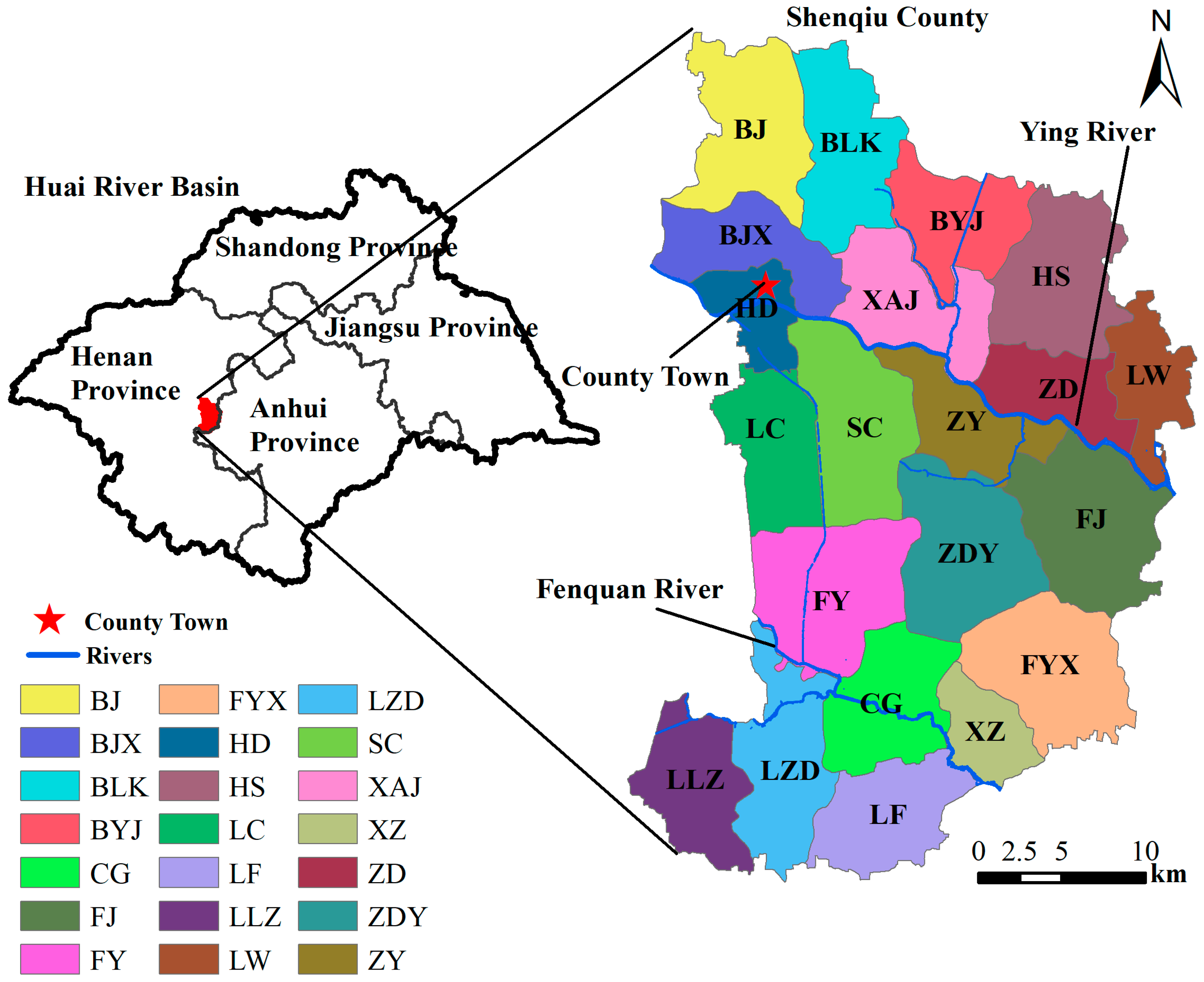
Shenqiu County (E115.07, N33.4) is situated at the center of HRB. The county covers an area of 1082 km2 and has a flat topography. Its population is 1.3 million, with a total of 21 townships (Figure 1). Geographically, Shenqiu County falls within the warm-temperate continental monsoon climate zone, characterized by distinct seasonal rainfall patterns. A significant annual precipitation (80%) occurs during the summer.
Shenqiu County is blessed with a favorable environment for agricultural production and abundant water resources. Ying River and Fenquan River run through this county, and the development of irrigation canals over the years has resulted in the proliferation of numerous ponds and canals. Nevertheless, the county’s agriculture sector has not achieved a substantial agglomeration effect. The lower level of agricultural industrialization has led to the problem of agricultural surface pollution, and combined with other reasons, has caused not only serious river pollution with low grade in water quality, but also severe eutrophication in the pond, which contains a large number of algae and algal toxins [28].
2.2. Remote Sensing Data and Processing
In this study, we employed the Advanced Land Observing Satellite (ALOS) from 2010, Gaofen-2 (GF-2) from 2016, and Gaofen-1 (GF-1) from 2022. This satellites were chosen because their images have notable attributes, including high spatial resolution and exceptional image quality, making them valuable resources for surface resource surveys [29,30,31]. While images from these three satellites are not freely available, they are cost-effective. ALOS offers a panchromatic image resolution of 2.5 m and a multispectral image resolution of 10 m. GF-1 and GF-2 represent the latest generation of Chinese high-spatial-resolution remote sensing satellites. GF-1 provides panchromatic images with a 2 m resolution and multispectral images at an 8 m resolution. GF-2 offers even higher spatial precision, with a 1 m for panchromatic images and a 4 m for multispectral images. In our image selection process, we diligently avoided cloud interference to ensure consistency of image time among ALOS, GF-2, and GF-1. Detailed information regarding these datasets is presented in Table 1. All images were acquired during non-rainy season, i.e., in February. Because there is no image of the same day on any other date that covers the entire county.
The pre-processing of ALOS, GF-2, and GF-1 images encompassed a series of crucial steps aimed at enhancing their quality and usability for subsequent analysis. These steps included radiometric calibration, atmospheric correction, ortho correction, fusion, mosaic, registration, and clipping. All steps were executed using ENVI version 5.3 software, which is easy to use. Among these steps, the Fast Line-of-Site Atmospheric Analysis of Spectral Hypercubes (FLAASH) algorithm was used for atmospheric correction, and the panchromatic images and multispectral images were then fused by NNDiffuse Pan Sharpening to obtain optical images with spatial resolution of 2.5 m, 1 m, and 2 m for ALOS, GF-2, and GF-1 images, respectively. The panchromatic images only needed radiometric correction and ortho correction.
2.3. Ponds Extraction
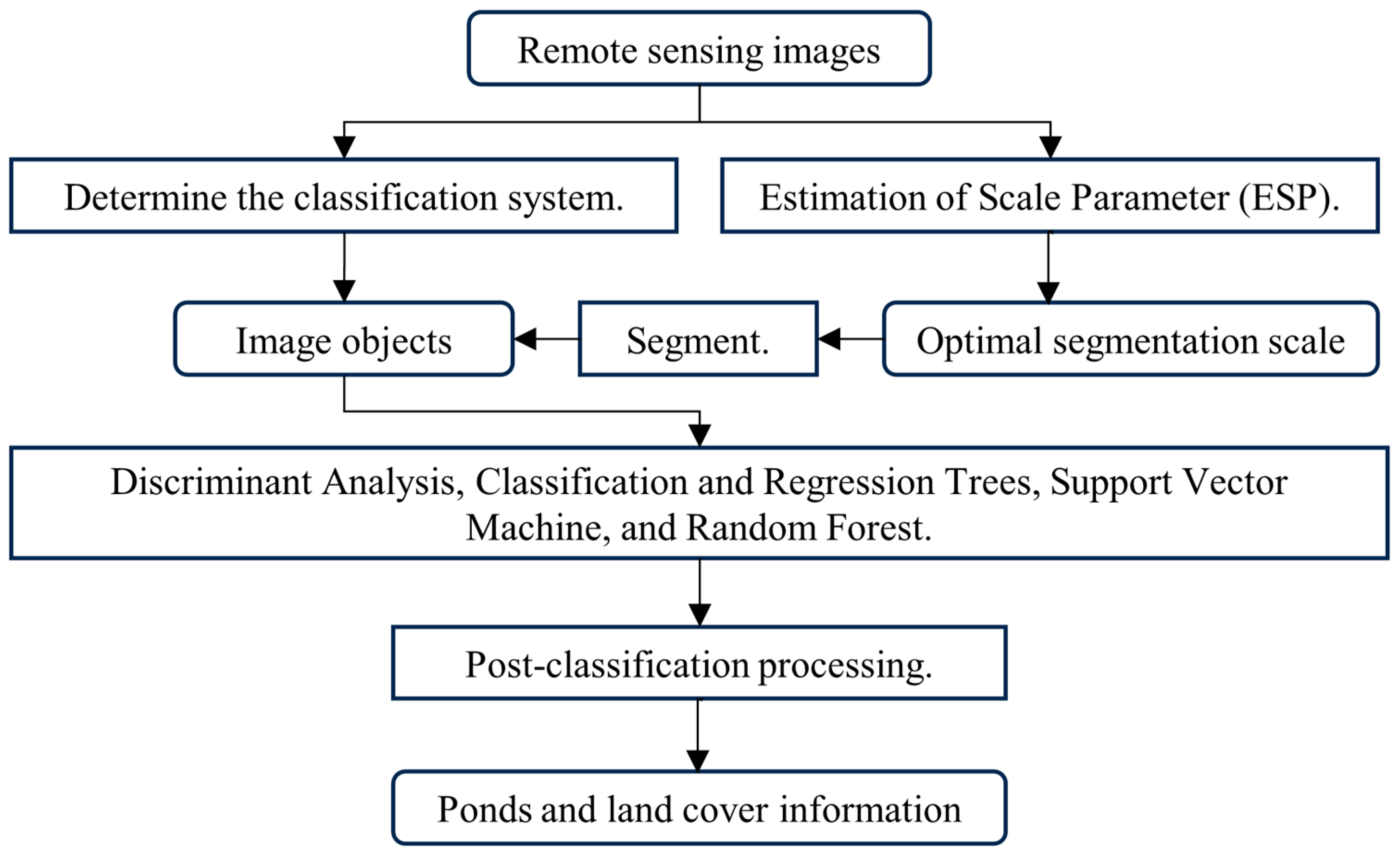
The pond information extraction process outlined in this paper comprises four primary steps (Figure 2). Initially, it involves the identification of land cover categories within the study area. Subsequently, a segmentation process is employed to obtain the image objects. Following this, a machine learning classification approach is employed. Lastly, the acquired pond information undergoes further post-processing for refinement and analysis.
2.3.1. Analysis of Surface Type
The land cover types in 2010, 2016, and 2022 were similar. Combined with the LUCC (Land-use/land-cover change) classification system and the images, the land cover types of Shenqiu County are presented in Table 2. In 2010, the classification system delineated 11 categories. However, in 2016 and 2022, the classification system was grouped into 10 categories. Compared to 2010, the classification system reduced anhydrous pond.
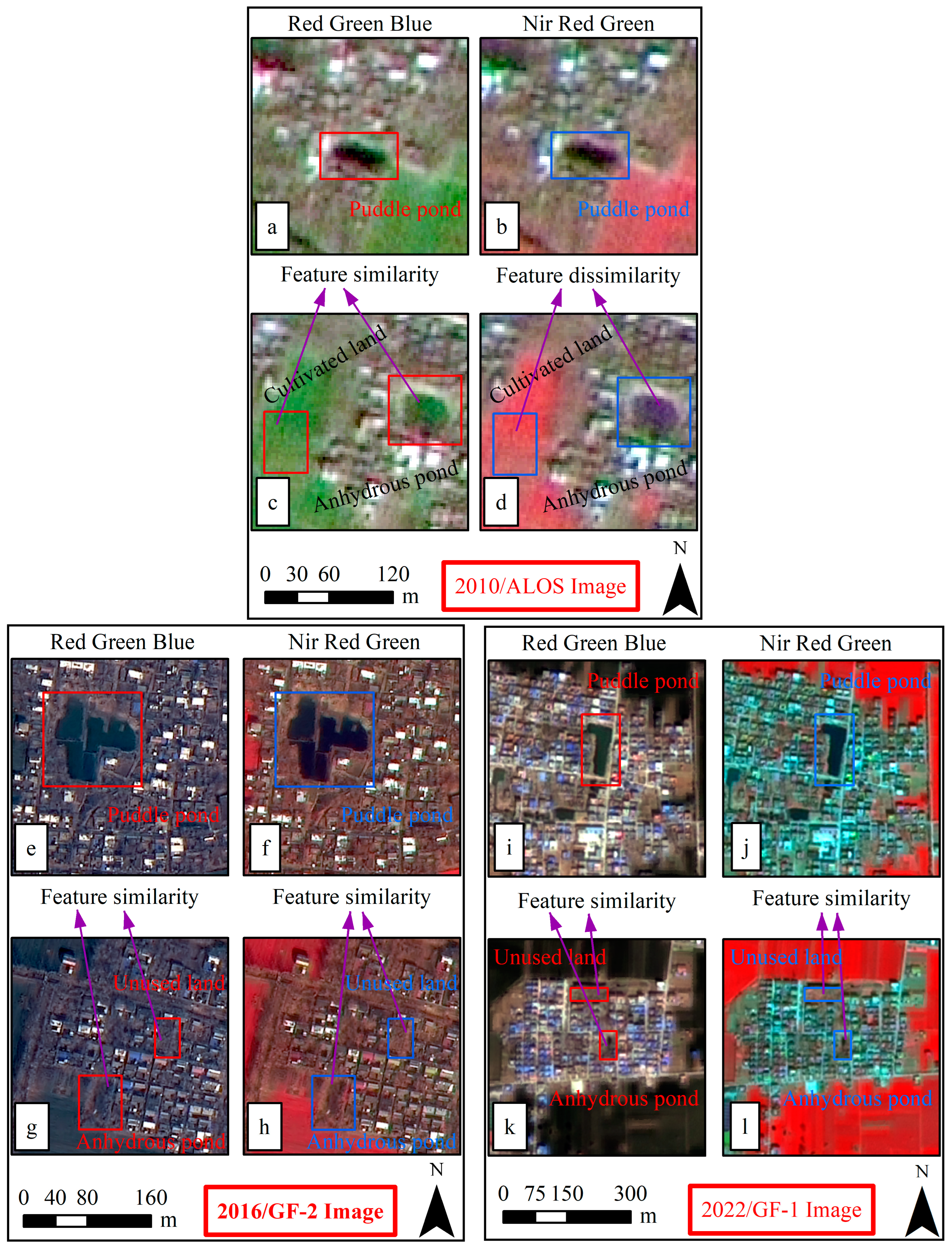
For the pond classification of 2010 images, the ponds were categorized into two distinct types: puddle pond and anhydrous pond. Anhydrous ponds are seasonal and may dry in February, during which there is no rain. The water spectral characteristics of puddle ponds were readily discernible (Figure 3a,b,e,f,i,j). In contrast, the spectral characteristics of water in anhydrous ponds are less pronounced, and these ponds were susceptible to interference from other surface types exhibiting similar spectral characteristics (Figure 3c,d,g,h,k,l).
To address this challenge, in 2010, we used the distinct coloration of anhydrous ponds in false-color representations compared to cultivated land (Figure 3c,d). Specifically, we utilized the spectral information from the Nir, Red, and Green bands for classification purposes. At the same time, we treated anhydrous ponds as an independent category during the classification process. However, in 2016 and 2022, anhydrous ponds exhibited spectral characteristics similar to those of unused land, both in true and false-color representations (Figure 3g,h,k,l). Consequently, anhydrous ponds were temporarily considered unused land. For a detailed explanation of the specific method employed for the extraction of anhydrous ponds in 2016 and 2022, please refer to Section 2.3.4.
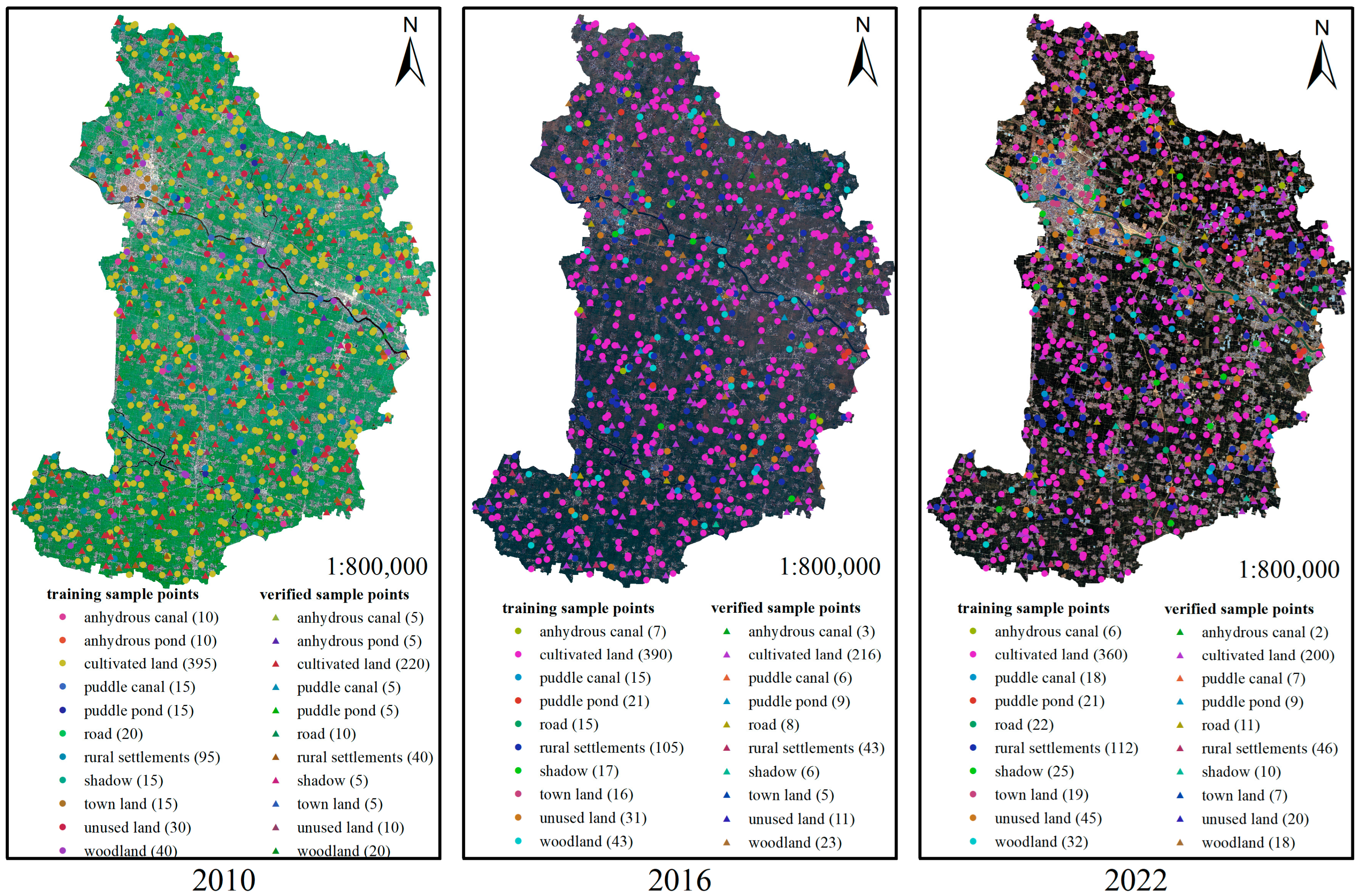
For land cover type samples, we randomly generated 990 points within the study area and adjusted sample locations based on the number of each land cover type (Figure 4). The types of these points were defined through field survey and visual interpretation. We divided these sample points into training samples and verified samples at a ratio of 2:1, which are used for training classification and evaluating the accuracy of classification results.
2.3.2. Get Image Object
The water results obtained by the extraction methods based on image pixels may exhibit a “salt and pepper” phenomenon. When the phenomenon arises, particularly when misclassified pixels are found within an object, it can substantially impact the pond’s integrity. Therefore, the object-based technique is deemed more appropriate for pond extraction [32,33,34].
Image objects consist of a contiguous group of neighboring pixels that exhibit homogeneity or the same semantic significance, attributes stemming from the process of segmentation. Segmentation is the process of partitioning the images into a spatially contiguous set of objects. Most object-oriented studies used the multiresolution segmentation algorithm in eCognition to segment images. eCognition Developer 9.0 is a proprietary software (now called Definiens Professional), which was for object-based image analysis [35]. Thus, we use this software for image segmentation. At the optimal segmentation scale, the shapes and sizes of the image objects closely resemble the actual surface characteristics corresponding to these objects. ESP (Estimation of Scale Parameter) method [36,37] in eCognition software was employed to obtain the optimal segmentation scale, ensuring both efficiency and objectivity in delineating the image objects.
2.3.3. Retrieval of Ponds Information
Discriminant Analysis (DA) is a method within the realm of multivariate statistical analysis. Its primary objective is to establish one or more discriminant functions according to various eigenvalues (independent variables) under the condition of determining sample categories (dependent variables). Then, the functions are used to identify samples of unknown categories. In this study, the fundamental unit of analysis is the segmented image object. Taking each object in the study area as a sample, the part of the image objects with identified categories were selected as training samples, which were then assigned features. Features are commonly used in object-oriented classification research [38,39] (Table 3). The discriminant functions were built based on the training samples using the DA method and employed to classify samples with undetermined categories, thereby assigning them to their appropriate categories.
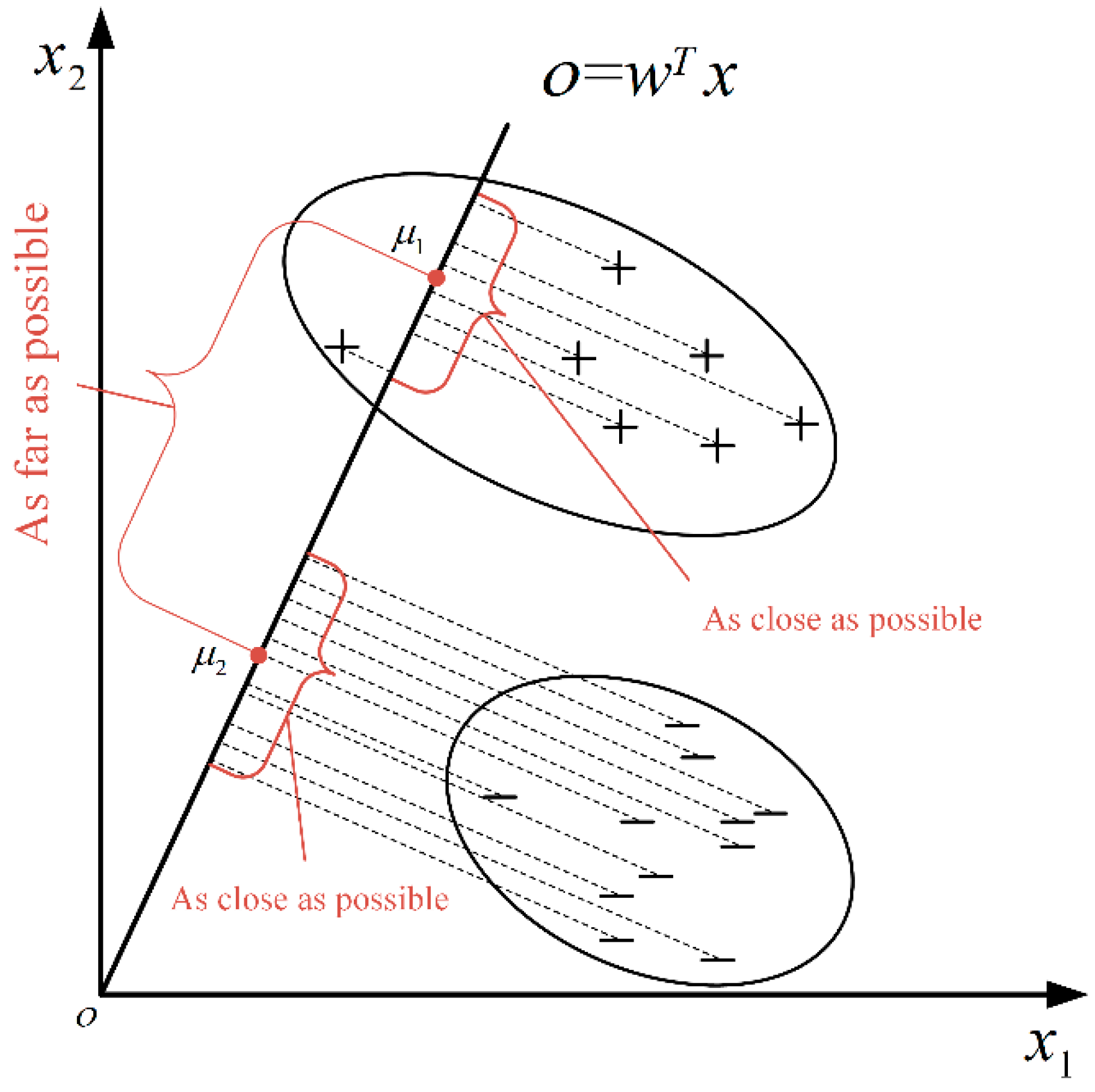
To avoid the “black box” of the classification process and discriminant functions, this study adopted the Fisher Discriminate Analysis, specifically known as Linear Discriminant Analysis (LDA). LDA utilizes linear function and Fisher value as the discriminant function and discriminant criteria, respectively. In essence, the fundamental principle underlying LDA can be succinctly encapsulated as “minimizing intra-class variance while maximizing inter-class variance upon projection”. Illustrating this concept using a training sample set comprised of two distinct types (Figure 5). This method projects the data of these two types onto a linear subspace (for more than two types, it extends to hyperplanes). Through this projection, the aim is to bring the projection points of samples belonging to the same type as close together as possible, while simultaneously maximizing the separation between projection points corresponding to different types of samples. Consequently, in the classification of novel samples, they are first projected onto this linear subspace. Subsequently, the categorization of these new samples is determined based on the position of their respective projection points.
To compare the extraction effectiveness of LDA, we employed Classification and Regression Trees (CART), Support Vector Machine (SVM), and Random Forest (RF) as control methods, which are widely used in land-cover investigations [40,41]. CART is categorized under inductive learning techniques in machine learning. The fundamental modeling process of this algorithm is to perform inductive learning on the training samples and their feature combinations. It employs the Gini index, a concept from econometrics, as the criterion to determine the optimal test feature and uses segmentation thresholds to construct a hierarchical organizational structure. This structure resembles a tree, comprised of multiple sets of leaf nodes, root nodes, and pathways. Each set represents a decision rule. When these decision rules are combined, they form a decision tree classification model. SVM is one of the most robust and frequently used supervised nonparametric statistical machine-learning methods. The fundamental principle of SVM lies in creating an optimum hyperplane also referred to as a decision boundary or optimal boundary that maximizes the distance between the nearest samples (support vectors) to the plane and effectively separates classes. The radial basis function kernel of the SVM classifier is commonly used and shows a good performance. Therefore, we used the radial basis function kernel to implement the SVM algorithm. RF is among the best and most powerful machine-learning classifiers. It is based on the principle of using decision trees as the basic classifier and creating a collective learning model by combining multiple decision trees. To enhance the comparability of results obtained through DA and CART, SVM, and RF, they employed identical sample objects for classification within the same year.
2.3.4. Post-Classification Processing
After completing the classification process, we conducted further data processing to mitigate potential omissions from ponds. This process involved several distinct steps:
- (1)
- Integration of Pond Information: We combined pond information obtained through DA, CART, SVM, and RF methods for the same year;
- (2)
- Spatial Analysis for Non-Intersecting Ponds: Subsequently, building upon the results of the preceding step, spatial analysis techniques were employed to determine the portions of ponds that did not intersect between the years 2010 and 2016, as well as between 2016 and 2022;
- (3)
- Integration with Visual Interpretation: These non-intersecting ponds were then combined with images from 2010/2016 and 2016/2022. Visual interpretation was employed to ascertain the categorization of these non-intersecting ponds, determining whether they could be classified as omission ponds, anhydrous ponds, or other surface types;
- (4)
- Validation of Omission Ponds: In the final step, a validation of omission ponds was conducted based on the extraction results and corresponding images from 2010, 2016, and 2022.
2.3.5. Accuracy Verification
Based on the image pixel-level Kappa coefficient (Kappa) and overall accuracy (OA) were then calculated using verified sample points and confusion matrixes to evaluate the accuracy of the extracted land-use information. Kappa is an index used to test whether the predicted results of the model are consistent with the actual classification results, and OA is the overall evaluation of the quality of classification results.
2.4. Analysis of Pond Characteristics
We conducted two distinct types of characteristic analyses pertaining to ponds: one focusing on hotspot aggregation regions, and the other devoted to the correlation between ponds and various land cover categories. The former method seeks to identify the primary distribution areas of ponds, while the latter method scrutinizes the spatio-temporal relations among ponds, town-village land (i.e., townland and rural settlements), and cultivated land.
In the first characterization, the fact that Shenqiu County has numerous ponds with relatively small individual areas presents a challenge to spatial analysis using administrative village boundaries. Consequently, we employed grids at varying scales and Voronoi diagrams to scrutinize the spatial distribution characteristics concerning the area and number of these ponds. Our approach commenced with the determination of the number of ponds and their respective areas within each grid and Voronoi diagram. Subsequently, we calculated the Getis-Ord Gi* regional statistics [42] for both the number and area of ponds in order to perform local spatial autocorrelation analysis to elucidate the spatial concentration patterns of ponds within the study area. Once calculated, each statistical unit will have a Z-score that plays a pivotal role in identifying statistically significant hot and cold spots. A higher absolute Z-score signified a more pronounced degree of aggregation in the number and area of ponds within this region. In this study, the hot grid unit’s significance is that the grid unit itself has very high numerical attributes for the pond parameters, and at the same time, its surrounding units also have very high numerical attributes for the pond parameters. In the second character analysis, spatiotemporal changes in the number and area of ponds within town-village land and cultivated land were analyzed.
3. Results
3.1. Accuracy and Pond Extraction Results
The accuracy of the classification results before the post-classification processing met subsequent analysis requirements in all years (Table 4, Kappa > 0.72 and OA > 76%). Most Kappa (0.75–0.84) and OA (78–84%) of DA were higher than that of CART (Kappa: 0.73–0.80, OA: 76–80%), SVM (Kappa: 0.75–0.80, OA: 77–83%), and RF (Kappa: 0.72–0.81, OA: 78–81%).
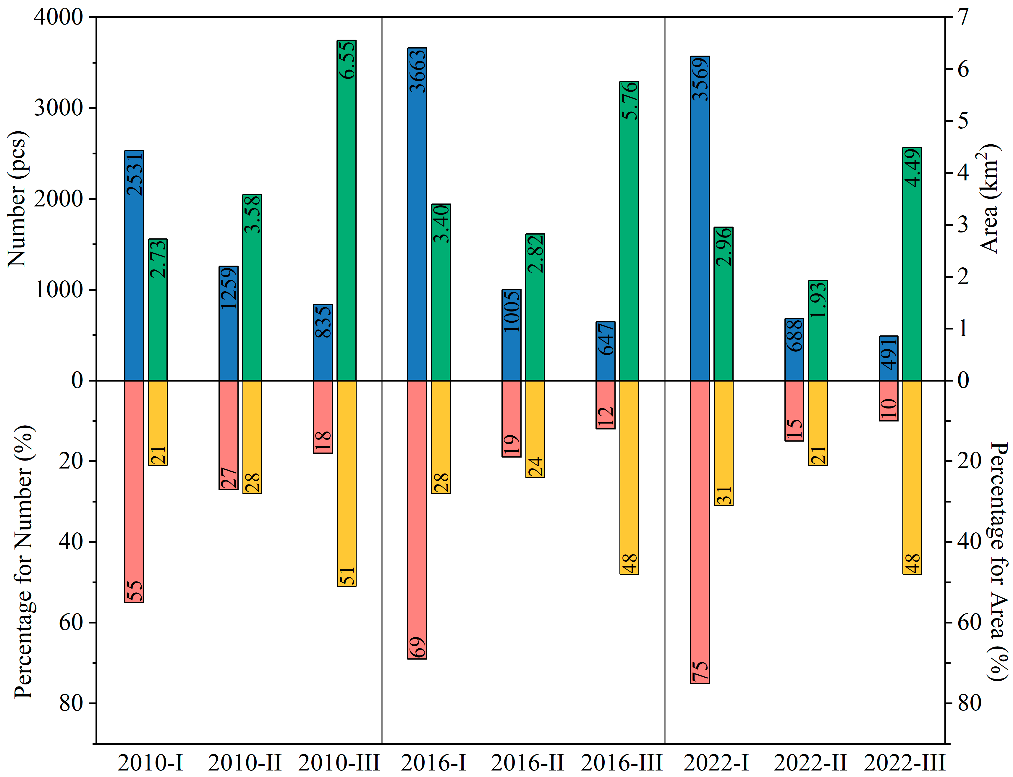
The total number of ponds in Shenqiu County accounted for 4625, 5315, and 4748 in 2010, 2016, and 2022, respectively (Figure 6). This indicated a 15% increase from 2010 to 2016, followed by an 11% decrease thereafter. In the three years, their areas were 12.86 km2 (1.19% of Shenqiu), 11.99 km2 (1.11%), and 9.37 km2 (0.87%), revealing a continuous decline of about 7% (2010–2016) and 22% (2016–2022).
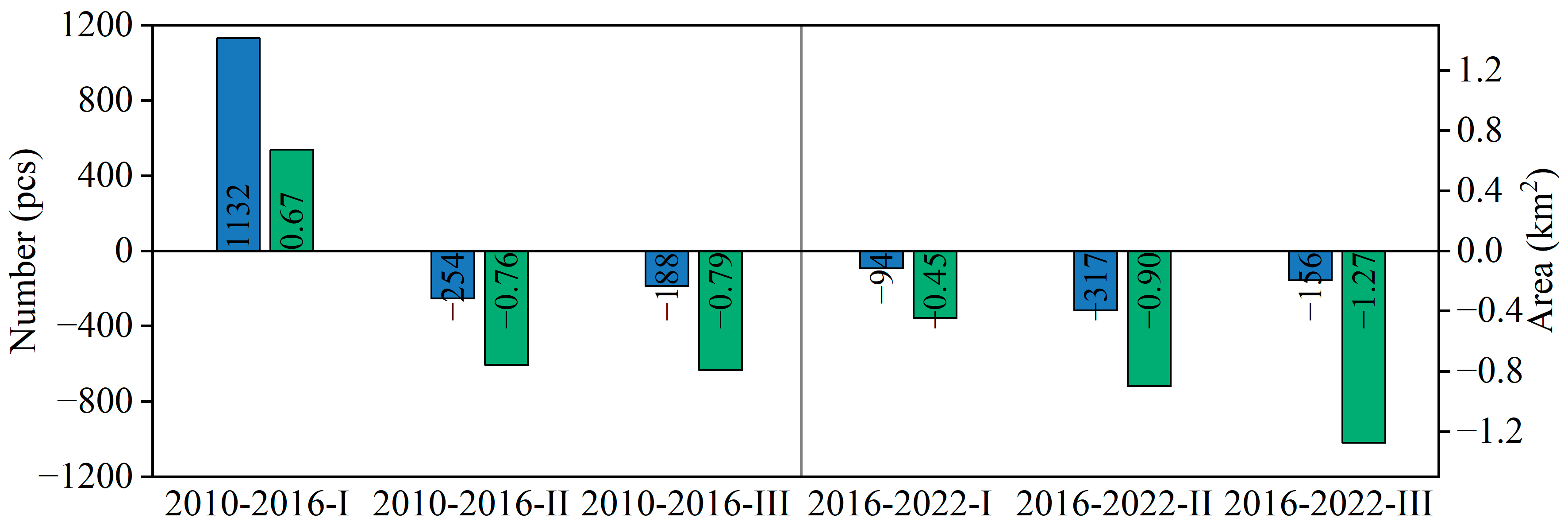
Ponds of different sizes have distinct functions and water storage capacities. We classified ponds of this study area into three levels: I (<2000 m2), II (≥2000–4000 m2), III (≥4000 m2) (Figure 6 and Figure 7). In terms of the number of ponds, level-I ponds constituted over 50% in all three periods. However, their corresponding area proportion ranged from 21% to 31%. Notably, there was an increase in 1132 ponds (total of 0.67 km2) from 2010 to 2016 and a decrease in 94 ponds (0.45 km2) from 2016 to 2022. For level-II ponds, their number proportion ranged from 15% to 27% across the three periods, with the corresponding area proportion from 21% to 28%. There was loss of 254 ponds (0.76 km2) from 2010 to 2016 and 317 ponds (0.90 km2) from 2016 to 2022. The level-III ponds have a different situation from level-I ponds. Their number proportion was consistently the smallest among the three levels, ranging from 10% to 18%. However, they accounted for the largest area proportion, constituting approximately 50% of the total pond area. The number of the level-III ponds was reduced by 188 (0.79 km2) from 2010 to 2016, and by 156 (1.27 km2) from 2016 to 2022. In summary, the overall characteristics of the ponds in this county were the presence of numerous small area ponds with a relatively modest total area and a limited number of larger ponds contributing significantly to the total area.
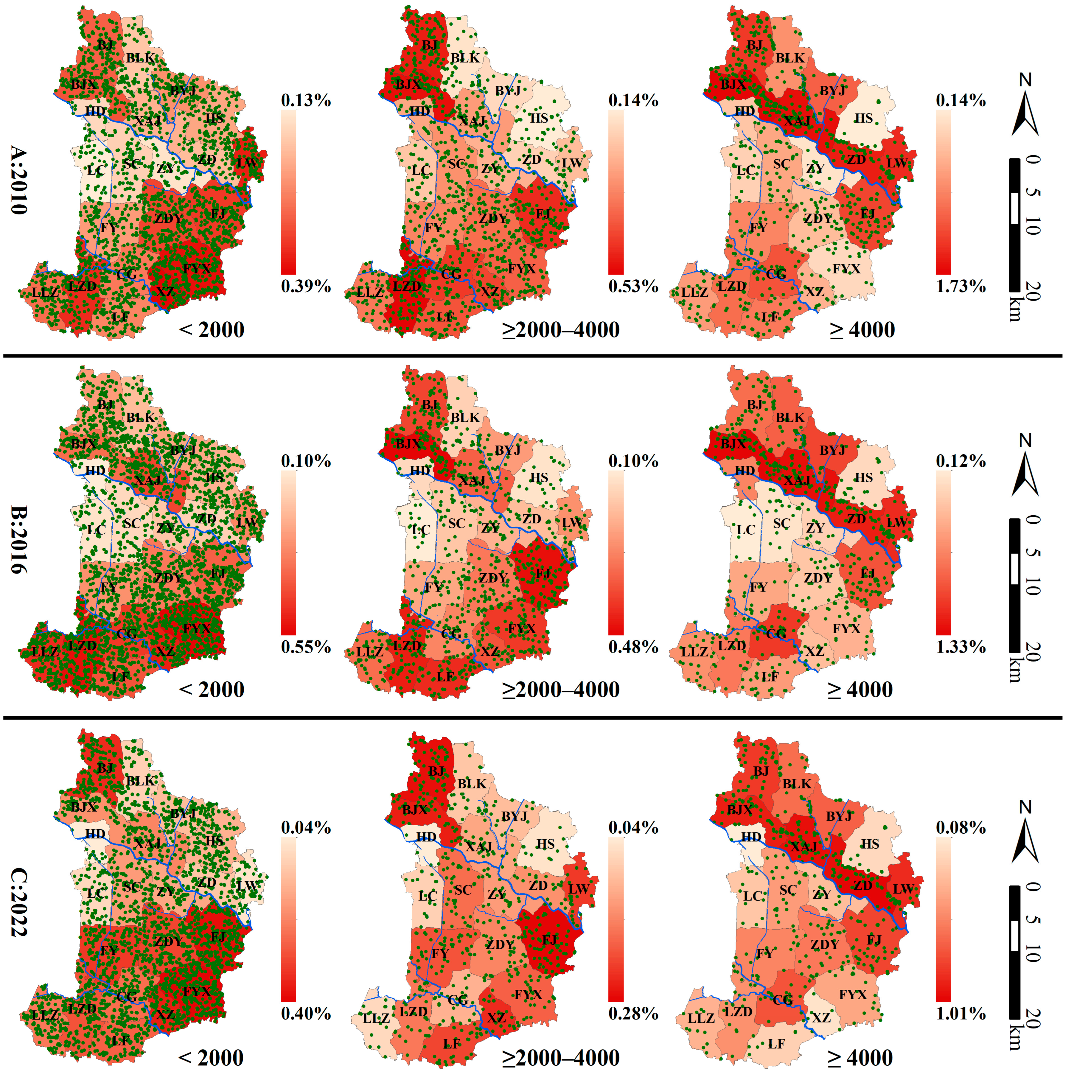
Figure 8 shows the spatial distribution of ponds, which were represented by vector points. We calculate the percentage of pond area to town area as a measure of pond density. Our results reveal a significant prevalence of ponds in Shenqiu County. Specifically, the level-I ponds were especially abundant. Most towns have a high number of ponds with relatively high area percentage values, except for the towns of LC, SC, and ZY. Interestingly, towns situated in the northwestern region of Shenqiu County and along both banks of the Fenquan River exhibited a dense distribution of the level-II ponds. Moreover, the level-III ponds were primarily concentrated in towns located in the northern vicinity of the Yinghe River, forming a narrow, belt-shaped area. These results indicated that the main characteristic of pond distribution in Shenqiu was the dense presence of the level-I ponds.
3.2. Distribution of Hot Spots in Ponds
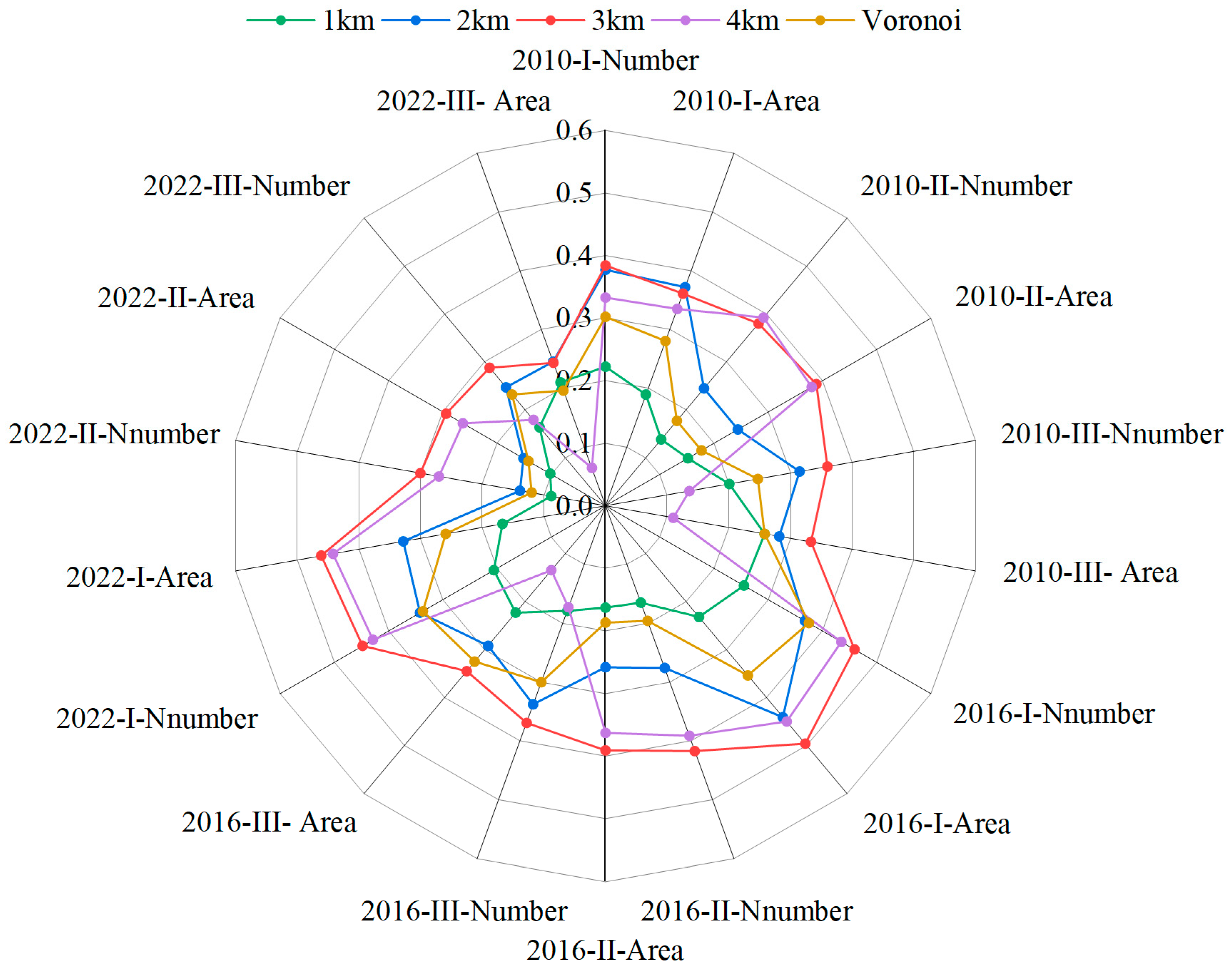
The spatial autocorrelation, measured by Moran’s I index at the 1–4 km grid scales and the Voronoi diagram, for both the number and area of ponds ranged from 0.1 to 0.5 and exhibited statistical significance (p-value < 0.1, Z-score > 2.58) (Figure 9). The Voronoi diagram was generated using GIS software, which employed village points as input in its computation. The results indicated that the pond distribution had a discernible spatial autocorrelation, showing a clustering distribution. Except for 2010-I-Area, 2010-II-Number, and 2022-III-Area, Moran’s I values for both pond number and area were consistently higher at the 3 km grid scale. Consequently, the 3 km grid was identified as the most suitable unit of autocorrelation analysis.
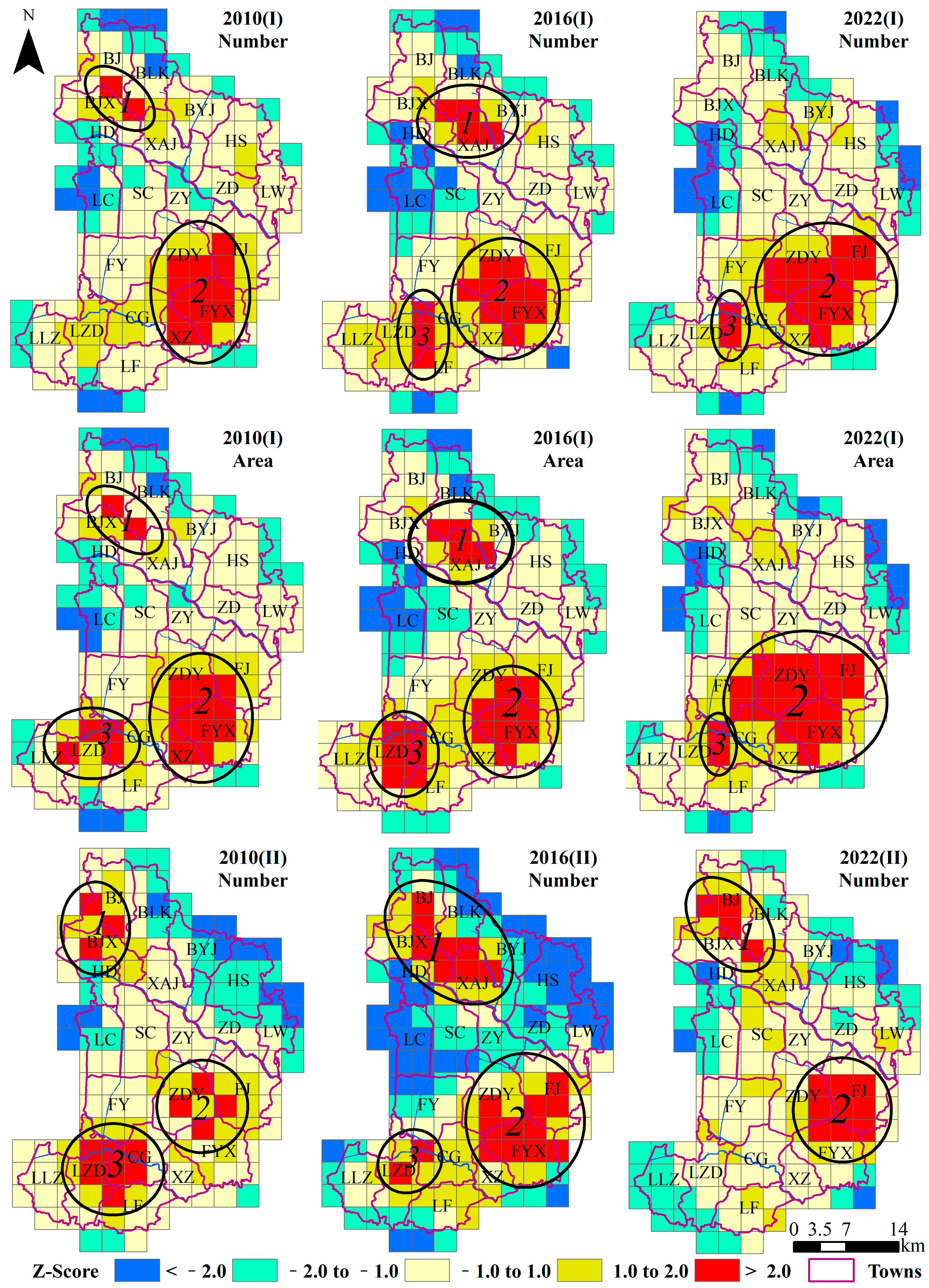
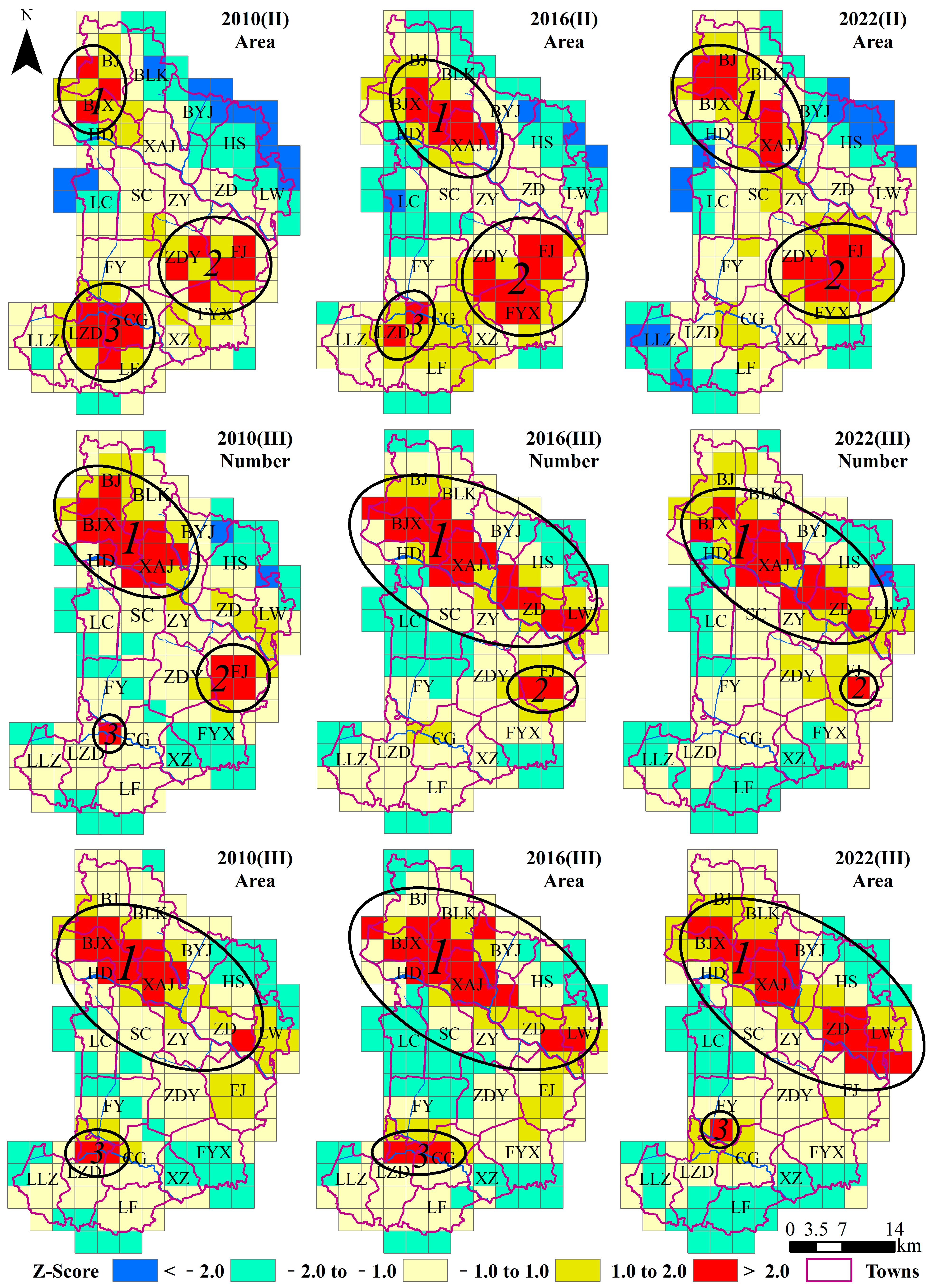
The hot spot analysis results at the 3 km grid scale (Figure 10) displayed that all three levels of ponds presented pronounced spatial aggregation characteristics, and the high-value hot spot grids (Z-score > 2) were concentrated in three distinct clustered areas. The first cluster area was predominantly located to the north of the Ying River, that is the north or northwest of the county. The second cluster area was primarily located in the southeast region of the county. The third cluster area was mostly situated in the south, and the Fenquan River flows through this area. The level-III ponds were most widely distributed in the first area, whereas the second and third areas were primarily dominated by level-I and level-II ponds. From 2010 to 2022, except for the first cluster area of level-I ponds, the third cluster area of level-II ponds, and the third cluster area of the number of level-III ponds had vanished, the cluster areas of other ponds had been always in existence.
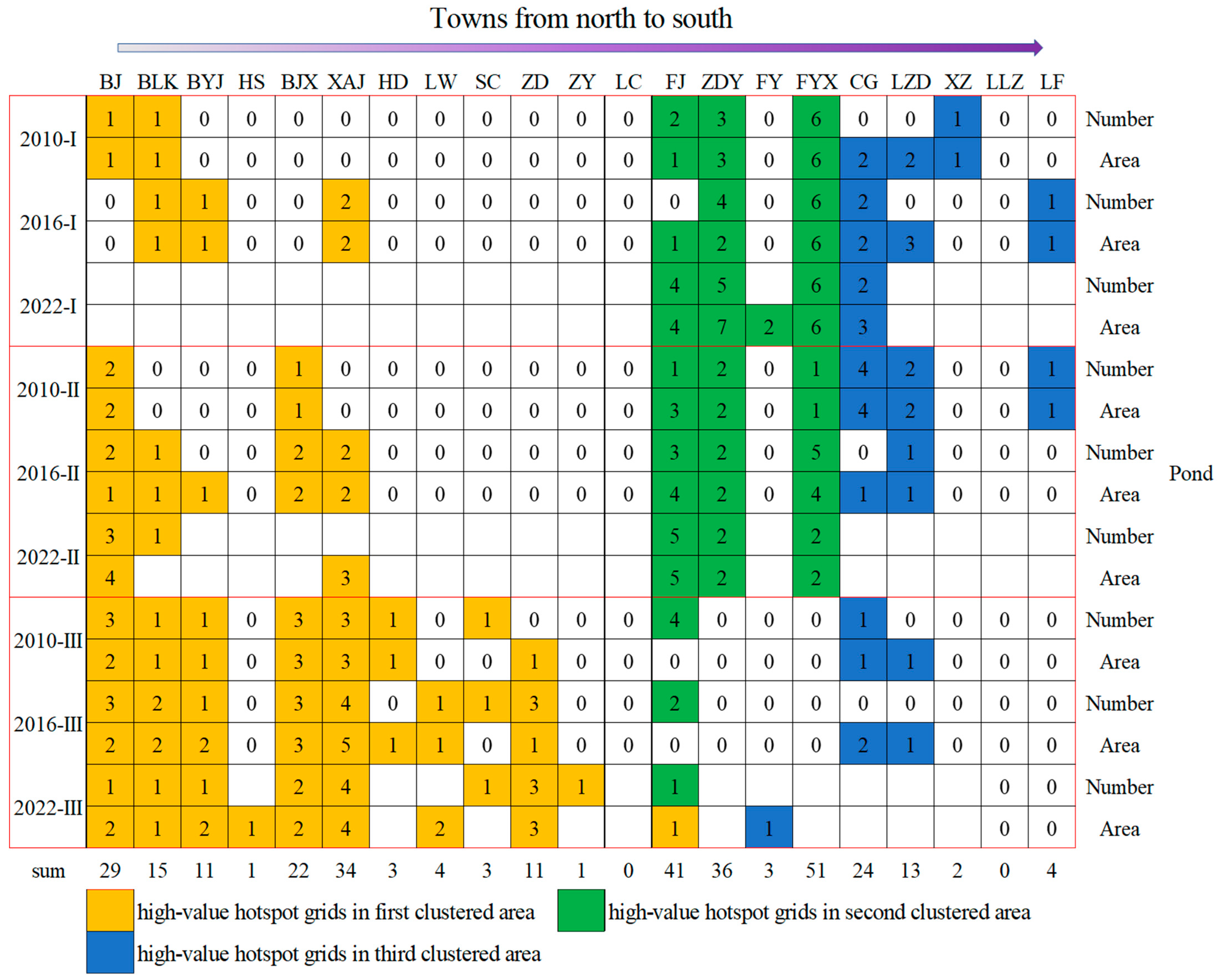
To identify towns with high-value hotspot grids, we counted the number of such grids within each town based on the center coordinates of each grid (Figure 11). FYX, FJ, ZDY, XAJ, BJ, CG, and BJX have a large number of high-value hotspot grids, with a total of 51, 41, 36, 34, 29, 24, and 22 grids, respectively. Conversely, other towns recorded fewer than 20 high-value hotspot grids each. It is noteworthy that towns situated in the northern region exhibited a significant concentration of high-value hotspot grids on level-III ponds, while those in the southern region are concentrated on level-I and level-II ponds.
The number of high-value hotspot grids per town changed from 2010 to 2022. Specifically, for level-I ponds, the high-value hotspot grids ceased to exist in BJ, BLK, LZD, and XZ. Conversely, they were first present and subsequently vanished in BYJ, XAJ, and LF. It’s worth noting that they remained consistently prevalent in FJ, ZDY, FYX, and CG. Regarding level-II ponds, the high-value hotspot grids were not found in BJX, CG, LZD, and LF, while they were first observed and subsequently disappeared in BLK and XAJ. However, they consistently persisted in BJ, FJ, ZDY, and FYX. Regarding level-III ponds, the high-value hotspot grids ceased to exist for HD, CG, and LZD, but were introduced in LW, while they remained an enduring feature in BJ, BLK, BYJ, BJX, XAJ, SC, ZD, and FJ.
3.3. Spatial-Temporal Relationships between Ponds, Town-Village Land, and Cultivated Land
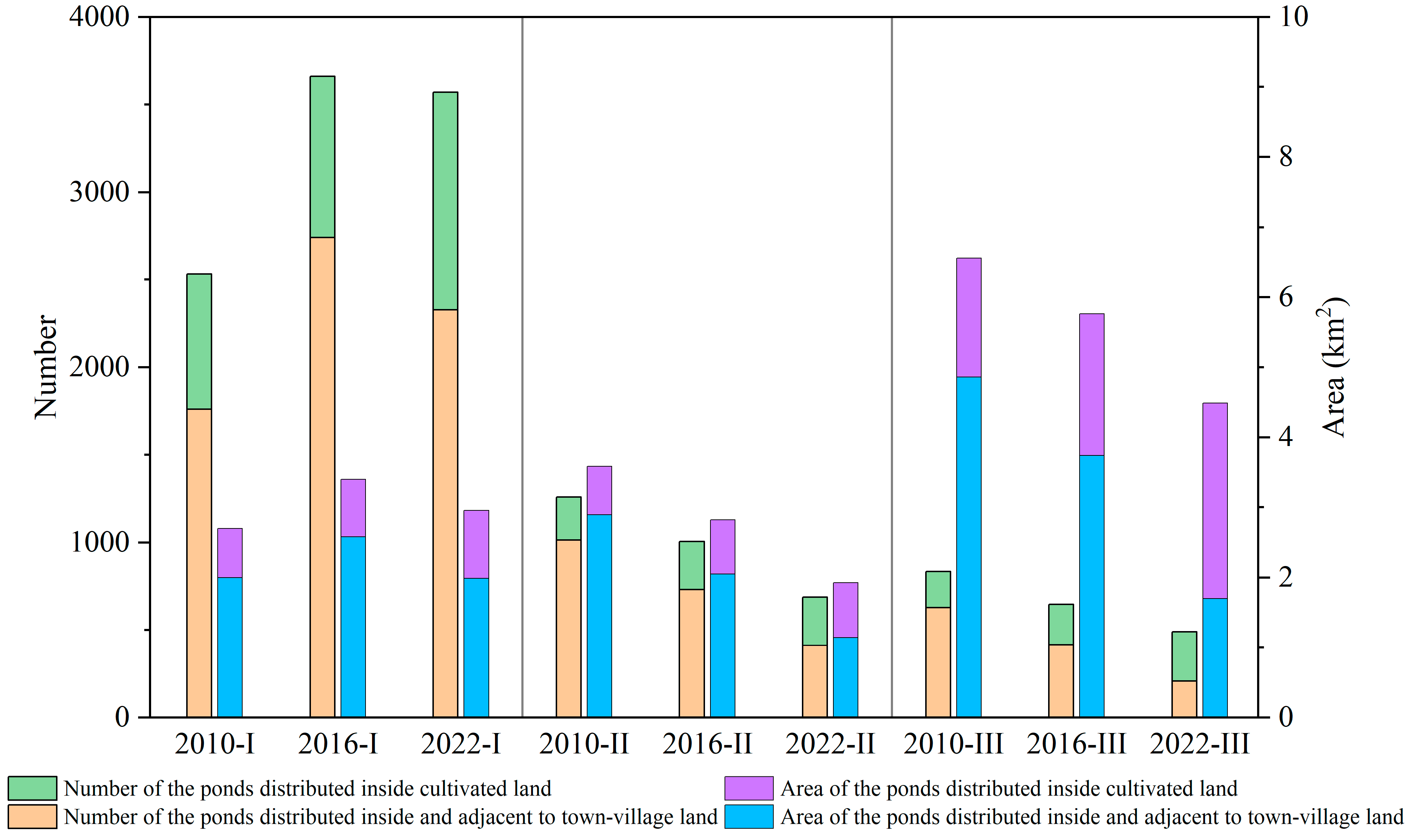
We have identified another salient characteristic in the spatial distribution of ponds, namely their strong association with town-village land (i.e., townland and rural settlements) and cultivated land. Town-village land and cultivated land hold significance in the lives of residents and agricultural production. Thereby, rendering the quantity and extent of ponds of paramount importance. Figure 12 shows the pond number and area situated within and adjacent to town-village land and within cultivated land. It can be found that the pond number and area within and adjacent to town-village land far exceeded those situated within cultivated land. From 2010 to 2016, there was an increase in both the number and area of level-I ponds within cultivated land, as well as those within and adjacent to town-village land. However, the latter experienced a notably more substantial increment compared to the former. In contrast, between 2016 and 2022, we observed a decrease in the number and area of level-I ponds within and adjacent to town-village land, while those within cultivated land witnessed an increase. From 2010 to 2022, there was a small increase in the number and area of level II and III ponds situated within cultivated land. In the same period, however, there was a considerable reduction in both the number and area of ponds located within and adjacent to town-village land.
4. Discussion
The quantity, area, distribution, and change of ponds are essential to monitor and evaluate regional water environmental health. In this paper, we employ DA-based image objects to identify ponds and analyze their spatial-temporal changes using high-resolution remote sensing data from the years 2010, 2016, and 2022 in Shenqiu County, located in HRB, China. This study has several remarkable findings. Our study contributes significantly by offering valuable methodological support for the ecological monitoring and management of water environments in regions characterized by a dense concentration of ponds. Furthermore, the outcomes related to ponds furnish crucial data that can inform both environmental and social development initiatives within the area.
4.1. Method Applicability
Results in this paper indicated that DA based on an object-oriented extraction is a valuable machine learning method for classifying and extracting information related to land surface, especially ponds. This study first used the optimal segmentation scale to segment images into objects, thereby ensuring the integrity of pond objects to the greatest extent. Subsequently, land surface information was extracted from these image objects using DA. The accuracy evaluation results showed the higher performance of DA over CART, SVM, and RF.
Two factors were identified as challenges in the process of pond extraction and the application of the extraction model. The first was the spectral similarity of the pond with some land cover types, particularly shadow and unused land. This often resulted in unavoidable misclassification between these land cover types. Although these misclassified objects were corrected in subsequent post-processing steps in this study, there is still a need to investigate fast and effective methods to avoid this misclassification in the future. In addition, DA selects characteristics (parameters) for each land cover type to establish the discriminant function based on the conditions of the study area. However, there are differences in the number and spectral characteristics of land cover types across geographic regions. Thus, the discriminant functions obtained for the same land cover category may vary in different geographical areas, which makes it difficult for the discriminant functions model to be transferred and applied among the heterogenous landscape.
Two areas were improved as much as possible during pond monitoring. First, while the post-processing strategy employed in this study undeniably guarantees the extraction results of the anhydrous pond and enhances overall pond detection accuracy, it is essential to acknowledge its relatively lower efficiency. It is advisable to use image data from the rainy season extensively in research endeavors to bolster both the efficiency and precision of pond extraction, particularly for anhydrous ponds. The reason why we did not use images from multiple dates during the rainy season is that this study used a supervised classification method, and the same surface type in images from the same date has similar spectral characteristics. Using these images ensures that the established model based on samples and supervised classification methods can accurately extract surface information as accurately as possible for the entire study area. Second, the difference in image resolution between the three periods leads to deviations in the size and shape of the extracted ponds, potentially influencing the number and area results and analysis of ponds [43]. It is recommended for future studies to prioritize the use of high-resolution images acquired from the same platform whenever feasible.
4.2. Pond Environment in the Study Area
Ponds constitute an integral component of the rural ecology and the human settlement landscape in Shenqiu County, with a substantial presence and wide distribution across the county region. From 2010 to 2016, the overall number of ponds increased, however, the total area decreased. Of these, there was a notable increase in both the number and area of level-I ponds. Conversely, the number and area of level-II and level-III ponds exhibited a decline during this period. This phenomenon is not only due to the relatively coarse spatial resolution of the ALOS image in 2010, which does not adequately describe ponds of small areas but may also be related to some degree of treatment of large area ponds. Subsequently, from 2016 to 2022, there was a discernible reduction in both the number and area of ponds. This decline is related to environmental management during this period. As the contaminated water seriously affects the safety of residents, the relevant departments have carried out continuous remediation of the ponds, such as the filling of some contaminated ponds.
This study also found an apparent agglomeration effect of ponds on the 3 km grid scale, primarily concentrated within three specific regions. The first cluster area is located in the county seat and the north bank of the river, and the third cluster area is situated in the old county seat. The dense distribution of ponds in these areas may be related to economic and agricultural development. The second cluster area is positioned amidst two rivers, which may be related to the agricultural development in this area. We also counted the number of hotspot grids corresponding to the clustered areas within each town. From 2010 to 2022, the number of hotspot grids per town changed, and hotspot grids began to present in some towns, hotspot grids have vanished in some towns, and hotspot grids have consistently existed in some towns. It can be found that the scope of the clustering areas has changed. The towns with a high number of hotspot grids and the areas that have always been hotspot grids need to be focused on.
Furthermore, we also discovered that the ponds in this county region are interspersed with town-village and cultivated land, forming closely intertwined connections with the production and daily lives of residents (Figure 12). Research has illuminated that the HRB grapples with severe water environmental pollution and elevated mortality rates due to malignant tumors in the digestive tract, with Shenqiu County, situated in the central HRB, bearing a particularly heavy burden in this regard [9]. The situation is the infiltration of various pollutants into surface water and groundwater in diverse forms, leading to a significant degradation of water quality. Pond water bodies, characterized by their limited renewal capacity, are prone to becoming breeding grounds for pathogenic microorganisms and parasites [9]. Level-I ponds, in particular, had a relatively small space with poorer capabilities in water storage and self-purification. From 2010 to 2022, the presence of these ponds has had a detrimental impact on the ecological health of Shenqiu County. Nonetheless, it is encouraging to note that, between 2016 and 2022, the number of ponds distributed within and adjacent to town-village land has declined. Among them, the significant reduction of level-II and III ponds within and adjacent to the town-village land contributes positively to the safety and well-being of residents. In light of these findings, we recommend reinforcing the monitoring and governance of ponds in these clustered regions to facilitate the enhancement of the rural ecological environment and the improvement of human settlement quality. It is essential to emphasize that this work is also a focus of the current beautiful rural construction work in China.
5. Conclusions
In this paper, we employed linear discriminant analysis, classification and regression tree, support vector machine, and random forest to extract the ponds based on object-oriented with the high-resolution images (ALOS in 2010, GF-2 in 2016, and GF-1 in 2022) in Shenqiu County, and further analyzed the spatial-temporal variations of the ponds. Our results showed that the linear discriminant analysis based on image objects can effectively extract land surface information of Shenqiu County from high-resolution remote sensing data with the best accuracy among the four methods. There are 4625, 5315, and 4748 ponds in 2010, 2016, and 2022, respectively, that were widely distributed in Shenqiu County. In the initial period (2010 to 2016), there was an increase in the number of ponds, followed by a decrease in the second period (2016–2022). Approximately 1% of the county’s total area is covered by ponds. We found that there were three highly clustered areas of ponds. The first, second, and third cluster areas were predominantly located in the north or northwest, southeast, and south separately of the county. From 2010 to 2022, these cluster areas had been always in existence and were mainly in FYX, FJ, ZDY, XAJ, BJ, CG, and BJX towns. These towns need to pay more attention to their pond environment. In the future, we can use remote sensing to monitor water quality in ponds based on the results of this paper. Ponds constitute a pivotal component of aquatic ecosystems and play an important role in many aspects such as environmental beautification and economic development. We suggest that local government departments such as environmental and health institutions should strengthen the monitoring and management of ponds and focus on the effective utilization and improvement of water environments in ponds.
Author Contributions
Conceptualization, methodology, formal analysis, writing—original draft and funding acquisition, Z.J.; writing—review and editing, investigation, validation, resources and supervision, H.R.; resources, C.Z.; writing—review and editing, E.S.A. All authors have read and agreed to the published version of the manuscript.
Funding
This research was funded by the Research Foundation of Liaocheng University (No. 318052254).
Data Availability Statement
The data presented in this study are available on request from the corresponding author.
Conflicts of Interest
Author C.Z. is employed by Beijing Goldenwater Information Technology Co., Ltd. The remaining authors declare that the research was conducted in the absence of any commercial or financial relationships that could be construed as a potential conflict of interest.
References
- Cereghino, R.; Biggs, J.; Oertli, B.; Declerck, S. The ecology of European ponds: Defining the characteristics of a neglected freshwater habitat. Hydrobiologia 2008, 597, 1–6. [Google Scholar] [CrossRef]
- Peng, K.; Jiang, W.; Hou, P.; Wu, Z.; Ling, Z.; Wang, X.; Niu, Z.; Mao, D. Continental-scale wetland mapping: A novel algorithm for detailed wetland types classification based on time series Sentinel-1/2 images. Ecol. Indic. 2023, 148, 110113. [Google Scholar] [CrossRef]
- Chen, W.; He, B.; Nover, D.; Lu, H.; Liu, J.; Sun, W.; Chen, W. Farm ponds in southern China: Challenges and solutions for conserving a neglected wetland ecosystem. Sci. Total Environ. 2019, 659, 1322–1334. [Google Scholar] [CrossRef]
- Phillips, G.; Bramwell, A.; Pitt, J.; Stansfield, J.; Perrow, M. Practical application of 25 years’ research into the management of shallow lakes. Hydrobiologia 1999, 395–396, 61–76. [Google Scholar] [CrossRef]
- Liu, X.; Xu, H.; Wang, X.; Wu, Z.; Bao, X. An ecological engineering pond aquaculture recirculating system for effluent purification and water quality control. CLEAN–Soil Air Water 2014, 42, 221–228. [Google Scholar] [CrossRef]
- De Meester, L.; Declerck, S.; Stoks, R.; Louette, G.; Van de Meutter, F.; De Bie, T.; Michels, E.; Brendonck, L. Ponds and pools as model systems in conservation biology, ecology and evolutionary biology. Aquat. Conserv.-Mar. Freshw. Ecosyst. 2005, 15, 715–725. [Google Scholar] [CrossRef]
- Downing, J.A. Emerging global role of small lakes and ponds: Little things mean a lot. Limnetica 2010, 29, 9–24. [Google Scholar] [CrossRef]
- Oertli, B.; Biggs, J.; Cereghino, R.; Grillas, P.; Joly, P.; Lachavanne, J.B. Conservation and monitoring of pond biodiversity: Introduction. Aquat. Conserv.-Mar. Freshw. Ecosyst. 2005, 15, 535–540. [Google Scholar] [CrossRef]
- Ren, H.; Xu, D.; Shi, X.; Xu, J.; Zhuang, D.; Yang, G. Characterisation of gastric cancer and its relation to environmental factors: A case study in Shenqiu County, China. Int. J. Environ. Health Res. 2016, 26, 1–10. [Google Scholar] [CrossRef]
- Tian, D.; Zheng, W.; Wei, X.; Sun, X.; Liu, L.; Chen, X.; Zhang, H.; Zhou, Y.; Chen, H.; Zhang, H. Dissolved microcystins in surface and ground waters in regions with high cancer incidence in the Huai River Basin of China. Chemosphere 2013, 91, 1064–1071. [Google Scholar] [CrossRef]
- Xie, H.; Xin, L.; Xiong, X.; Tong, X.; Zhou, B. New hyperspectral difference water index for the extraction of urban water bodies by the use of airborne hyperspectral images. J. Appl. Remote Sens. 2014, 8, 085098. [Google Scholar] [CrossRef]
- Zhou, Y.; Dong, J.; Xiao, X.; Xiao, T.; Yang, Z.; Zhao, G.; Zou, Z.; Qin, Y. Open surface water mapping algorithms: A comparison of water-related spectral indices and sensors. Water 2017, 9, 256. [Google Scholar] [CrossRef]
- Verpoorter, C.; Kutser, T.; Tranvik, L. Automated Mapping of Water Bodies Using Landsat Multispectral Data. Limnol. Oceanogr. Methods 2012, 10, 1037–1050. [Google Scholar] [CrossRef]
- Lacaux, J.P.; Tourre, Y.M.; Vignolles, C.; Ndione, J.A.; Lafaye, M. Classification of ponds from high-spatial resolution remote sensing: Application to Rift Valley Fever epidemics in Senegal. Remote Sens. Environ. 2007, 106, 66–74. [Google Scholar] [CrossRef]
- Gusmawati, N.F.; Cheng, Z.; Soulard, B.; Lemonnier, H.; Selmaouifolcher, N. Aquaculture Pond Precise Mapping in Perancak Estuary, Bali, Indonesia. J. Coast. Res. 2016, 1, 637–641. [Google Scholar] [CrossRef]
- Gusmawati, N.; Soulard, B.; Selmaoui-Folcher, N.; Proisy, C.; Mustafa, A.; Le Gendre, R.; Laugier, T.; Lemonnier, H. Surveying shrimp aquaculture pond activity using multitemporal VHSR satellite images-case study from the Perancak estuary, Bali, Indonesia. Mar. Pollut. Bull. 2018, 131, 49–60. [Google Scholar] [CrossRef]
- Jawak, S.D.; Luis, A.J. A Rapid Extraction of Water Body Features from Antarctic Coastal Oasis Using Very High-Resolution Satellite Remote Sensing Data. Aquat. Procedia 2015, 4, 125–132. [Google Scholar] [CrossRef]
- Soti, V.; Puech, C.; Seen, D.L.; Bertran, A.; Vignolles, C.; Mondet, B.; Dessay, N.; Tran, A. The potential for remote sensing and hydrologic modelling to assess the spatio-temporal dynamics of ponds in the Ferlo Region (Senegal). Hydrol. Earth Syst. Sci. 2010, 14, 1449–1464. [Google Scholar] [CrossRef]
- Loberternos, R.A.; Porpetcho, W.P.; Graciosa, J.C.A.; Violanda, R.R.; Diola, A.G.; Dy, D.T.; Otadoy, R.E.S. An Object-Based Workflow Developed to Extract Aquaculture Ponds from Airborne LIDAR Data: A Test Case in Central Visayas, Philippines. ISPRS-Int. Arch. Photogramm. Remote Sens. Spat. Inf. Sci. 2016, XLI-B8, 1147–1152. [Google Scholar] [CrossRef]
- Prasad, K.A.; Ottinger, M.; Wei, C.; Leinenkugel, P. Assessment of Coastal Aquaculture for India from Sentinel-1 SAR Time Series. Remote Sens. 2019, 11, 357. [Google Scholar] [CrossRef]
- Xie, C.; Huang, X.; Zeng, W.; Fang, X. A novel water index for urban high-resolution eight-band WorldView-2 imagery. Int. J. Digit. Earth 2016, 9, 925–941. [Google Scholar] [CrossRef]
- Bandos, T.V.; Bruzzone, L.; Camps-Valls, G. Classification of Hyperspectral Images with Regularized Linear Discriminant Analysis. IEEE Trans. Geosci. Remote Sens. 2009, 47, 862–873. [Google Scholar] [CrossRef]
- Sheykhmousa, M.; Mahdianpari, M.; Ghanbari, H.; Mohammadimanesh, F.; Ghamisi, P.; Homayouni, S. Support vector machine versus random forest for remote sensing image classification: A meta-analysis and systematic review. IEEE J. Sel. Top. Appl. Earth Obs. Remote Sens. 2020, 13, 6308–6325. [Google Scholar] [CrossRef]
- Pelletier, C.; Valero, S.; Inglada, J.; Champion, N.; Dedieu, G. Assessing the robustness of Random Forests to map land cover with high resolution satellite image time series over large areas. Remote Sens. Environ. 2016, 187, 156–168. [Google Scholar] [CrossRef]
- Imani, M.; Ghassemian, H. Feature space discriminant analysis for hyperspectral data feature reduction. ISPRS J. Photogramm. Remote Sens. 2015, 102, 1–13. [Google Scholar] [CrossRef]
- Chen, R.; Dewi, C.; Huang, S.; Caraka, R.E. Selecting critical features for data classification based on machine learning methods. J. Big Data 2020, 7, 52. [Google Scholar] [CrossRef]
- Chen, M.; Wang, Q.; Li, X. Discriminant Analysis with Graph Learning for Hyperspectral Image Classification. Remote Sens. 2018, 10, 836. [Google Scholar] [CrossRef]
- Ji, W.; Zhuang, D.; Ren, H.; Jiang, D.; Huang, Y.; Xu, X.; Chen, W.; Jiang, X. Spatiotemporal variation of surface water quality for decades: A case study of Huai River System, China. Water Sci. Technol. J. Int. Assoc. Water Pollut. Res. 2013, 68, 1233–1241. [Google Scholar] [CrossRef]
- Wang, H.; Wang, C.; Wu, H. Using GF-2 Imagery and the Conditional Random Field Model for Urban Forest Cover Mapping. Remote Sens. Lett. 2016, 7, 378–387. [Google Scholar] [CrossRef]
- Liu, M.; Fu, B.; Xie, S.; He, H.; Lan, F.; Li, Y.; Lou, P.; Fan, D. Comparison of multi-source satellite images for classifying marsh vegetation using DeepLabV3 Plus deep learning algorithm. Ecol. Indic. 2021, 125, 107562. [Google Scholar] [CrossRef]
- Cheng, B.; Liang, C.; Liu, X.; Liu, Y.; Ma, X.; Wang, G. Research on a novel extraction method using Deep Learning based on GF-2 images for aquaculture areas. Int. J. Remote Sens. 2020, 41, 3575–3591. [Google Scholar] [CrossRef]
- Virdis, S.G.P. An object-based image analysis approach for aquaculture ponds precise mapping and monitoring: A case study of Tam Giang-Cau Hai Lagoon, Vietnam. Environ. Monit. Assess. 2014, 186, 117–133. [Google Scholar] [CrossRef]
- Zhang, T.; Yang, X.; Hu, S.; Su, F. Extraction of Coastline in Aquaculture Coast from Multispectral Remote Sensing Images: Object-Based Region Growing Integrating Edge Detection. Remote Sens. 2013, 5, 4470–4487. [Google Scholar] [CrossRef]
- Ji, Z.; Zhu, Y.; Pan, Y.; Zhu, X.; Zheng, X. Large-Scale Extraction and Mapping of Small Surface Water Bodies Based on Very High-Spatial-Resolution Satellite Images: A Case Study in Beijing, China. Water 2022, 14, 2889. [Google Scholar] [CrossRef]
- Lourenço, P.; Teodoro, A.C.; Gonçalves, J.A.; Honrado, J.P.; Cunha, M.; Sillero, N. Assessing the performance of different OBIA software approaches for mapping invasive alien plants along roads with remote sensing data. Int. J. Appl. Earth Obs. Geoinf. 2021, 95, 102263. [Google Scholar] [CrossRef]
- Drăguţ, L.; Csillik, O.; Eisank, C.; Tiede, D. Automated parameterisation for multi-scale image segmentation on multiple layers. ISPRS J. Photogramm. Remote Sens. Off. Publ. Int. Soc. Photogramm. Remote Sens. 2014, 88, 119. [Google Scholar] [CrossRef]
- Drǎguţ, L.; Tiede, D.; Levick, S.R. ESP: A tool to estimate scale parameter for multiresolution image segmentation of remotely sensed data. Int. J. Geogr. Inf. Sci. 2010, 24, 859–871. [Google Scholar] [CrossRef]
- Zhou, Y.; Zhang, R.; Wang, S.; Wang, F. Feature selection method based on high-resolution remote sensing images and the effect of sensitive features on classification accuracy. Sensors 2018, 18, 2013. [Google Scholar] [CrossRef]
- Mohammadpour, P.; Viegas, D.X.; Viegas, C. Vegetation mapping with random forest using sentinel 2 and GLCM texture feature—A case study for Lousã region, Portugal. Remote Sens. 2022, 14, 4585. [Google Scholar] [CrossRef]
- Zhang, F.; Yang, X. Improving land cover classification in an urbanized coastal area by random forests: The role of variable selection. Remote Sens. Environ. 2020, 251, 112105. [Google Scholar] [CrossRef]
- Mansaray, L.R.; Wang, F.; Huang, J.; Yang, L.; Kanu, A.S. Accuracies of support vector machine and random forest in rice mapping with Sentinel-1A, Landsat-8 and Sentinel-2A datasets. Geocarto Int. 2020, 35, 1088–1108. [Google Scholar] [CrossRef]
- Getis, A.; Ord, J.K. The Analysis of Spatial Association by Use of Distance Statistics. Geogr. Anal. 1992, 24, 189–206. [Google Scholar] [CrossRef]
- Na, L.; Gaodi, X.; Demin, Z.; Changshun, Z.; Cuicui, J. Remote Sensing Classification of Marsh Wetland with Different Resolution Images. J. Resour. Ecol. 2016, 7, 107–114. [Google Scholar] [CrossRef]
Figure 1.
The study area of Shenqiu County, which is located in Huai River Basin, China. This county includes Baiji (BJ), Beijiaoxiang (BJX), Bianlukou (BLK), Beiyangji (BYJ), Chengguan (CG), Fujing (FJ), Fanying (FY), Fengyingxiang (FYX), Huaidian (HD), Hongshan (HS), Lianchi (LC), Liufu (LF), Lilaozhuang (LLZ), Liuwan (LW), Liuzhuangdian (LZD), Shicao (SC), Xinanji (XAJ), Xinzhuang (XZ), Zhidian (ZD), Zhaodeying (ZDY), and Zhouying (ZY) towns.

Figure 2.
Flow chart of the extraction of pond information.

Figure 3.
Spectral comparison of images of puddle ponds and anhydrous ponds.

Figure 4.
The distribution and number of sample points for 2010 (left), 2016 (middle), and 2022 (right).
Figure 4.
The distribution and number of sample points for 2010 (left), 2016 (middle), and 2022 (right).

Figure 5.
Two-dimensional schematic diagram of LDA. (“+”, “−” respectively represent two types of sample data, namely ; ellipse represents the outer contour of the data cluster, dotted lines represent the projection, and and represent the center points of the two types of sample data after projection; the vector is the projected straight line, that is the discriminant function, and the projection of on the straight line is ).

Figure 6.
Ponds statistics of different area levels in 2010, 2016, and 2022 (area unit: km2; number unit: pcs).
Figure 6.
Ponds statistics of different area levels in 2010, 2016, and 2022 (area unit: km2; number unit: pcs).

Figure 7.
The changes of ponds in different area levels from 2010 to 2016 and 2016 to 2022 (area unit: km2; number unit: pcs).
Figure 7.
The changes of ponds in different area levels from 2010 to 2016 and 2016 to 2022 (area unit: km2; number unit: pcs).

Figure 8.
The spatial distribution of ponds (represented by the green dots) in the three levels (I < 2000 m2, II ≥ 2000–4000 m2, III ≥ 4000 m2), and the area percentage of ponds in each town’s area in 2010, 2016, and 2022.
Figure 8.
The spatial distribution of ponds (represented by the green dots) in the three levels (I < 2000 m2, II ≥ 2000–4000 m2, III ≥ 4000 m2), and the area percentage of ponds in each town’s area in 2010, 2016, and 2022.

Figure 9.
Spatial autocorrelation Moran’s I Index of pond number and area in three levels pond (I < 2000 m2, II ≥ 2000–4000 m2, III ≥ 4000 m2) at different scale grids and Voronoi.
Figure 9.
Spatial autocorrelation Moran’s I Index of pond number and area in three levels pond (I < 2000 m2, II ≥ 2000–4000 m2, III ≥ 4000 m2) at different scale grids and Voronoi.

Figure 10.
Clustered distributions of pond spatial hotspots on a 3 km grid. (Pond is the number and area of ponds in three levels, and the black circles refer to clustered areas.)
Figure 10.
Clustered distributions of pond spatial hotspots on a 3 km grid. (Pond is the number and area of ponds in three levels, and the black circles refer to clustered areas.)


Figure 11.
Quantitative statistics of high-value hotspot grids. (Orange, green, and blue present the high-value hotspot grids in the first clustered area, second clustered area, and third clustered area, respectively).
Figure 11.
Quantitative statistics of high-value hotspot grids. (Orange, green, and blue present the high-value hotspot grids in the first clustered area, second clustered area, and third clustered area, respectively).

Figure 12.
Statistical results of ponds distributed inside cultivated land, and inside/adjacent to town-village land.
Figure 12.
Statistical results of ponds distributed inside cultivated land, and inside/adjacent to town-village land.


Table 1.
Specific description of remote sensing image data.
| Satellite | Sensors | Wavelength (μm) | Resolution (m) | Time | Acquisition Path | |||
|---|---|---|---|---|---|---|---|---|
| PAN | MUL | PAN | MUL | PAN | MUL | |||
| ALOS | PRISM | AVNIR-2 | 0.52–0.77 | 0.42–0.50 | 2.5 | 10 | 20 February 2010 | http://www.eorc.jaxa.jp/ALOS (accessed on 6 March 2017) |
| 0.52–0.60 | ||||||||
| 0.61–0.69 | ||||||||
| 0.76–0.89 | ||||||||
| GF-2 | PMS | 0.45–0.90 | 0.45–0.52 | 1 | 4 | 2 February 2016 | http://www.cresda.com (accessed on 13 March 2017) | |
| 0.52–0.59 | ||||||||
| 0.63–0.69 | ||||||||
| 0.77–0.89 | ||||||||
| GF-1 | PMS | 0.45–0.90 | 0.45–0.52 | 2 | 8 | 1 March 2022 | http://www.cresda.com (accessed on 16 March 2023) | |
| 0.52–0.59 | ||||||||
| 0.63–0.69 | ||||||||
| 0.77–0.89 | ||||||||
Table 2.
The land classification system of the study area.
| Time | Categories | Number |
|---|---|---|
| 2010 | townland, rural settlements, road, cultivated land, woodland, puddle canal, anhydrous canal, puddle pond, anhydrous pond, shadow, unused land | 11 |
| 2016/2022 | townland, rural settlements, road, cultivated land, woodland, puddle canal, anhydrous canal, puddle pond, shadow, unused land | 10 |
Table 3.
Overview of the features used for extracting ponds in this study.
| Type | Features |
|---|---|
| Spectral features | Mean Band (NIR, Red, Green, Blue); Ratio Band (NIR, Red, Green, Blue); Brightness; Standard deviation Band (NIR, Red, Green, Blue); NDVI = (NIR − R)/ (NIR + R); NDWI = (Green − NIR)/(Green + NIR); |
| Geometrical features | Length/Width; Shape index; Compactness; Border index; Density; Asymmetry; Stddev of length of edges (polygon); Perimeter (polygon); Stddev of area represented by segments; Number of pixels; |
| Textural features | GLCM Homogeneity; GLCM Correlation; GLCM Contrast; GLCM Dissimilarity; GLCM Entropy; |
(Remark: GLCM is Gray Level Co-occurrence Matrix).
Table 4.
Accuracy evaluation of the land classification results.
| Year | DA | CART | SVM | RF | ||||
|---|---|---|---|---|---|---|---|---|
| Kappa | OA (%) | Kappa | OA (%) | Kappa | OA (%) | Kappa | OA (%) | |
| 2010 (ALOS) | 0.75 | 78 | 0.73 | 76 | 0.75 | 77 | 0.73 | 78 |
| 2016 (GF-2) | 0.84 | 82 | 0.78 | 80 | 0.80 | 83 | 0.72 | 78 |
| 2022 (GF-1) | 0.82 | 84 | 0.80 | 80 | 0.78 | 82 | 0.81 | 81 |
Combining ESP and ESP2, the relative optimal scales of ALOS, GF-2, and GF-1 images are 43, 256, and, 52 respectively. The other segmentation parameters shape is 0.1, and compactness is 0.5.
Disclaimer/Publisher’s Note: The statements, opinions and data contained in all publications are solely those of the individual author(s) and contributor(s) and not of MDPI and/or the editor(s). MDPI and/or the editor(s) disclaim responsibility for any injury to people or property resulting from any ideas, methods, instructions or products referred to in the content. |
© 2023 by the authors. Licensee MDPI, Basel, Switzerland. This article is an open access article distributed under the terms and conditions of the Creative Commons Attribution (CC BY) license (https://creativecommons.org/licenses/by/4.0/).
Share and Cite
MDPI and ACS Style
Ji, Z.; Ren, H.; Zha, C.; Adem, E.S. Monitoring Spatio-Temporal Variations of Ponds in Typical Rural Area in the Huai River Basin of China. Remote Sens. 2024, 16, 39. https://doi.org/10.3390/rs16010039
AMA Style
Ji Z, Ren H, Zha C, Adem ES. Monitoring Spatio-Temporal Variations of Ponds in Typical Rural Area in the Huai River Basin of China. Remote Sensing. 2024; 16(1):39. https://doi.org/10.3390/rs16010039
Chicago/Turabian StyleJi, Zhonglin, Hongyan Ren, Chenfeng Zha, and Eshetu Shifaw Adem. 2024. "Monitoring Spatio-Temporal Variations of Ponds in Typical Rural Area in the Huai River Basin of China" Remote Sensing 16, no. 1: 39. https://doi.org/10.3390/rs16010039
Note that from the first issue of 2016, this journal uses article numbers instead of page numbers. See further details here.