Toward a European Facility for Ground-Based Radar Observations of Near-Earth Objects

Abstract

In this work, we present the preliminary results of radar observations of Near-Earth Objects (NEOs) carried out by European radio telescopes in the framework of the European Space Agency (ESA) project “NEO observation concepts for radar systems”, aimed at deriving the functional requirements of a planetary radar system, evaluating the available European assets to perform NEO radar observations, and carrying out test radar campaigns. In the first part of the project, we executed the performance analysis of a possible European planetary radar system. Instrumental features, as much as issues like the impact of weather conditions on signal propagation at different radio frequencies, were considered. This paper focused on the test campaigns, performed in the years 2021–2022 in collaboration with the Jet Propulsion Laboratory (JPL), which led to the observation of several asteroids including 2021 AF8, (4660) Nereus, and 2005 LW3, which allowed us to derive astrometric measurements, as well as to measure physical properties, such as rotation periods, and observe how one of the targets is actually a binary asteroid. The obtained results demonstrated that European radio astronomical dishes, although employed only as receivers (in bistatic or multistatic configurations) and for a limited amount of time, are able to provide a significant contribution to the constitution of a European network to increase the opportunities for NEO monitoring and studies, if a transmitting antenna—equipped with a suitable high-power transmitter—were made available.

1. Introduction

Ground-based planetary radars play a fundamental role in enhancing our knowledge of Near-Earth Objects (NEOs) by refining their orbits and characterizing their physical properties, shape, and size. Radar observations of NEOs are crucial, not only from a scientific point of view, but also in the field of planetary defense and to support space missions. Asteroid radar astronomy began in the late 1960s with the observation of (1566) Icarus [1]. Radars still remain one of the most-powerful tools to study this type of object. The technique consists of transmitting radio signals toward the asteroid and receiving the reflected wave (echo). The signal is typically transmitted coherently, with a specific polarization state and a predefined time/frequency structure. The modifications of these characteristics are measured in the received echo and provide accurate information about the dynamical and structural properties of the target. By exploiting time delay and/or Doppler shift measurements in radar echoes, it is possible to estimate range and radial velocity (range-rate) with an accuracy as small as 10 m in range and 1 mm/s in range-rate [2], allowing significantly improving the orbits of objects observed with optical systems alone. In some cases, from radar observations, it is possible to determine subtle non-gravitational perturbations such as the Yarkovsky effect [3]. Moreover, ground-based radars can obtain Delay-Doppler images of NEOs’ surfaces with a resolution of a few meters, discover asteroid satellites [4], and provide other important information. Details on the capabilities of planetary radar facilities and techniques can be found in many reviews on radar observations of both NEOs and Main Belt asteroids (e.g., [5,6,7]).

After the Arecibo radio telescope collapsed in December 2020, the largest operational ground-based planetary radar to observe NEOs is the Goldstone Solar System Radar facility (GSSR, California) implemented on the 70 m DSS-14 antenna. Planetary radar experiments have occasionally been carried out with other transmitting antennas of the Deep Space Network (DSN) such as the DSS-13 (34-m diameter) at Goldstone and the 70 m DSS-43 dish at the Canberra Deep Space Communications Complex (e.g., [8,9]). These transmitters have also been used in bistatic configurations with receiving antennas, such as the Green Bank radio telescope and the Very Large Array (VLA) (e.g., [10]). Among these, there are the antennas with which we conducted the observations we are presenting.

In 2019, the European Space Agency issued a call for tenders (SSA P3-NEO-XXII, “NEO Observation Concepts for Radar Systems”), which successfully closed in 2022, proposing a study on the requirements that a radar system must meet for NEO observations, both for scientific and planetary defense purposes, with specific attention given to an evaluation of the European assets that might be employed/upgraded for such activities—also taking into account the tools and expertise that are needed in the post-observation phases. Test observations were an important part of this project, in view of the constitution of a possible future NEO European radar network led by ESA. The collaboration was conducted by the SpaceDyS company and included the Italian National Institute for Astrophysics (INAF) and the University of Helsinki, with the kind contribution granted by the NASA Jet Propulsion Laboratory and the Madrid Deep Space Communications Complex (MDSCC) for the execution of radar observations.

This paper presents the preliminary results of experiments conducted during and after the mentioned ESA project. Section 2 provides a summary of the outcomes from the performance analysis carried out in the first part of the project. In Section 3, the facilities used in the test observations are described. Section 4 outlines the observation planning and the criteria applied for the targets’ selection. Section 5 is dedicated to presenting the results of some selected observations and is divided into three Subsections, each focusing on a specific target (2021 AF8, (4660) Nereus, and 2005 LW3). Finally, conclusions are provided in Section 6.

2. Highlights from the Study on General Requirements and Performance Analysis

The first part of the study was aimed at deriving the general functional requirements for a radar system dedicated to NEO observation for both astrometry and imaging. This general analysis covered many aspects, such as the transmitted and received frequency, bandwidth, pointing and tracking accuracy, signal waveform, polarization, sensitivity, measurement resolution, and accuracy. The following phase consisted of surveying the existing European facilities that might contribute to the constitution of an NEO radar system or network. Several medium-to-large-diameter radio telescopes, though heavily scheduled with astrophysical activities, could be employed for a limited number of experiments as receiving components in bistatic or multistatic observations. Moreover, Europe already hosts transmitting antennas (e.g., Cebreros [11], TIRA [12,13], DSS-63 [14]), whose potential, both considering the presently available transmitters and their possible upgrades, was analyzed in our study.

To evaluate the expected performance of a NEO radar system, we produced custom code in the Matlab [15] programming language. 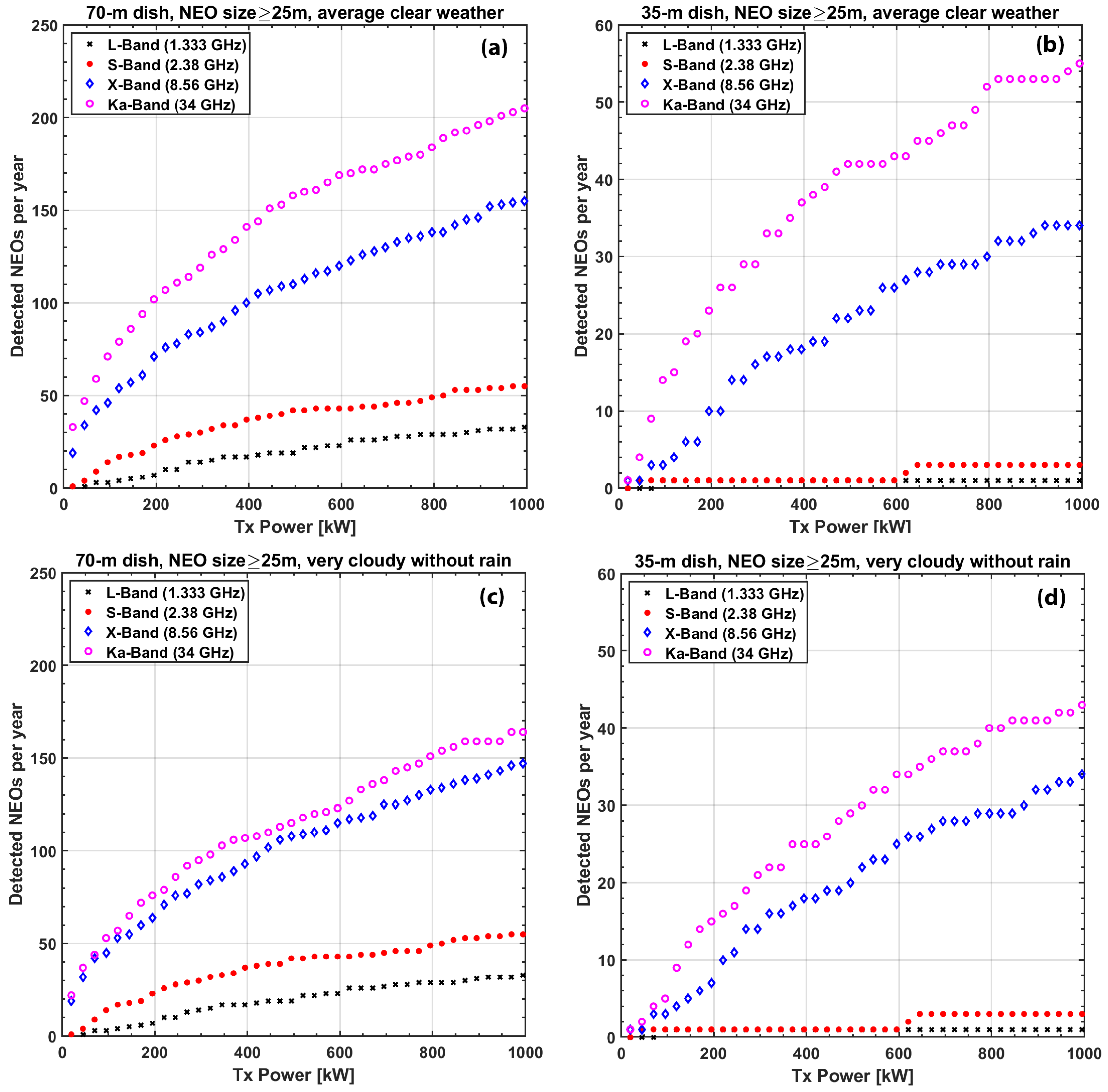We considered different frequency bands, including the historically employed ones (L at TIRA, S at Arecibo, and X at Goldstone), and the possibility of operating at higher frequencies, particularly in the Ka-band (∼34 GHz), which has been hypothesized for the Green Bank Telescope (GBT) [16]. We estimated the number of detectable NEOs per year—whose echo would exceed a given Signal-to-Noise Ratio (SNR) value (the choice of an SNR threshold value of 30/track will be discussed later)—as a function of the transmitted power, for four different transmitted frequencies: L (1.333 GHz), S (2.38 GHz), X (8.56 GHz), and Ka (34.0 GHz), corresponding to existing radar systems or taken into account for the possible design of future planetary radar instruments. The technical parameters were inspired by the ones characterizing real antennas, when such examples were available in the various bands; otherwise, plausible values were derived/rescaled according to the literature. In

Table 1. Key parameters for simulated sensors.

Tx Band and Frequency (GHz)	Antenna Diameter (m)	${\mathit{T}}_{\mathbf{AMW}}$ (K)	Gain (dBi)
L (1.333)	35	26.68	53.08
S (2.38)	35	18.27	57.90
X (8.56)	35	11.46	68.00
Ka (34.0)	35	19.57	79.77
L (1.333)	70	26.68	59.10
S (2.38)	70	18.27	63.92
X (8.56)	70	11.46	74.02
Ka (34.0)	70	19.57	85.79

are listed the main parameters of the sensors used in the simulations: radio frequency band with the operating frequency, antenna size, noise temperature $T_{AMW}$ due to the antenna and its microwave components (without atmosphere noise temperature), and antenna gain. Here, the antenna gain is expressed in dBi: $G_{dBi}=10{log}_{10}\left(4\pi \eta A_{ant}/{\lambda }^2\right)$, where $\eta$ is the antenna aperture efficiency, $A_{ant}$ is the geometric area of the antenna, and $\lambda$ is the radar wavelength.

A standard atmospheric model [17] was applied to estimate the atmospheric attenuation and noise temperature at the considered frequencies in four weather scenarios. Such weather profiles were derived from statistics measured at the MDSCC [18]. As potential targets, we used the list of NEOs that had a close approach to Earth in the solar year 2020 at a distance ≤ 0.2 astronomical units (au) (divided into three size categories: all, ≥25 m, and ≥140 m) and that were in the visibility window (target elevation $\ge {20}^{°}$) of a radar located at the Madrid DSN site.

The SNR of the radar echo was estimated at the time of close approach (TCA), i.e., when the object was at its minimum distance from Earth, using Equation (1).

$$SNR=\frac{P_T{G}_T{G}_R{\lambda }^{\frac{5}{2}}}{512{\pi }^{\frac{5}{2}}k{T}_{sys}}·\frac{\widehat{\sigma }{D}^{\frac{3}{2}}{P}^{\frac{1}{2}}}{R_T^2{R}_R^2}·{(\Delta t)}^{\frac{1}{2}}$$

(1)

where $P_T$ is the transmitted power, $G_T$ and $G_R$ the gain of the transmitting and the receiving antennas, respectively, $\lambda$ the signal wavelength, $\widehat{\sigma }$ the target radar albedo, D the target diameter (which was assumed to have a spherical shape), P the target rotational period, $\Delta t$ the signal integration time, k the Boltzmann constant, $T_{sys}$ the receiver system temperature, and $R_T$ and $R_R$ the range from the target to the transmitter and from the target to the receiver, respectively. In the specific case of monostatic observations, since the receiving and the transmitting antennas are the same, we have $G_T=G_R$ and $R_T=R_R$.

It was derived from the radar equation for a bistatic configuration, with the assumption that the mean level of the receiver noise power is stable and removed as background, and the bandwidth is equal to the intrinsic echo width in the case of an equatorial view of the target [19]. The assumed bandwidth, B (Hz), for each target was calculated by Equation (2) [5]:

$$B=\frac{4\pi Dcos\left(\delta \right)}{\lambda P}$$

(2)

where P is the target rotation period (s), $\lambda$ is the signal wavelength (m), D is the target projected diameter (m), and $\delta$ is the subradar latitude (angle between the radar line-of-sight and the object rotational equator), here assumed as $\delta =0^{°}$.

In our simulations, when a target parameter was unknown, we assumed: a typical radar albedo value $\widehat{\sigma }=0.1$ [20], a target spin period $P=2.1$ h if $D\ge 140$ m and $P=0.5$ h for smaller objects [9], and finally, a target diameter D derived from its absolute magnitude (H) assuming an optical albedo of 0.14 as in the ESA Near-Earth Object Coordination Center (NEOCC) database [21].

An SNR threshold value of ≥30/track was adopted, as above this SNR threshold, the rate of successful detection is close to 100% and accurate astrometry measurements can be performed [9]. A “readiness threshold” was also applied, to take into account a real-world scenario: targets with a discovery date closer than 5 days to their visibility window were discarded.

Figure 1 shows the expected yearly detections with an SNR ≥ 30 of asteroids larger than 25 m, if employing a 70 m and a 35 m dish, both in monostatic radar configuration under weather conditions defined as “average clear weather” (CD = 0.25) and “very cloudy without rain” (CD = 0.90). The CD value represents the statistics’ cumulative distribution of the described atmospheric conditions. For example, CD = 0.90 means that 90% of the days (on a yearly basis) have atmospheric attenuation and a noise temperature equal to or better (i.e., lower) than the ones associated with the descriptive label. It must be stressed that monostatic systems, though more easily manageable, reduce the observation efficiency by about 50%, as transmission and reception take place alternatively. This means that, when longer integration times are needed, multistatic observations are more effective. These results clearly showed how, given a certain transmitted power, a transmitter in the Ka-band is more productive than lower-frequency ones, even under a usually cloudy sky. Ka-band transmitters roughly need half the power required to reach a given performance in the X-band. This advantage depends on the greater directivity at higher frequencies. Conversely, it must be noticed that, at such high power levels, X-band transmitters are presently the most-used and better characterized, while Ka-band ones suffer from limitations—such as significant losses in the waveguides, not considered in our simulations. In comparison, the L-band and S-band choices—though weather-invariant—grant a much lower rate of successful observations, especially for dishes in the 35 m class, as their lower sensitivity further significantly reduces the number of possible detections. A comprehensive description and detailed results of these simulations will be presented in a forthcoming publication.

3. Facilities

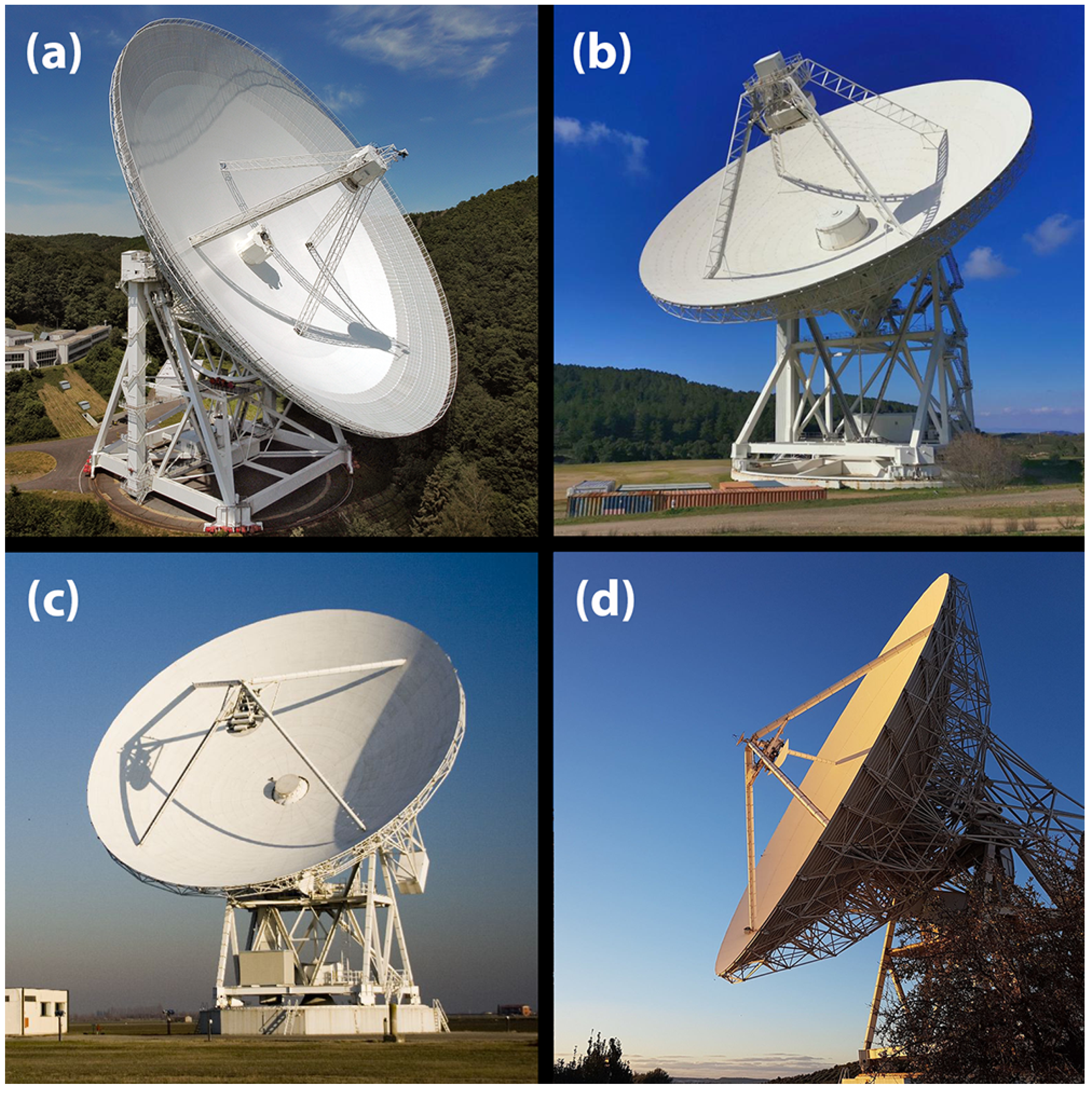
Considering both the availability and the compatibility of receivers with the transmitted frequencies, for the radar observations, the Effelsberg, Medicina, Noto, and Sardinia Radio Telescope (SRT) antennas (see Figure 2) were selected as receivers.

The Effelsberg radio telescope is a 100 m dish operated by the Max-Planck-Institut für Radioastronomie (MPIfR) and is located in a valley, for protection against Radio Frequency Interferences (RFIs), near Bad Münstereifel-Effelsberg, Germany. It is one of the two largest fully steerable single-dish radio telescopes in the world and a unique high-frequency radio telescope in Europe. The telescope can be used to observe radio emissions from celestial objects in a wavelength range from 90 cm (300 MHz) down to 3.5 mm (90 GHz).

Medicina, Noto, and SRT are facilities managed by INAF. The one in Medicina (Grueff Radio Telescope) is a 32 m parabolic dish located inside the Medicina radio observatory, 30 km from Bologna, Italy. The antenna is provided several receivers in the 1.4–26.5 GHz range and is employed for both interferometric and single-dish observations. In the very near future, its primary mirror will be upgraded to an active surface, allowing it to increase the overall efficiency at higher frequencies and perform observations with stable gain at all elevations. The Noto radio telescope, located in the southern part of Sicily (Italy), is a 32 m antenna with an active surface, mainly focused on geodynamic, galactic, and extragalactic research. Finally, the SRT, located in the southern part of the island of Sardinia (Italy), is the largest Italian parabolic dish with a 64 m diameter and one of the most-advanced radio telescopes in the world. The SRT is co-managed by the Italian Space Agency (ASI), named the Sardinia Deep Space Antenna (SDSA) due its activities, and is equipped with an X-band receiver for deep space and Near-Earth activities [22]. In 2024, all three Italian radio telescopes will be equipped with new tri-band K-Q-W receivers capable of acquiring simultaneously the frequency bands 18–26, 33–50, and 80–116 GHz [23].

Table 2. Main features of the receiving antennas.

	Effelsberg	SRT/SDSA	Medicina	Noto
Longitude	${06}^{°}{53}^{\prime }{01.0}^{″}$ E	${09}^{°}{14}^{\prime }{42.5}^{″}$ E	${11}^{°}{38}^{\prime }{49.0}^{″}$ E	${14}^{°}{59}^{\prime }{20.6}^{″}$ E
Latitude	${50}^{°}{31}^{\prime }{29.4}^{″}$ N	${39}^{°}{29}^{\prime }{30.0}^{″}$ N	${44}^{°}{31}^{\prime }{13.8}^{″}$ N	${36}^{°}{52}^{\prime }{33.8}^{″}$ N
Diameter	100 m	64 m	32 m	32 m
Rx bands	L, C, X, Ku, K, Ka	P, L, C, X, K	L, S, C, X, K	L, S, C, X, K
Decl. range	$-31.4^{°}$ to $+{90}^{°}$	$-44.5^{°}$ to $+{90}^{°}$	$-40.5^{°}$ to $+{90}^{°}$	$-48.1^{°}$ to $+{90}^{°}$
Min. elev.	$8.1^{°}$	$6^{°}$	$5^{°}$	$5^{°}$
Max. elev.	${89}^{°}$	${82}^{°}$	${88}^{°}$	${88}^{°}$
Max. speed	$0.5^{°}$/s Az.; $0.{27}^{°}$/s El.	$0.{85}^{°}$/s Az.; $0.5^{°}$/s El.	$0.8^{°}$/s Az.; $0.5^{°}$/s El.	$0.8^{°}$/s Az.; $0.5^{°}$/s El.
Pointing accuracy (rms)	$0.{003}^{°}$	$0.{001}^{°}$	$0.{002}^{°}$	$0.{002}^{°}$
Active mirror	yes	yes	imminent	yes

summarizes the main general features of the receiving antennas. Technical details for the Effelsberg and the INAF antennas can be found in [24] and [25], respectively.

Since all those radio telescopes are elements of the European Very Long Baseline Interferometry Network (EVN), they are equipped with atomic clocks for synchronization and employ the same Digital Baseband Converter (DBBC) backend for data acquisition [26]. Having the DBBC installed on multiple antennas offers the advantage of standardizing the observation procedure and generating uniform data formats as the output. The output of the DBBC is the VLBI Data Interchange Format (VDIF), which is the common raw-data format to all Very Long Interferometry (VLBI) antennas [27], even those that install other backends. This facilitates the development and use of common software for data processing.

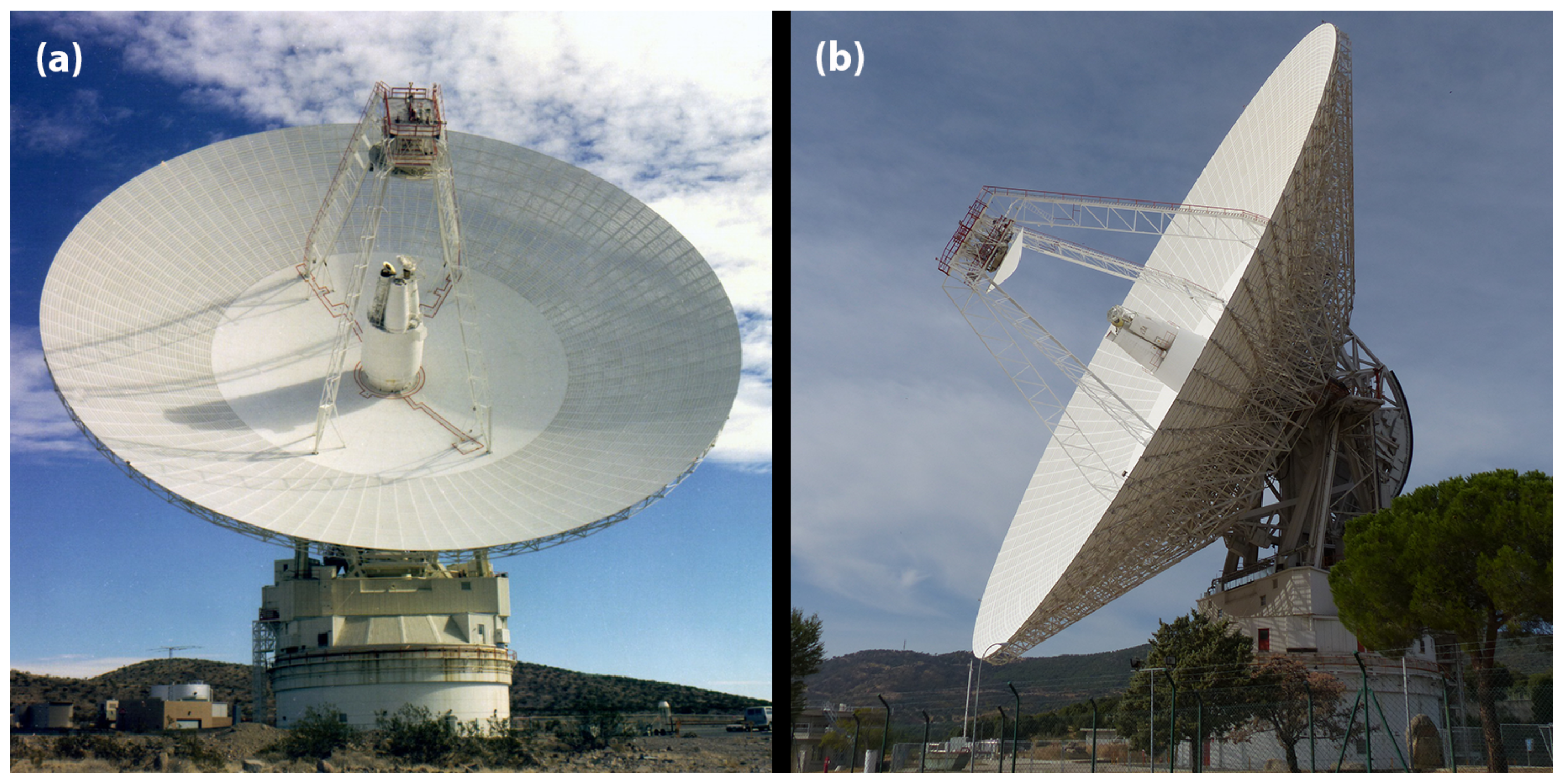
For the transmitting part, after the collapse of Arecibo, the choice fell necessarily on the 70 m DSS-14 and DSS-63 antennas (see Figure 3) belonging to the DSN.

The DSS-14 is operated by NASA/JPL and is located near Barstow, in the Mojave Desert, California. In addition to the DSN communication system, DSS-14 is also equipped with a planetary radar, capable of transmitting with a power of 450 kW at a 3.5 cm wavelength (X-band). The DSS-14 is currently the main operational ground-based planetary radar, named the Goldstone Solar System Radar (GSSR), significantly employed for the observation of NEOs [28,29]: it observes NEOs for about 20% of its operational time. Also, the DSS-43 in Canberra has been performing, since 2015, planetary radar activities [30]. The DSS-63 is located at the Madrid Deep Space Communications Complex owned by NASA/JPL, just outside of Madrid (Spain), in Robledo de Chavela. It currently installs the standard 20 kW DSN transmitters operating in the S- and X-band. DSS-63 took part, as a receiver, in the radar observations of Golevka in June 1999 [31], when Arecibo was the transmitting antenna. The DSS-63 was first employed for transmission in a NEO experiment during our observations of 2005 LW3, making it the first fully European NEO radar campaign after the Evpatoria dish became unavailable. The main characteristics of the transmitting dishes are summarized in

Table 3. Main features of the transmitting antennas.

	DSS-14 (Goldstone) 1	DSS-63 (Madrid)
Longitude	${243}^{°}{06}^{\prime }{37.8}^{″}$ E	${355}^{°}{45}^{\prime }{07.2}^{″}$ E
Latitude	${35}^{°}{25}^{\prime }{33.2}^{″}$ N	${40}^{°}{25}^{\prime }{52.4}^{″}$ N
Diameter	70 m	70 m
Tx bands	X	S, X
Tx Power	450 kW	20 kW
Decl. range	$-34.6^{°}$ to $+{90}^{°}$	$-29.6^{°}$ to $+{90}^{°}$
Min. elev.	${20}^{°}$	${20}^{°}$
Max. elev.	${89}^{°}$	${89}^{°}$
Max. speed	$0.{25}^{°}$/s	$0.{25}^{°}$/s
Pointing accuracy (rms)	$0.{005}^{°}$	$0.{005}^{°}$

¹ In planetary radar configuration.

.

4. Definition of Observing Campaigns: Selection of Targets and Facilities

The definition of the observing campaign started by consulting the list of known close approaches, considering those foreseen in the time frame of interest. The source for this information was the NEODyS database [32]. The total number of known NEOs as of 1 January 2021, with a close approach to Earth during the same year at a distance < 0.2 au, was 1066. This list has been continuously updated with close approach events of the new objects discovered after 1 January 2021. In parallel, and iteratively, the suitability and availability of the transmitting and receiving antennas were ascertained, to identify the actual exploitable combinations and check the performance they could achieve on the different potential targets. We searched for asteroids for which a common Tx–Rx visibility window was available and whose SNR estimates, obtained using the software tools we developed, were suitable at least for detection. As the actual feasibility of an experiment also depends on the absence of strong RFI in the observed band, it was necessary to verify that no major issues were present at the Rx facility. The overall scheme of the activities, from the initial campaign definition to the results produced after data processing, is presented in Figure 4. Image processing is a forthcoming activity, also thanks to the presence of expert staff in our collaboration.

A comprehensive list of the experiments executed within the framework of the ESA project is provided in

Table 4. List of the executed experiments. MC = Medicina, NT = Noto, SDSA = Sardinia Deep Space Antenna, EF = Effelsberg.

Date	Target	Tx	Rx	Result
3 May 2021	2021 AF8	DSS-14	SDSA, MC	Detected SDSA
23 Aug 2021	2016 AJ193	DSS-14	MC	Detected
10, 15 Dec 2021	(4660) Nereus	DSS-14	MC	Detected
28 Apr 2022	2008 AG33	DSS-63	EF	Not detected
25 May 2022	1989 JA	DSS-63	EF	Not detected
23 Nov 2022	2005 LW3	DSS-63	MC, EF	Detected at both
15 Dec 2022	2015 RN35	DSS-63	MC, NT, EF	Not detected
27 Dec 2022	2010 XC15	DSS-63	MC	Detected

. It is worth noticing that the Italian radio telescopes have successfully taken part in radar experiments on NEOs since 2001 [33].

5. Observations

In this section, we describe three radar experiments conducted during and after the ESA project. These experiments were chosen as representative examples of observations carried out using different radar systems and data-processing techniques. Data reduction and analysis were performed using software tools we specifically developed in Python (version 3.8.8) and Matlab (R2021b)

5.1. 2021 AF8

Asteroid 2021 AF8 was discovered by the Mt. Lemmon Survey, part of the Catalina Sky Survey (CSS) Program, on 2021 January 14 [34]. The object (see

Table 5. Orbital and physical properties of 2021 AF8, as they were known before radar observations.

Target	2021 AF8
Epoch (MJD)	60,200.0
Orbit type	Apollo
Eccentricity	0.517
Inclination (deg)	9.7
Perihelion distance (au)	0.973
Aphelion distance (au)	3.058
Orbital period (days)	1045.3
Close approach distance (au)	0.022
Close approach date (UT)	12:12 4 May 2021
Earth MOID (au)	0.02783
Absolute magnitude (H)	20.2
Diameter (m)	∼300
Rotation period (h)	unknown
Optical albedo	unknown
Radar albedo	unknown
Spectral class	unknown

) is classified as a Potentially Hazardous Asteroid (PHA) by the International Astronomical Union’s Minor Planet Center. Before radar observations, neither the size, nor the rotation period of this target were known. The size had been estimated from its absolute magnitude, assuming a mean optical albedo of 0.14 [21].

Our radar observations of 2021 AF8 were carried out on 3 May 2021. They produced interesting results, thanks to the high sensitivity of the employed system, which involved the DSS-14 (Goldstone) for transmission and the SRT/SDSA on the receiving side.

Table 6. System parameters for the observation of 2021 AF8.

	Transmitter	Receiver
	DSS-14	SRT/SDSA
Diameter	70 m	64 m
Aperture Efficiency	0.64	0.54
Tx Frequency	8560 MHz	-
Tx Power	450 kW	-
Tx Waveform	CW	-
System Temperature	-	42 K
Polarization	RCP	LCP

summarizes the main system parameters.

The DSS-14 scheduled radar observations of 2021 AF8 in monostatic configuration for 3 May 2021 from 15:05 UT to about 17:05 UT. JPL agreed to allow the recording of the echo signal during their observations (“eavesdropping”) and provided details on the transmission configuration type and timing (start/stop). Since this DSS-14 campaign was designed for a monostatic radar configuration:

• The frequency of the transmitted signal was modified in order to compensate for the Doppler variations—due to the known motion of the target (from ephemerides, dynamic compensation)—relative to the transmitting antenna DSS-14 only. A signal received at any other location would show a frequency drift;
• The observation needed to be divided into transmission/reception cycles (runs). Each run consisted of signal transmission for a duration close to the round-trip light time (RTT) between the radar and the target, followed by a reception for a similar duration. An additional 5 s, due to the transmission–reception switch time, contributed to the overall run duration [9].

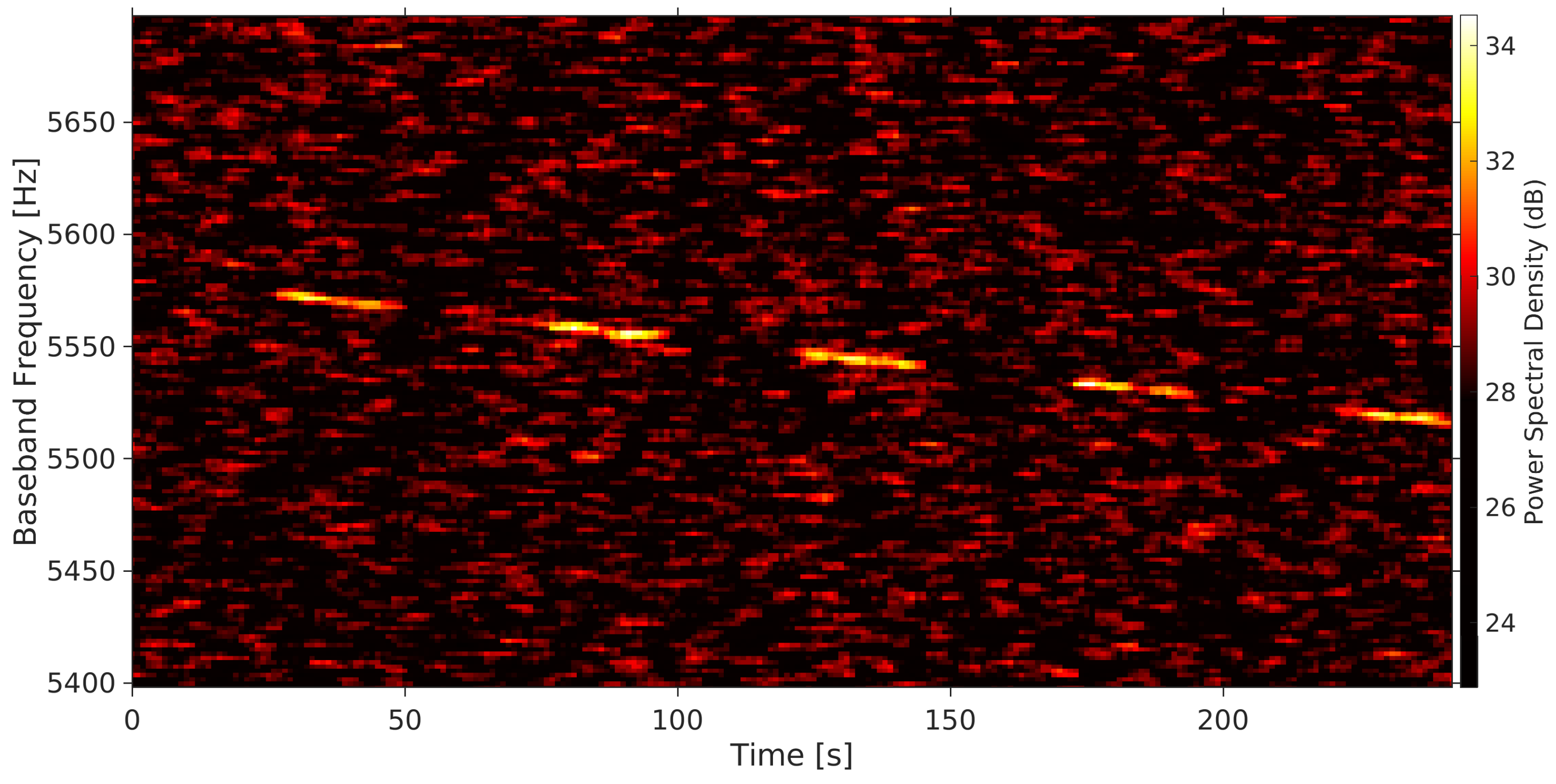
Both the Doppler frequency drift, due to the displacement of our antenna with respect to the intended receiver, and the transmission on/off runs of about 28 s duration were evident in the spectrogram of the received signal recorded at the SRT/SDSA without Doppler compensation (Figure 5). To produce the power spectra, we employed the Discrete Fourier Transform (DFT) and the Welch power spectral density (PSD) estimator [35]. This method, also known as Welch’s overlapped segment averaging (WOSA), divides the time signals into partially overlapping windowed segments, to avoid signal loss. Such data processing with an overlap fraction of 0.5 yielded a ∼30% improvement of the SNRs with respect to the standard processing without overlapping [36]. Another typically used overlap fraction value, to achieve high accuracy in the PSD estimation, is 0.75 [37], which was the value applied in our analysis. The chosen integration time in the spectrograms without Doppler compensation was a trade-off between increasing the SNR and minimizing the intra-spectrum frequency smearing.

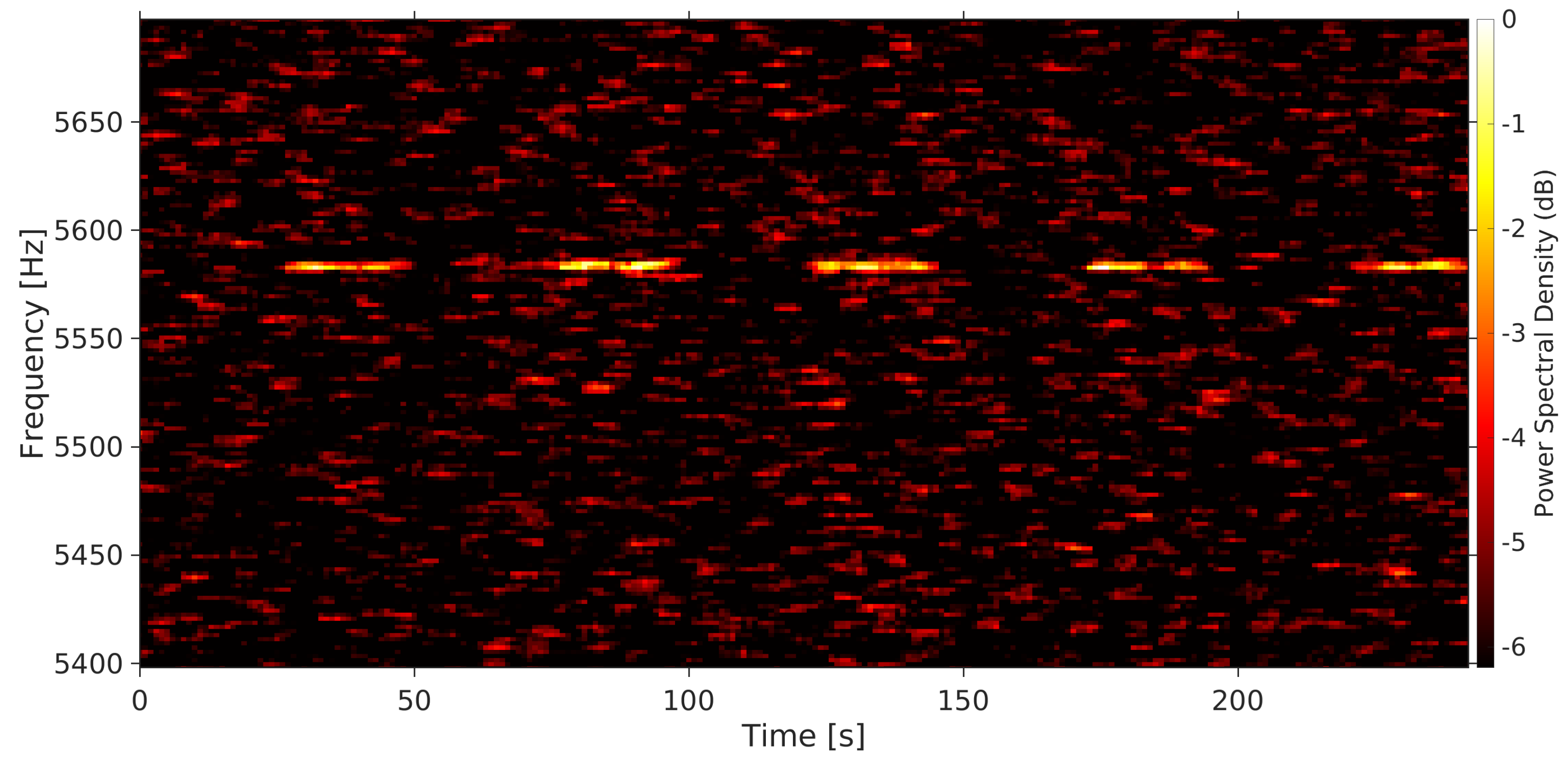
The spectral smearing, due to the frequency drift, limits the maximum spectral resolution that can be achieved in the Doppler analysis and reduces the SNR. To remove the frequency drift, a Doppler compensation was, thus, performed by using the phase-stopping technique [38,39]. It consisted of:

• Calculating the polynomial fit of the echo frequency $F\left(t\right)$ as a function of time;
• Deriving the phase polynomial fit, the coefficients of which were obtained by integrating those of $F\left(t\right)$;
• Multiplying each raw sample acquired in the time domain by the corresponding complex-valued phase correction derived from the phase polynomial fit.

A detailed description of this method and its implementation was given in [40]. We modeled the frequency variation using a third-order weighted least-mean-squares (WLMS) polynomial fit of those spectrum peaks exceeding an SNR = 10. The weights are the SNR values.

The successful removal of the frequency drift is evident in the spectrogram of the 2021 AF8 signal (Figure 6) obtained from the time domain data after the Doppler compensation.

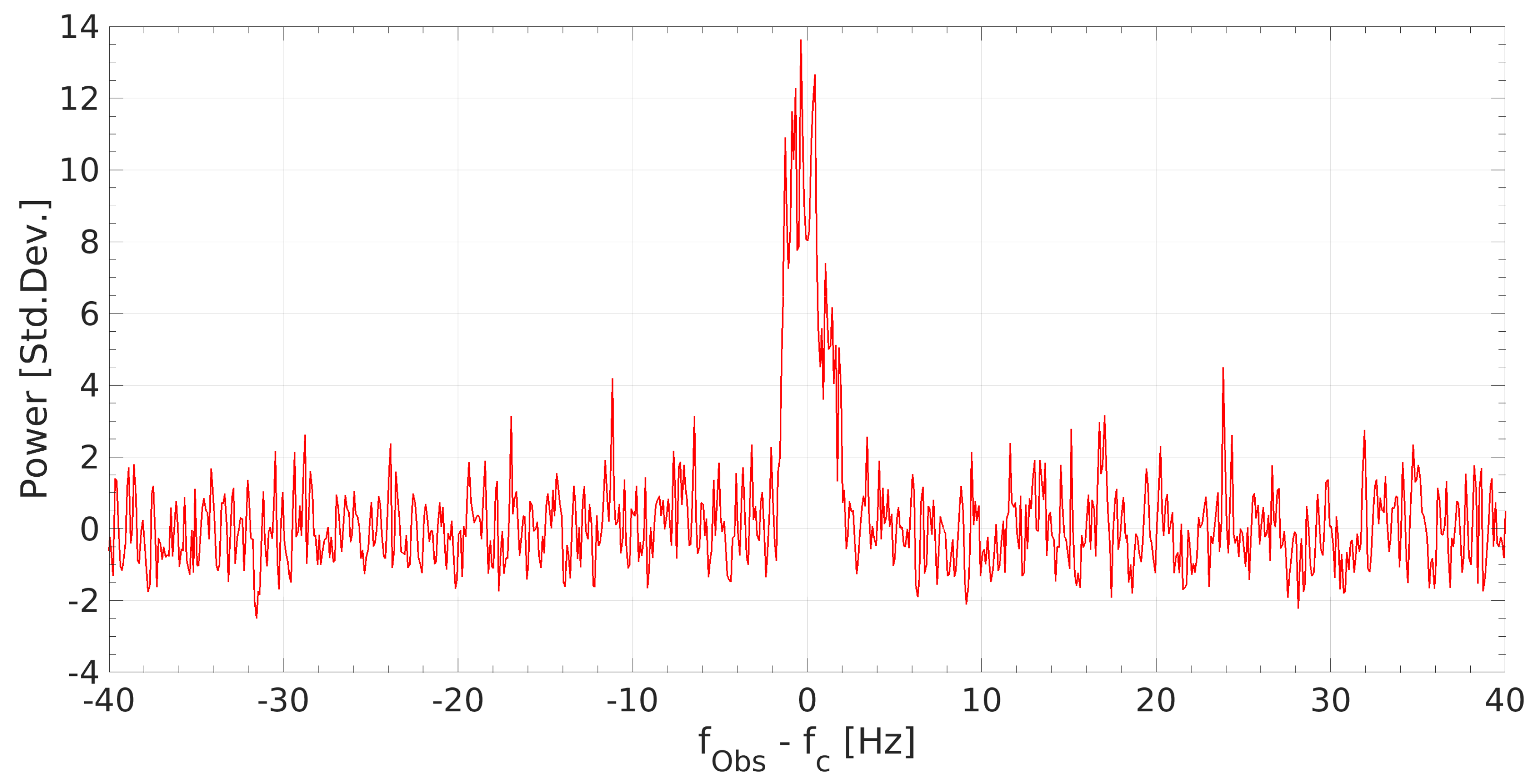
Data corrected for Doppler drift allowed the production of high-resolution (sub-Hz) integrated power spectra (see Figure 7) because they were no longer affected by frequency smearing. The integration was performed only on the five time intervals containing the signal for a total of an ∼100 s integration time.

In each integrated spectrum, the mean noise background (baseline) was estimated with a fifth-degree polynomial fit considering two spectral regions adjacent to the radar echo. This baseline was subtracted from the spectrum, and the residual was divided by the noise standard deviation of the baseline. This standard post-processing procedure was employed for all targets.

In this plot, the frequencies are expressed as the difference between the received frequency $f_{Obs}$ and that of the echo spectral centroid $f_c$ = 8,559,982,136.1 Hz, estimated from:

$$f_c=\frac{{\sum }_{i=n_{-}}^{n_{+}}{f}_i{m}_i}{{\sum }_{i=n_{-}}^{n_{+}}{m}_i}$$

(3)

where $n_{-}$ and $n_{+}$ are the number of frequency bins corresponding to the left and right edge of the echo, respectively. $f_i$ is the central frequency of the i-th frequency bin and $m_i$ the echo power in that bin.

The echo of the asteroid was well resolved in the high-resolution spectra. This allowed us to exploit the inverse of Equation (2) to estimate the asteroid rotation period.

The echo broadening was estimated as the limb-to-limb width of the radar echo profile at zero-sigma crossing. This is a common threshold used in echo width estimation (e.g., [7]), although other standards exist such as the two-sigma crossing (e.g., [41]). Our measurements of the Doppler broadening yielded a rough estimate of the 2021 AF8 rotation period of ∼7.7 h, considering an equatorial view ($\delta =0^{°}$). The subradar latitude is unknown; therefore—under our assumption—the value obtained is an upper limit of the effective target rotation period. The only other available measurement, obtained with a lower-frequency resolution (1 Hz) and a lower SNR than ours, is provided by the Institute of Applied Astronomy of the Russian Academy of Sciences (IAA RAS): the rotational period is stated to be approximately 6 h [42].

Since the SDSA receiver was capable of acquiring only one circular polarization at a time, it was not possible to perform a polarization analysis of the signal in this experiment.

5.2. (4660) Nereus

Asteroid (4660) Nereus was discovered in February 1982 by E.F. Helin using the 18${}^{″}$ Schmidt telescope at Palomar Mountain Observatory [43]. Its orbital and physical properties are listed in

Table 7. Orbital and physical properties of (4660) Nereus.

Target	(4660) Nereus
Epoch (MJD)	60,200.0
Orbit type	Apollo
Eccentricity	0.359
Inclination (deg)	1.5
Perihelion distance (au)	0.953
Aphelion distance (au)	2.018
Orbital period (days)	661.1
Close approach distance (au)	0.026
Close approach date (UT)	13:50 11 December 2021
Earth MOID (au)	0.00426
Absolute magnitude (H)	18.7
Diameter (m)	510 × 330 × 240
Rotation period (h)	15.16
Optical albedo	0.39
Radar albedo	0.44
Spectral class	X

. Some of the physical properties were studied during the close approach in 2002. This object is elongated with an effective diameter of 330 m and is a member of the optically bright E-spectral-class asteroids. Nereus approached within 0.0263 au on 11 December 2021, and it was a strong radar target for several weeks.

During the period 10–15 December 2021, the Goldstone DSS-14 scheduled the observation of Nereus in Speckle interferometry mode [44], in which the Very Long Baseline Array (VLBA) was the receiving part. In agreement with L. Benner and M. Brozovic at JPL, Medicina joined the experiment in eavesdropping, in the following time intervals:

• 10 December 2021, 12:44:25–13:05:15 UT;
• 15 December 2021, 12:20:00–12:40:00 UT.

The main system parameters for the observation of Nereus with the DSS-14 and Medicina are provided in

Table 8. System parameters for the observation of (4660) Nereus.

	Transmitter	Receiver
	DSS-14	Medicina
Diameter	70 m	32 m
Aperture Efficiency	0.64	0.48
Tx Frequency	8560 MHz	-
Tx Power	450 kW	-
Tx Waveform	CW	-
System Temperature	-	38 K
Polarization	RCP	RCP, LCP

.

In the radar Speckle experiments, similar to a standard bistatic observation, CW transmission was employed without interruptions, but the Doppler was compensated for the Earth center—and not for a specific antenna. This led to a residual Doppler shift in the received signal, which we removed in post-processing through the phase-stopping method. 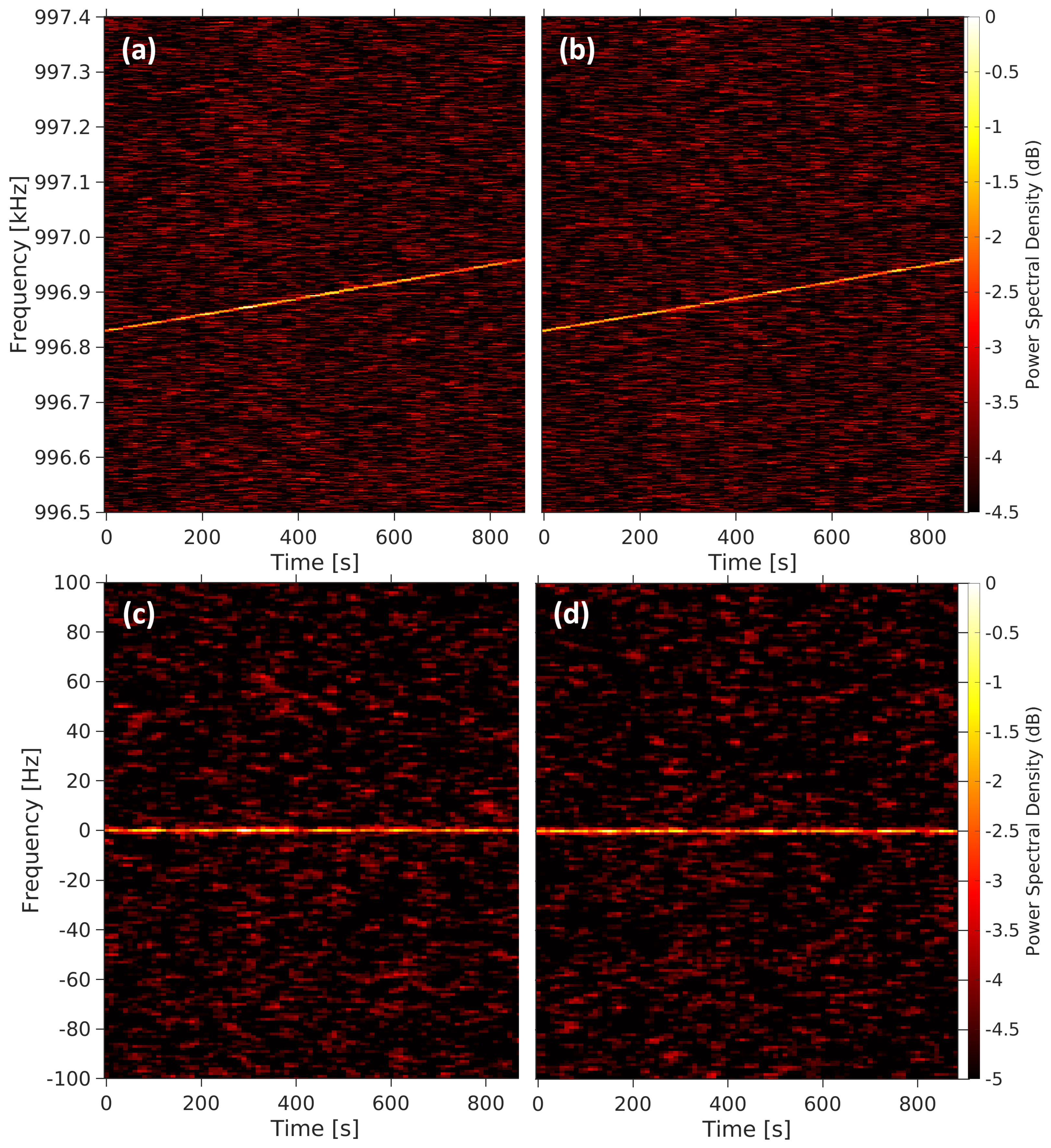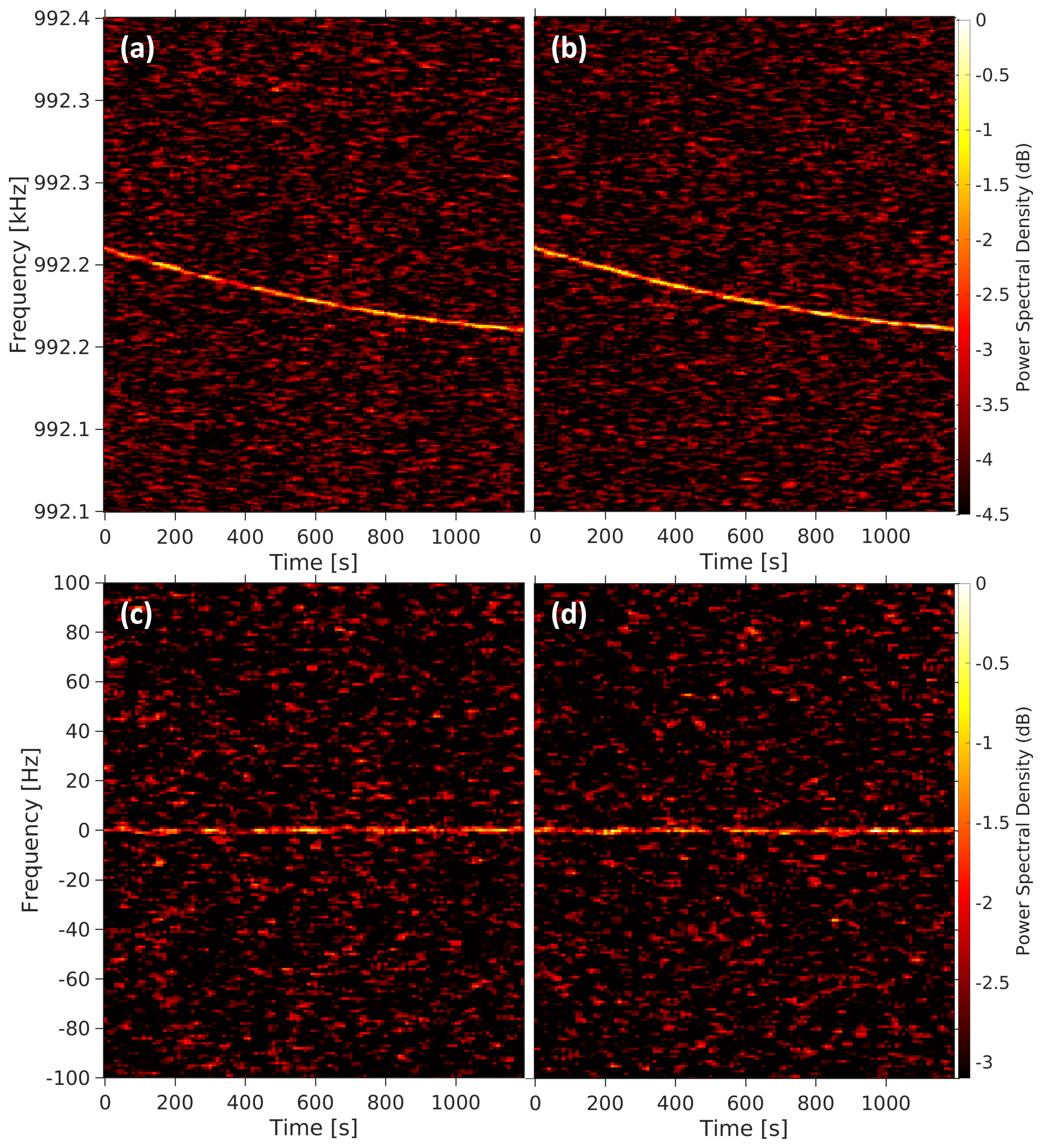Unlike the case of 2021 AF8, here, the phase polynomial coefficients were calculated from the ephemeris-based predictions provided by SpaceDyS, according to the method described in [38,39]. Spectrograms of the Nereus echo in both Left Circular Polarization (LCP) and Right Circular Polarization (RCP), both with and without the Doppler compensation, are shown in Figure 8 and Figure 9, respectively, for 10 and 15 December 2021.

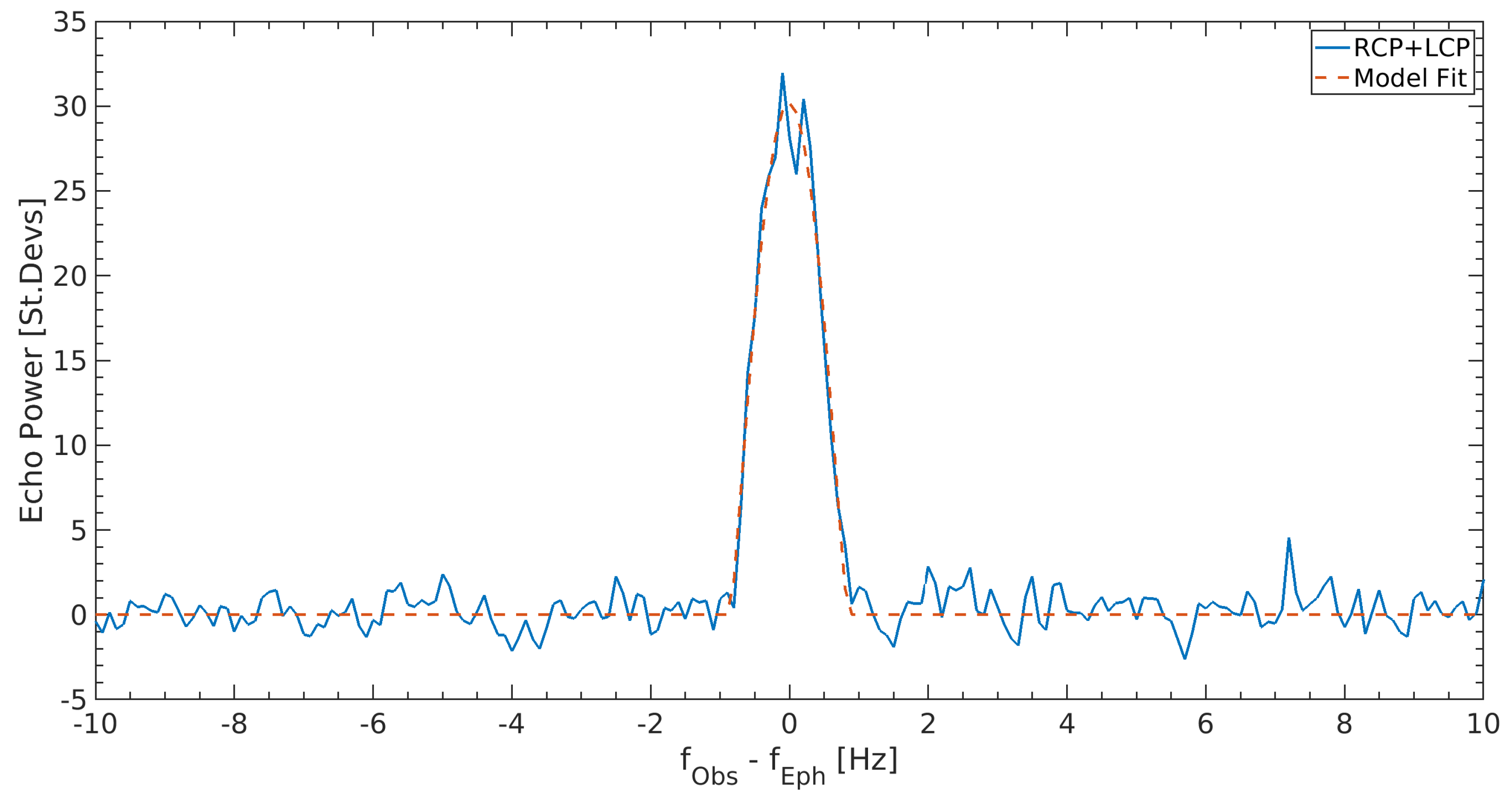
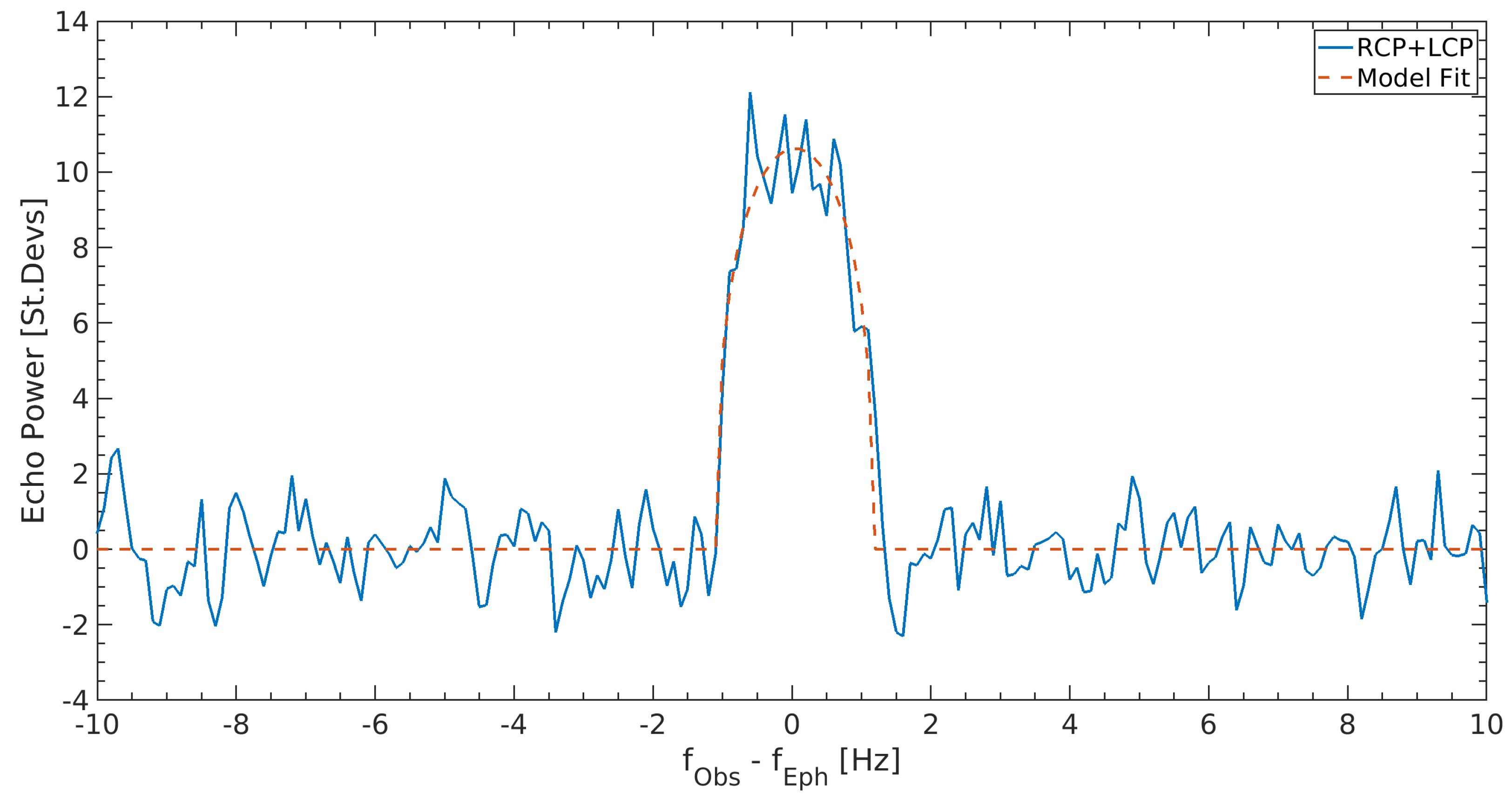
High-resolution power spectra at 0.1 Hz (see Figure 10 and Figure 11) allowed us to measure both the frequency at the center of mass (COM) for astrometry computations and the asteroid rotation period. To increase the SNR further, each integrated spectrum was the combination of the power spectra acquired in RCP and LCP. In the estimate of the echo broadening, besides the usual limb-to-limb Doppler bandwidth method, we employed also a multi-parametric fitting with a simple echo profile model [45]. This method consisted of accurately removing the noise baseline and, then, expressing the signal in terms of standard deviation units of the background noise, fitting with a least-squares method the linear baseline and a signal profile model defined by four parameters: echo width and amplitude, peak position, and shape parameter. Both estimation methods yielded similar results.

On both days of observation, the measurements gave a practically nil difference (within the uncertainties) between the observed COM frequency and that predicted by the ephemeris, testifying to the goodness of both the ephemeris solutions used and the Doppler compensation procedure performed on the time domain data. As concerns the echo bandwidth, the measurements yielded: $B=1.7\pm 0.1$ Hz for 10 December and $B=2.3\pm 0.2$ Hz for 15 December. The associated uncertainty was calculated as the maximum between the spectral resolution and the standard error in the model fit.

Nereus had already been characterized through radar observations carried out at Goldstone and Arecibo during the previous close approach in 2002 [46]. They measured the rotation period $P=15.16\pm 0.04$ h with high accuracy and located approximately the pole direction at $\lambda =+{25}^{°}$, $\beta =+{80}^{°}$ ecliptic coordinates, albeit with an uncertainty of $\pm {10}^{°}$.

From the pole direction coordinates, we calculated the subradar latitude $\delta$ at the time of the observation. Since the rotation period of Nereus is known, we exploited the inverse of Equation (2) to derive the breadth D of the asteroid polar silhouette projected on the plane-of-sky from our instantaneous echo bandwidth measurements. The obtained values of the projected size D of Nereus at the time of observation are listed in the last column of

Table 9. Measurements of the Nereus projected diameter.

Observation Date	$\mathit{\delta }$	B	D
(UT)	(deg)	(Hz)	(m)
10.538 December 2021	$\delta =+{47}_{-7}^{+3}$	$1.7\pm 0.1$	$379\pm 54$
15.521 December 2021	$\delta =+{29}_{-10}^{+9}$	$2.3\pm 0.2$	$400\pm 73$

.

These measurements are consistent with the principal axis dimensions of Nereus (510 m × 330 m × 241 m) derived from the delay-Doppler images acquired at Goldstone and Arecibo during the 2002 radar campaigns [46].

In observations such as those of Nereus, in which the echo is detected in both circular polarizations, it is possible to calculate the circular polarization ratio ${\mu }_c$, defined as:

$${\mu }_c=SC/OC$$

(4)

where SC is the received echo power in the same polarization sense as transmitted (here, RCP) and OC that in the opposite sense (here, LCP). The polarization ratio is one of the most-important physical observables in the NEO radar technique, as it provides information about the asteroid’s surface and sub-surface roughness/complexity at the wavelength scale [47].

A preliminary analysis of our spectra indicated a high value of the polarization ratio, typical of the E-class-spectral-type asteroids such as Nereus. Our rough estimate was close to 1. This value is not fully in agreement with the previous measurements performed at Goldstone and Arecibo, which reported a value of $0.74\pm 0.08$ [46]. It must be said that an accurate evaluation of this ratio from our measurements will be possible only once a proper polarization calibration procedure is implemented.

5.3. 2005 LW3

The asteroid 2005 LW3 was discovered on 5 June 2005 with the 0.5 m Uppsala Southern Schmidt Telescope (Australia) in the framework of the Siding Spring Survey (SSS) [48], which is the counterpart in the Southern Hemisphere of the CSS. This asteroid has an absolute magnitude (H) of 21.7, which suggested, before the radar observations, a diameter of about 160 m (see

Table 10. Orbital and physical properties of 2005 LW3, as they were known pre-radar observations.

Target	2005 LW3
Epoch (MJD)	60,200.0
Orbit type	Apollo
Eccentricity	0.464
Inclination (deg)	6.0
Perihelion distance (au)	0.772
Aphelion distance (au)	2.106
Orbital period (days)	630.3
Close approach distance (au)	0.0076
Close approach date (UT)	10:05 23 November 2022
Earth MOID (au)	0.00134
Absolute magnitude (H)	21.6
Diameter (m)	∼170
Rotation period (h)	unknown
Optical albedo	unknown
Radar albedo	unknown
Spectral class	unknown

). Nothing else was known about the asteroid’s physical properties.

Thanks to JPL/DSN, we carried out the observation of this object on 23 November 2022, using the DSS-63 antenna in Madrid as the transmitter in a multistatic radar configuration, with the Effelsberg and Medicina antennas as receivers.

Table 11. System parameters for the observation of 2005 LW3.

	Transmitter	Receiver 1	Receiver 2
	DSS-63	Effelsberg	Medicina
Diameter	70 m	100 m	32 m
Aperture Efficiency	0.70	0.55	0.52
Tx Frequency	7167 MHz	-	-
Tx Power	20 kW	-	-
Tx Waveform	CW	-	-
System Temperature	-	30–40 K	90 K
Polarization	RCP	LVP, LHP	RCP, LCP

shows the main parameters of the radar system employed in our experiment. Despite the limited power available at the DSS-63 facility (20 kW), the possibility to exploit the large Effelsberg radio telescope on the receiving side, together with the Medicina 32 m antenna, permitted us to achieve a suitable SNR and accuracy in the measurements.

Transmission at a fixed frequency of 7167 MHz was agreed with JPL so that the echoes were received at Medicina in a spectral region free from impacting RFIs. The DSS-63 transmitted the CW signal for approximately 3.17 h, starting from 15:50 to 19:00 UT on 23 November 2022, with some short interruptions for satellite avoidance.

Note that the signal transmitted by the DSS-63 was in RCP, whereas the receiver used at Effelsberg acquired Linear Vertical Polarization (LVP) and Linear Horizontal Polarization (LHP) signals. Consequently, half of the power of the incoming signal was recorded by each received linear polarization. In this case, the measurement of the polarimetric properties of the radar echo, such as the circular polarization ratio, cannot be directly obtained by analyzing the powers received on the two linear polarization channels. A record of the phase difference between the linear polarizations is needed. We are currently considering the development of these advanced techniques to be integrated into our post-processing software tools.

Similar to what had been performed for Nereus, the Doppler compensation of the received signal was performed through the ephemeris-based phase-stopping technique. Both receiving dishes detected the radar echo from 2005 LW3, well resolving it in the frequency domain. The limb-to-limb broadening of the echo allowed us to measure a rotation period of about 4.0 h (assuming an equatorial view), consistent with that obtained from the Goldstone radar observations. Moreover, Goldstone’s delay-Doppler images revealed that 2005 LW3 is a binary system. The primary body is about 400 m in size, much larger than expected from its absolute magnitude, and the satellite, orbiting at a distance of about 4000 m, is elongated in shape with an equatorial diameter between 50 and 100 m [49].

One of the most-important achievements of our experiment was the successful detection of the satellite. The high sensitivity of Effelsberg made it possible to obtain high-resolution spectra with a high SNR, even with a relatively short integration time. They exhibited the narrow peak of the satellite echo superimposed on the broader echo of the primary body. The secondary peak was common to all the spectra, which covered a large portion of the asteroid rotation ($88\%$), confirming that the satellite echo is real and not an artifact due to the internal noise.

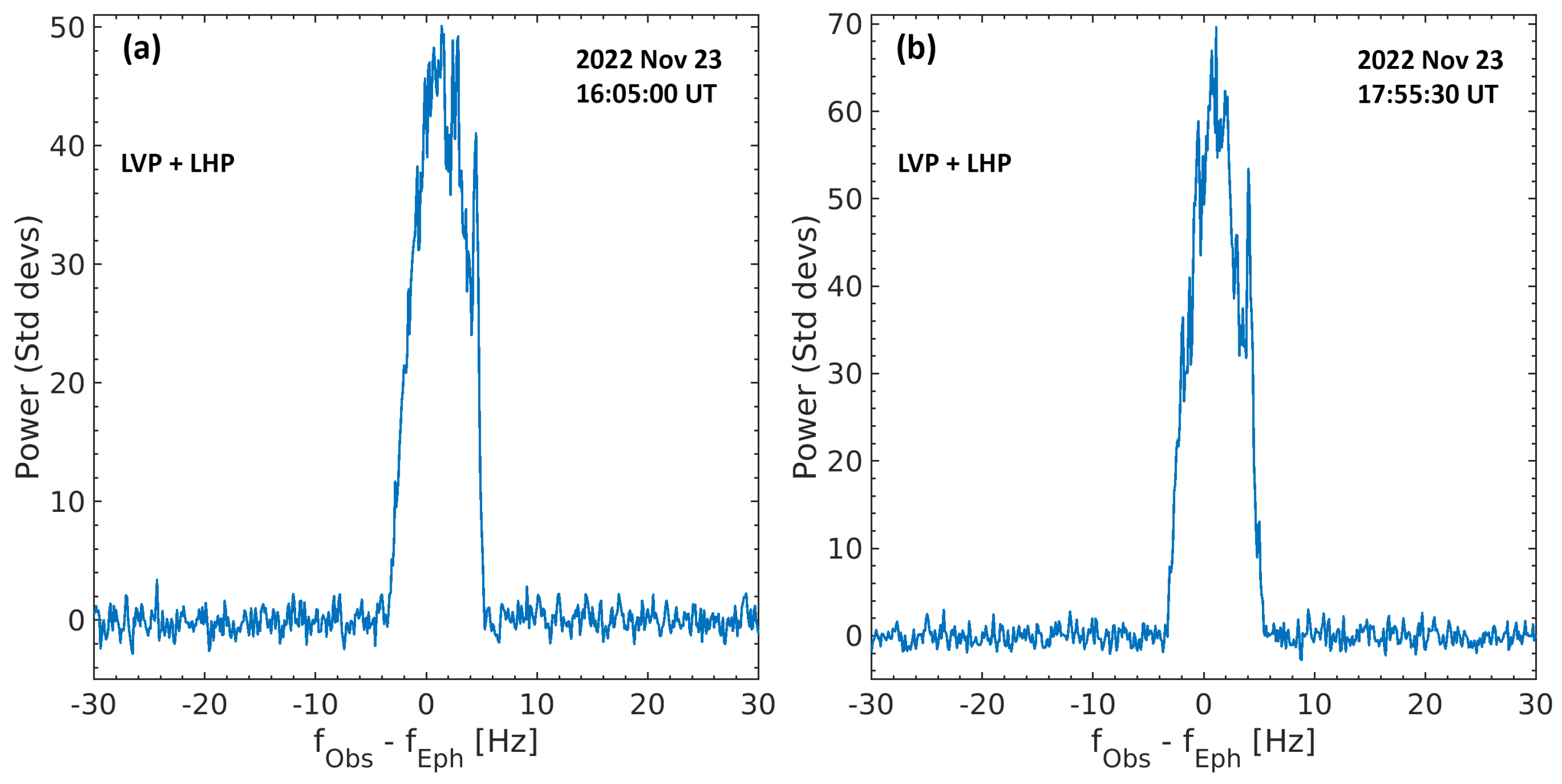
As an example, we show in Figure 12 two high-resolution (0.1 Hz) power spectra of the radar echoes acquired (a) at 16:05 UT and (b) at 17:55 UT, so approximately 1.8 h apart. This time interval corresponds to half the rotation period of the asteroid, i.e., at ${180}^{°}$ of phase angle difference. Although the two echoes refer to opposite sides of the asteroid, the spike due to the signal reflected by the secondary body is visible in both echo profiles at a frequency of ∼4 Hz. To further enhance the SNR, each spectrum is the combination of the power spectra acquired in the two linear polarization states LVP and LHP.

Figure 13 displays the full-track integrated spectrum obtained by summing incoherently all the power spectra acquired during the entire experiment. Such a long integration time almost completely covers the rotation of the asteroid, so many of the spectral features connected to the surface structure of the asteroid were averaged and smeared. Instead, the secondary peak due to the presence of the satellite was still evident. The echo spectrum was superimposed on the echo profile model [45] calculated through the multi-parametric fitting procedure.

Finally, all the echo profiles showed a displacement of the COM frequency of about $1.0\pm 0.1$ Hz with respect to the ephemeris prediction. The measurement of the frequency offset is extremely useful from an astrometric point of view, offering meaningful information to significantly improve the knowledge of the asteroids’ orbit.

6. Conclusions

We presented examples of successful radar observations of Near-Earth asteroids carried out with European radio telescopes in collaboration with NASA/JPL. They confirmed the potential of the European assets with respect to the opportunity of constituting a network for NEO observations. In particular, we here presented the results obtained on three targets, all detected with high spectral resolution:

• 2021 AF8;
• (4660) Nereus;
• 2005 LW3.

For each asteroid, we tested various processing techniques, such as the Doppler compensation performed on the time domain data via the phase-stopping method. We measured the rotation period and the echo displacement with respect to the frequency predicted by the ephemerides. For (4660) Nereus, it was also possible to measure the projected size of the asteroid at the time of observation. Finally, our observations of 2005 LW3 allowed us to detect the binary nature of the asteroids. This confirmed how the European radio telescopes can be effectively employed in NEO radar observations. Although they are heavily scheduled with other astrophysical programs, they can be involved in a selected number of radar experiments, especially when high sensitivity and high efficiency are required. These instruments are already equipped with receivers in typically employed bands, such as the C- and X-bands, but they are also provided with receivers at higher frequencies (e.g., Ka-band), which, even though they have never been used for planetary radar before, offer interesting opportunities for new solutions. Suitable backends are also available. Furthermore, the staff working at these facilities already possesses valuable know-how in radar observations and the development of post-processing software. Even though, at present, no suitable transmitting facility is available in Europe, there is significant interest in the constitution of a European network for NEO radar observations, working in synergy with USA-based facilities so as to increase the observation opportunities and provide additional contributions in the characterization of the orbits and physical properties of NEOs. A possible plan for its realization will be investigated in the near future, as monitoring the NEO population is of strategic interest for the European Union in the framework of Space Situational Awareness (SSA) activities [50] and ESA’s planetary defense activities in its Space Safety program [51].