
Spatiotemporal Characteristics of Actual Evapotranspiration Changes and Their Climatic Causes in China
 , and
, and
Abstract
:
1. Introduction
2. Materials and Methods
2.1. Materials
2.2. Methods
2.2.1. Spatio-Temporal Characteristics of ETa Changes
Theil–Sen Median Estimator and Mann–Kendall Test
Center of Gravity Migration Model
Coefficient of Variation
2.2.2. Prediction of Spatiotemporal ETa Trends
2.2.3. Attribution Analysis of ETa
Correlation Analysis
- Simple correlative analysis: this method calculates the correlative coefficient between ETa and climatic factors (precipitation and temperature [41]).
- 2.
- Partial correlative analysis: this method can effectively obviate the interference of the third factor and describe the correlation between the first two more accurately [42,43]. The correlation coefficient and partial correlation coefficient <−0.2 represent negative correlations, those >0.2 represent positive correlations, and values between the two represent weak correlations.
- 3.
Geographical Detector
Sensitivity Analysis
Contribution Analysis
3. Results
3.1. Temporal-Spatial Variations in ETa
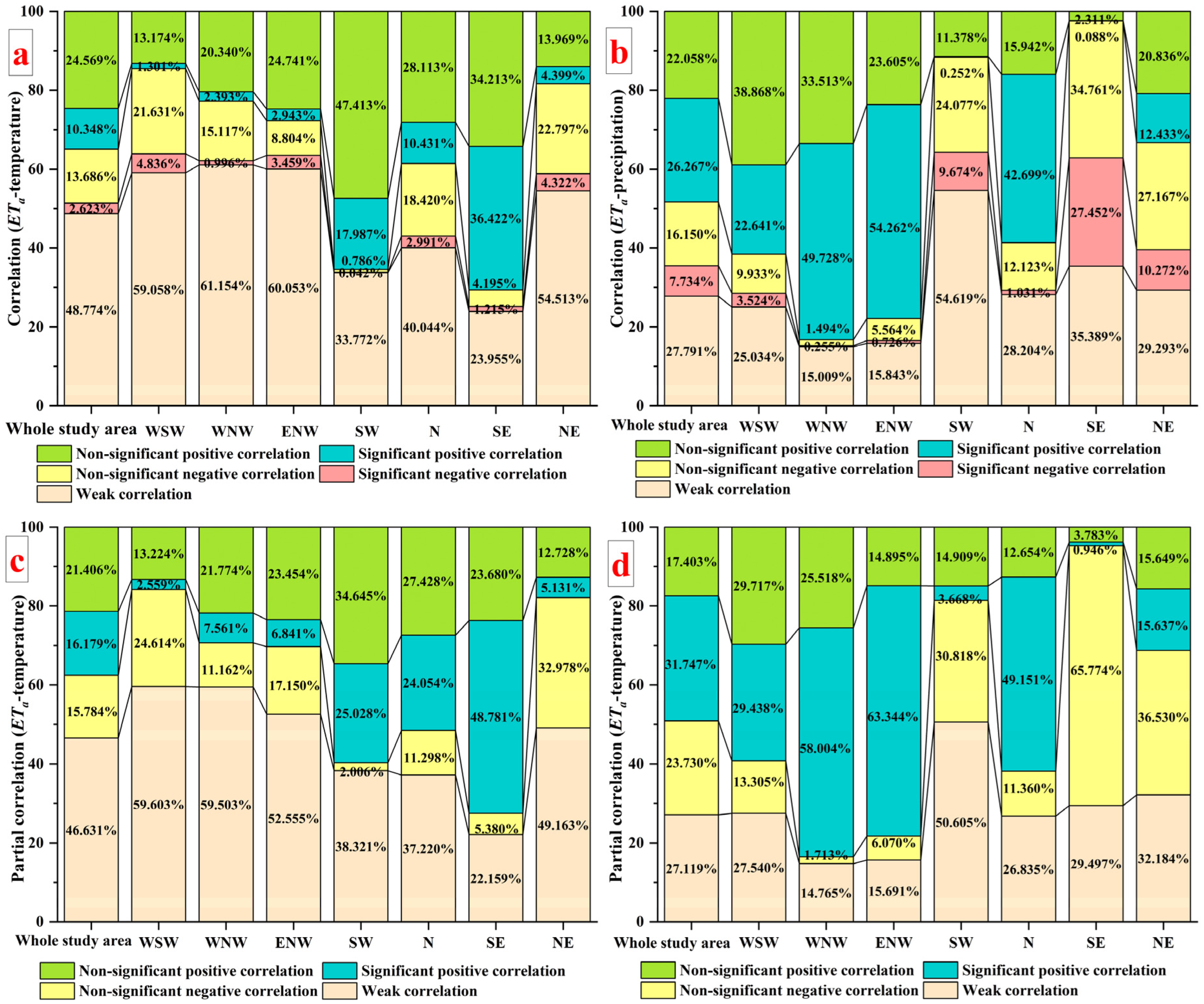
3.2. Correlation between ETa and Meteorological Factors
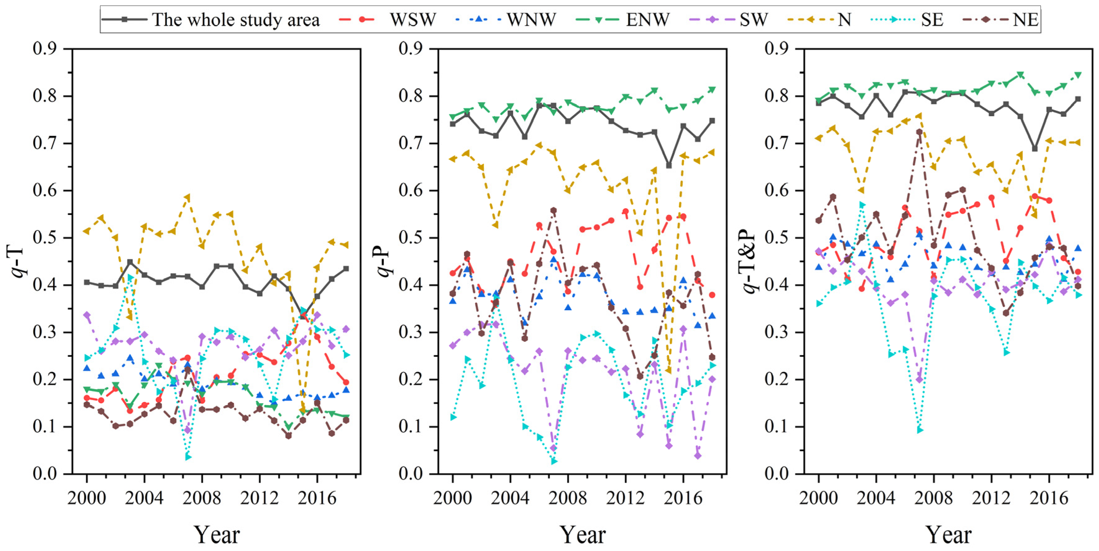
3.3. Time Variation of Factors Detected by Geographic Detectors
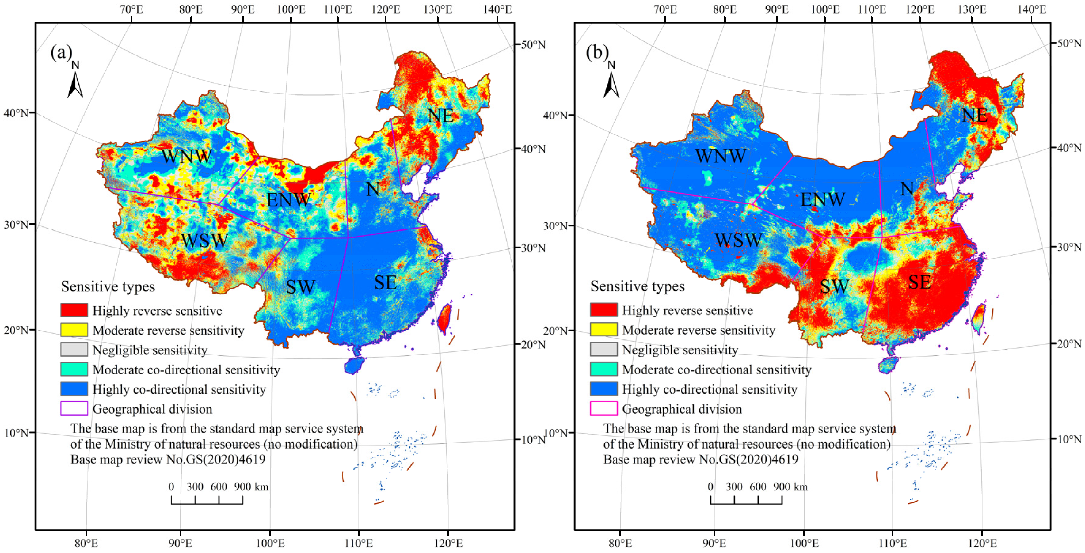
3.4. Sensitivity Analysis of ETa and Meteorological Factors
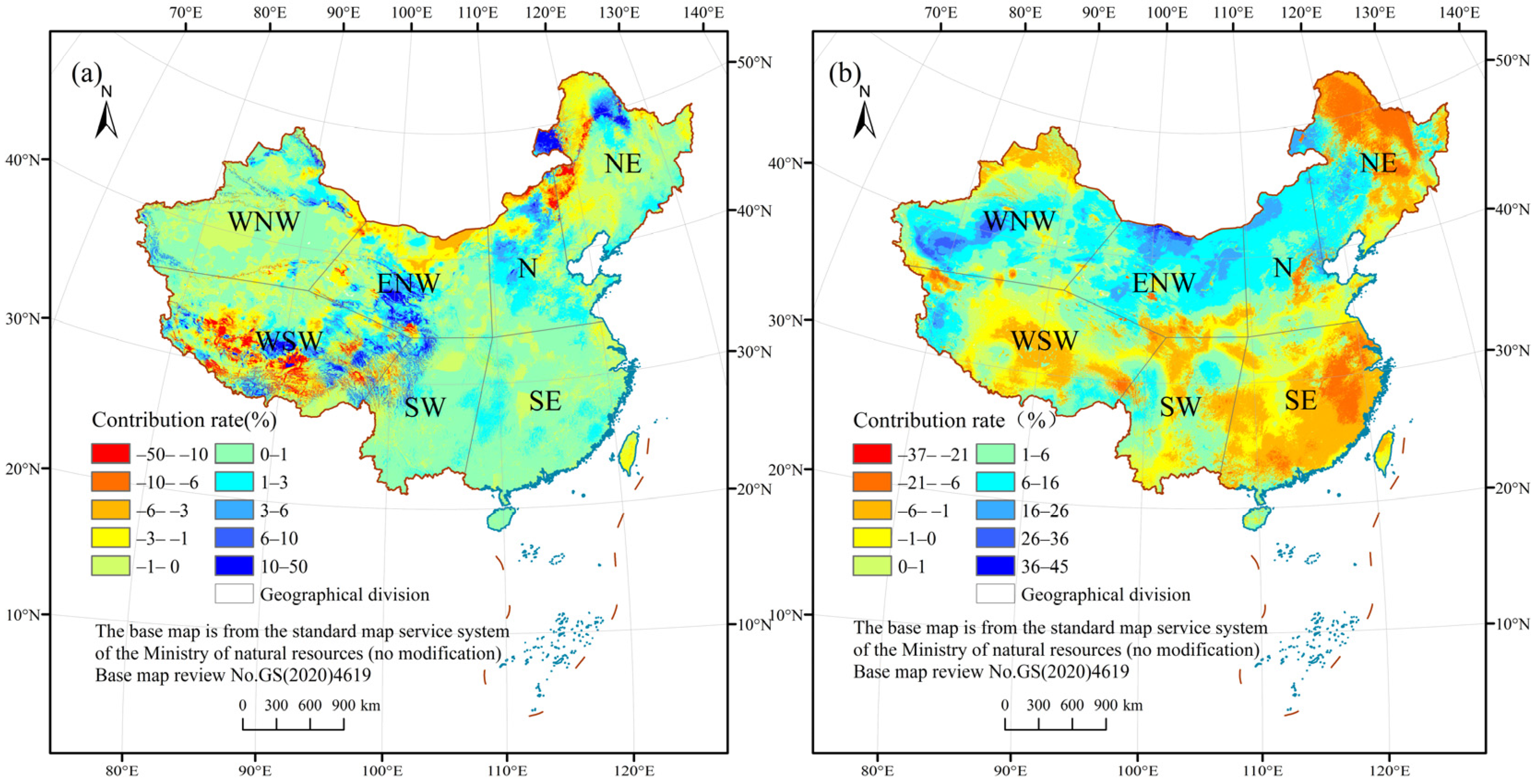
3.5. Contribution Analysis of Climate Factors to ETa
4. Discussion
4.1. The Spatiotemporal Characteristics of Evapotranspiration
4.2. Limitations and Future Prospects
5. Conclusions
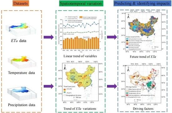
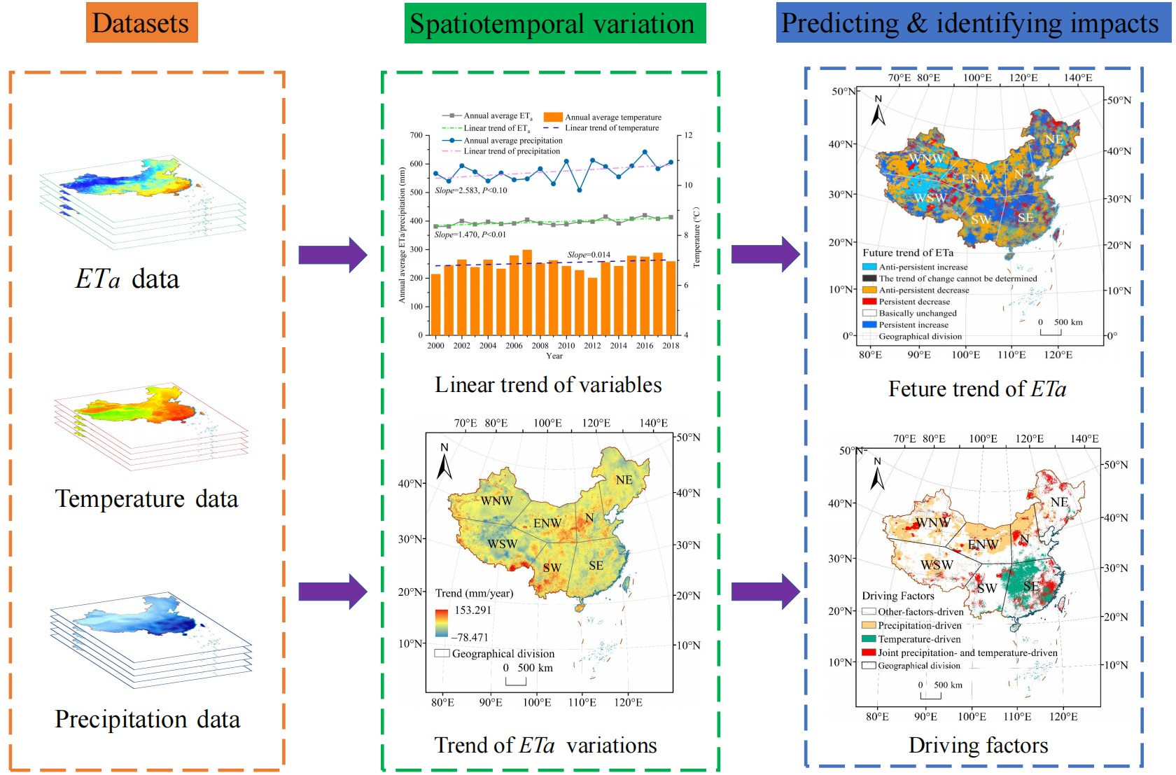
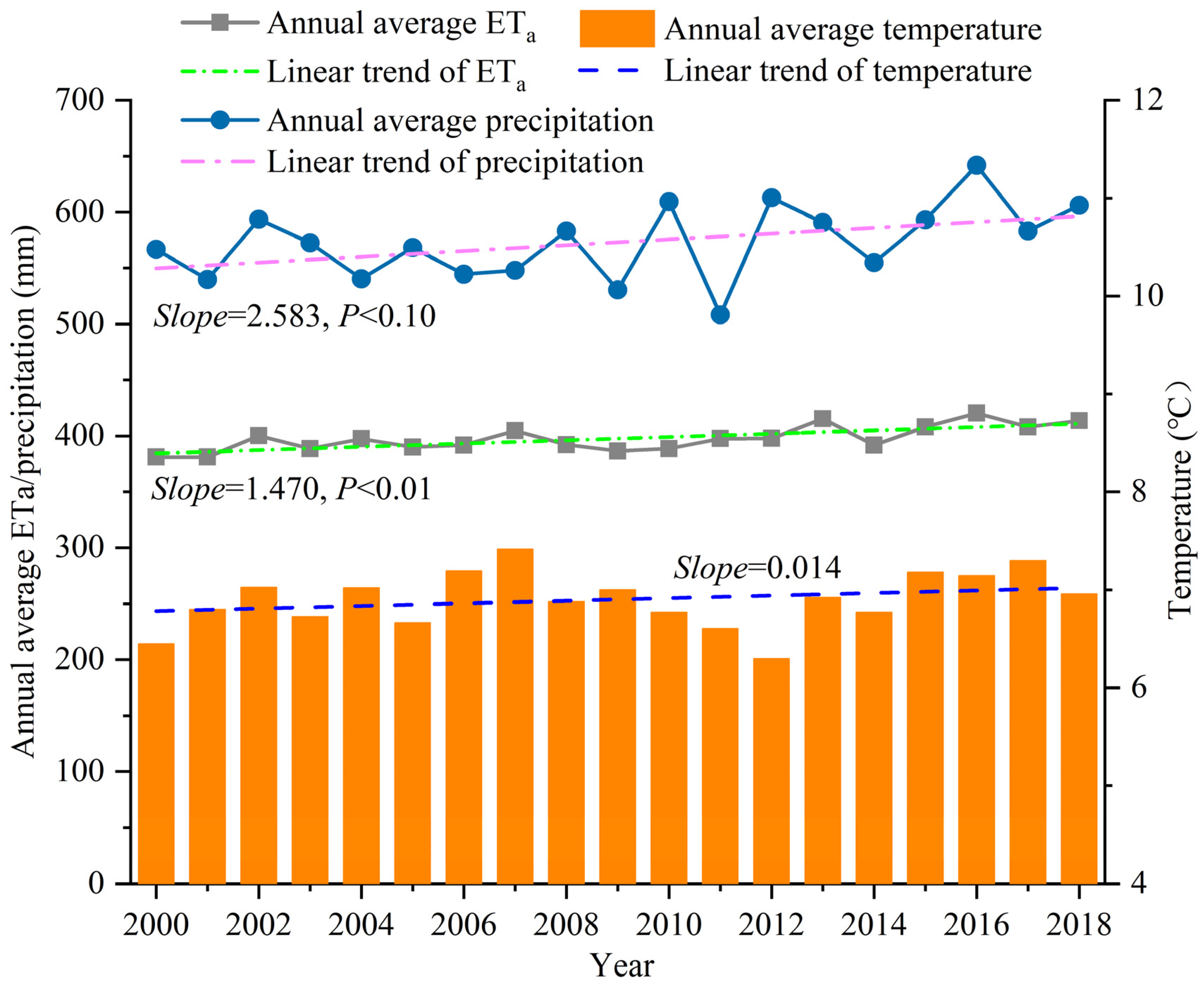
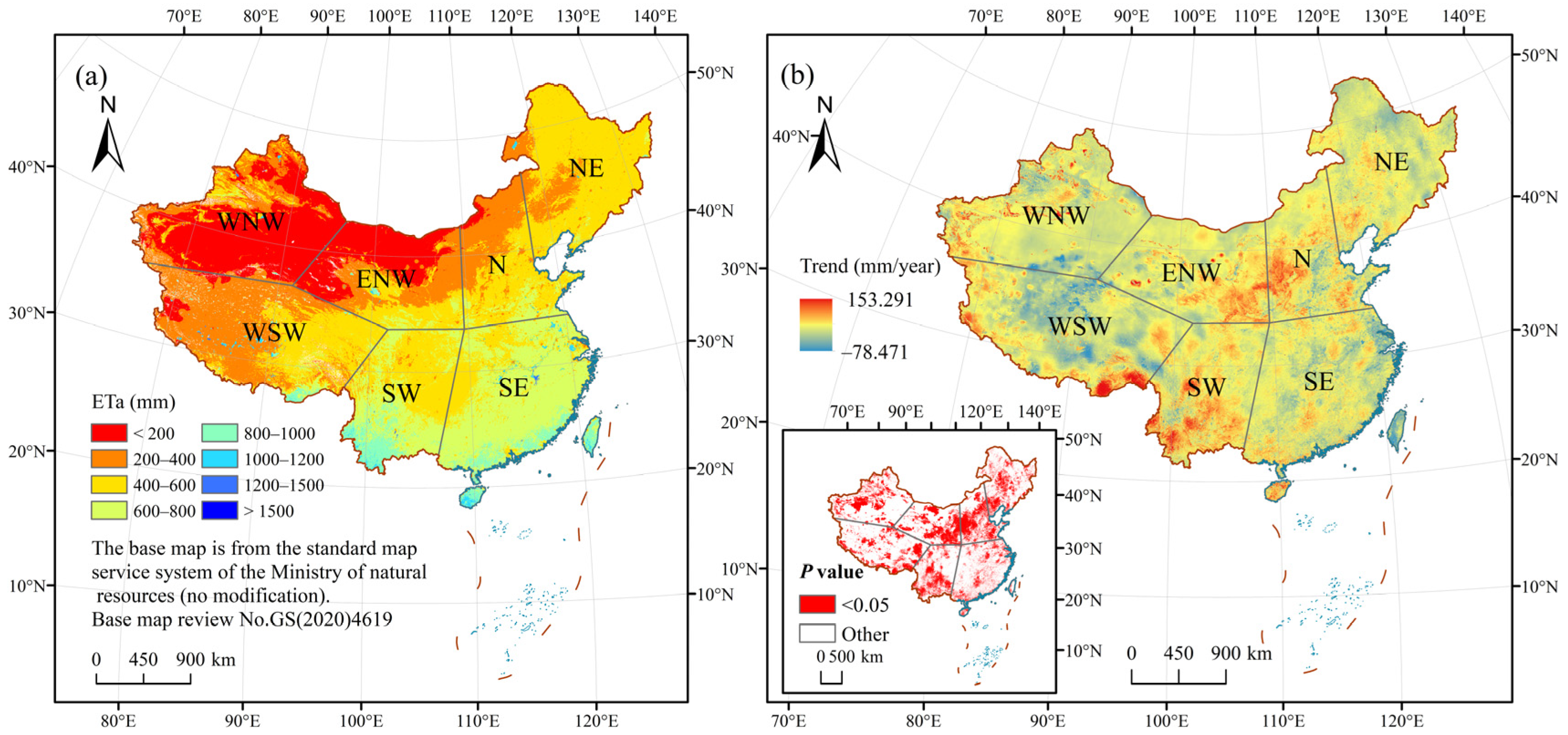
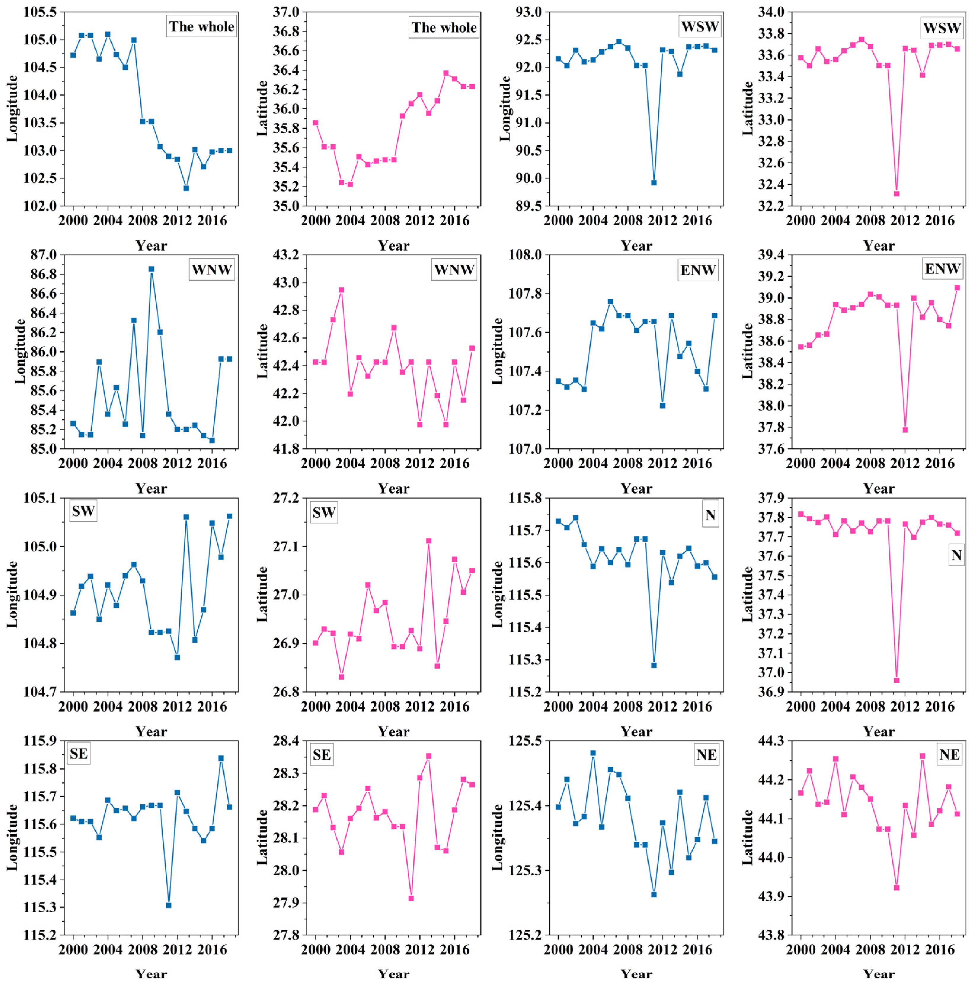
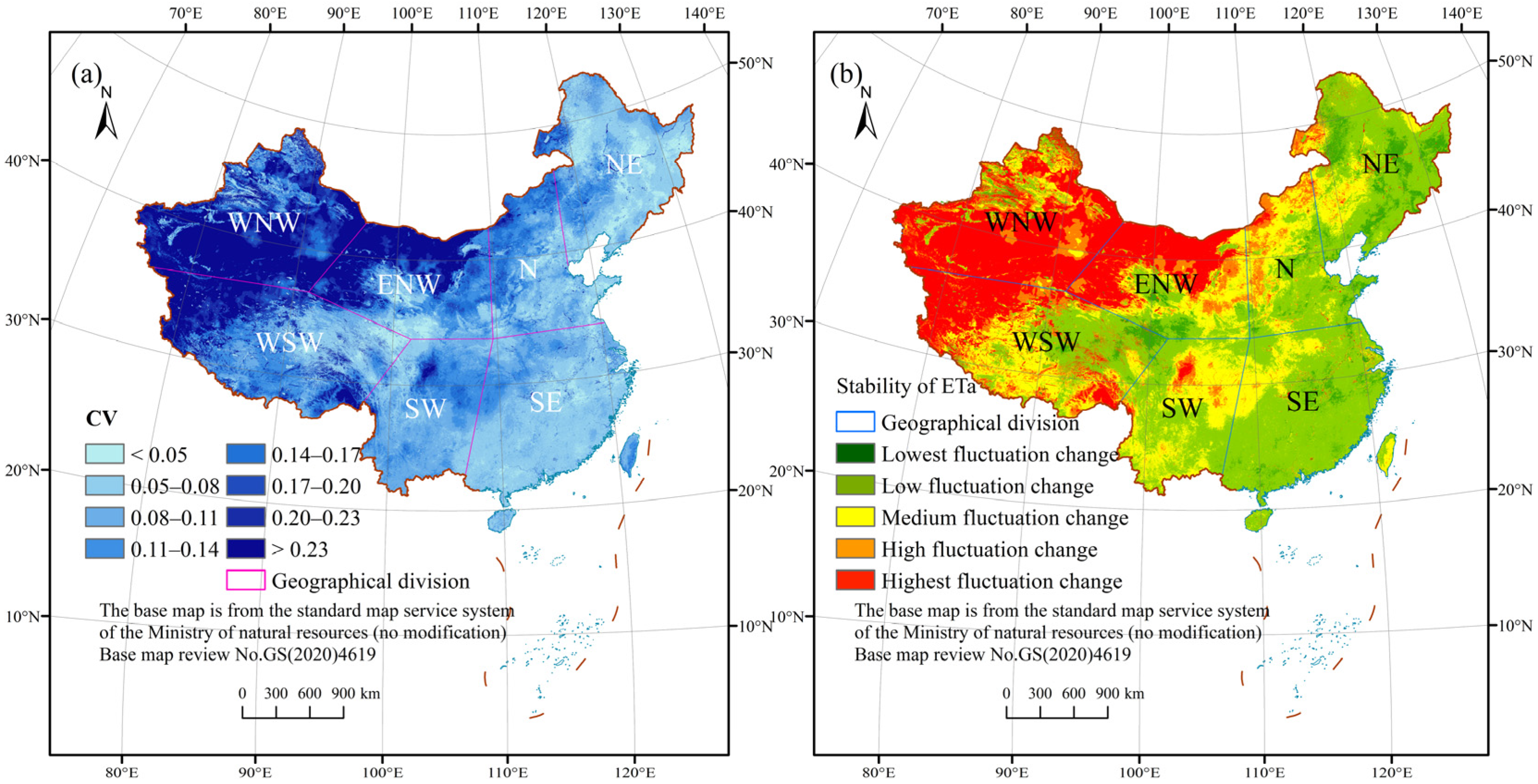
- From 2000 to 2018, the multi-year spatial mean for ETa was 397.602 mm, which showed a significant upward trend. The variation characteristics had significant spatial differences, while the southeast and northwest have high and low general distributions, respectively. The center of gravity of ETa generally shifts towards the northwest direction. The spatial distribution of the ETa variation coefficient decreased from northwest to southeast. The enforcement of public ecological restoration measures and the acceleration of urbanization may be the main reasons for ETa fluctuations.
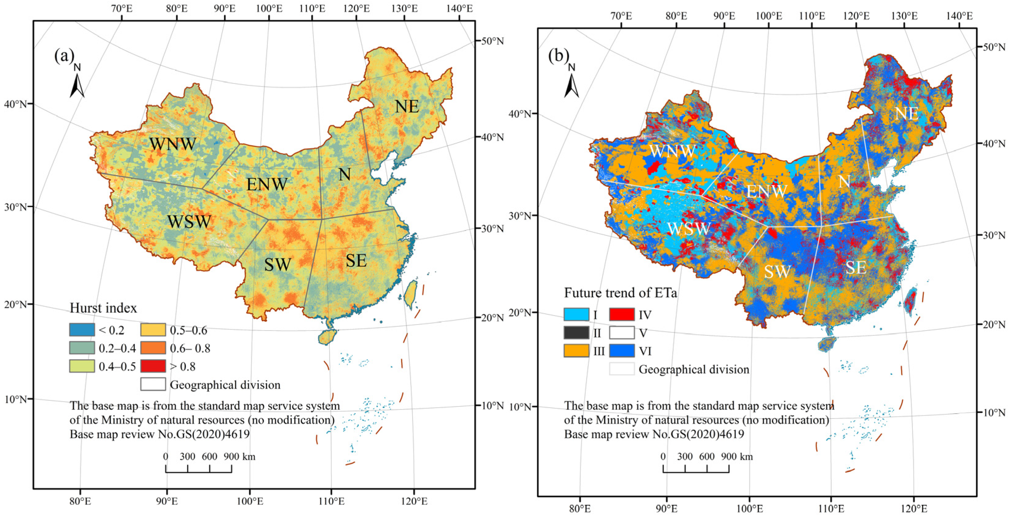
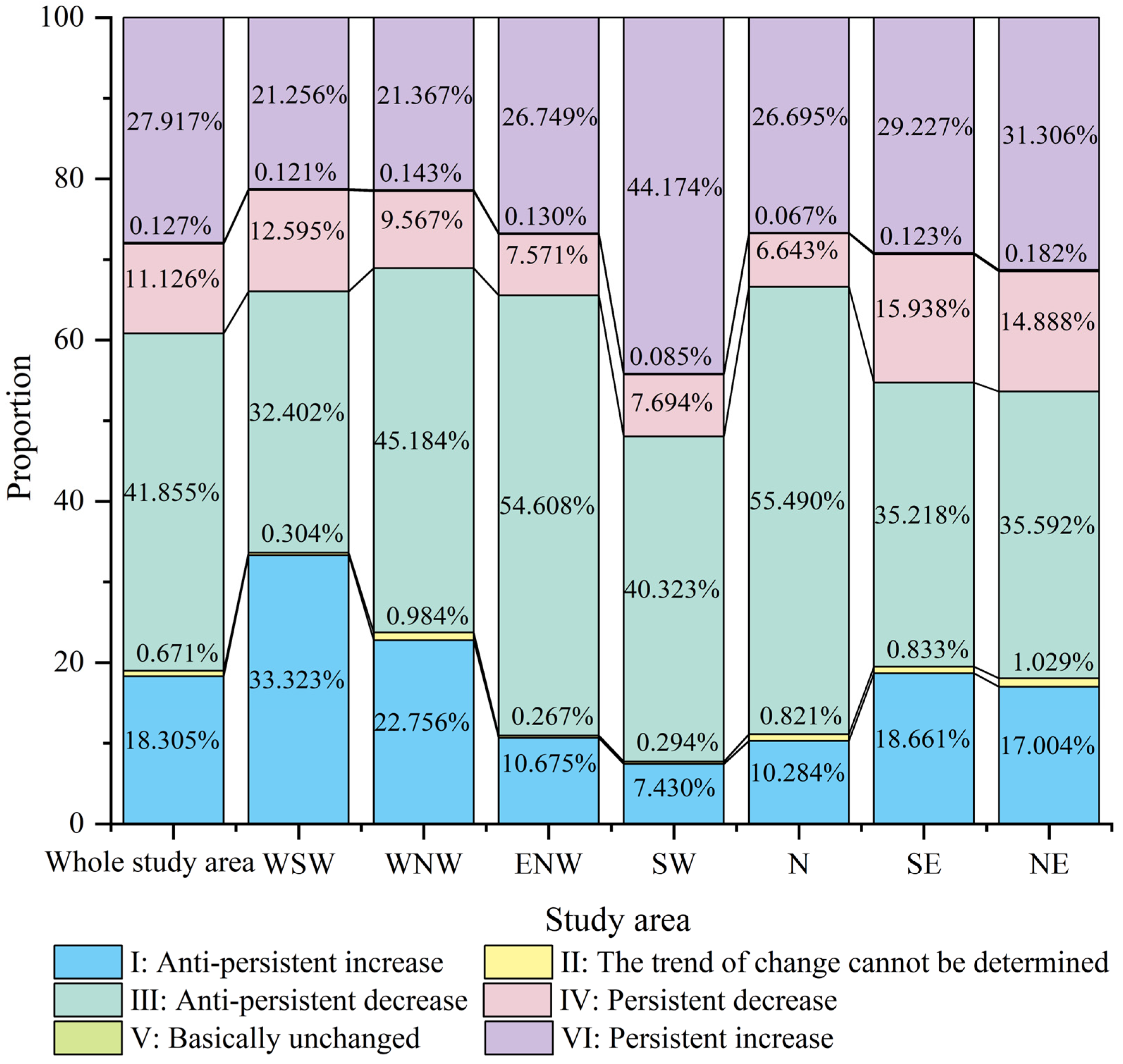
- In the future, the tendency of ETa changes in most regions will be inconsistent with the current stage. A total of 52.981% of the regional ETa will decrease to varying degrees, and the future tendency of ETa in the total area of 0.671% is still uncertain. Combined with the results of the coefficient of variation, it can be seen that the ETa in these areas fluctuated greatly from 2000 to 2018, and the complex changes make the ETa trend in this part of the region difficult to predict.
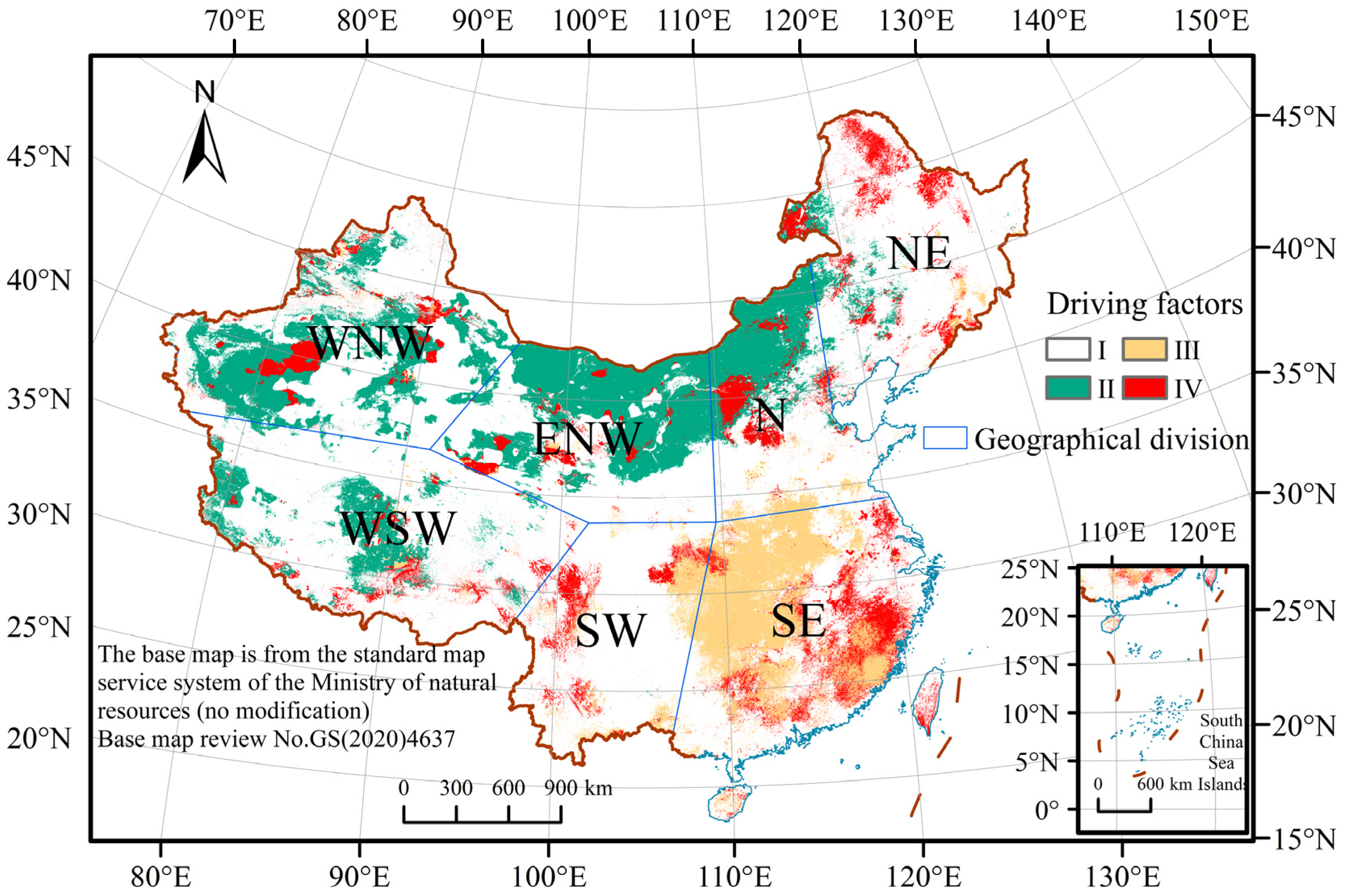
- Spatially, the correlation between ETa and precipitation was stronger than that of temperature, and precipitation had a positive correlation with ETa in more regions. In the division of ETa driving factors, the precipitation-driven region was predominantly spread in the western and northern regions, and the regional proportion was larger than the temperature-driven region. It is worth noting that in the national and seven regional studies, the driving force of the interaction between temperature and precipitation is stronger than a single factor.
- ETa was more sensitive to temperature in the southeast, while it was more sensitive to precipitation in the northwest. The coefficient for ETa sensitivity to precipitation was higher in more regions. The positive contribution area of temperature and precipitation was greater for ETa than the negative contribution area. In the southeast of China, temperature was the major cause of the ETa increase, whereas in the north and northwest, the role of precipitation was more significant.
Author Contributions
Funding
Data Availability Statement
Acknowledgments
Conflicts of Interest
References
- Luo, Y.; Gao, P.; Mu, X. Influence of Meteorological Factors on the Potential Evapotranspiration in Yanhe River Basin, China. Water 2021, 13, 1222. [Google Scholar] [CrossRef]
- Thomas, A. Spatial and temporal characteristics of potential evapotranspiration trends over China. Int. J. Climatol. 2000, 20, 381–396. [Google Scholar] [CrossRef]
- Penman, H.L. Natural evaporation from open water, bare soil and grass. Proc. R. Soc. Lond. Ser. A Math. Phys. Sci. 1948, 193, 120–145. [Google Scholar]
- Monteith, J.L. Evaporation and environment. Symp. Soc. Exp. Biol. 1965, 19, 205–234. [Google Scholar] [PubMed]
- Su, Z. The Surface Energy Balance System (SEBS) for estimation of turbulent heat fluxes. Hydrol. Earth Syst. Sci. 2002, 6, 85–100. [Google Scholar] [CrossRef]
- Ning, T.; Li, Z.; Feng, Q.; Liu, W.; Li, Z. Comparison of the effectiveness of four Budyko-based methods in attributing long-term changes in actual evapotranspiration. Sci. Rep. 2018, 8, 12665. [Google Scholar] [CrossRef]
- Priestley, C.H.B.; Taylor, R.J. On the assessment of surface heat flux and evaporation using large-scale parameters. Mon. Weather. Rev. 1972, 100, 81–92. [Google Scholar] [CrossRef]
- Zhao, W.L.; Gentine, P.; Reichstein, M.; Zhang, Y.; Zhou, S.; Wen, Y.; Lin, C.; Li, X.; Qiu, G.Y. Physics-Constrained Machine Learning of Evapotranspiration. Geophys. Res. Lett. 2019, 46, 14496–14507. [Google Scholar] [CrossRef]
- Hu, X.; Shi, L.; Lin, G.; Lin, L. Comparison of physical-based, data-driven and hybrid modeling approaches for evapotranspiration estimation. J. Hydrol. 2021, 601, 126592. [Google Scholar] [CrossRef]
- Rahimikhoob, A. Estimation of evapotranspiration based on only air temperature data using artificial neural networks for a subtropical climate in Iran. Theor. Appl. Climatol. 2010, 101, 83–91. [Google Scholar] [CrossRef]
- Reis, M.M.; da Silva, A.J.; Junior, J.Z.; Santos, L.D.T.; Azevedo, A.M.; Lopes, É.M.G. Empirical and learning machine approaches to estimating reference evapotranspiration based on temperature data. Comput. Electron. Agric. 2019, 165, 104937. [Google Scholar] [CrossRef]
- Zadeh, L.A. Fuzzy sets. Inf. Control. 1965, 8, 338–353. [Google Scholar] [CrossRef]
- Keshtegar, B.; Kisi, O.; Ghohani Arab, H.; Zounemat-Kermani, M. Subset modeling basis ANFIS for prediction of the reference evapotranspiration. Water Resour. Manag. 2018, 32, 1101–1116. [Google Scholar] [CrossRef]
- Anne, J.; Bernard, V.; Dominique, B. Neural Networks: From Black Box towards Transparent Box Application to Evapotranspiration Modeling. Int. J. Comput. Intell. Stud. 2008, 4, 163. [Google Scholar]
- Allen, R.; Pereira, L.; Raes, D.; Smith, M.; Allen, R.G.; Pereira, L.S.; Martin, S. Crop Evapotranspiration: Guidelines for Computing Crop Water Requirements; FAO Irrigation and Drainage Paper 56; FAO: Rome, Italy, 1998; Volume 56. [Google Scholar]
- Ahooghalandari, M.; Khiadani, M.; Jahromi, M.E. Developing Equations for Estimating Reference Evapotranspiration in Australia. Water Resour. Manag. 2016, 30, 3815–3828. [Google Scholar] [CrossRef]
- Xu, Y.; Xu, Y.; Wang, Y.; Wu, L.; Li, G.; Song, S. Spatial and temporal trends of reference crop evapotranspiration and its influential variables in Yangtze River Delta, eastern China. Theor. Appl. Climatol. 2017, 130, 945–958. [Google Scholar] [CrossRef]
- Guerra, E.; Ventura, F.; Snyder, R.L. Crop Coefficients: A Literature Review. J. Irrig. Drain. Eng. 2016, 142, 06015006. [Google Scholar] [CrossRef]
- Tahashildar, M.; Bora, P.K.; Ray, L.I.P.; Thakuria, D. Comparison of different reference evapotranspiration (ET0) models and determination of crop-coefficients of french bean (Phesiolus vulgaris.) in mid hill region of Meghalaya. J. Agrometeorol. 2017, 19, 233–237. [Google Scholar] [CrossRef]
- Chen, Z.; Sun, S.; Zhu, Z.; Jiang, H.; Zhang, X. Assessing the effects of plant density and plastic film mulch on maize evaporation and transpiration using dual crop coefficient approach. Agric. Water Manag. 2019, 225, 105765. [Google Scholar] [CrossRef]
- Li, S.; Wang, G.; Sun, S.; Hagan, D.F.T.; Chen, T.; Dolman, H.; Liu, Y. Long-term changes in evapotranspiration over China and attribution to climatic drivers during 1980–2010. J. Hydrol. 2021, 595, 126037. [Google Scholar] [CrossRef]
- Ma, Z.; Yan, N.; Wu, B.; Stein, A.; Zhu, W.; Zeng, H. Variation in actual evapotranspiration following changes in climate and vegetation cover during an ecological restoration period (2000–2015) in the Loess Plateau, China. Sci. Total Environ. 2019, 689, 534–545. [Google Scholar] [CrossRef] [PubMed]
- Xie, H.; Zhu, X.; Yuan, D.-Y. Pan evaporation modelling and changing attribution analysis on the Tibetan Plateau (1970–2012). Hydrol. Process. 2015, 29, 2164–2177. [Google Scholar] [CrossRef]
- Nie, T.; Yuan, R.; Liao, S.; Zhang, Z.; Gong, Z.; Zhao, X.; Chen, P.; Li, T.; Lin, Y.; Du, C.; et al. Characteristics of Potential Evapotranspiration Changes and Its Climatic Causes in Heilongjiang Province from 1960 to 2019. Agriculture 2022, 12, 2017. [Google Scholar] [CrossRef]
- Yin, L.; Tao, F.; Chen, Y.; Liu, F.; Hu, J. Improving terrestrial evapotranspiration estimation across China during 2000–2018 with machine learning methods. J. Hydrol. 2021, 600, 126538. [Google Scholar] [CrossRef]
- Tong, R.; Yang, X.; Ren, L.; Liu, Y.; Ma, M. Temporal and spatial characteristics of evapotranspiration in the Yellow River Basin during 1961–2012 and analysis of its influence factors. Water Resour. Prot. 2015, 31, 16–21. [Google Scholar] [CrossRef]
- Amantai, N.; Ding, J.; Ge, X.; Bao, Q. Variation characteristics of actual evapotranspiration and meteorological elements in the Ebinur Lake basin from 1960 to 2017. Acta Geogr. Sin. 2021, 76, 1177–1192. [Google Scholar] [CrossRef]
- Wang, A.; Lettenmaier, D.P.; Sheffield, J. Soil Moisture Drought in China, 1950–2006. J. Clim. 2011, 24, 3257–3271. [Google Scholar] [CrossRef]
- Stow, D.; Daeschner, S.; Hope, A.; Douglas, D.; Petersen, A.; Myneni, R.; Zhou, L.; Oechel, W. Variability of the Seasonally Integrated Normalized Difference Vegetation Index Across the North Slope of Alaska in the 1990s. Int. J. Remote Sens. 2003, 24, 1111–1117. [Google Scholar] [CrossRef]
- Jiang, W.; Yuan, L.; Wang, W.; Cao, R.; Zhang, Y.; Shen, W. Spatio-temporal analysis of vegetation variation in the Yellow River Basin. Ecol. Indic. 2015, 51, 117–126. [Google Scholar] [CrossRef]
- Li, C.; Li, X. Characteristics of Spatio-temporal Variation of Ecological Quality for Vegetation in China from 2000–2018. Resour. Environ. Yangtze Basin 2021, 30, 2154–2165. [Google Scholar]
- Ling, M.; Guo, X.; Shi, X.; Han, H. Temporal and spatial evolution of drought in Haihe River Basin from 1960 to 2020. Ecol. Indic. 2022, 138, 108809. [Google Scholar] [CrossRef]
- Li, Y.; Zhang, W.; Chen, Y.; Lei, T.; Li, J. Self-calibrating Palmer drought severity index-based analysis on spatial and temporal characteristics of drought from 1961 to 2015 in China. Water Resour. Hydropower Eng. 2019, 50, 43–51. [Google Scholar]
- Milich, L.; Weiss, E. GAC NDVI interannual coefficient of variation (CoV) images: Ground truth sampling of the Sahel along north-south transects. Int. J. Remote Sens. 2000, 21, 235–260. [Google Scholar] [CrossRef]
- Hurst, H.E. Long-Term Storage Capacity of Reservoirs. Trans. Am. Soc. Civ. Eng. 1951, 116, 770–799. [Google Scholar] [CrossRef]
- Jiapaer, G.; Liang, S.; Yi, Q.; Liu, J. Vegetation dynamics and responses to recent climate change in Xinjiang using leaf area index as an indicator. Ecol. Indic. 2015, 58, 64–76. [Google Scholar] [CrossRef]
- Zamani, R.; Mirabbasi, R.; Abdollahi, S.; Jhajharia, D. Streamflow trend analysis by considering autocorrelation structure, long-term persistence, and Hurst coefficient in a semi-arid region of Iran. Theor. Appl. Climatol. 2017, 129, 33–45. [Google Scholar] [CrossRef]
- Wang, H.; Mei, Z. Spatiotemporal Changes of Evapotranspiration and Their Relationship with Climate Factors in Guizhou Province. Res. Soil Water Conserv. 2020, 27, 221–229. [Google Scholar] [CrossRef]
- Dai, Q.; Cui, C.; Yao, Y.; Wang, S.; Peng, M.; Li, W.; Zhang, Q. Spatio-temporal Variation of NDVI and its Response to Climate Change in the Loess Plateau from 2000 to 2017. Taiwan Water Conserv. 2021, 69, 57–72. [Google Scholar] [CrossRef]
- Huang, G.; Wu, L.; Ma, X.; Zhang, W.; Fan, J.; Yu, X.; Zeng, W.; Zhou, H. Evaluation of CatBoost method for prediction of reference evapotranspiration in humid regions. J. Hydrol. 2019, 574, 1029–1041. [Google Scholar] [CrossRef]
- Xu, J. Mathematical Methods in Contemporary Geography; Higher Education Press: Beijing, China, 2002. [Google Scholar]
- Smith, A.A.; Welch, C.; Stadnyk, T.A. Assessing the seasonality and uncertainty in evapotranspiration partitioning using a tracer-aided model. J. Hydrol. 2018, 560, 595–613. [Google Scholar] [CrossRef]
- Wu, D.; Zhao, X.; Liang, S.; Zhou, T.; Huang, K.; Tang, B.; Zhao, W. Time-lag effects of global vegetation responses to climate change. Glob. Chang. Biol. 2015, 21, 3520–3531. [Google Scholar] [CrossRef] [PubMed]
- Wang, J.; Xu, C. Geodetector: Principle and prospective. Acta Geograph. Sin. 2017, 72, 116–134. [Google Scholar] [CrossRef]
- Hupet, F.; Vanclooster, M. Effect of the sampling frequency of meteorological variables on the estimation of the reference evapotranspiration. J. Hydrol. 2001, 243, 192–204. [Google Scholar] [CrossRef]
- Yin, Y.; Wu, S.; Chen, G.; Dai, E. Attribution analyses of potential evapotranspiration changes in China since the 1960s. Theor. Appl. Climatol. 2010, 101, 19–28. [Google Scholar] [CrossRef]
- Wu, R.; Wang, Y.; Liu, B.; Li, X. Spatial-temporal changes of NDVI in the three northeast provinces and its dual response to climate change and human activities. Front. Environ. Sci. 2022, 10, 974988. [Google Scholar] [CrossRef]
- Wang, Q.; Zhang, T.; Yi, G.; Chen, T.; Bie, X.; He, Y. Tempo-spatial variations and driving factors analysis of net primary productivity in the Hengduan mountain area from 2004 to 2014. Acta Ecol. Sin. 2017, 37, 3084–3095. [Google Scholar] [CrossRef]
- Xie, H.; Tong, X.; Li, J.; Zhang, J.; Liu, P.; Yu, P. Changes of NDVI and EVI and their responses to climatic variables in the Yellow River Basin during the growing season of 2000–2018. Acta Ecol. Sin. 2022, 42, 4536–4549. [Google Scholar] [CrossRef]
- Guo, X.; Meng, D.; Jiang, B.; Zhu, L.; Gong, J. Spatio-temporal change and influencing factors of evapotranspiration in the Huaihe River Basin based on MODIS evapotranspiration data. Hydrogeol. Eng. Geol. 2021, 48, 45–52. [Google Scholar] [CrossRef]
- Cheng, M.; Jiao, X.; Jin, X.; Li, B.; Liu, K.; Shi, L. Satellite time series data reveal interannual and seasonal spatiotemporal evapotranspiration patterns in China in response to effect factors. Agric. Water Manag. 2021, 255, 107046. [Google Scholar] [CrossRef]
- Cong, Z.T.; Yang, D.W.; Ni, G.H. Does evaporation paradox exist in China? Hydrol. Earth Syst. Sci. 2009, 13, 357–366. [Google Scholar] [CrossRef]
- Su, T.; Feng, T.; Huang, B.; Han, Z.; Qian, Z.; Feng, G.; Hou, W.; Dong, W. Long-term mean changes in actual evapotranspiration over China under climate warming and the attribution analysis within the Budyko framework. Int. J. Climatol. 2022, 42, 1136–1147. [Google Scholar] [CrossRef]
- Fu, J.; Gong, Y.; Zheng, W.; Zou, J.; Zhang, M.; Zhang, Z.; Qin, J.; Liu, J.; Quan, B. Spatial-temporal variations of terrestrial evapotranspiration across China from 2000 to 2019. Sci. Total. Environ. 2022, 825, 153951. [Google Scholar] [CrossRef] [PubMed]
- Li, X.; Zou, L.; Xia, J.; Dou, M.; Li, H.; Song, Z. Untangling the effects of climate change and land use/cover change on spatiotemporal variation of evapotranspiration over China. J. Hydrol. 2022, 612, 128189. [Google Scholar] [CrossRef]
- Zhan, Q. Characteristics of temporal and spatial changes of evapotranspiration on the Ginghai-Tibet plateau from 2001 to 2014. Sci. Technol. Inf 2017, 15, 218–219. [Google Scholar]
- He, T.; Shao, Q. Spatial-temporal Variation of Terrestrial Evapotranspiration in China from 2001 to 2010 Using MOD16 Products. J. Geo-Inf. Sci. 2014, 16, 979–988. [Google Scholar] [CrossRef]
- Wang, Z.; Xie, P.; Lai, C.; Chen, X.; Wu, X.; Zeng, Z.; Li, J. Spatiotemporal variability of reference evapotranspiration and contributing climatic factors in China during 1961–2013. J. Hydrol. 2017, 544, 97–108. [Google Scholar] [CrossRef]
- Qiu, L.; Wu, Y.; Shi, Z.; Chen, Y.; Zhao, F. Quantifying the Responses of Evapotranspiration and Its Components to Vegetation Restoration and Climate Change on the Loess Plateau of China. Remote Sens. 2021, 13, 2358. [Google Scholar] [CrossRef]
- Weng, S.; Zhang, F.; Lu, Y.; Duan, C.; Ni, T. Spatiotemporal changes and attribution analysis of evapotranspiration in the Huai River Basin. Acta Ecol. Sinca 2022, 42, 6718–6730. [Google Scholar]
- Zhao, L.; Xia, J.; Sobkowiak, L.; Li, Z. Climatic Characteristics of Reference Evapotranspiration in the Hai River Basin and Their Attribution. Water 2014, 6, 1482–1499. [Google Scholar] [CrossRef]
- Li, X.; He, Y.; Zeng, Z.; Lian, X.; Wang, X.; Du, M.; Jia, G.; Li, Y.; Ma, Y.; Tang, Y.; et al. Spatiotemporal pattern of terrestrial evapotranspiration in China during the past thirty years. Agric. For. Meteorol. 2018, 259, 131–140. [Google Scholar] [CrossRef]
- Zhang, F.; Geng, M.; Wu, Q.; Liang, Y. Study on the spatial-temporal variation in evapotranspiration in China from 1948 to 2018. Sci. Rep. 2020, 10, 17139. [Google Scholar] [CrossRef] [PubMed]
- Qiu, L.; Peng, D.; Chen, J. Diagnosis of evapotranspiration controlling factors in the Heihe River basin, northwest China. Hydrol. Res. 2018, 49, 1292–1303. [Google Scholar] [CrossRef]
- Ma, N.; Zhang, Y. Increasing Tibetan Plateau terrestrial evapotranspiration primarily driven by precipitation. Agric. For. Meteorol. 2022, 317, 108887. [Google Scholar] [CrossRef]
- Tolk, J.A.; Howell, T.A.; Evett, S.R. Evapotranspiration and Yield of Corn Grown on Three High Plains Soils. Agron. J. 1998, 90, 447–454. [Google Scholar] [CrossRef]
- Peters, E.B.; Hiller, R.V.; McFadden, J.P. Seasonal contributions of vegetation types to suburban evapotranspiration. J. Geophys. Res. Biogeosci. 2011, 116, G01003. [Google Scholar] [CrossRef]
- Miralles, D.G.; Gentine, P.; Seneviratne, S.I.; Teuling, A.J. Land–atmospheric feedbacks during droughts and heatwaves: State of the science and current challenges. Ann. N. Y. Acad. Sci. 2019, 1436, 19–35. [Google Scholar] [CrossRef] [PubMed]
- Pei, T.; Wu, X.; Li, X.; Zhang, Y.; Shi, F.; Ma, Y.; Wang, P.; Zhang, C. Seasonal divergence in the sensitivity of evapotranspiration to climate and vegetation growth in the Yellow River Basin, China. J. Geophys. Res. Biogeosci. 2017, 122, 103–118. [Google Scholar] [CrossRef]
- Liu, Y.; Jiang, Q.; Wang, Q.; Jin, Y.; Yue, Q.; Yu, J.; Zheng, Y.; Jiang, W.; Yao, X. The divergence between potential and actual evapotranspiration: An insight from climate, water, and vegetation change. Sci. Total. Environ. 2022, 807, 150648. [Google Scholar] [CrossRef]
- Ferreira, L.B.; da Cunha, F.F. New approach to estimate daily reference evapotranspiration based on hourly temperature and relative humidity using machine learning and deep learning. Agric. Water Manag. 2020, 234, 106113. [Google Scholar] [CrossRef]
- Han, D.; Wang, G.; Liu, T.; Xue, B.-L.; Kuczera, G.; Xu, X. Hydroclimatic response of evapotranspiration partitioning to prolonged droughts in semiarid grassland. J. Hydrol. 2018, 563, 766–777. [Google Scholar] [CrossRef]
- Wang, L.; Wang, G.; Xue, B.; Yinglan, A.; Fang, Q.; Shrestha, S. Spatiotemporal variations in evapotranspiration and its influencing factors in the semiarid Hailar river basin, Northern China. Environ. Res. 2022, 212, 113275. [Google Scholar] [CrossRef] [PubMed]
- Liu, Y.; Yao, X.; Wang, Q.; Yu, J.; Jiang, Q.; Jiang, W.; Li, L. Differences in Reference Evapotranspiration Variation and Climate-Driven Patterns in Different Altitudes of the Qinghai–Tibet Plateau (1961–2017). Water 2021, 13, 1749. [Google Scholar] [CrossRef]
- Ma, Y.-J.; Li, X.-Y.; Liu, L.; Yang, X.-F.; Wu, X.-C.; Wang, P.; Lin, H.; Zhang, G.-H.; Miao, C.-Y. Evapotranspiration and its dominant controls along an elevation gradient in the Qinghai Lake watershed, northeast Qinghai-Tibet Plateau. J. Hydrol. 2019, 575, 257–268. [Google Scholar] [CrossRef]
- Shen, M.; Piao, S.; Jeong, S.-J.; Zhou, L.; Zeng, Z.; Ciais, P.; Chen, D.; Huang, M.; Jin, C.-S.; Li, L.Z.X.; et al. Evaporative cooling over the Tibetan Plateau induced by vegetation growth. Proc. Natl. Acad. Sci. USA 2015, 112, 9299–9304. [Google Scholar] [CrossRef] [PubMed]
- Jin, Z.; Liang, W.; Yang, Y.; Zhang, W.; Yan, J.; Chen, X.; Li, S.; Mo, X. Separating Vegetation Greening and Climate Change Controls on Evapotranspiration trend over the Loess Plateau. Sci. Rep. 2017, 7, 8191. [Google Scholar] [CrossRef] [PubMed]
- Peng, J.; Liu, Z.; Liu, Y.; Wu, J.; Han, Y. Trend analysis of vegetation dynamics in Qinghai–Tibet Plateau using Hurst Exponent. Ecol. Indic. 2012, 14, 28–39. [Google Scholar] [CrossRef]
- Yang, Y.; Anderson, M.C.; Gao, F.; Wood, J.D.; Gu, L.; Hain, C. Studying drought-induced forest mortality using high spatiotemporal resolution evapotranspiration data from thermal satellite imaging. Remote Sens. Environ. 2021, 265, 112640. [Google Scholar] [CrossRef]
- Wang, Y.; Li, R.; Hu, J.; Wang, X.; Kabeja, C.; Min, Q.; Wang, Y. Evaluations of MODIS and microwave based satellite evapotranspiration products under varied cloud conditions over East Asia forests. Remote Sens. Environ. 2021, 264, 112606. [Google Scholar] [CrossRef]
- Karimi, S.; Kisi, O.; Kim, S.; Nazemi, A.H.; Shiri, J. Modelling daily reference evapotranspiration in humid locations of South Korea using local and cross-station data management scenarios. Int. J. Climatol. 2017, 37, 3238–3246. [Google Scholar] [CrossRef]
- Wang, L.; Kisi, O.; Hu, B.; Bilal, M.; Zounemat-Kermani, M.; Li, H. Evaporation modelling using different machine learning techniques. Int. J. Climatol. 2017, 37, 1076–1092. [Google Scholar] [CrossRef]


| Datasets | Time Range | Temporal Resolution | Spatial Resolution | Data Sources |
|---|---|---|---|---|
| Temperature (T) | 1901–2022 | monthly | 1 km | National Earth System Science Data Center |
| Precipitation (P) | ||||
| ETa | 2000–2018 | 10 days | 1 km | (https://doi.org/10.6084/m9.figshare.12278684.v5, accessed on 29 April 2022) |
| Judge Theorem | Interaction |
|---|---|
| Nonlinear weakening | |
| Single-factor nonlinear attenuation | |
| Double-factor enhancement | |
| Independence | |
| Nonlinear enhancement |
| Number | β | Hurst | Future Trend of ETa | Meaning |
|---|---|---|---|---|
| I | <−0.01 | <0.5 | Anti-persistent increase | The declining ETa in the past will increase in the future |
| II | −0.01~0.01 | <0.5 | The trend of change cannot be determined | / |
| III | >0.01 | <0.5 | Anti-persistent decrease | The increasing ETa in the past will decline in the future |
| IV | <−0.01 | >0.5 | Persistent decrease | The declining ETa in the past will persistently decrease in the future |
| V | 0.01~0.01 | >0.5 | Basically unchanged | The degree of change in ETa is relatively small |
| VI | >0.01 | >0.5 | Persistent increase | The increasing ETa in the past will persistently increase in the future |
| Driving Factors | α = 0.05 | ||
|---|---|---|---|
| Partial Correlation Coefficient (ETa-P) | Partial Correlation Coefficient (ETa-T) | Multiple Correlation Coefficient | |
| Other-factors-driven | F < F0.05 | ||
| Precipitation-driven | |t| > t0.05 | F > F0.05 | |
| Temperature-driven | |t| > t0.05 | F > F0.05 | |
| Joint precipitation- and temperature-driven | |t| < t0.05 | |t| < t0.05 | F > F0.05 |
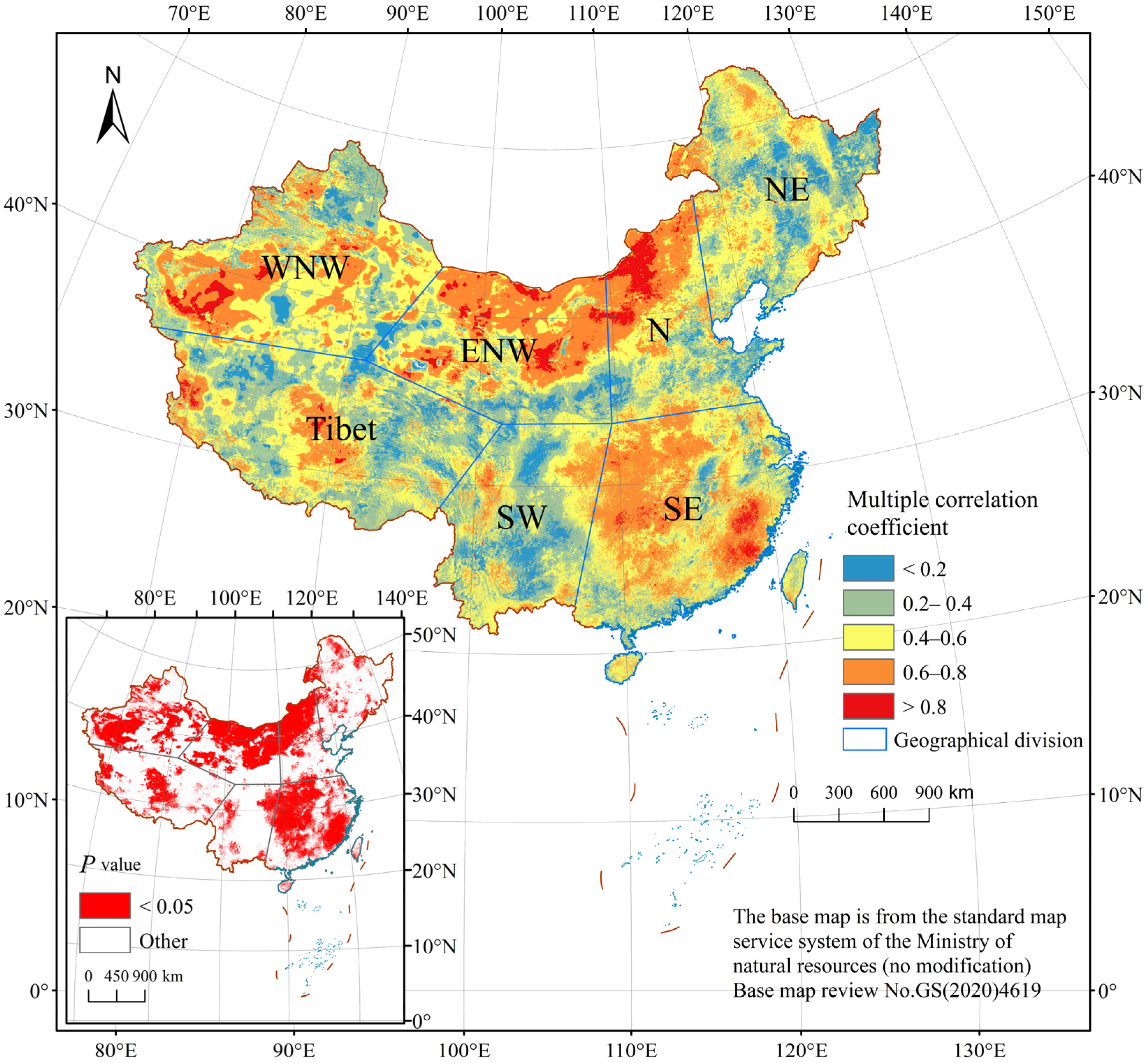
| Geographical Division | q-T | q-P | q-T&P |
|---|---|---|---|
| The whole study area | 0.407 | 0.739 | 0.779 |
| WSW | 0.214 | 0.461 | 0.499 |
| WNW | 0.191 | 0.374 | 0.458 |
| ENW | 0.166 | 0.780 | 0.818 |
| SW | 0.272 | 0.215 | 0.402 |
| N | 0.468 | 0.617 | 0.683 |
| SE | 0.258 | 0.196 | 0.370 |
| NE | 0.128 | 0.371 | 0.500 |
Disclaimer/Publisher’s Note: The statements, opinions and data contained in all publications are solely those of the individual author(s) and contributor(s) and not of MDPI and/or the editor(s). MDPI and/or the editor(s) disclaim responsibility for any injury to people or property resulting from any ideas, methods, instructions or products referred to in the content. |
© 2023 by the authors. Licensee MDPI, Basel, Switzerland. This article is an open access article distributed under the terms and conditions of the Creative Commons Attribution (CC BY) license (https://creativecommons.org/licenses/by/4.0/).
Share and Cite
Dai, Q.; Chen, H.; Cui, C.; Li, J.; Sun, J.; Ma, Y.; Peng, X.; Wang, Y.; Hu, X. Spatiotemporal Characteristics of Actual Evapotranspiration Changes and Their Climatic Causes in China. Remote Sens. 2024, 16, 8. https://doi.org/10.3390/rs16010008
Dai Q, Chen H, Cui C, Li J, Sun J, Ma Y, Peng X, Wang Y, Hu X. Spatiotemporal Characteristics of Actual Evapotranspiration Changes and Their Climatic Causes in China. Remote Sensing. 2024; 16(1):8. https://doi.org/10.3390/rs16010008
Chicago/Turabian StyleDai, Qin, Hong Chen, Chenfeng Cui, Jie Li, Jun Sun, Yuxin Ma, Xuelian Peng, Yakun Wang, and Xiaotao Hu. 2024. "Spatiotemporal Characteristics of Actual Evapotranspiration Changes and Their Climatic Causes in China" Remote Sensing 16, no. 1: 8. https://doi.org/10.3390/rs16010008