Article

Complex Validation of Weather Research and Forecasting—Chemistry Modelling of Atmospheric CO2 in the Coastal Cities of the Gulf of Finland

1
Faculty of Physics, Saint Petersburg University, St. Petersburg 199034, Russia
2
Meteoforecast Department, Russian State Hydrometeorological University, St. Petersburg 195196, Russia
3
SRC RAS—Scientific Research Centre for Ecological Safety of the Russian Academy of Sciences, St. Petersburg 197110, Russia
*
Author to whom correspondence should be addressed.
Remote Sens. 2023, 15(24), 5757; https://doi.org/10.3390/rs15245757
Submission received: 5 November 2023 / Revised: 6 December 2023 / Accepted: 14 December 2023 / Published: 16 December 2023
(This article belongs to the Section Atmospheric Remote Sensing)

Abstract

:
The increase of the CO2 content in the atmosphere caused by anthropogenic emissions from the territories of large cities (~70%) is the critical factor in determining the accuracy of emission estimations. Advanced experiment-based methods of anthropogenic CO2 emission estimation are based on the solution of an inverse problem, using accurate measurements of CO2 content and numerical models of atmospheric transport and chemistry. The accuracy of such models decreases the errors of the emission estimations. The aim of the current study is to adapt numerical weather prediction and atmospheric chemistry model WRF-Chem and validate its capability to simulate atmospheric CO2 for the territories of the two large coastal cities of the Gulf of Finland—St. Petersburg (Russia) and Helsinki (Finland). The research has demonstrated that the WRF-Chem model is able to simulate annual variation, as well as the mean seasonal and diurnal variations of the near-surface CO2 mixing ratio, in Helsinki, at a high spatial resolution (2 km). Correlation between the modelled and measured CO2 mixing ratio is relatively high, at ~0.73, with a mean difference and its standard deviation of 0.15 ± 0.04 and 1.7%, respectively. The differences between the WRF-Chem data and the measurements might be caused by errors in the modelling of atmospheric transport and in a priori CO2 emissions and biogenic fluxes. The WRF-Chem model simulates well the column-averaged CO2 mixing ratio (XCO2) in St. Petersburg (January 2019–March 2020), with a correlation of ~0.95 relative to ground-based spectroscopic measurements by the IR–Fourier spectrometer Bruker EM27/SUN. The error of the XCO2 modelling constitutes ~0.3%, and most likely is related to inaccuracies in chemical boundary conditions and a priori anthropogenic CO2 emissions. The XCO2 time series in St. Petersburg by the WRF-Chem model fits well with global CAMS reanalysis and CarbonTracker-modelled data (the differences are less than ~1%). However, due to much higher spatial resolution (2 vs. over 100 km), the WRF-Chem data are in the best agreement with the ground-based remote measurements of XCO2. According to the study, the modelling errors of XCO2 in St. Petersburg during the whole simulated period are sufficiently minimal to fit the requirement of “Error ≤ 0.2%” in 60% of cases. This requirement should be satisfied to evaluate properly the anthropogenic CO2 emissions of St. Petersburg on a city-scale.

1. Introduction

Anthropogenic CO2 emissions from the territories of large cities contribute significantly to CO2 content increases in the Earth’s atmosphere [1]. Nowadays, accurate estimation of anthropogenic CO2 emissions from the territories of large cities is an important objective. It can be useful for the evaluation of the total and regional contribution of a country to the increase of CO2 content in the atmosphere, and as a result, to the changes in CO2 radiative forcing.
Nowadays, an inventory approach is actively used to estimate emissions of greenhouse gases (GHGs) [2]. However, it was shown that on a city scale its error level can reach 100% and above [3]. In the last decade, observation-based methods have been developed and used to validate GHG inventories and provide independent estimations of the emissions of GHGs on a city-wide scale [4].
The principle of the observation-based method is based on finding a correlation between the measured increment of a gas content and its potential sources by simulating the atmospheric transport of this gas from a priori sources. The gas increment can be, for instance, measured by a differential spectroscopic approach [5,6]. In the framework of this approach, parallel measurements of the total content of the gas are carried out in upwind and downwind locations of a city using inter-calibrated spectrometers. Estimating anthropogenic emissions of CO2 using the described observation-based method is an ill-posed (in sense of Hadamard) inverse problem [5,6,7]. Examples of using this method for CO2 emission estimation (also known as inverse modelling of atmospheric transport) for specific city areas are presented in many modern studies [5,6,7,8,9,10,11,12,13].
Errors of inverse modelling significantly depend on a priori information and a direct operator. Usually, the direct operators in inverse modelling of atmospheric transport are numerical models of different complexity that model atmospheric composition. The influences of different direct operators on the solutions of inverse modelling were investigated; some of the results can be found in [14,15]. It was demonstrated that differences in numerical models of atmospheric transport cause large deviations (~50% and more) between the estimates of anthropogenic and biogenic emissions of CO2.
Box and particle dispersion models, together with spectroscopic differential observations of CO2 total columns (TC), were used in studies [5,6,12,13] to estimate the anthropogenic emissions of St. Petersburg. St. Petersburg’s megapolis is one of the largest Russian industrial cities, with a population and area of ~5 mln people and ~1400 km2, respectively [16]. There are ~10 combined heat and power plants, many industries and a large number of personal vehicles on the territory of St. Petersburg. Therefore, St. Petersburg is a large anthropogenic source of CO2. The differences between the anthropogenic CO2 emissions estimates obtained in studies [5,6,12,13] reach up to 30% and are ~1.5–2 times higher than the city’s emissions according to the inventory of anthropogenic CO2 emissions, ODIAC (Open-source Data Inventory for Anthropogenic CO2) [12,13]. Hence, it is important to set up and validate a model of atmospheric composition appropriate to the territory of interest before using it to estimate anthropogenic CO2 emissions.
WRF-Chem (Weather Research and Forecasting—Chemistry) is a numerical model for weather forecasting and the composition of the troposphere and lower stratosphere at a high spatial resolution [17]. The errors of the WRF-Chem modelling of CO2 transport have been investigated by scientists from different institutes. For instance, the mean mixing ratio of CO2 in the troposphere according to both WRF-Chem and spectroscopic measurements (IR Fourier-spectrometer Bruker 125HR, Bruker Optics GmbH & Co., Ettlingen, Germany) near Saint-Denis (France, Réunion Island, Indian Ocean) for approximately a one-year period differ by only 0.09%, with a standard deviation of 0.2% and high correlation coefficient of 0.9 [18]. Somewhat higher levels of error (0.2–0.5%) were found in a study [19] of Berlin (Germany), but only for a one-month period. In contrast to the previous study, the authors used several mobile spectrometers (Bruker EM27/SUN, Bruker Optics GmbH & Co., Ettlingen, Germany) to validate the model.
In the study described in [20], authors used in situ measurements of the near-surface CO2 mixing ratio made by a greenhouse gas analyser (GGA) [21] to validate WRF-Chem modelling of CO2 atmospheric transport in St. Petersburg. The main disadvantage of such validation is that in situ observations characterise changes of CO2 content in a relatively small air volume. Therefore, the near-surface CO2 mixing ratio is sensitive to anthropogenic emissions only during particular weather conditions. In turn, the observed CO2 total column is sensitive to all sources in the atmosphere (e.g., anthropogenic emissions, biogenic fluxes and advection), regardless of the atmospheric state. It is shown in study [22] that the mean difference between the values for column-averaged CO2 mixing ratio (XCO2) determined by the WRF-Chem model and by spectroscopic ground-based measurements for a period of more than a year in St. Petersburg is 0.6–1%, with a standard deviation of 0.5%.
Due to the possible influence of plant activity on CO2 content during the vegetation season, it is important to adapt a model to the conditions of the region of interest. For example, the territory of St. Petersburg mainly borders large areas of mixed forests and fields located in the Leningrad region and Finland [23]. According to the Annual International Geosphere–Biosphere Programme (IGBP) classification, the “mixed forest” can be characterised as a mix of four forest types—“Evergreen needleleaf forests”, “Evergreen broadleaf forests”, “Deciduous needleleaf forests” and “Deciduous broadleaf Forests”. Each of these vegetation types covers less than 60% of the landscape [24].
The aim of the current study is a complex evaluation of the WRF-Chem model designed to simulate the spatio-temporal variation of CO2 content in the atmosphere on a city-wide scale. The study is based on a comparison of the WRF-Chem-modelled data with in situ and remote ground-based observations of atmospheric CO2 content and meteorological parameters for the territories of two large cities located on the Gulf of Finland—St. Petersburg (Russia) and Helsinki (Finland). In addition, the WRF-Chem-modelled data are compared to independent modelled data provided by Copernicus Atmosphere Monitoring Service (CAMS) and NOAA’s Global Monitoring Laboratory. The data and methods are described in Section 2. The results of the WRF-Chem model validation are provided in Section 3. The conclusion of the study is given in Section 4.

2. Data and Methods

2.1. Measurements of Meteorological Parameters and CO2 Content in the Atmosphere

Remote ground-based measurements of CO2 total column (TC) were carried out in St. Petersburg in January 2019–March 2020. A measurement site is located at the Faculty of Physics of St. Petersburg State University (SPbU, 59.88°N, 29.83°E) in Peterhof. Peterhof is a part of St. Petersburg (Petrodvorcovii district) which is located ~25 km from St. Petersburg’s centre. Peterhof is set almost in the background conditions, and surrounded mainly by mixed forests and fields. In contrast to St. Petersburg’s centre, there are no large stationary sources of CO2 or intense automobile traffic on the territory of the Peterhof and Petrodvorcovii districts.
Scientists from the Finnish Meteorological Institute (FMI, Helsinki, Finland) and the University of Helsinki (UHEL) (60.20°N, 24.96°E) carry out regular observations of the CO2 mixing ratio and many other atmospheric parameters in the surface layer of the atmosphere from the roof of FMI [25]. The measurement site is located in a semi-urbanised part of Helsinki surrounded by automobile roads, parks and forests, and the built environment is mainly defined by administrative buildings. The predominant vegetation type near the station is mixed forest. Due to the relatively small distance between Helsinki and St. Petersburg (~330 km) and the quite similar mean weather conditions in these cities, the observed near-surface CO2 mixing ratio data in Helsinki are used in this study for an additional validation of the WRF-Chem model.
In addition, observations of CO2 fluxes by plants recorded at a background Finnish measurement station are used in this study. The station is positioned in Southern Finland ~180 km from Helsinki’s anthropogenic influence, and is surrounded predominantly by coniferous forest [26].
Moreover, observations of several meteorological parameters (air temperature, wind speed and direction) are used to validate the WRF-Chem model’s ability to simulate the transport of CO2 in the troposphere. Meteorological observations are carried out in St. Petersburg (Peterhof, SPbU), Voeikovo (Voeikov Main Geophysical Observatory, ~20 km from St. Petersburg’s centre and ~50 km from Peterhof) and Helsinki (FMI and UHEL). The main characteristics of the measurement systems and observation data used in this study, together with the WRF-Chem numerical experiment settings, are provided below.

2.1.1. Meteorological Parameters

Near-Surface Wind Speed and Direction

Regular observations of near-surface meteorological parameters (including wind speed and direction) have been performed at a 10 s frequency since 2018 in Peterhof (St. Petersburg) on the premises of the Faculty of Physics in SPbU. For this, a WXT536 weather station, which is located on the roof of the building (~18–20 m above ground level or agl), is used [27].
In Helsinki, observations of near-surface wind speed and direction are performed at the station SMEAR (Station for Measuring Ecosystem–Atmosphere Relations) III Kumpula [28], which is located on the roof of the Faculty of Physics of UHEL. The observations are performed at ~30 m agl [29]. A Vaisala WAA14 cup anemometer is used to observe wind parameters. The data are available with a frequency of 1 min and can be downloaded from https://smear.avaa.csc.fi (accessed on 21 January 2022).

Vertical Profiles of Wind and Air Temperature

In the Voeikov Main Geophysical Observatory (Voeikovo, Leningrad region), aerological observations of meteorological parameters (wind, air temperature, relative humidity, etc.) relative to vertical distribution are measured at 0 and 12 UTC by a radiosonde attached to a weather balloon. The observations are provided from the ground up to ~30 km and are freely available on a website [30]. The measurement site is located on the opposite side of the St. Petersburg city centre, relative to Peterhof. Therefore, the validation of the WRF-Chem model using aerological observations from Voeikovo can be helpful in analysing cases of air mass transport toward Peterhof from the most-CO2-polluted regions of St. Petersburg.
To compare the modelled and measured data, the modelled profiles of meteorological parameters were linearly interpolated to the vertical levels of the measurements (up to 50 hPa, which is WRF-Chem’s approximate upper limit). Note that it is recommended to estimate whether energy and mass are conserved after an interpolation. However, we supposed that the contribution of the vertical interpolation to the mass and energy balance deviation would be small. This is because the heights of the vertical levels of the observation data are quite similar to the heights of the levels of the original modelled data (i.e., before the interpolation). Figure 1 shows examples of air temperature and wind direction and speed in vertical profiles, derived by the observations in Voeikovo and WRF-Chem modelling, (before and after the interpolation) for 19 December 2019 12 UTC. It can be seen that the interpolated modelled profiles do not differ significantly from the original modelled profiles.

2.1.2. Near-Surface CO2 Mixing Ratio

In situ measurements of near-surface CO2 mixing ratio have been carried out on the roof of FMI, Helsinki (60.20°N, 24.95°E, ~36 m agl) since 2010 [25]. A G1301 gas analyser manufactured by Picarro, Santa Clara, California, USA [31] is used; the technique is based on cavity ring-down spectroscopy. The instrument is calibrated 2–3 times per year according to WMO/GAW standards (https://community.wmo.int/activity-areas/gaw (accessed on 30 July 2021)). The mean difference (systematic error) between this instrument and a given standard is 0.01–0.04 ppm, with a standard deviation of the mean difference (random error) of 0.02–0.07 ppm. The data are available with a 1 h frequency.

2.1.3. Column-Averaged CO2 Mixing Ratio (XCO2)

Retrieved values of the column-averaged CO2 mixing ratio (or XCO2, in ppm) are used in the study. XCO2 is calculated as the following:
X C O 2 = ( T C C O 2 ) / ( T C a i r T C w a t e r ) ,
where T C C O is a CO2 total column (TC), i.e., the number of CO2 molecules in an atmospheric column of a particular area (which usually is given in mol. cm−2); T C a i r is the number of all air molecules in the atmospheric column; T C w a t e r is the number of water molecules in the atmospheric column.
XCO2 characterises the content of CO2, on average, in the total column of dry atmosphere. By “dry” we mean that the effect of water vapour variation is mitigated by the subtraction of water vapour content from the TC of air (1). TCCO2 values are retrieved from measured spectra of incoming infrared (IR) solar radiation by a calibrated IR–Fourier spectrometer Bruker EM27/SUN [32]. This instrument measures spectra in the IR range of wavelengths (4000–12,000 cm−1) with 0.5 cm−1 spectral resolution. To interpret spectra and retrieve CO2, total columns and other parameters, the algorithm described in [32] was used. TCCO2 values are calculated as integrals of the retrieved CO2 vertical profiles. After that, Equation (1) is used to calculate XCO2. The systematic and random error levels of the retrieved XCO2 values observed by the Bruker EM27/SUN measurements and the algorithm [32] are ~0.5% and 0.025–0.075%, respectively [32,33,34].
The measurements were carried out from January 2019 to March 2020 within the framework of the international campaign EMME (Emission Monitoring Mobile Experiment) [5], with the following objectives: measurements and emission estimations of greenhouse gases for the territory of St. Petersburg [6,35]. The measurements were performed only during cloudless conditions, and therefore the dataset contains gaps during certain days and months. In total, the dataset includes 83 days of measurements for the abovementioned period. The data are available with ~1 min frequency, but for only ~3–4 h per day, with long gaps within days and months.

2.2. The WRF-Chem Model—Adaptation to St. Petersburg and Helsinki

The WRF-Chem model (Weather Research and Forecasting—Chemistry) [17] is a numerical regional model for weather prediction and the composition of the troposphere and lower stratosphere at a high spatial resolution. The modelling of CO2 transport in the atmosphere was performed for the period of January 2019–March 2020 on the territory of the Gulf of Finland and its surroundings, with a focus on St. Petersburg (Russia) and Helsinki (Finland). Complex observations of atmospheric CO2 (near-surface and total column) and meteorological parameters are available for this period of time.

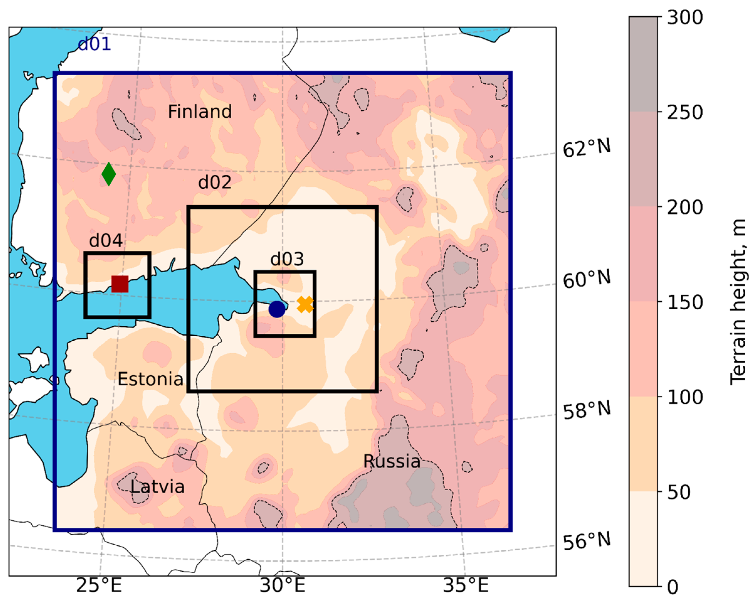
2.2.1. Description of the WRF-Chem Numerical Experiment

The modelling of CO2 transport was performed on four modelling domains, three of which are nested to the largest parent domain. This step allowed us to set boundary conditions on the inner domains with higher spatial resolution more correctly (Figure 2). The outer parent domain (d01) covers an area of 800 × 800 km2 with a space resolution (Δx) of 8 km. The area contains parts of northwest Russia, southern Finland, Estonia and Latvia. The second modelling domain (d02) is nested to d01, covering 320 × 320 km2, and Δx = 4 km. Two of the smallest domains—d03 and d04—have the same areas (110 × 110 km2) and, for both, Δx = 2 km. Moreover, d03 is nested to d02, covering St. Petersburg, while d04 is nested to d01, covering Helsinki. We nested the d04 domain only to d01 due to the following reason. Only near-surface CO2 mixing ratio is analysed in d04, which is more dependent on local CO2 emissions than on advection from the domain`s boundaries. In contrast, CO2 total content is analysed in d03, a measurement which is more sensitive to processes in the whole troposphere (e.g., advection from remote territories) than those in a surface layer. In addition, for the nesting of d04 to d02, the domains d01 and d02 have to be expanded westward to provide some space (several hundred kilometres) between the west boundaries of the d01 and d02 domains. According to our analysis, this action would significantly increase the WRF-Chem computation time. That is why the d03 domain is nested to d02 and the d04 domain is nested directly to d01.
The vertical distribution of the modelling was set to 25 hybrid levels, with the top at 50 hPa, which corresponds to ~18–20 km. This number of layers should be roughly enough to simulate the spatio-temporal distribution of CO2 in the atmosphere above St. Petersburg and Helsinki. For example, in a prior study [19], 26 vertical layers were used to simulate CO2 total columns in Berlin, Germany. A time step (Δt) constituted 40 s for d01, 20 s for d02, and 10 s for d03 and d04. To use the available observations of CO2 content in the atmosphere more effectively, the WRF-Chem-modelled data were output for every 10 min. Table 1 summarises the main parameters of the WRF-Chem numerical experiment. The current setup of the WRF-Chem model is based on several independent studies [19,36] and on our own experience [20,22].
In the current study, CO2 in the atmosphere is considered to be a fully inert gas, i.e., no CO2 chemical reactions are used in the simulation. Four main factors determining the variation of CO2 content in the atmosphere are considered. These are (1) atmospheric transport, (2) chemical boundary conditions (BCs), (3) anthropogenic emissions of CO2, and (4) CO2 biogenic fluxes due to the activity of plants (vegetation). Details of the three last factors are given in the next sections.
Initially the WRF-Chem model simulates the change of CO2 content in the atmosphere characterised by three main factors—chemical BCs, anthropogenic emissions, and biogenic fluxes. Therefore, the model output provides CO2 content as three separate variables—CO2 BCs, CO2 Ant (anthropogenic) and CO2 Bio (biogenic). The sum of the three components gives the CO2 content, which is analysed in next sections. Such an approach allows us to estimate how the total content of CO2 in the atmosphere depends on each of the three components.
XCO2 according to the WRF-Chem-modelled data is calculated by Equation (1). Above the model’s top, CO2 content was determined from the modelling data of the Copernicus Atmosphere Monitoring Service (CAMS) [37]. This step is described in Appendix A.
Table 2 shows the atmospheric processes which are parametrized on a sub-grid scale in the WRF-Chem model. Note that all processes from Table 2, except for vertical transport, were modelled by these parametrizations on each of the four modelling domains. In case of vertical transport modelling, the corresponding scheme was only used for the d01 and d02 domains (Δx 8 and 4 km, respectively). To simulate vertical transport on the two smallest domains, d03 and d04, a hydro-dynamical equation system in an approximate form was used. According to [38], such an approach is supposed to be the most correct choice when Δx < 5 km.

2.2.2. Initial and Boundary Conditions

To set initial (IC) and boundary (BC) meteorological conditions, the data of meteorological global reanalysis ERA5 [48] are used in this study. The ERA5 reanalysis data are based on numerical modelling and 4DVar assimilation of the measurements. The data have 0.25° (~25 km) spatial resolution and are spread vertically on 137 hybrid levels, covering a layer from the Earth’s surface to ~80 km [48,49]. The ERA5 data include such parameters as atmospheric pressure, wind speed and direction, air temperature, specific humidity, geopotential, etc. The meteorological BCs were set for the whole period of modelling, with a 6 h frequency.
CarbonTracker data from Near-Real Time v.2022-1 (CT-NRT.v2022-1) version [50] are used to set chemical BCs. The data consist of the CO2 mixing ratio on a global scale with a 2 × 3° (~200 × 300 km2) horizontal resolution, spreading vertically on 35 hybrid levels up to ~200 km. The CT-NRT.v2022-1 data were created by a global numerical model of atmospheric transport T5 and assimilation of observations (ground-based in situ, ship, aircraft and measurements from masts) (https://gml.noaa.gov/ccgg/carbontracker/CT2019B/ (accessed on 15 June 2021)). In the current study, the chemical BCs are set every 6 h. The CarbonTracker data were developed by scientists from NOAA ESRL, Boulder, CO, USA (http://carbontracker.noaa.gov (accessed on 15 June 2021)).

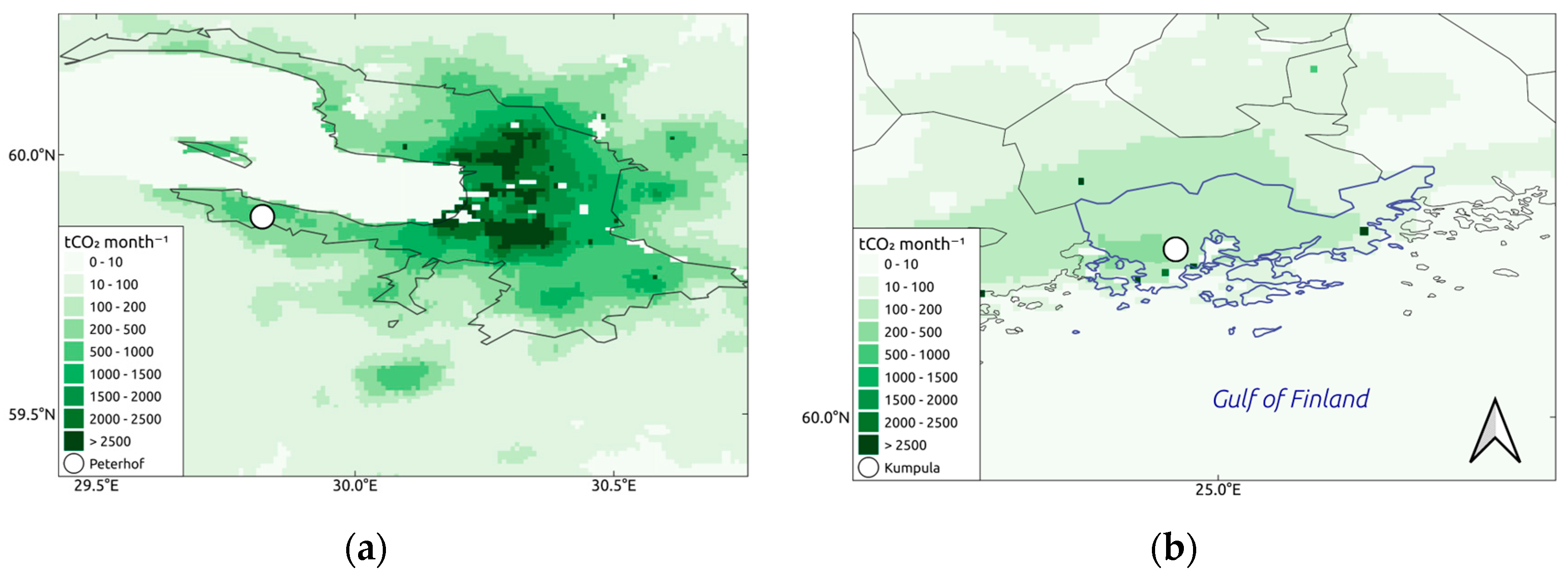
2.2.3. Sources and Sinks of CO2 Emissions

Anthropogenic Emissions
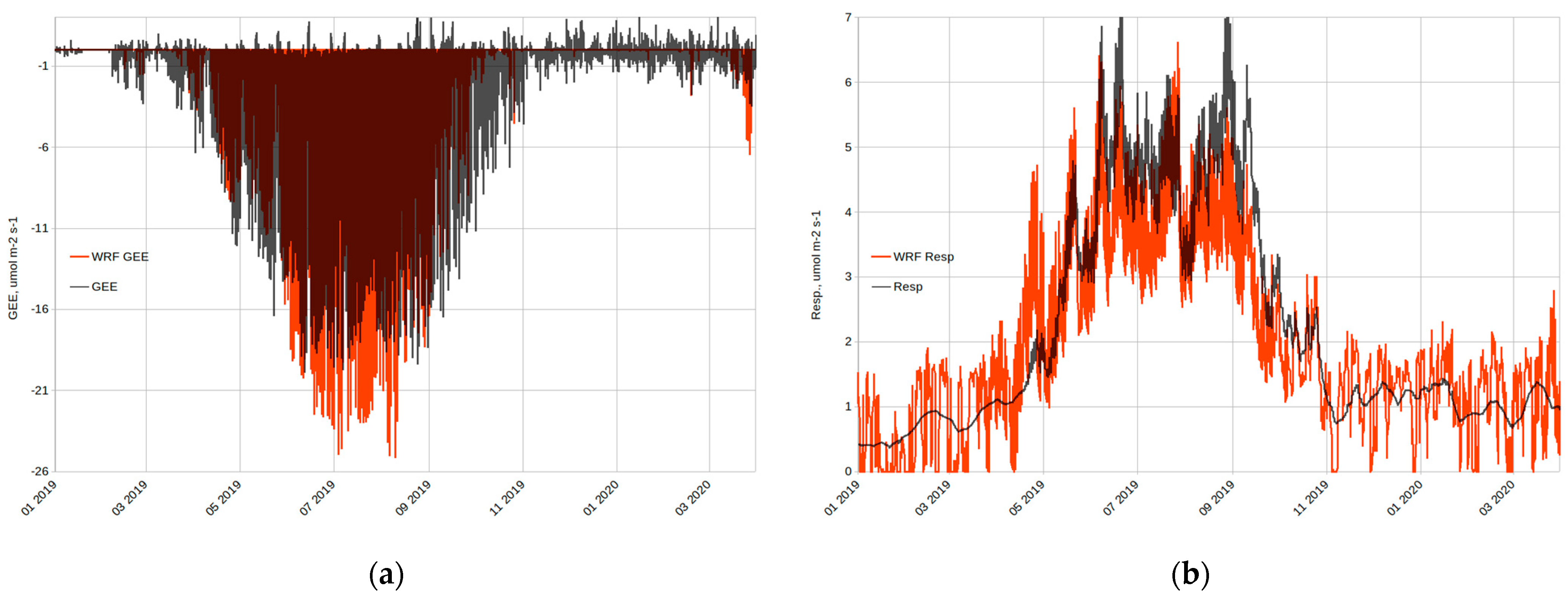
The ODIAC (Open-source Data Inventory for Anthropogenic CO2) global inventory of anthropogenic CO2 emissions, with a high spatial resolution (0.43 km2 for the modelling domain), is used in this study to set sources of anthropogenic CO2 emissions for the WRF-Chem domains [51]. The ODIAC inventory is based on official reports on the amount of fossil fuel burned by countries. Spatial discretization of the total emissions inside a particular country with a high spatial resolution is achieved by satellite observations of urban lights at night and by information on stationary sources’ locations (for example, combined heat and power plants or CHP). The ODIAC inventory for 2019 is available as total monthly anthropogenic CO2 emission per area.
Figure 3 depicts anthropogenic CO2 emissions on the territories of St. Petersburg (a) and Helsinki (b), in March 2019, in tCO2 per month according to the ODIAC inventory. The white circles in Figure 3 point to measurement stations (Peterhof and Kumpula). According to the ODIAC inventory, the spatial distribution of anthropogenic CO2 emissions in the territory of St. Petersburg is quite inhomogeneous, with a maximum in the city centre and minimum at its periphery. In contrast, anthropogenic emissions of CO2 from the territory of Helsinki are significantly lower and more spatially homogeneous. In this example, the specific anthropogenic emission of CO2 from the territory of Helsinki is ~2.3 times lower than that from St. Petersburg.
The CO2 emissions from the ODIAC inventory which, according to https://openinframap.org (accessed on 14 March 2021), corresponded to the positions of CHP in St. Petersburg and Helsinki, were placed on four lowest vertical levels of the model (heights in a range 50–200 m agl).

Biogenic Fluxes

The territories of St. Petersburg and Helsinki are surrounded by different types of vegetation—from coniferous forests to grasslands. Therefore, the biogenic factor, which is constituted by the consumption and emission of CO2 by plants, can significantly influence CO2 content in the atmosphere from the second part of spring to the beginning of autumn [52]. The Vegetation Photosynthesis and Respiration Model (VPRM) is used in the WRF-Chem simulation to consider the consumption and release of carbon dioxide by plants [53]. The VPRM is a part of the WRF-Chem model. Both models run simultaneously.
The VPRM allows us to estimate the CO2 consumption by plants due to photosynthesis (Gross Ecosystem Exchange or GEE) during daytime and CO2 release in the night-time (Respiration or Resp) for seven types of vegetation. The sum of GEE and Resp (Net Ecosystem Exchange or NEE) determines whether plants act as a source of CO2 or a sink. A more detailed description of the model can be found in [53]. In the framework of the VPRM, the parameters GEE and Resp are functions of near-surface air temperature, reflected shortwave solar radiation in particular ranges of wavelengths, and the amount of photosynthetically active radiation consumed by plants. The reflected shortwave solar radiation data are measured by the Moderate Resolution Imaging Spectroradiometer (MODIS), which is onboard the Aqua and Terra satellites (product MCD12Q1 v006, https://lpdaac.usgs.gov/products/mcd12q1v006/ (accessed on 12 December 2022)). The satellite data are available with an 8 day-frequency.
In the current study, the VPRM was partially optimised by the correction of the Resp parameter using the corresponding measurements from the background Finnish observation station “SMEAR II Hyytiälä Forest”. The correction was provided only for one of seven vegetation types—needleleaf forest. The trees of this type are predominant in the area of the station. The characteristics of the CO2 biogenic fluxes according to the measurements at the SMEAR station are described in Appendix B.
The parameter Resp in the VPRM is calculated by linear regression from near-surface air temperature (Tair). The parameters of linear regression (a and b) are fitted for a particular vegetation type based on the measurements of Tair and Resp. Table A1 in Appendix B contains the original values of the regression parameters, and those corrected to the conditions of Hyytiälä.
Figure A1 in Appendix C demonstrates the time series of GEE and Resp by the VPRM modelling in the framework of the WRF-Chem run, as well as the measurements at the Hyytiälä station, for March 2019–January 2020. The correlation coefficient is ~0.9. On average, the model underestimates and overestimates GEE and Resp by 11.7 and 6.9%, respectively. The maximum differences were found in summer, i.e., during the peak of the vegetation season.

Other Sources and Sinks of CO2

Another possible factor influencing CO2 content is absorption and emission of the gas by a water surface. St. Petersburg and Helsinki are located on the shore of a large water body—the Gulf of Finland. To estimate the possible influence of the water surface of the Gulf of Finland on CO2 content in St. Petersburg, a prior study [54] was carried out. In this study, the CO2 fluxes from the Gulf of Finland were investigated using methods from independent studies and ship-based observation data.
The study has demonstrated that the possible contribution of the gulf’s water surface to the atmospheric CO2 content is very small in relation to anthropogenic emissions (1.7–3%). Therefore, in the current study the contribution of the water body to the atmospheric CO2 content was neglected.
The contribution of biomass burning to the CO2 content is set implicitly via chemical BCs on the largest modelling domain (d01).

2.2.4. Correction of the Chemical Boundary Conditions

According to analysis, the CarbonTracker data (ICs and BCs in the WRF-Chem model run) overestimate XCO2 by ground-based remote measurements in Peterhof during January 2019–March 2020 by 3.3 ppm, with a standard deviation of 1.3 ppm (Figure 4). This can be related to errors in a priori anthropogenic emissions of CO2, crude spatial resolution of the modelling, etc. Therefore, the CarbonTracker data should be corrected before using them as chemical ICs and BCs in the WRF-Chem simulation for the territory of the current study.
However, it is impossible to directly compare the CarbonTracker data with the measured CO2 total column (TC) on the boundaries of the parent modelling domain since there are no corresponding observations in these regions. Let’s assume that CO2 content in an air mass which is advected to St. Petersburg is influenced only by advection from a remote territory (for example, from the domain’s boundaries). Such conditions can be achieved if there are few large anthropogenic sources of CO2 and weak fluxes by vegetation on the path of the air mass moving toward St. Petersburg. Therefore, to use the available CO2 observations in St. Petersburg, the pairings of XCO2 in the city from CarbonTracker and the measurements were filtered according to those two conditions.
In a previous study [55], it was shown that with particular directions of the near-surface wind, ground-based remote observations of CO2 TC in Peterhof registered the anthropogenic contribution of the centre of St. Petersburg to the CO2 content in the atmosphere. Hence, to filter the data by the first condition, ground-based measurements of XCO2 and near-surface wind direction in Peterhof were analysed. The measurements of TC CO2 when the near-surface wind direction corresponded to atmospheric transport from the territory of St. Petersburg (20–150°) were excluded from the further correction of the CarbonTracker data. To consider the second filtering condition, the data were filtered by the period when the biogenic influence on CO2 content would be at its maximum. According to the VPRM, this is the period from the beginning of spring to the middle of autumn.
The filtration reduced the dataset from 128 to 14 pairs of XCO2 values by the CarbonTracker and measurement data in St. Petersburg for January 2019–March 2020. At this point, it can be said that the filtered values of XCO2 characterise the TC CO2 in St. Petersburg, which, in general, was influenced by air mass transport from the boundaries of the WRF-Chem modelling domain. The mean difference (MD) between the filtered pairs constitutes −1.8 ppm (~−0.4%), which means that the CarbonTracker data overestimate observed XCO2 values. Therefore, chemical BCs (the CarbonTracker data) were reduced by 0.4%.

2.3. Independent XCO2 Modelling Data in St. Petersburg

The global reanalysis of atmospheric CO2 by the Copernicus Atmosphere Monitoring Service (CAMS), version v21r2 [37], was used in the study as independent modelled data. The data have horizontal resolution of 1.86 × 3.75° (~200 × 400 km2), spreading vertically on 39 hybrid levels up to ~70 km agl. The data are available for the whole period of investigation with a 3 h frequency. The CAMS reanalysis was made using a numerical model of global atmospheric transport with assimilated ground-based measurements of near-surface CO2 content [56].

3. Results and Discussion

3.1. Comparison between Modelling and Measurement Data

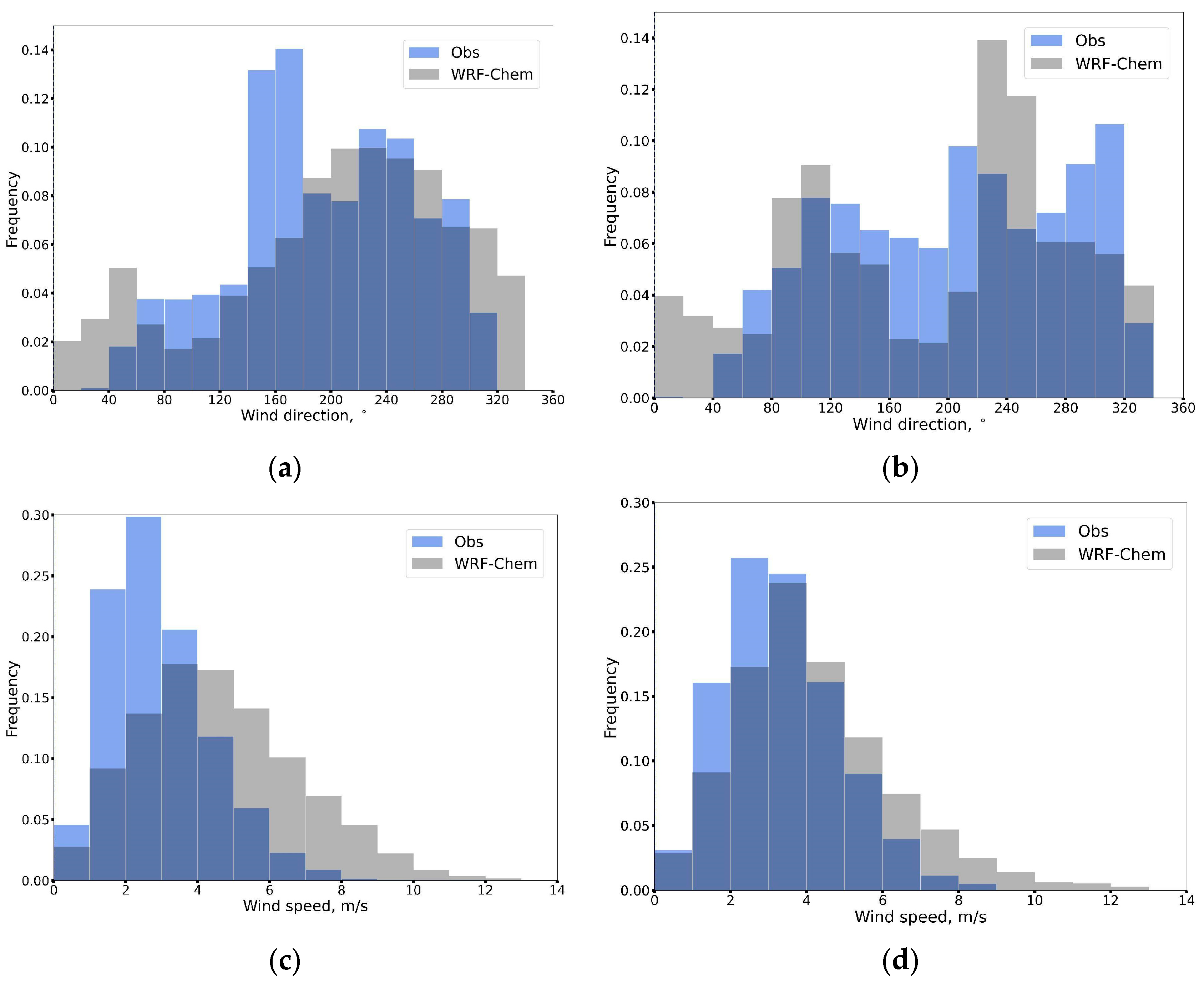
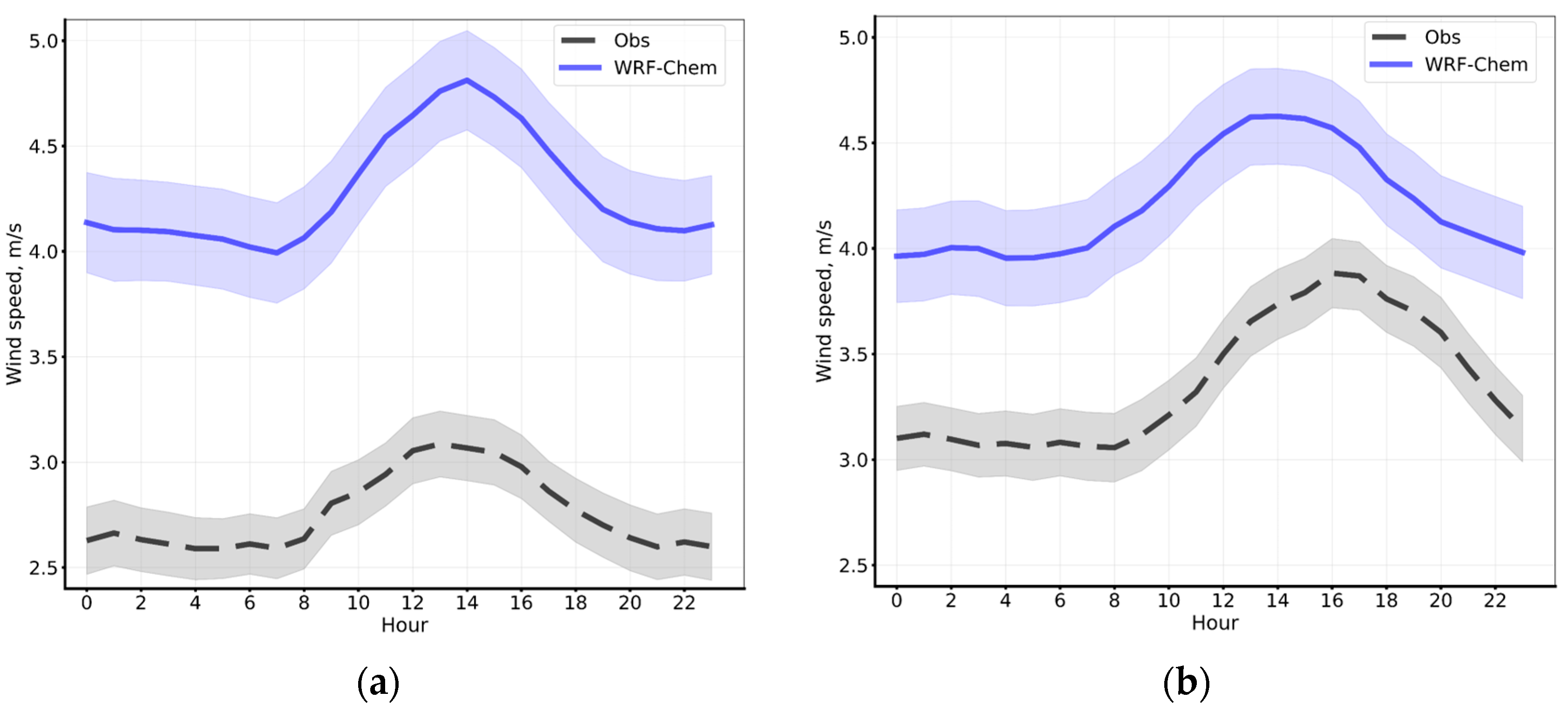
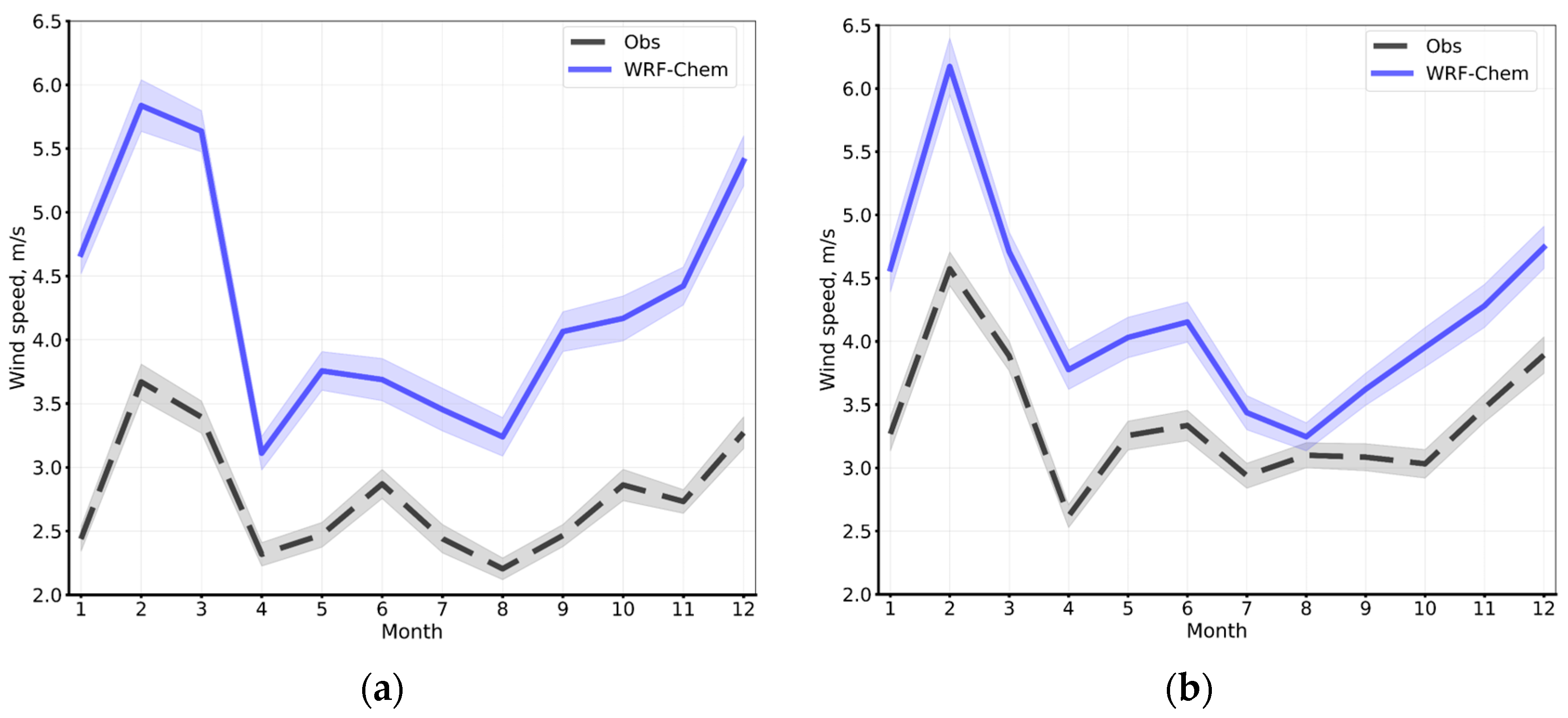
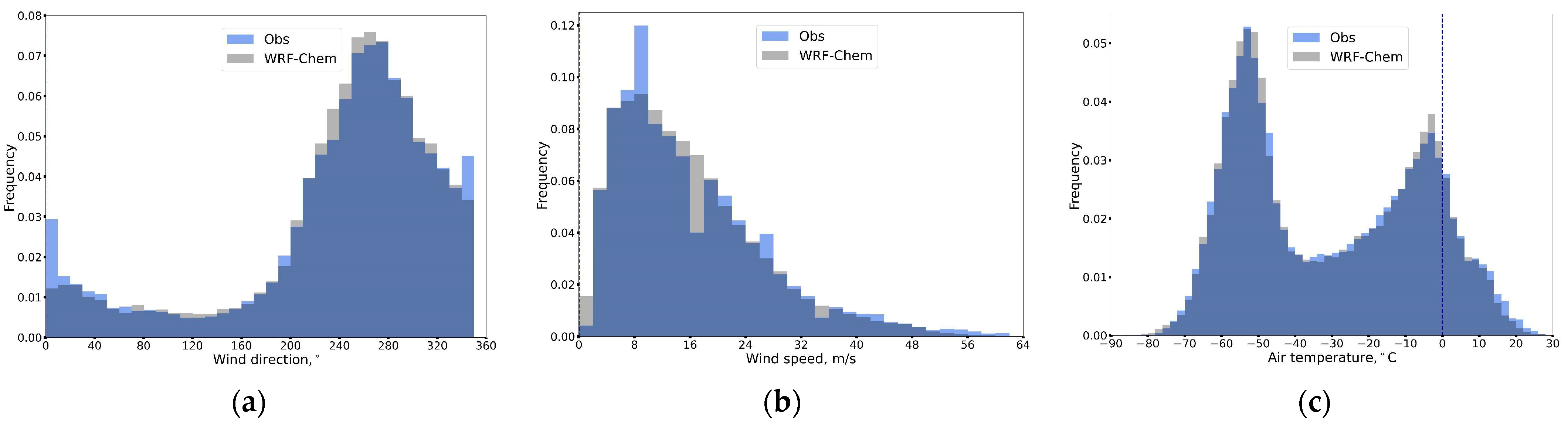
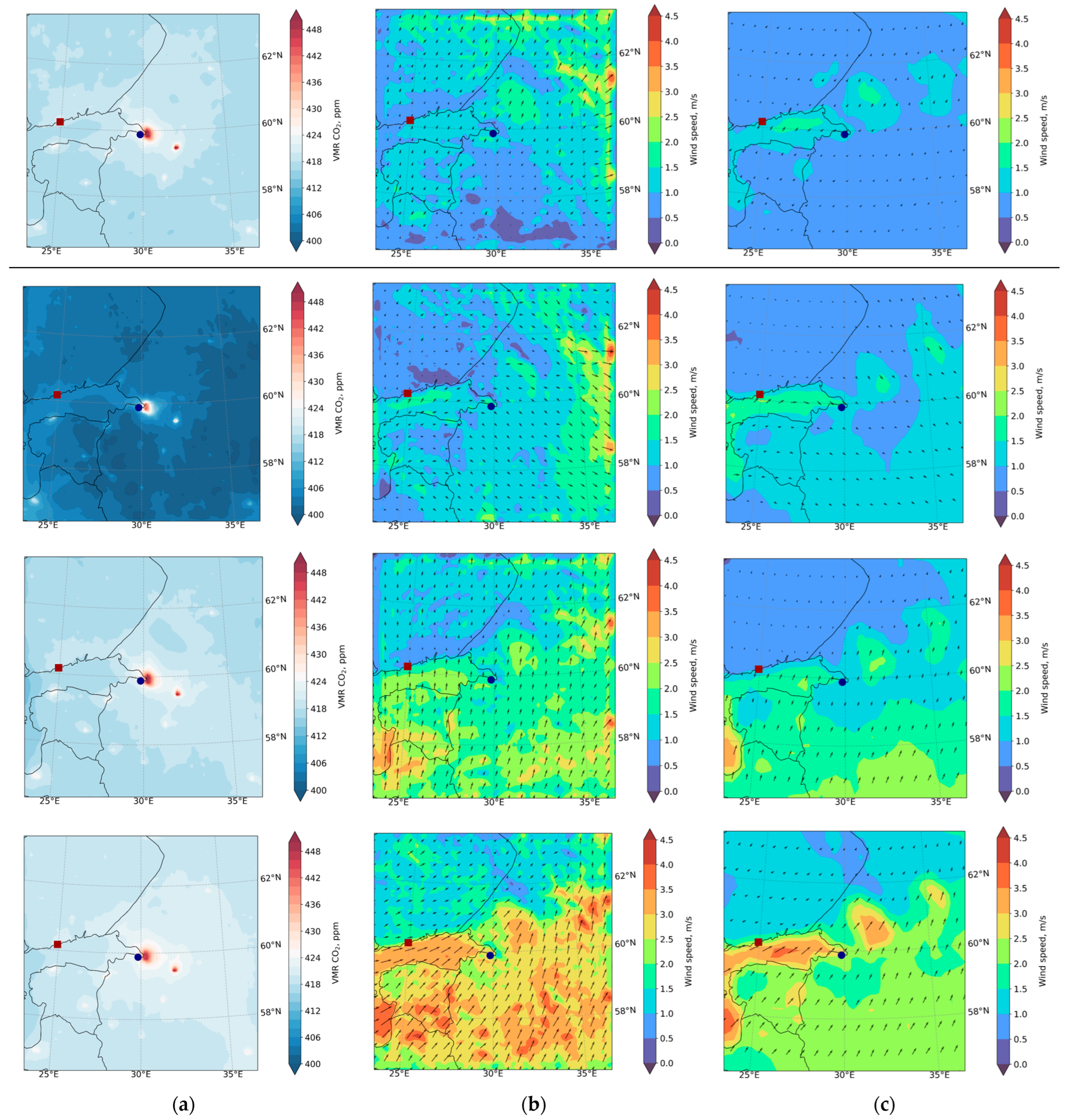
3.1.1. Near-Surface Wind Speed and Direction

The WRF-Chem model simulates near-surface (10 m) wind speed and direction in St. Petersburg and Helsinki with rather different errors. The mean differences (MDs) are −1.7 m/s and 38.2° for St. Petersburg and −0.8 m/s and 21.6° for Helsinki. The standard deviation of the difference (SDD) of wind speed is almost the same in both cities, at 1.5–1.6 m/s. However, the SDD of wind direction is higher in Helsinki (48.2°) than in St. Petersburg (29.3°). Probable reasons for the WRF-Chem model to overestimate near-surface wind speed include higher uncertainties in the simulations of windless conditions (e.g., during winter) [57,58]. In addition, the overestimation of near-surface wind speed by the WRF-Chem model relative to observations can be caused by local small-scale tropospheric circulations due to the proximity of St. Petersburg and Helsinki to the Gulf of Finland [59] and Ladoga Lake (on the west). Correlation coefficients (CC) between the modelled and measured near-surface wind speed and direction are, respectively, 0.76 and 0.8 in St. Petersburg and 0.67 and 0.78 in Helsinki. Similar estimates are provided in [18,60].
Figure 5 demonstrates histograms of the distribution of near-surface wind direction and speed in St. Petersburg (January 2019–March 2020) and Helsinki (2019) according to the WRF-Chem modelling and observations. First, note how different the wind direction distribution is in the two cities. Wind directions 140–180° (SSE-S) and 220–260° (WSW) (Figure 5a) with a wind speed of 1–4 m/s (Figure 5c) are predominant in St. Petersburg. The distribution of near-surface wind direction in Helsinki (Figure 5b) is more complicated and doesn’t have prevailing ranges. Nevertheless, the following ranges of wind direction were registered more frequently—100–120°, 200–240° and 280–320° (respectively, ESE, SSW-WSW and WNW-NNW). Only one of these ranges was also registered in St. Petersburg—200–240°. It is probable that such differences in the distribution of near-surface wind direction between two cities are caused by local factors of an urban scale, even though the cities are only ~330 km apart from each other. Analysing the seasonal change of wind direction (not shown in this study’s figures), it can be said that the left hump of the distribution for Helsinki is related, in general, to wind directions during spring and summer.
The WRF-Chem model simulates the predominant near-surface wind directions in both cities. However, its results fit the observations in Helsinki worse than those in St. Petersburg. This is also shown by the SDD values given above.
The distribution of near-surface wind speed is quite similar in both cities. It constitutes 1–3 m/s for St. Petersburg (Figure 5c) and 2–4 m/s for Helsinki (Figure 5d). The model simulates some features of the wind speed distribution for both cities, but in general overestimates this meteorological parameter. The better agreement between the modelled and measured near-surface wind speed is found for Helsinki. The representations of the distributions of both wind speed and direction in St. Petersburg for 2019 (as in Helsinki) demonstrate that they are almost the same as for the period January 2019–March 2020.
Figure 6 presents the mean diurnal variations of 10 m wind speed in St. Petersburg and Helsinki by the WRF-Chem model and measurements. The analysis is provided for 2019 only, and the time is given in local hours with the purpose of comparing the diurnal variation of 10 m wind speed in the two cities.
According to the observations (black dashed line), in St. Petersburg the wind speed increases from 8 to 12–14 h with a subsequent decrease (Figure 6a), while in Helsinki the maximum is reached at ~16 h (Figure 6b). The model simulates the temporal variation of the 10 m wind speed in both cities relatively well. However, according to the modelled data, the maximum in Helsinki is reached slightly earlier, relative to the observations (12–14 h). The WRF-Chem model significantly overestimates the wind speed in both cities (by ~2 times). This was also found in the previous analysis (Figure 5). More complex urban features and their influence on air-mass flow in St. Petersburg can be one reason for the worse fit between the measured and modelled 10 m wind speed relative to Helsinki. The analysis has demonstrated that the model simulates 10 m wind speed during night- and daytime in St. Petersburg with almost the same differences relative to measurements. However, for Helsinki, the difference between the modelled and observed wind speed during night- and daytime hours constitutes ~50%.
The seasonal variation of 10 m wind speed in both cities (Figure 7) is not so pronounced as the diurnal variation. On average, in both cities, the wind speed increases in winter, with the maximum in February, and decreases in spring and summer, with the minimum in April and August. According to the observations, the 10 m wind speed in St. Petersburg (Figure 7a) is slightly lower than the wind speed in Helsinki (Figure 7b by 0.5–1 m/s). A lookalike pattern of a near-surface wind speed seasonal variation, although above a water surface, was found near Hong Kong in a prior study [61].
The WRF-Chem model simulates well the times of maximum and minimum monthly mean wind speed in both cities. Nevertheless, the model overestimates the observed wind speed values, with the maximum differences in February (2–2.5 m/s) and minimum differences in July (St. Petersburg, ~0.5 m/s) and August (Helsinki, 0.1–0.2 m/s).
It should be noted that the modelling domain d04, which covers Helsinki, is nested to the domain with a spatial resolution of 8 km (d01). In contrast, the modelling domain covering St. Petersburg (d03) is nested to a domain a with finer resolution (4 km, d02). This also can influence the consistency between the modelled data and the measured data. Near-surface wind speeds and directions at the St. Petersburg measurement station from domains d01, d02 and d03 were compared. It was found that the differences between the wind direction and speed from d01 and d03 amount to ~58° and 1.2 m/s, respectively (graphics are not shown). In addition, the wind direction and speed from d02 and d03 differ by ~50° and 0.7 m/s. Nevertheless, it was revealed that the background near-surface CO2 mixing ratios (i.e., advected from the boundaries, CO2_BCK) in St. Petersburg as determined by the modelling from three domains do not significantly differ with each other. The differences are below 0.1%. Therefore, in this case, it can be assumed that the choice of CO2 boundary conditions does not significantly influence the near-surface CO2 mixing ratio in the centre of the domains.

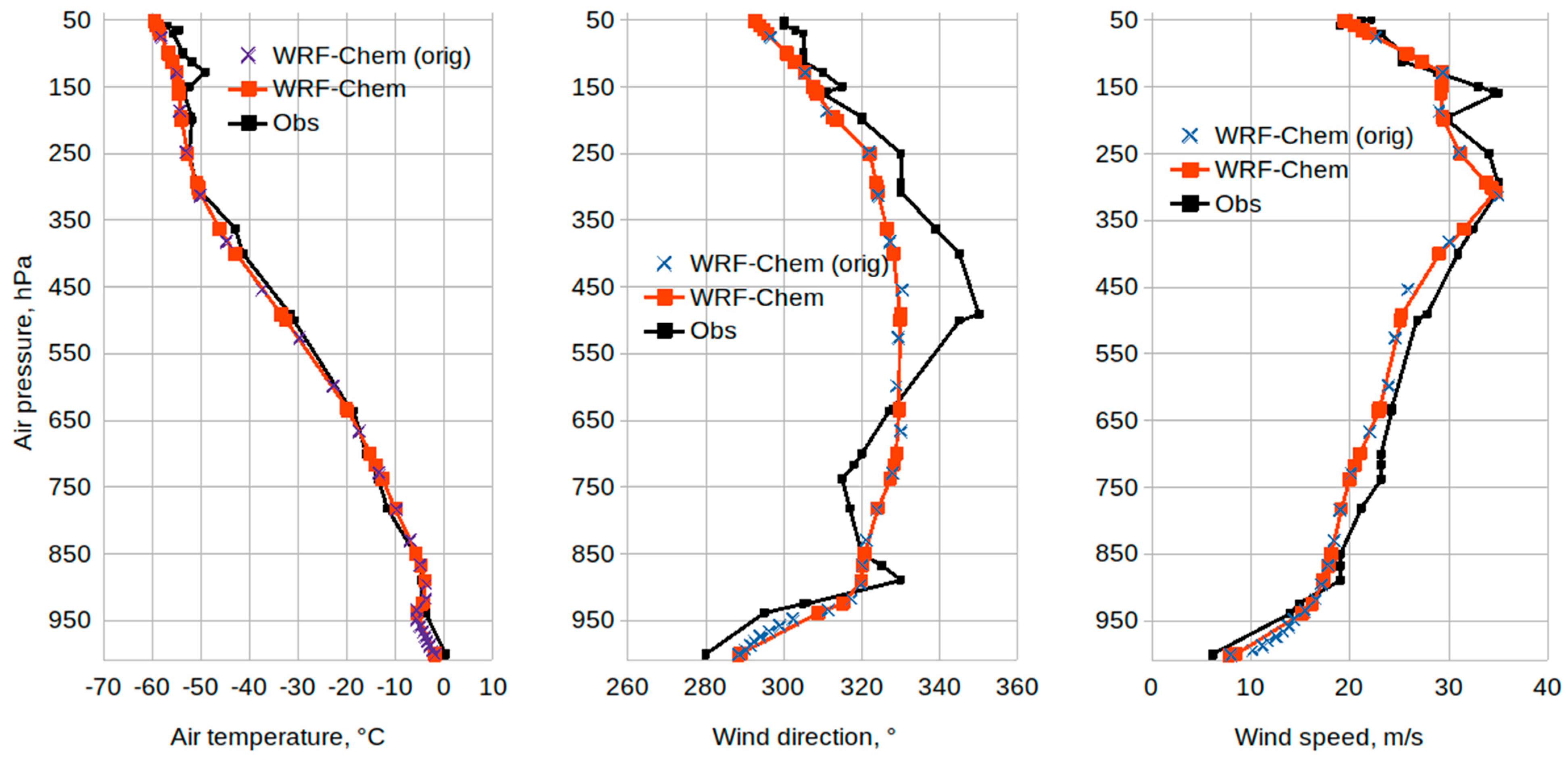
3.1.2. Vertical Distribution of Meteorological Parameters near St. Petersburg

The WRF-Chem model simulates the vertical profiles of three meteorological parameters—wind speed, direction and air temperature—in the troposphere and lower stratosphere above Voeikovo for January 2019–March 2020 relatively well. The distributions of these profiles by the modelling and measurements are presented in Figure A2 (Appendix C). In general, the shapes of three meteorological-parameter distributions determined by the modelling and radiosonde observations are quite similar. It can be seen that in the troposphere and lower stratosphere near St. Petersburg, eastward atmospheric transport (Figure A2a) with 4–10 m/s wind speed (Figure A2b) and 50–60 °C and 0–10 °C air temperature ranges (Figure A2c) are predominant.
The best fit between the modelling and measurement data is for air temperature, with MD = 0.4 °C, SDD = 2.5 °C and CC = 0.99. MD and SDD for wind speed are 0.5 and 4.1 m/s and 12.1 and 28.3° for wind direction, respectively. In the upper troposphere, the wind speed arrived at by the measurements and modelling can reach 40–50 m/s. This explains the large SDD of the parameter. The CC for the wind speed and direction are 0.93 and 0.86, respectively.
According to the analysis, the WRF-Chem model can probably be used to simulate horizontal and vertical distribution of the CO2 in the atmosphere. This will be the subject of our investigations in the next sections.

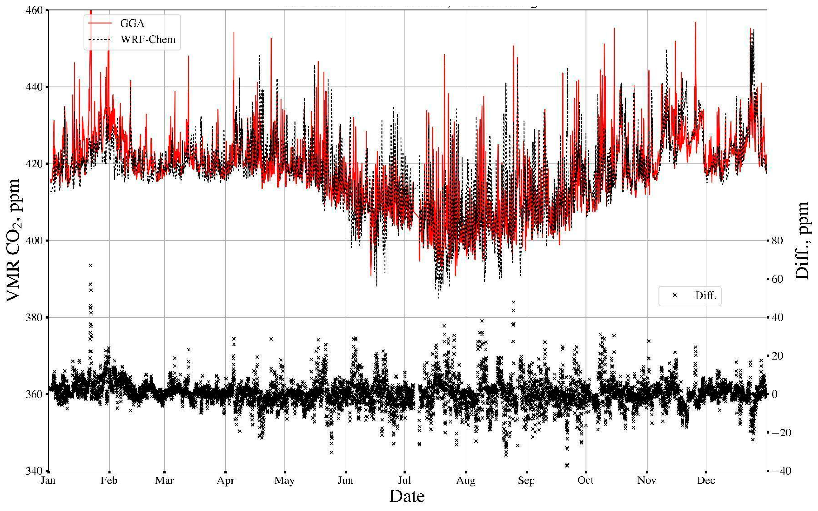
3.1.3. Near-Surface CO2 Mixing Ratio in Helsinki

Figure 8 depicts a time series of hourly averaged near-surface CO2 mixing ratios in Helsinki for 2019 according to the WRF-Chem simulation and the measurements. Table 3 presents the main characteristics of the discrepancies between the data. According to [62], a confidence interval of 95% confidence level is given for means
V M R C O 2 ¯ ± z S T D N [ p p m ] ,
where V M R C O 2 ¯ —mean near-surface CO2 mixing ratio (VMR—volume mixing ratio); z—quantile of normal distribution or Student coefficient for 95% confidence level; S T D —standard deviation from mean; N —size of a dataset.
The WRF-Chem model simulates well the temporal variation of the near-surface CO2 mixing ratio in Helsinki. The correlation is 0.73. MD and SDD are 0.15 and 1.68%, respectively. In general, the model underestimates the CO2 mixing ratio relative to the measurements.
From approximately April to October 2019, there was a clear influence from the vegetation season, which caused increases in the biogenic fluxes of CO2; this was registered by the measurements and modelling data and can be seen in Figure 8. Nevertheless, the WRF-Chem model underestimates the CO2 mixing ratio during vegetation season by ~3 ppm.
Excluding the biogenic influence causes an increase in MD from 0.15 to 0.45%, but a slight decrease in SDD, from 1.68 to 1.56%. In addition, this leads to an increase in MD by ~0.2% from April to August. It is probable that the small change in MD, while excluding the biogenic factor, is related to the influence of biogenic activity via chemical BCs which also influence diurnal variation of the near-surface CO2 mixing ratio during vegetation season. If the analysis excludes anthropogenic CO2 emissions and biogenic fluxes inside the modelling domain d04, MD increases from 0.15 to 1.44%, and CC decreases from 0.73 to 0.69.
A total of ~59.6% (from 8500) of all MDs are less than 4.2 ppm (1%), 32.6% of MDs are higher than 4.2–12.5 ppm (~1–3%) and only 8% of all MDs are higher than 12.5 ppm (3%). There are only a few (9, or 0.1% of all MDs) large differences which constitute ~40–60 ppm (10–15%). It is probable that they can be called anomalies.
The analysis of the relation between the near-surface CO2 mixing ratio modelling error and errors in the modelling of near-surface wind speed in Helsinki has demonstrated that there is no explicit relation (CC = ~−0.1). However, using only CO2 mixing ratio modelling errors larger than 3% (~12.5 ppm), weak negative correlation with the wind speed modelling error was found (CC = −0.4, with a dataset size of 732 vs. 8500). If one uses CO2 mixing ratio modelling errors which are higher than 17 ppm, CC also increases to −0.48, but for a significantly reduced dataset (282 vs. 8500). It was found that change in the sign of the CO2 mixing ratio modelling error leads to the opposite sign of the wind speed modelling error. It is logical, since if the model overestimates the wind speed, it should underestimate near-surface CO2 mixing ratio. Therefore, it can be said that the largest modelling errors of the near-surface CO2 mixing ratio in Helsinki are related to the near-surface wind speed modelling errors.

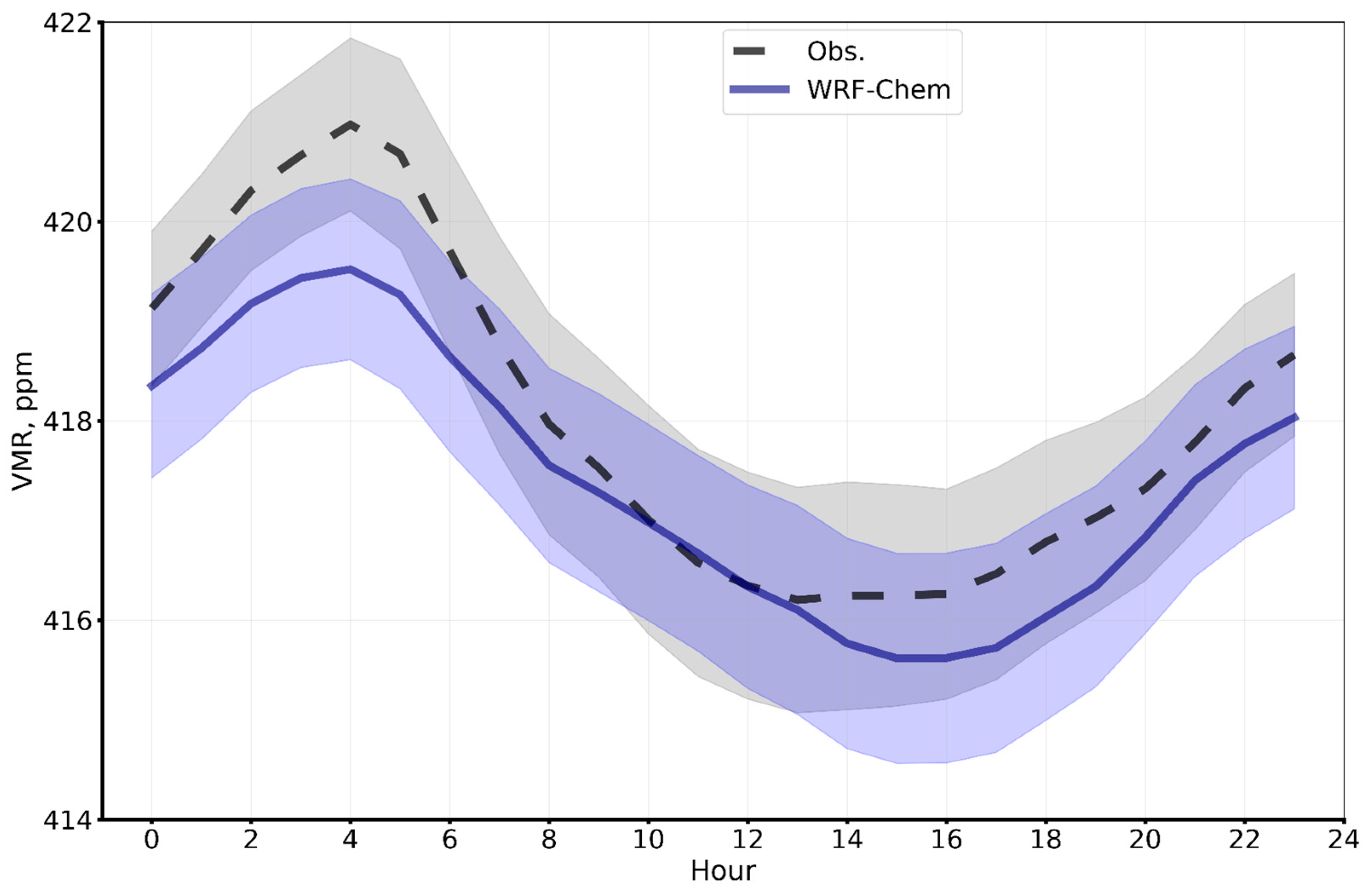
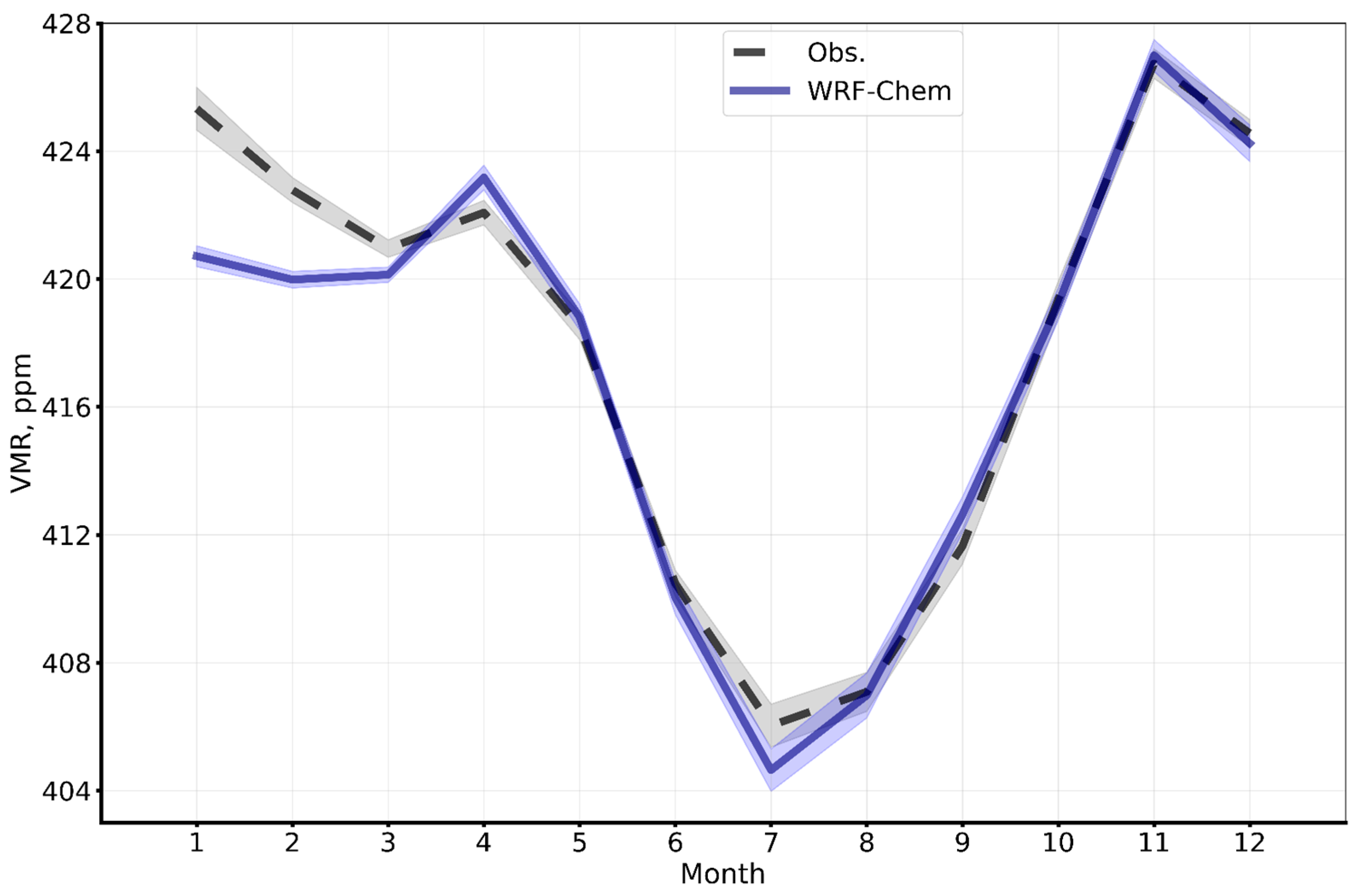
Modelling of Diurnal and Seasonal Variation of the Near-Surface CO2 Mixing Ratio

Figure 9 presents the mean diurnal variation of the near-surface CO2 mixing ratio at the measurement station in Helsinki for 2019, as determined by the WRF-Chem modelling and the measurements. The time is given in UTC. The shaded area shows confidence intervals.
In general, the WRF-Chem model simulates well the mean diurnal variation of the near-surface CO2 mixing ratio in Helsinki. The model underestimates the CO2 mixing ratio during night and day hours relative to the measurements by 1.5 ppm and less than 1 ppm, respectively. An analysis of the diurnal variation of near-surface wind speed together with CO2 mixing ratio was carried out. It demonstrated that the diurnal variation of the CO2 mixing ratio is probably influenced by biogenic CO2 fluxes during the vegetation season and clear diurnal variation of wind speed in spring and summer. It was found that the WRF-Chem model simulates low wind-speed conditions less accurately than high-speed conditions. This might be a reason for the lower CO2 mixing ratio during night hours determined by the WRF-Chem model [58,59]. In winter the diurnal variation of the CO2 mixing ratio in Helsinki is quite smooth, with an increase by 5 ppm to 12 UTC (according to the measurements). By contrast, in summer the diurnal variation of the mixing ratio is more pronounced, with a CO2 content variation of 10 ppm during the day. It is probable that the winter’s increase in atmospheric CO2 content is caused by the more frequent windless conditions and the larger number of air-temperature inversions. The worst fit between the modelled and measured mean diurnal variation of the CO2 mixing ratio is found for the winter season, and the best—for the spring. This could be caused by the larger errors in the modelling for near-surface wind speed during windless conditions. The confidence intervals for the observed and modelled data are quite similar, at ~±1 ppm, with an increase to 11–12 UTC.
An analysis of the variations of the near-surface CO2 mixing ratio during the week shows that both the WRF-Chem model and the measurements give a decrease in the mixing ratio by 1–1.5 ppm during weekends (Saturday and Sunday). This probably is related to the reduction of automobile traffic during the weekends and, as a result, to the decrease of anthropogenic CO2 emissions. However, the weekly variation of anthropogenic CO2 emissions was not set explicitly in the WRF-Chem model run. It is probable that the weekly variation of anthropogenic CO2 emissions was indirectly set via chemical BCs (CT-NRT.v2022-1) which were refreshed with a 6 h frequency. According to [63], in the framework of the CarbonTracker program, scaling factors are applied to fossil-fuel emissions. These factors characterise weekly and diurnal temporal variation of the emissions [64]. Hence, the weekly, and even diurnal, variation of CO2 atmospheric content due to anthropogenic activity was set in the WRF-Chem simulation via the boundaries of the d01 domain (Figure 2).
It can be seen from Figure 10 that the WRF-Chem model is able to simulate mean seasonal variation of the near-surface CO2 mixing ratio. Both the modelled data and the measurements show clear decreases of the CO2 mixing ratio from April to July, along with a subsequent increase. The amplitude of the change is 24 ppm (~5–6% from the mean measured value). The pronounced seasonal variation of the near-surface CO2 mixing ratio in Helsinki might be the consequence of plant activity during the vegetation season (~from the end of April to the end of September). During this period, plants start acting as the relatively large CO2 source during night hours and as a sink during daytime hours (see, for example, [36]). The largest differences between the main seasonal CO2 mixing ratios determined by the model and measurements in Helsinki are found in January–February (3–4 ppm). These can be caused by overestimation of near-surface wind speed in Helsinki by the WRF-Chem model, which is more significant during the winter season. On average, the confidence interval is ~0.5 ppm for both datasets.
Figure A3 of Appendix C demonstrates the spatial distribution of seasonally averaged near-surface CO2 mixing ratios (Figure A3a) and 10 m wind speed and direction (Figure A3b) as determined by the WRF-Chem modelling with an 8 km spatial resolution (domain d01) and by the ERA5 meteorological reanalysis (Figure A3c) for 2019. Note that the ERA5 reanalysis data are used in the WRF-Chem simulation as meteorological BCs.
At first, a pronounced CO2 seasonal variation can be seen in Figure A3a. The CO2 mixing ratio significantly decreases from spring to summer (on average, by 15–20 ppm). Then, from summer to autumn, the amount of CO2 starts to increase and does not significantly change from autumn to winter. Two main sources of CO2 which determine the local maximums of the CO2 mixing ratio are clearly seen, associated with the values higher than 450 ppm. These are anthropogenic emissions from the territories of the cities of St. Petersburg and Kirishi (Leningrad region). The source of CO2 in Kirishi might be a state regional power plant which is one of the largest power plants in the northwest part of Russia [65].
The mean wind speed and direction on average vary significantly from season to season. According to the modelling data, the largest near-surface wind speed values are found in winter (up to 4–4.5 m/s), and the lowest—in spring (less than 1 m/s). The mean maximum and minimum values of wind speed in general occupy the southern part of the domain (see Figure A3b, spring and winter). In addition, it was found that there was a pronounced tendency of wind speed to increase from spring to winter. It is probable that the highest values of near-surface wind speed during colder seasons are related to the higher contrasts of air temperature above water and earth surfaces. Comparing Figure A3b,c and Figure 1, it can be seen that a small local area of relatively high wind speed values (to the northeast of St. Petersburg) spatially correlates with the area of lowest terrain height (<50 m above sea level).
Comparing the spatial distribution of the mean wind-speed determined by the WRF-Chem model and by ERA5 reanalysis (Figure A3b,c), a relatively good spatial correlation was found. However, in general, the WRF-Chem model over- and underestimates wind speed values relative to the ERA5 data. On average, both modelled datasets represent quite similar 10 m wind directions within the domain. In particular, this can be seen in autumn and winter, when, according to both datasets, there are 10 m winds, predominantly in the north and north-east directions.

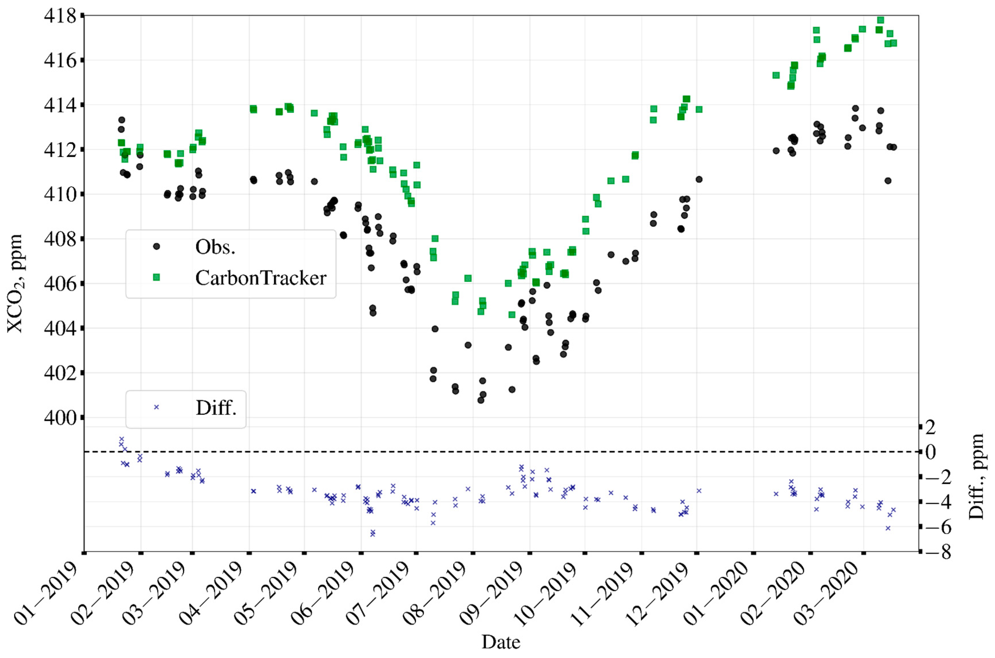
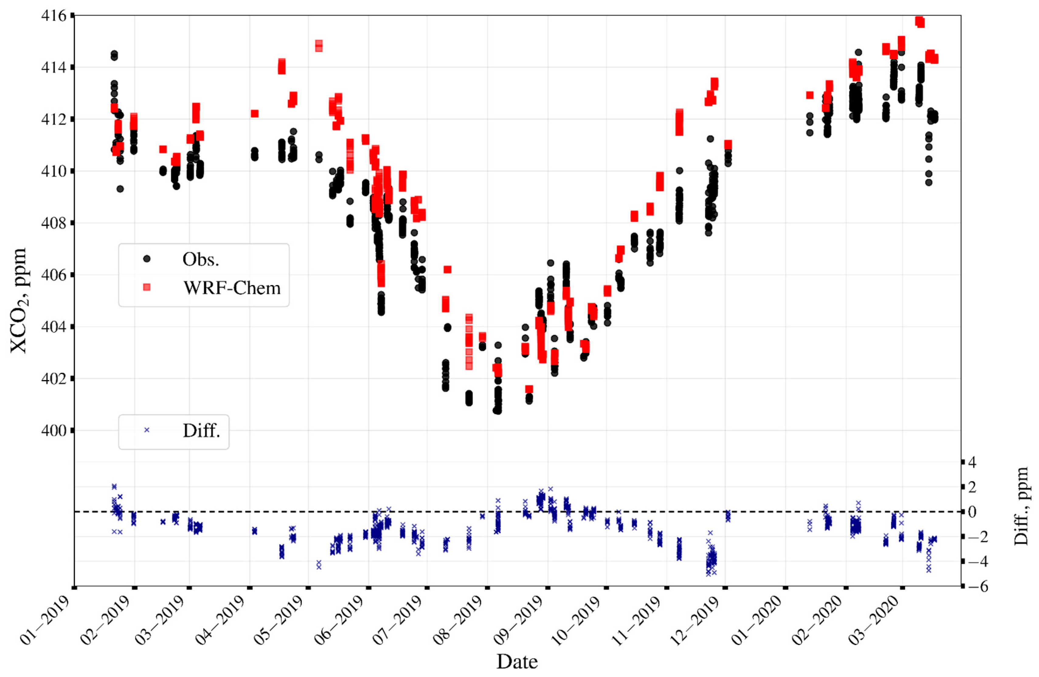
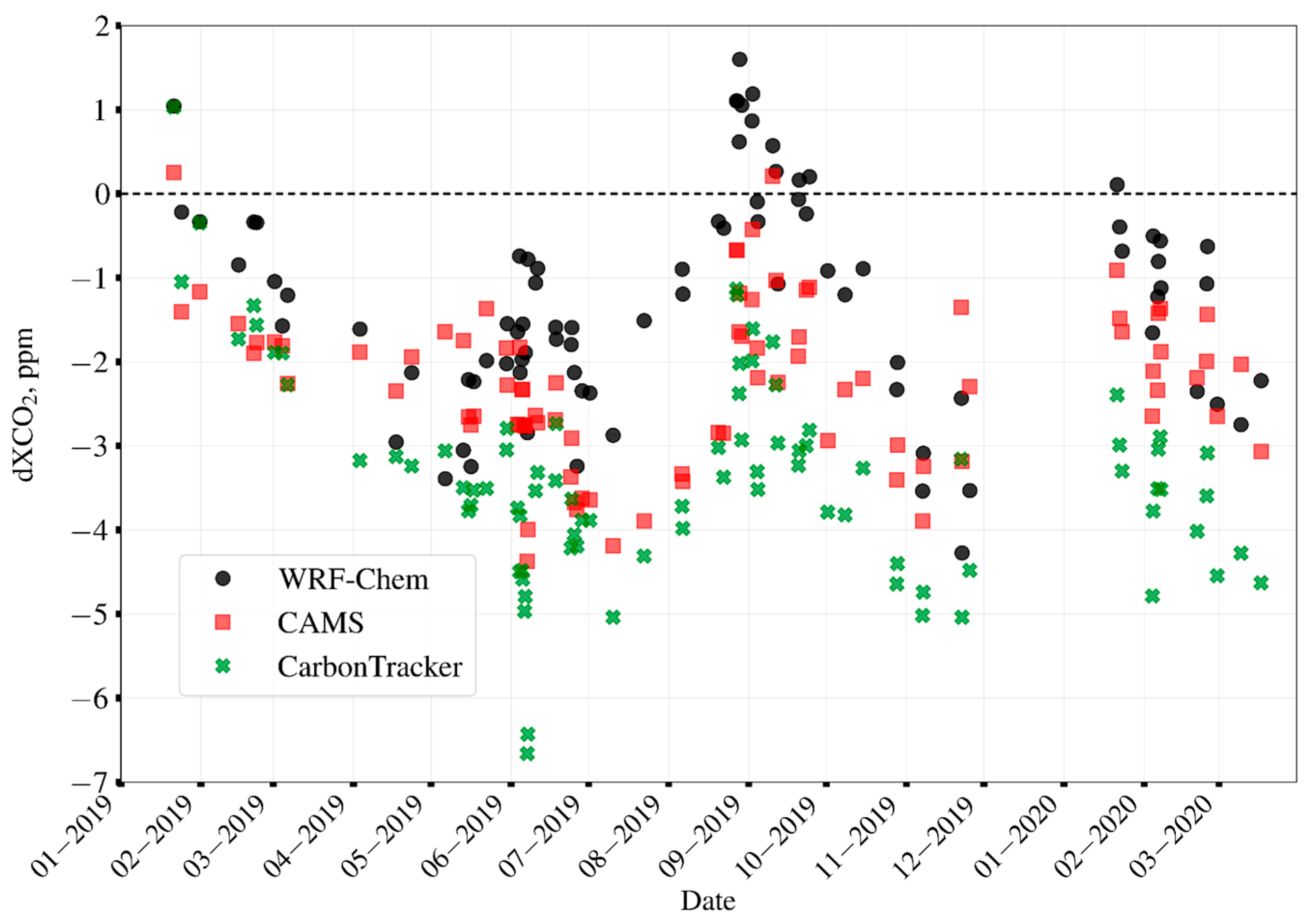
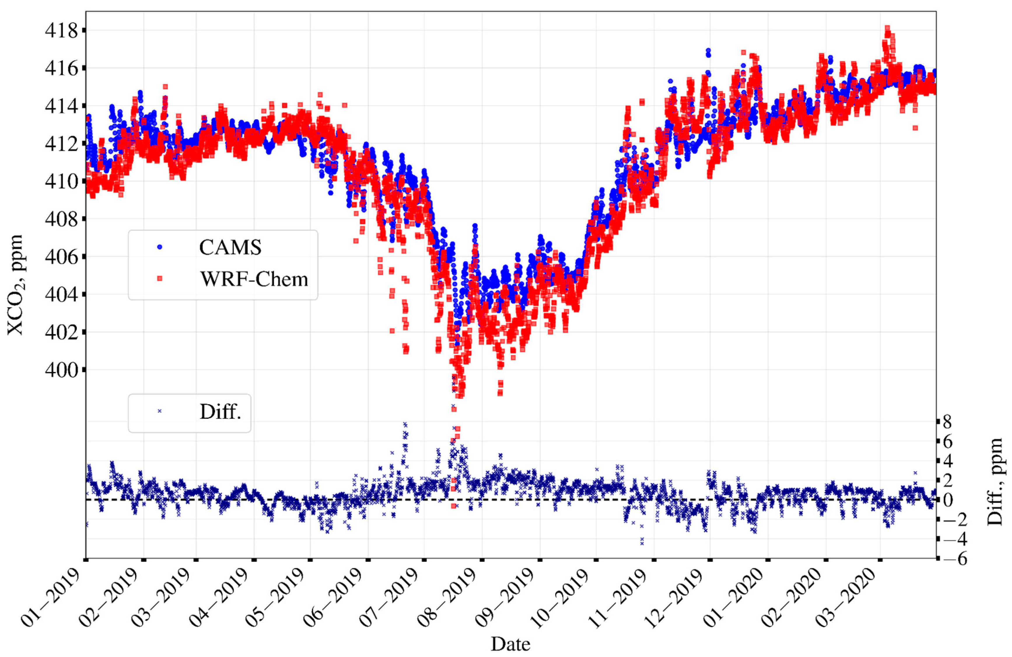
3.1.4. XCO2 in St. Petersburg

The time series of XCO2 determined by the WRF-Chem modelling and the measurements by the Bruker EM27/SUN in Helsinki are quite close to each other, with CC = 0.95 (Figure 11 and Table 4). The model simulates a decrease in XCO2 due to plant activity (approximately from May to October 2019), together with the subsequent increase, relatively well. In general, the modelled seasonal variation of XCO2 is influenced by transport from the boundaries of the modelling domain. In turn, the VPRM simulates local features of biogenic fluxes of CO2. MD and SDD between the modelled and measured data are −1.3 and 1.2 ppm, respectively (~0.3%). The MD can be caused by the errors in chemical BCs even though the BC correction was carried out. Note that the correction was based on the small dataset (14 pairs), which predominantly covers the winter season and does not reflect how the CarbonTracker data differ from the measurements obtained in other seasons of 2019. If chemical BCs are decreased by 0.3%, the MD also decreases to ~0%. However, such a correction cannot be provided without a solid argument (for instance, additional accurate measurements of XCO2).
In our previous study [22] a series of the WRF-Chem model runs with different settings were carried out to simulate CO2 transport in St. Petersburg for January 2019–March 2020. In particular, chemical BCs were set with more inaccuracies in the upper troposphere. Also, to calculate XCO2 using Equation (1), total water content measurements by a ground-based Bruker 125 HR in St. Petersburg were used. According to the results of [22], MD between the modelled and measured XCO2 constitutes 0.6%, which is about two times larger than the MD from the current study (Table 4). First, a worse fit between the modelled and measured XCO2 in St. Petersburg might be due to errors in the chemical BCs in the upper troposphere and lower stratosphere. Secondly, it can be caused by the use of a quite limited dataset of water vapour content in the atmosphere. For example, the dataset of water vapour content, as measured by the Bruker 125HR spectrometer, contains only 77 days of measurements in January 2019–March 2020. The current study has demonstrated that, by correctly setting chemical BCs and using modelled data of water vapour content in the atmosphere, it is possible to achieve better correspondence between the modelled and measured values of XCO2 in St. Petersburg.
In our estimation, three main factors determine the modelled XCO2—(1) atmospheric transport from the boundaries of the modelling domain, (2) anthropogenic CO2 emissions and (3) biogenic fluxes of CO2.
Table 5 presents a description of nine scenarios of the variations of modelled XCO2 components. Figure 12 depicts MDs (a) and SDDs (b) between XCO2 values in St. Petersburg for January 2019–March 2020 by the measurements and by WRF-Chem modelling. In addition, the figures show confidence intervals for every value.
As can be seen from Figure 12b, SDDs vary within the range of 0.30–0.33% (~0.1 ppm). This variation is quite small, and it can be assumed that none of the scenarios changes the SDD. Turning off the biogenic factor (Scenario 2) leads to an increase of MD by ~0.1% relative to the Control run (Scenario 1). Conversely, turning off the anthropogenic CO2 emissions causes an insignificant decrease of MD by 0.05%. It should be noted that MDs for the first five scenarios cover each other by confidence intervals. Therefore, they differ from each other insignificantly. The smallest MD is found for Scenario 6 (reduction of XCO2 from the chemical BCs by 0.3%). In addition, its confidence interval does not cover other MDs. Further reduction of XCO2 from the chemical BCs (Scenarios 7–9) leads to an almost linear increase of MDs.
Therefore, the MD between the modelled and measured XCO2 in St. Petersburg can be reduced to ~0% by an additional decrease in chemical BCs by 0.3%. However, SDD does not change significantly and still constitutes ~0.3%. It can be assumed that SDD is influenced by errors in a priori anthropogenic CO2 emissions and modelling of CO2 biogenic fluxes. The fact that turning off both of these factors does not reduce SDD probably means that there are inaccuracies in the spatial distribution of anthropogenic emissions, and in their diurnal, weekly, monthly variations.

3.2. XCO2 in St. Petersburg as determined by Independent Modelling

Due to the much cruder spatial resolution of the CAMS reanalysis relative to the WRF-Chem data, comparison was carried out for XCO2 only. For instance, in a prior study [66], the near-surface CO2 mixing ratio and XCO2 by CAMS reanalysis of the v18r3 version were compared to in situ and remote measurements in St. Petersburg (Peterhof) for 2018. It was shown that the differences between the modelled and measured near-surface CO2 mixing ratio significantly depended on the season, and vary by up to 3%. CC also depends on the month, varying from 0.26 to 0.81. However, that was expected, since near-surface CO2 mixing ratio is influenced by small-scale local processes which cannot be fully taken into account with a spatial resolution of more than 100 km.
The XCO2 time series in St. Petersburg for January 2019–March 2020 determined by CAMS and WRF-Chem fit with each other well (Figure A4 in Appendix C). MD and SDD are 0.15 and 0.3%, respectively, with a very high CC = 0.96. In general, the WRF-Chem data slightly underestimate XCO2 values relative to the CAMS reanalysis (positive difference). The maximum differences (up to 5 ppm) are found during the vegetation season. This probably means that biogenic fluxes of CO2 are treated differently in the models. In addition, XCO2 variation by the CAMS reanalysis is more smooth than that by the WRF-Chem model. It is probable that this is related to the cruder spatial resolution of the CAMS data.
Figure 13 depicts differences between XCO2 values determined by the Bruker EM27/SUN measurements and by the modelling (WRF-Chem, CAMS v21r2 and CarbonTracker v2022-1). The CAMS and CarbonTracker data are available with 3 and 6 h frequencies, respectively. Therefore, the minimum time step for the data comparison was 6 h. It can be summarised that the WRF-Chem-modelled data present XCO2 in St. Petersburg during the period of interest better than do the two other modelled datasets. MDs between the measurements and modelled data constitute 1.3, 2.3 and 3.3 ppm (0.3, 0.5 and 0.8%) for WRF-Chem, CAMS and CarbonTracker data, respectively. The SDDs are quite similar, at 0.2–0.3%. It is likely that the better agreement between the measurements and WRF-Chem data is related to the higher spatial resolution.

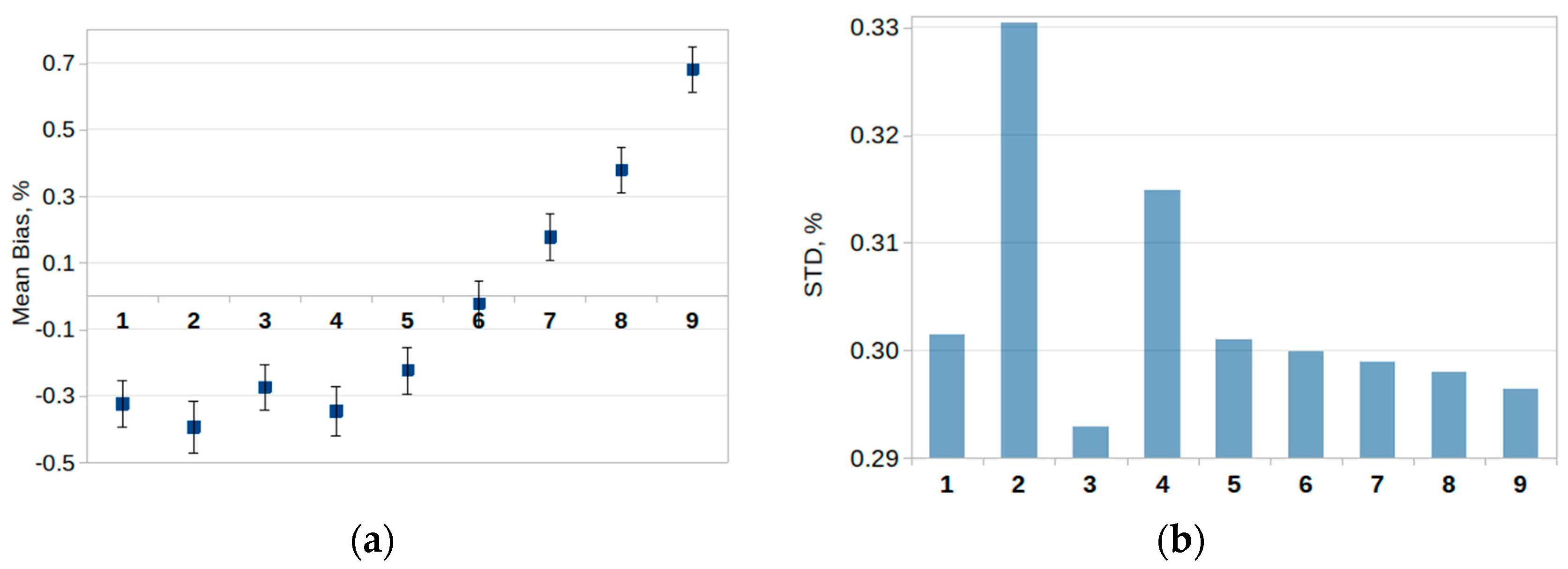
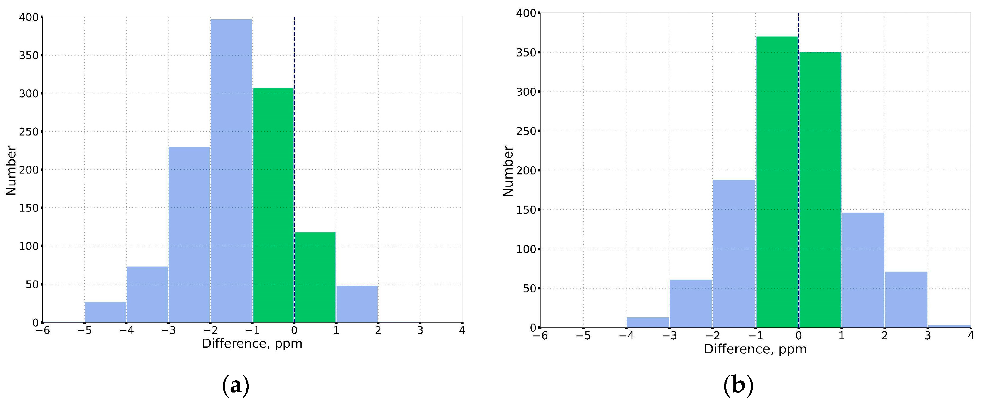
3.3. Compliance of XCO2 Modelling Errors with Modern Requirements

Today, there are many studies available which have assessed the ability of the WRF-Chem model to represent the near-surface concentration, vertical profile, and CO2 total column, from daily intervals to multi-year time intervals [18,19,22]. It is possible to achieve 0.1% or 0.5 ppm XCO2 modelling errors.
Prior studies [5,6] show that the anthropogenic contribution of St. Petersburg to the CO2 total column, as measured using paired high-precision spectrometers, ranges from less than 0.5 to 5 ppm. This characteristic is directly related to anthropogenic CO2 emissions from the city. The essence of paired measurements is the possibility of excluding all the main factors influencing the CO2 content except for anthropogenic emissions from the territory of the city under study. With this approach, taking into account the fact that the model qualitatively represents atmospheric transport, by varying the a priori anthropogenic emissions of the city, it is possible to achieve the best agreement between the modelling results and the measurements of XCO2.
However, if XCO2 measurements are available from only one instrument, then it is important to correctly take into account other influencing factors in the model (i.e., CO2 transfer from the boundaries of the modelling domain, contribution of plant activity, etc.). Therefore, with this approach, the permissible error of the modelling of CO2 content in the atmosphere depends on the magnitude of the anthropogenic contribution of a city. For example, if the anthropogenic contribution of a city to the total CO2 content according to measurements is 5 ppm, then, with a modelling error of 1 ppm, the systematic error of adjusted anthropogenic CO2 emissions will be 20%. If the contribution of a city according to measurements is 1 ppm, then, with the same modelling error, the systematic error of estimated emissions will be 100%.
Based on the range of the anthropogenic contribution of St. Petersburg to CO2 total atmospheric content from studies [5,6], it can be said that to assess the city’s anthropogenic emissions of CO2 using only one measuring instrument, the modelling error should be smaller than 1 ppm (0.2%).
Figure 14 shows histograms of the distribution of XCO2 modelling errors as determined by the WRF-Chem model for St. Petersburg for January 2019–March 2020. Figure 14a shows the differences between the measurements and original modelling data, and Figure 14b—the differences for the modelled data, with BCs reduced by 0.3% (scenario 6 from Table 5). The error ranges that can be considered as acceptable are highlighted in green (from −1 to 1 ppm).
The interval of acceptable differences in the case of the original WRF-Chem modelling (Figure 14a) covers ~35% (425) of all differences. The distribution of the differences seems to have a normal mode. The shift of the distribution to the left from a zero value indicates that the WRF-Chem overestimates the measured values of XCO2 in St. Petersburg due to systematic errors. These can be, for example, errors in chemical BCs. A decrease of chemical BCs by 0.3% (Figure 14b) moves the error distribution to the right. In this case, the interval of acceptable differences between the modelled and measured values of XCO2 covers ~60% of all differences.
It can be said that the use of the WRF-Chem model in estimating anthropogenic CO2 emissions from St. Petersburg requires careful validation, an example of which is given in the current study. First, based on a validation, the model will be adapted to the conditions of the modelling domain. Secondly, a validation allows for the filtering out of cases with the largest modelling errors. The current study has demonstrated that the WRF-Chem model, in ~60% of cases, can be used, together with high-precision measurements of total CO2 content, to estimate anthropogenic CO2 emissions for St. Petersburg for the period January 2019–March 2020.

4. Conclusions

In the current study, a complex validation of the WRF-Chem modelling of CO2 transport in the troposphere above the region of the Gulf of Finland, with focus on St. Petersburg and Helsinki, was carried out.
It is shown that by using the WRF-Chem model it is possible to simulate the annual variation of the near-surface CO2 mixing ratio and CO2 total columns (with additional data above 20 km). The model represents the mean seasonal and diurnal variation of atmospheric CO2 related to plants’ activity, and wind speed. The modelled and measured near-surface CO2 mixing ratio in Helsinki for 2019 correlates well (correlation coefficient is 0.73) with the mean difference and its standard deviation of 0.15 ± 0.04 and 1.7%, respectively.
The WRF-Chem model is able to simulate temporal variation of the column-averaged CO2 mixing ratio (XCO2) in St. Petersburg, characterising on average the total atmospheric column of CO2. A correlation coefficient between the modelled and measured (by ground-based Fourier–spectrometer Bruker EM27/SUN) time series of XCO2 is 0.95 with a mean difference and its standard deviation of ~−0.3 ± 0.02 and 0.3%, respectively. These estimates are in agreement with independent studies of other cities (e.g., Berlin, Saint-Denis). It is likely that the modelling errors are related to inaccuracies in chemical boundary conditions and, probably, the spatial distribution of a priori anthropogenic emissions of CO2.
XCO2 values in St. Petersburg, as derived by the WRF-Chem model, fit well with independent modelled data such as CAMS reanalysis and the CarbonTracker dataset. At the same time, the WRF-Chem data are in the best agreement with the measurements. It is probable that this is related to the much higher spatial resolution of the WRF-Chem modelling (2 vs. over 100 km), due to which local small-scale processes and high-resolution spatial distribution of a priori anthropogenic CO2 emissions can be considered in a simulation. This highlights the significance of numerical weather prediction and atmospheric composition models of high spatial resolution in estimating anthropogenic CO2 emissions on a city-wide scale.
The study has shown that by using the WRF-Chem model it is possible to simulate the dynamics of CO2 atmospheric content with a high spatial resolution (2 km). Following the recommendations given in this study, the modelling errors of XCO2 for St. Petersburg during January 2019–March 2020 are smaller than 0.2% in 60% of cases. We suppose that this is a requirement which should be fulfilled to estimate anthropogenic CO2 emissions on a city-wide scale for such megapolises as St. Petersburg.

Author Contributions

Conceptualization, G.N. and Y.T.; methodology, G.N., Y.T. and S.S.; software, G.N.; numerical modelling, G.N.; validation, G.N. and Y.T.; formal analysis, G.N., Y.T. and S.S.; investigation, G.N., Y.T. and S.S.; data curation, S.F. and A.P.; writing—original draft preparation, G.N. and Y.T.; writing—review and editing, G.N., Y.T., S.S., S.F., A.P. and M.S.; visualization, G.N. and M.S.; supervision, G.N. and Y.T.; funding acquisition, Y.T. and S.S. All authors have read and agreed to the published version of the manuscript.

Funding

Russian Science Foundation project, under the contract 23-77-30008.

Data Availability Statement

The simulation and measurements data are available upon request to [email protected].

Acknowledgments

Numerical experiments were performed using the computer cluster of the “Ozone Layer and Upper Atmosphere Research Laboratory” (O3Lab) of St. Petersburg University, and were partially covered by the Ministry of Science and Higher Education of the Russian Federation under the contract No 075-15-2021-583 and the state task for the Russian State Hydrometeorological University (project no. FSZU-2023-0004). The authors are grateful to the team of scientists from the National Oceanic and Atmospheric Administration (NCAR), the University Corporation for Atmospheric Research (UCAR), the National Oceanic and Atmospheric Administration (NOAA) and the Air Force (AFWA), USA, who developed, are developing, and are distributing the numerical-data free-of-charge model WRF-Chem. Also, the authors would like to thank Frank Hase, Thomas Blumenstock and Carlos Alberti from the Karlsruhe Institute of Technology (Karlsruhe, Germany) for providing the IR–Fourier spectrometer Bruker EM27/SUN and for their help with measurements and retrieving CO2 TC in St. Petersburg (measurements were carried out in 2019–2020). In addition, we would like to thank the team of the Voeikov Main Geophysical Observatory for providing vertical profile measurements of meteorological parameters. The authors thank the resource centre of St. Petersburg State University “Geomodel” for providing measuring equipment. The authors are also grateful to scientists Tuomas Laurila, Juha Hatakka and Ivan Mammarella from the Finnish Meteorological Institute and the University of Helsinki for providing measurements of near-surface CO2 content and biogenic gas fluxes in Finland (the data were obtained in 2020). The authors would like to thank the NOAA ESRL science team for free access to CarbonTracker data (the data were obtained in 2021). Finally, the authors thank colleagues from the Max Planck Institute for Biogeochemistry (Jena, Germany) for their assistance with the VPRM model (communication during the period 2020–2021).

Conflicts of Interest

The authors declare no conflict of interest.

Appendix A. Accounting for CO2 Content above 20 km

As mentioned above, the WRF-Chem model considers only processes in the troposphere and lower stratosphere. By contrast, the ground-based spectroscopic measurements of CO2 TC in St. Petersburg cover the entire atmospheric column. This can artificially contribute to the XCO2 modelling error. In a prior study [22], Copernicus Atmosphere Monitoring Service (CAMS) reanalysis data of v21r2 version [37] were used to set CO2 content above ~20 km.
Note that the CAMS reanalysis overestimates XCO2 in St. Petersburg for January 2019–March 2020 by 2.2 ppm, or 0.5% relative to the Bruker EM27/SUN measurements. Therefore, these data were reduced by the corresponding magnitude before using them to calculate modelled XCO2.
Finally, XCO2 values determined by the WRF-Chem model were calculated as the following:
X C O 2   w r f = (   T C C O 2   w r f , < 20   k m + T C C O 2   C A M S , > 20   k m ) / ( T C a i r , w r f T C w a t e r , w r f ) 10 6 ,
T C C O 2   w r f , < 20   k m = i = 1 N Δ P i C O 2   i
where T C C O 2   w r f , < 20   k m amount of CO2 molecules in a layer below ~20 km agl by the WRF-Chem modelling; T C C O 2   C A M S , > 20   k m amount of CO2 molecules in a layer above ~20 km agl by the CAMS reanalysis; T C a i r ,   w r f and T C w a t e r ,   w r f —amount of air and water molecules in the total atmospheric column; N —the number of WRF-Chem vertical levels; Δ P i —air pressure between layers i and i + 1 determined by the WRF-Chem modelling; C O 2   i —CO2 mixing ratio on a vertical layer i as determined by the WRF-Chem modelling.

Appendix B. Measurements of CO2 Fluxes by Vegetation at the SMEAR Station and Partial VPRM Optimisation

To optimise and validate the VPRM model, the measurements of air temperature, GPP (gross primary product; CO2 absorbed by vegetation) and NEE (net ecosystem exchange; difference between GPP and the product of plants’ respiration, or Resp) at the “SMEAR II Hyytiälä forest” station [26] are used in this study. The parameter Resp (CO2 emitted by vegetation) is calculated as the sum of NEE and GPP. At the Hyytiälä station, NEE and GPP measurements are carried out at a height of about 27 m (https://wiki.helsinki.fi/display/SMEAR/Eddy233 (accessed on 25 July 2021)). The assessment of GPP, Resp and NEE is based on a simple empirical model [67], and measurements of biogenic CO2 fluxes are taken using a set of instruments consisting of a Gill HS-50 ultrasonic anemometer measuring wind speed and temperature, and a Li-7200 gas analyser measuring CO2 and water vapour content [68,69]. The data is available at https://smear.avaa.csc.fi/download (accessed on 25 July 2021).
At Hyytiälä station, mast measurements are available at several heights of approximately 10 m, 20 m and above. We used the air temperature data closest to the Earth’s surface due to the fact that biogenic emissions of CO2 estimated by the VPRM are linearly related with near-surface air temperature. In addition, the analysis showed that the air temperature at an altitude of about 27 m, based on measurements at the Hyytiälä station, differs from the temperature at an altitude of 1.5 m by an average of ~3% and has a correlation of ~0.99. GPP, Resp and NEE are obtained using the turbulent pulsation method.
Table A1. VPRM parameters “a” and “b” for a vegetation type “mixed forest” before and after optimization.
ParametersBefore CorrectionAfter Correction
a0.17971.4650
b0.88001.4650

Appendix C

Figure A1. Time series of GEE (a) and Resp (b) according to WRF-Chem modelling and measurements at the “SMEAR II Hyytiälä forest” station in Finland for January 2019–March 2020; GEE—gross ecosystem exchange; Resp—respiration.
Remotesensing 15 05757 g0a1
Figure A2. Histograms of the distribution of meteorological parameters’ vertical profiles ((a)—wind direction, (b)—wind speed, (c)—air temperature) for Voeikovo for January 2019–March 2020 by aerological measurements and the WRF-Chem modelling.
Remotesensing 15 05757 g0a2
Figure A3. Spatial distribution of seasonally averaged near-surface CO2 mixing ratio (a), 10 m wind speed and direction by the WRF-Chem model (b) and by the ERA5 reanalysis (c) for 2019. The frequency of arrows is chosen for representability only and does not characterise the spatial resolution of both datasets; from (top) to (bottom)—spring, summer, autumn, winter; blue circle—Peterhof, St. Petersburg; red square—Helsinki.
Remotesensing 15 05757 g0a3
Figure A4. Time series of XCO2 for St. Petersburg for January 2019–March 2020 as determined by the WRF-Chem modelling and CAMS v21r2 reanalysis, and their differences (“Diff”; CAMS-WRF-Chem, right scale).
Remotesensing 15 05757 g0a4

References

  1. Contribution of Working Group I to the Sixth Assessment Report of the Intergovernmental Panel on Climate Change. Masson-Delmotte, V., Zhai, P., Pirani, A., Connors, S.L., Péan, C., Berger, S., Caud, N., Chen, Y., Goldfarb, L., Gomis, M.I.; et al., Eds.; In Press. Available online: https://www.ipcc.ch/report/sixth-assessment-report-working-group-i/ (accessed on 11 February 2021).
  2. Methods for Remote Determination of CO2 Emissions. The MITRE Corporation JASON Program Office 7515 Colshire Drive McLean, Virginia 22102, 13 January 2011. Available online: https://irp.fas.org/agency/dod/jason/emissions.pdf (accessed on 13 February 2021).
  3. Oda, T.; Bun, R.; Kinakh, V.; Topylko, P.; Halushchak, M.; Marland, G.; Lauvaux, T.; Jonas, M.; Maksyutov, S.; Nahorski, Z.; et al. Errors and uncertainties in a gridded carbon dioxide emissions inventory. Mitig. Adapt. Strat. Glob. Chang. 2019, 24, 1007–1050. [Google Scholar] [CrossRef]
  4. Pillai, D.; Buchwitz, M.; Gerbig, C.; Koch, T.; Reuter, M.; Bovensmann, H.; Marshall, J.; Burrows, J.P. Tracking city CO2 emissions from space using a high-resolution inverse modelling approach: A case study for Berlin, Germany. Atmos. Meas. Tech. 2016, 16, 9591–9610. [Google Scholar] [CrossRef]
  5. Makarova, M.V.; Alberti, C.; Ionov, D.V.; Hase, F.; Foka, S.C.; Blumenstock, T.; Warneke, T.; Virolainen, Y.A.; Kostsov, V.S.; Frey, M.; et al. Emission Monitoring Mobile Experiment (EMME): An overview and first results of the St. Petersburg megacity campaign 2019. Atmos. Meas. Tech. 2021, 14, 1047–1073. [Google Scholar] [CrossRef]
  6. Ionov, D.V.; Makarova, M.V.; Hase, F.; Foka, S.C.; Kostsov, V.S.; Alberti, C.; Blumenstock, T.; Warneke, T.; Virolainen, Y.A. The CO2 integral emission by the megacity of St Petersburg as quantified from ground-based FTIR measurements combined with dispersion modelling. Atmos. Meas. Tech. 2021, 21, 10939–10963. [Google Scholar] [CrossRef]
  7. Enting, I.G. Inverse Problems in Atmospheric Constituent Transport; Cambridge University Press: Cambridge, UK, 2002; p. 392. [Google Scholar] [CrossRef]
  8. Nassar, R.; Jones, D.B.A.; Kulawik, S.S.; Worden, J.R.; Bowman, K.W.; Andres, R.J.; Suntharalingam, P.; Chen, J.M.; Brenninkmeijer, C.A.M.; Schuck, T.J.; et al. Inverse modeling of CO2 sources and sinks using satellite observations of CO2 from TES and surface flask measurements. Atmos. Meas. Tech. 2011, 11, 6029–6047. [Google Scholar] [CrossRef]
  9. Nassar, R.; Hill, T.G.; McLinden, C.A.; Wunch, D.; Jones, D.B.A.; Crisp, D. Quantifying CO2 Emissions From Individual Power Plants From Space. Geophys. Res. Lett. 2017, 44, 10045–10053. [Google Scholar] [CrossRef]
  10. Zheng, T.; Nassar, R.; Baxter, M. Estimating power plant CO2 emission using OCO-2 XCO2 and high resolution WRF-Chem simulations. Environ. Res. Lett. 2019, 14, 085001. [Google Scholar] [CrossRef]
  11. Shekhar, A.; Chen, J.; Paetzold, J.C.; Dietrich, F.; Zhao, X.; Bhattacharjee, S.; Ruisinger, V.; Wofsy, S.C. Anthropogenic CO2 emissions assessment of Nile Delta using XCO2 and SIF data from OCO-2 satellite. Environ. Res. Lett. 2020, 15, 095010. [Google Scholar] [CrossRef]
  12. Timofeyev, Y.M.; Nerobelov, G.M.; Virolainen, Y.A.; Poberovskii, A.V.; Foka, S.C. Estimates of CO2 Anthropogenic Emission from the Megacity St. Petersburg. Dokl. Earth Sci. 2020, 494, 753–756. [Google Scholar] [CrossRef]
  13. Timofeyev, Y.M.; Nerobelov, G.M.; Poberovskii, A.V. Experimental Estimates of Integral Anthropogenic CO2 Emissions in the City of St. Petersburg. Izv. Atmos. Ocean. Phys. 2022, 58, 237–245. [Google Scholar] [CrossRef]
  14. Houweling, S.; Aben, I.; Breon, F.-M.; Chevallier, F.; Deutscher, N.; Engelen, R.; Gerbig, C.; Griffith, D.; Hungershoefer, K.; Macatangay, R.; et al. The importance of transport model uncertainties for the estimation of CO2 sources and sinks using satellite measurements. Atmos. Meas. Tech. 2010, 10, 9981–9992. [Google Scholar] [CrossRef]
  15. Peylin, P.; Law, R.M.; Gurney, K.R.; Chevallier, F.; Jacobson, A.R.; Maki, T.; Niwa, Y.; Patra, P.K.; Peters, K.; Rayner, P.J.; et al. Global atmospheric carbon budget: Results from an ensemble of atmospheric CO2 inversions. Biogeosciences 2013, 10, 6699–6720. [Google Scholar] [CrossRef]
  16. Federal State Statistics Service. Available online: https://rosstat.gov.ru/ (accessed on 10 March 2021).
  17. Grell, G.A.; Peckham, S.E.; Schmitz, R.; McKeen, S.A.; Frost, G.; Skamarock, W.C.; Eder, B. Fully coupled ‘online’ chemistry in the WRF model. Atmos. Environ. 2005, 39, 6957–6976. [Google Scholar] [CrossRef]
  18. Callewaert, S.; Brioude, J.; Langerock, B.; Duflot, V.; Fonteyn, D.; Müller, J.-F.; Metzger, J.-M.; Hermans, C.; Kumps, N.; Ramonet, M.; et al. Analysis of CO2, CH4, and CO surface and column concentrations observed at Réunion Island by assessing WRF-Chem simulations. Atmos. Chem. Phys. 2022, 22, 7763–7792. [Google Scholar] [CrossRef]
  19. Zhao, X.; Marshall, J.; Hachinger, S.; Gerbig, C.; Frey, M.; Hase, F.; Chen, J. Analysis of total column CO2 and CH4 measurements in Berlin with WRF-GHG. Atmos. Chem. Phys. 2019, 19, 11279–11302. [Google Scholar] [CrossRef]
  20. Nerobelov, G.; Timofeyev, Y.; Smyshlyaev, S.; Foka, S.; Mammarella, I.; Virolainen, Y. Validation of WRF-Chem Model and CAMS Performance in Estimating Near-Surface Atmospheric CO2 Mixing Ratio in the Area of Saint Petersburg (Russia). Atmosphere 2021, 12, 387. [Google Scholar] [CrossRef]
  21. Foka, S.C.; Makarova, M.V.; Poberovsky, A.V.; Timofeev, Y.M. Temporal variations in CO2, CH4 and CO concentrations in Saint-Petersburg suburb (Peterhof). Opt. Atmos. I Okeana 2012, 32, 860–866. (In Russian) [Google Scholar]
  22. Nerobelov, G.M.; Timofeyev, Y.M.; Smyshlyaev, S.P.; Foka, S.C.; Imhasin, H.H. Comparison of CO2 Content in the Atmosphere of St. Petersburg According to Numerical Modeling and Observations. Izv. Atmos. Ocean. Phys. 2023, 59, 275–286. [Google Scholar] [CrossRef]
  23. Kempeneers, P.; Sedano, F.; Seebach, L.; Strobl, P.; San-Miguel-Ayanz, J. Data Fusion of Different Spatial Resolution Remote Sensing Images Applied to Forest-Type Mapping. IEEE Trans. Geosci. Remote Sens. 2011, 49, 4977–4986. [Google Scholar] [CrossRef]
  24. Center for Earth Observation and Modeling (CEOM). Available online: https://www.ceom.ou.edu/ (accessed on 11 April 2021).
  25. Kilkki, J.; Aalto, T.; Hatakka, J.; Portin, H.; Laurila, T. Atmospheric CO2 observations at Finnish urban and rural sites. Boreal Env. Res. 2015, 20, 227–242. [Google Scholar]
  26. Mammarella, I.; Kolari, P.; Vesala, T.; Rinne, J. Determining the contribution of vertical advection to the net ecosystem exchange at Hyytiälä forest, Finland. Tellus B Chem. Phys. Meteorol. 2007, 59, 900–909. [Google Scholar] [CrossRef]
  27. Available online: https://www.campbellsci.com.au/wxt536 (accessed on 11 April 2021).
  28. Hari, P.; Nikinmaa, E.; Pohja, T.; Siivola, E.; Bäck, J.; Vesala, T.; Kulmala, M. Station for Measuring Ecosystem-Atmosphere Relations: SMEAR. In Physical and Physiological Forest Ecology; Springer: Dordrecht, The Netherlands, 2013; pp. 471–487. [Google Scholar]
  29. List of SMEAR III Measurements. Available online: https://www.atm.helsinki.fi/smear/index.php/smear-iii/measurements (accessed on 11 April 2021).
  30. University of Wyoming, College of Engineering. Sounding Data. Available online: http://weather.uwyo.edu/upperair/sounding.html (accessed on 10 March 2021).
  31. Rella, C. Accurate Greenhouse Gas Measurements in Humid Gas Streams Using the Picarro G1301 Carbon Dioxide/Methane/Water Vapor Gas Analyzer. 2010 PICARRO, INC. Available online: http://www.cen-sun.com/ueditor/php/upload/file/20190806/1565079076987536.pdf (accessed on 21 July 2021).
  32. Frey, M.; Sha, M.K.; Hase, F.; Kiel, M.; Blumenstock, T.; Harig, R.; Surawicz, G.; Deutscher, N.M.; Shiomi, K.; Franklin, J.E.; et al. Building the COllaborative Carbon Column Observing Network (COCCON): Long-term stability and ensemble performance of the EM27/SUN Fourier transform spectrometer. Atmos. Meas. Tech. 2019, 12, 1513–1530. [Google Scholar] [CrossRef]
  33. Gisi, M.; Hase, F.; Dohe, S.; Blumenstock, T.; Simon, A.; Keens, A. XCO2-measurements with a tabletop FTS using solar absorption spectroscopy. Atmos. Meas. Tech. 2012, 5, 2969–2980. [Google Scholar] [CrossRef]
  34. Frey, M.; Hase, F.; Blumenstock, T.; Groß, J.; Kiel, M.; Mengis-tu Tsidu, G.; Schäfer, K.; Sha, M.K.; Orphal, J. Calibration and instrumental line shape characterization of a set of portable FTIR spectrometers for detecting greenhouse gas emissions. Atmos. Meas. Tech. 2015, 8, 3047–3057. [Google Scholar] [CrossRef]
  35. Alberti, C.; Tu, Q.; Hase, F.; Makarova, M.V.; Gribanov, K.; Foka, S.C.; Zakharov, V.; Blumenstock, T.; Buchwitz, M.; Diekmann, C.; et al. Investigation of spaceborne trace gas products over St Petersburg and Yekaterinburg, Russia, by using Collaborative Column Carbon Observing Network (COCCON) observations. Atmos. Meas. Tech. 2022, 15, 2199–2229. [Google Scholar] [CrossRef]
  36. Hu, X.-M.; Gourdji, S.M.; Davis, K.J.; Wang, Q.; Zhang, Y.; Xue, M.; Feng, S.; Moore, B.; Crowell, S.M.R. Implementation of improved parameterization of terrestrial flux in WRF-VPRM improves the simulation of nighttime CO2 peaks and a daytime CO2 band ahead of a cold front. J. Geophys. Res. Atmos. 2021, 126, e2020JD034362. [Google Scholar] [CrossRef]
  37. Chevallier, F.; Ciais, P.; Conway, T.J.; Aalto, T.; Anderson, B.E.; Bousquet, P.; Brunke, E.G.; Ciattaglia, L.; Esaki, Y.; Fröhlich, M.; et al. CO2 surface fluxes at grid point scale estimated from a global 21 year reanalysis of atmospheric measurements. J. Geophys. Res. Atmos. 2010, 115, D21307. [Google Scholar] [CrossRef]
  38. Skamarock, W.C.; Klemp, J.B.; Dudhia, J.; Gill, D.O.; Zhiquan, L.; Berner, J.; Wang, W.; Powers, J.G.; Duda, M.G.; Barker, D.M.; et al. A Description of the Advanced Research WRF Model Version 4.3 (No. NCAR/TN-556+STR). 2021. Available online: https://opensky.ucar.edu/islandora/object/opensky:2898 (accessed on 15 August 2021).
  39. Mlawer, E.J.; Taubman, S.J.; Brown, P.D.; Iacono, M.J.; Clough, S.A. Radiative transfer for inhomogeneous atmospheres: RRTM, a validated correlated-k model for the longwave. J. Geophys. Res. Atmos. 1997, 102, 16663–16682. [Google Scholar] [CrossRef]
  40. Dudhia, J. Numerical Study of Convection Observed during the Winter Monsoon Experiment Using a Mesoscale Two-Dimensional Model. J. Atmos. Sci. 1989, 46, 3077–3107. [Google Scholar] [CrossRef]
  41. Janjic Zavisa, I. The Step–Mountain Eta Coordinate Model: Further developments of the convection, viscous sublayer, and turbulence closure schemes. Mon. Wea. Rev. 1994, 122, 927–945. [Google Scholar] [CrossRef]
  42. Monin, A.S.; Obukhov, A.M. Basic laws of turbulent mixing in the surface layer of the atmosphere. Contrib. Geophys. Inst. Acad. Sci. USSR 1954, 151, 163–187. [Google Scholar]
  43. Janjic Zavisa, I. The surface layer in the NCEP Eta Model. In Proceedings of the Eleventh Conference on Numerical Weather Prediction, Norfolk, VA, USA, 19–23 August 1996; American Meteorological Society: Boston, MA, USA, 1996; pp. 354–355. [Google Scholar]
  44. Chen, F.; Dudhia, J. Coupling an Advanced Land Surface-Hydrology Model with the Penn State-NCAR MM5 Modeling System. Part I: Model Implementation and Sensitivity. Mon. Wea. Rev. 2001, 129, 569–585. [Google Scholar] [CrossRef]
  45. Grell Georg, A. Prognostic Evaluation of Assumptions Used by Cumulus Parameterizations. Mon. Wea. Rev. 1993, 121, 764–787. [Google Scholar] [CrossRef]
  46. Hong, S.-Y.; Lim, J.-O.J. The WRF single–moment 6–class microphysics scheme (WSM6). J. Korean Meteor. Soc. 2006, 42, 129–151. [Google Scholar]
  47. Salamanca, F.; Martilli, A. A new building energy model coupled with an urban canopy parameterization for urban climate simulations––Part II. Validation with one dimension off–line simulations. Theor. Appl. Climatol. 2010, 99, 345–356. [Google Scholar] [CrossRef]
  48. Hersbach, H.; Bell, B.; Berrisford, P.; Hirahara, S.; Horányi, A.; Muñoz-Sabater, J.; Nicolas, J.; Peubey, C.; Radu, R.; Schepers, D.; et al. The ERA5 global reanalysis. Q. J. R. Meteorol. Soc. 2020, 146, 1999–2049. [Google Scholar] [CrossRef]
  49. Hersbach, H.; Bell, B.; Berrisford, P.; Biavati, G.; Horányi, A.; Muñoz Sabater, J.; Nicolas, J.; Peubey, C.; Radu, R.; Rozum, I.; et al. ERA5 hourly data on single levels from 1959 to present. Copernicus Climate Change Service (C3S) Climate Data Store (CDS). 2018. Available online: https://cds.climate.copernicus.eu/cdsapp#!/dataset/reanalysis-era5-single-levels?tab=overview (accessed on 5 May 2021).
  50. Jacobson, A.R.; Schuldt, K.N.; Miller, J.B.; Tans, P.; Andrews, A.; Mund, J.; Aalto, T.; Bakwin, P.; Bergamaschi, P.; Biraud, S.C.; et al. CarbonTracker Near-Real Time, CT-NRT.v2020-1. NOAA Earth System Research Laboratory, Global Monitoring Division. 2020. Available online: https://gml.noaa.gov/ccgg/carbontracker/CT-NRT.v2020-1/ (accessed on 5 May 2021).
  51. Tomohiro, O.; Maksyutov, S. ODIAC Fossil Fuel CO2 Emissions Dataset (Version name: ODIAC2020b). Center for Global Environmental Research, National Institute for Environmental Studies. 2015. Available online: https://www.nies.go.jp/doi/10.17595/20170411.001-e.html (accessed on 15 May 2021).
  52. Böttcher, K.; Markkanen, T.; Thum, T.; Aalto, T.; Aurela, M.; Reick, C.H.; Kolari, P.; Arslan, A.N.; Pulliainen, J. Evaluating Biosphere Model Estimates of the Start of the Vegetation Active Season in Boreal Forests by Satellite Observations. Remote Sens. 2016, 8, 580. [Google Scholar] [CrossRef]
  53. Mahadevan, P.; Wofsy, S.C.; Matross, D.M.; Xiao, X.; Dunn, A.L.; Lin, J.C.; Gerbig, C.; Munger, J.W.; Chow, V.Y.; Gottlieb, E.W. A satellite-based biosphere parameterization for net ecosystem CO2 exchange: Vegetation Photosynthesis and Respiration Model (VPRM). Glob. Biogeochem. Cycles 2008, 22, GB2005. [Google Scholar] [CrossRef]
  54. Nerobelov, G.M.; Timofeyev, Y.M. Estimates of CO2 Emissions and Uptake by the Water Surface near St. Petersburg Megalopolis. Atmos. Ocean. Opt. 2021, 34, 422–427. [Google Scholar] [CrossRef]
  55. Nikitenko, A.A.; Nerobelov, G.M.; Timofeyev, Y.M.; Poberovskii, A.V. Analysis of ground-based spectroscopic measurements of CO2 in Peterhof. Sovrem. Probl. Distantsionnogo Zondirovaniya Zemli Iz Kosmosa 2021, 18, 265–272. (In Russian) [Google Scholar] [CrossRef]
  56. Evaluation and Quality Control document for observation-based CO2 flux estimates for the period 1979–2021, v21r1 Version 2.0. Available online: https://atmosphere.copernicus.eu (accessed on 10 June 2021).
  57. Mues, A.; Lauer, A.; Lupascu, A.; Rupakheti, M.; Kuik, F.; Lawrence, M.G. WRF and WRF-Chem v3.5.1 simulations of meteorology and black carbon concentrations in the Kathmandu Valley. Geosci. Model Dev. 2018, 11, 2067–2091. [Google Scholar] [CrossRef]
  58. Li, H.; Claremar, B.; Wu, L.; Hallgren, C.; Körnich, H.; Ivanell, S.; Sahlée, E. A sensitivity study of the WRF model in offshore wind modeling over the Baltic Sea. Geosci. Front. 2021, 12, 101229. [Google Scholar] [CrossRef]
  59. Miller, S.T.K.; Keim, B.D.; Talbot, R.W.; Mao, H. Sea breeze: Structure, forecasting, and impacts. Rev. Geophys. 2003, 41, 1011. [Google Scholar] [CrossRef]
  60. Lauvaux, T.; Miles, N.L.; Richardson, S.J.; Deng, A.; Stauffer, D.R.; Davis, K.J.; Jacobson, G.; Rella, C.; Calonder, G.-P.; DeCola, P.L. Urban Emissions of CO2 from Davos, Switzerland: The First Real-Time Monitoring System Using an Atmospheric Inversion Technique. J. Appl. Meteorol. Climatol. 2013, 52, 2654–2668. [Google Scholar] [CrossRef]
  61. Shu, Z.R.; Li, Q.S.; Chan, P.W.; He, Y.C. Seasonal and diurnal variation of marine wind characteristics based on lidar measurements. Meteorol. Appl. 2020, 27, e1918. [Google Scholar] [CrossRef]
  62. Dekking, F.M.; Kraaikamp, C.; Lopuhaä, H.P.; Meester, L.E. A Modern Introduction to Probability and Statistics; Springer Texts in Statistics; Springer: Cham, Switzerland, 2005. [Google Scholar] [CrossRef]
  63. CarbonTracker Documentation CT2022 Release. Available online: https://gml.noaa.gov/ccgg/carbontracker/documentation.php#tth_sEc4.1 (accessed on 12 June 2022).
  64. Nassar, R.; Napier-Linton, L.; Gurney, K.R.; Andres, R.J.; Oda, T.; Vogel, F.R.; Deng, F. Improving the temporal and spatial distribution of CO2 emissions from global fossil fuel emission data sets. J. Geophys. Res. Atmos. 2013, 118, 917–933. [Google Scholar] [CrossRef]
  65. Annual Report of Public Joint Stock Company of Generating Companies of the Wholesale Electricity Market for 2021. Available online: https://www.ogk2.ru/upload/iblock/e9f/2fl5rq2ylzvtevw1dh2tf89187c9s0jc/2022_06_29_ogk_2_AR_RUS_spread_print.pdf (accessed on 10 July 2022).
  66. Nerobelov, G.M.; Timofeyev, Y.M.; Smyshlyaev, S.P.; Virolainen, Y.A.; Makarova, M.V.; Foka, S.C. Comparison of CAMS Data on CO2 with Measurements in Peterhof. Atmos. Ocean. Opt. 2021, 34, 689–694. [Google Scholar] [CrossRef]
  67. Kulmala, L.; Pumpanen, J.; Kolari, P.; Dengel, S.; Berninger, F.; Köster, K.; Matkala, L.; Vanhatalo, A.; Vesala, T.; Bäck, J. Inter-and intra-annual dynamics of photosynthesis differ between forest floor vegetation and tree canopy in a subarctic Scots pine stand. Agric. For. Meteorol. 2019, 271, 1–11. [Google Scholar] [CrossRef]
  68. Mammarella, I.; Launiainen, S.; Gronholm, T.; Keronen, P.; Pumpanen, J.; Rannik, Ü.; Vesala, T. Relative Humidity Effect on the High Frequency Attenuation of Water Vapor Flux Measured by a Closed-Path Eddy Covariance System. J. Atmos. Ocean. Technol. 2009, 26, 1856–1866. [Google Scholar] [CrossRef]
  69. Mammarella, I.; Peltola, O.; Nordbo, A.; Järvi, L.; Rannik, Ü. Quantifying the uncertainty of eddy covariance fluxes due to the use of different software packages and combinations of processing steps in two contrasting ecosystems. Atmos. Meas. Tech. 2016, 9, 4915–4933. [Google Scholar] [CrossRef]
Figure 1. Vertical profiles of air temperature, wind direction and speed (from left to right) in Voeikovo for 19 December 2019 12 UTC, by aerological observations and WRF-Chem modelling. “WRF-Chem orig”—WRF-Chem-modelled data before the interpolation to the observation vertical resolution; “WRF-Chem”—WRF-Chem-modelled data after the interpolation.
Remotesensing 15 05757 g001
Figure 2. WRF-Chem modelling domains; the symbols represent measurement stations—Peterhof, St. Petersburg (blue circle); Voeikovo (orange cross); Helsinki, Kumpula (red square); SMEAR II Hyytiälä (green rhombus). The colour of the map (from almost white to dark red) defines the terrain height relative to sea level in metres; a black dashed line contours the highest features of the terrain (<200 m).
Remotesensing 15 05757 g002
Figure 3. Spatial distribution of anthropogenic CO2 emissions from the territories of St. Petersburg (a) and Helsinki (b) for March 2019 according to the ODIAC inventory; locations of measurement stations in Peterhof and Kumpula are labelled with white circles; the territory of Helsinki is highlighted by a blue contour line.
Remotesensing 15 05757 g003
Figure 4. Time series of XCO2 in St. Petersburg for January 2019–March 2020 by Bruker EM27/SUN measurements and CarbonTracker v2022-1-modelled data and their differences (“Diff”; Obs—CarbonTracker, right scale).
Remotesensing 15 05757 g004
Figure 5. Histograms of the distribution of near-surface wind direction (a,b) and speed (c,d) in St. Petersburg (a,c) for January 2019–March 2020 and Helsinki (b,d) for 2019 as determined by measurements and WRF-Chem modelling.
Remotesensing 15 05757 g005
Figure 6. Mean diurnal variation of 10 m wind speed in St. Petersburg (a) and Helsinki (b) for 2019 as determined by the WRF-Chem modelling and measurements. Time is in UTC; the shaded areas are for confidence intervals at a 95% confidence level.
Remotesensing 15 05757 g006
Figure 7. Mean seasonal variation of 10 m wind speed in St. Petersburg (a) and Helsinki (b) for 2019 as determined by the WRF-Chem modelling and measurements. Time is local time; shaded areas are for confidence intervals at a 95% confidence level.
Remotesensing 15 05757 g007
Figure 8. Time series of near-surface CO2 mixing ratio in Helsinki in 2019 by the measurements and WRF-Chem modelling, as well as their differences (“Diff”; Observations minus WRF-Chem, right scale). GGA—greenhouse gas analyser (observations); VMR—volume mixing ratio.
Remotesensing 15 05757 g008
Figure 9. Mean diurnal variation of the near-surface CO2 mixing ratio in Helsinki for 2019 as determined by the WRF-Chem modelling and measurements; time is in UTC; shaded areas stand for confidence intervals at a 95% confidence level. VMR—volume mixing ratio; Obs.—observations.
Remotesensing 15 05757 g009
Figure 10. Mean seasonal variation of the near-surface CO2 mixing ratio in Helsinki for 2019 as determined by the WRF-Chem modelling and the measurements; shaded areas stand for confidence intervals of 95% confidence level. VMR—volume mixing ratio; Obs.—observations.
Remotesensing 15 05757 g010
Figure 11. Time series of XCO2 in St. Petersburg for January 2019–March 2020 by the WRF-Chem modelling and Bruker EM27/SUN measurements, and their difference (“Diff”; Observations minus WRF-Chem, right scale); Obs.—observations.
Remotesensing 15 05757 g011
Figure 12. MDs (a) and SDDs (b) between XCO2 as determined by the Bruker EM27/SUN measurements and WRF-Chem modelling for St. Petersburg for January 2019–March 2020, according to 9 scenarios; the description of the scenarios is in Table 5; values in % are given relative to the mean measured XCO2 value.
Remotesensing 15 05757 g012
Figure 13. Differences between measured (Bruker EM27/SUN) and modelled (WRF-Chem, CAMS v21r2, CarbonTracker v2022-1) XCO2 in St. Petersburg for January 2019–March 2020.
Remotesensing 15 05757 g013
Figure 14. A histogram of the error distribution of XCO2 modelling using the WRF-Chem model ((a)—XCO2 = XCO2 BC + XCO2 Ant + XCO2 Bio; (b)—XCO2 = XCO2 BC × 0.997 + XCO2 Ant + XCO2 Bio, see Table 5) for St. Petersburg for January 2019–March 2020.
Remotesensing 15 05757 g014
Table 1. The main parameters of WRF-Chem simulation. GHG—greenhouse gases; hor. res.—horizontal resolution.
ParameterDescription
Horizontal extent and resolutiond01 (800 × 800 km2)—8 km,
d02 (320 × 320 km2)—4 km,
d03 (110 × 110 km2, St. Petersburg)
and d04 (110 × 110 km2, Helsinki)—2 km
Vertical resolution25 hybrid levels,
from the surface up to 50 hPa
Initial and boundary conditionsMeteorologyERA5 reanalysis,
hor.res. 0.25°,
up to ~80 km on 137 hybrid levels
Atmospheric
CO2 content
CT-NRT.v2022-1,
hor.res. 2 × 3°,
up to ~200 km on 35 hybrid levels
CO2 sources and sinksAnthropogenic emissionsODIAC 2019,
hor.res. ~0.43 km2
Biogenic fluxesVPRM (online, every model time step);
Partially optimised by flux observations in Hyytiälä, Finland (see Appendix B);
Hor.res.—as in d01-d04,
Temporal resolution—8 days
Simulation periodJanuary 2019–March 2020, 10 min output
Chemistry optionGHG option: CO2 is treated
as a fully inert tracer
Table 2. Atmospheric processes and their parameterization schemes considered in the WRF-Chem model on a sub-grid scale.
ProcessScheme NameSource
Transfer of long-wave EM radiationin the atmosphereRRTM Longwave Scheme[39]
Transfer of short-wave EM radiationin the atmosphereDudhia Shortwave Scheme[40]
Earth’s boundary layer modelMellor–Yamada–Janjic[41]
Earth’s surface layer modelEta Similarity Scheme[42,43]
Model of land-surface layers’ interactionUnified Noah land-surface scheme for non-urban landcover surface energy fluxes[44]
Vertical transport and convective cloudsThe Grell 3D ensemble cumulus convection scheme[45]
Microphysics of cloudsWRF single-moment six-class schemes[46]
Urban effectBuilding Effect Parameterization (BEP)[47]
Table 3. Statistical characteristics of the differences between near-surface CO2 mixing ratios determined by the measurements and by WRF-Chem modelling for 2019; values in % are given relative to the mean measured value. STD—standard deviation from mean, MD—mean difference, SDD—STD of MD, CC—correlation coefficient, GGA—greenhouse gas analyser; a confidence interval at a 95% confidence level is given for means.
DataDataset SizeMean and STD, ppmMD and SDD,
ppm (%)
CC
GGA—WRF-Chem8565418.0 ± 0.2 and 9.7/
417.4 ± 0.2 and 9.5
0.6 ± 0.15 and 7.0
(0.15 ± 0.04 and 1.7)
0.73
Table 4. Statistical characteristics of the differences between XCO2 as determined by the Bruker EM27/SUN measurements and by WRF-Chem modelling, for January 2019–March 2020; values in % are given relative to the mean measured value; STD—standard deviation from mean, MD—mean difference, SDD—STD of MD, CC—correlation coefficient; a confidence interval of 95% confidence level is given for means.
DataMean and STD, ppmMD and SDD, ppm (%)CC
Bruker EM27/SUN—WRF-Chem408.4 ± 0.2 and 3.4/
409.7 ± 0.2 and 3.9
−1.3 ± 0.07 and 1.2
(−0.3 ± 0.02 and 0.3)
0.95
Table 5. Scenarios of variation of XCO2 components modelled by WRF-Chem. bio—biogenic influence; ant—anthropogenic influence; BCs—boundary conditions.
NNameDescription
1ControlControl WRF-Chem modelling
XCO2 = XCO2 BC + XCO2 Ant + XCO2 Bio
2No bioXCO2 = XCO2 BC + XCO2 Ant
3No antXCO2 = XCO2 BC + XCO2 Bio
4No bio and antXCO2 = XCO2 BC
5BCs reduced by 0.1%XCO2 = XCO2 BC × 0.999 + XCO2 Ant + XCO2 Bio
6BCs reduced by 0.3%XCO2 = XCO2 BC × 0.997 + XCO2 Ant + XCO2 Bio
7BCs reduced by 0.5%XCO2 = XCO2 BC × 0.995 + XCO2 Ant + XCO2 Bio
8BCs reduced by 0.7%XCO2 = XCO2 BC × 0.993 + XCO2 Ant + XCO2 Bio
9BCs reduced by 1.0%XCO2 = XCO2 BC × 0.990 + XCO2 Ant + XCO2 Bio
Disclaimer/Publisher’s Note: The statements, opinions and data contained in all publications are solely those of the individual author(s) and contributor(s) and not of MDPI and/or the editor(s). MDPI and/or the editor(s) disclaim responsibility for any injury to people or property resulting from any ideas, methods, instructions or products referred to in the content.

