
Your Input Matters—Comparing Real-Valued PolSAR Data Representations for CNN-Based Segmentation
by
 ,
,
Sylvia Hochstuhl
1,2,*,† ,
,
Niklas Pfeffer
1,2,†,
Antje Thiele
1,2,
Horst Hammer
2 and
Stefan Hinz
1 1
Institute of Photogrammetry and Remote Sensing, Karlsruhe Institute of Technology, 76131 Karlsruhe, Germany
2
Fraunhofer IOSB, 76275 Ettlingen, Germany
*
Author to whom correspondence should be addressed.
†
These authors contributed equally to this work.
Remote Sens. 2023, 15(24), 5738; https://doi.org/10.3390/rs15245738
Submission received: 17 September 2023
/
Revised: 30 November 2023
/
Accepted: 12 December 2023
/
Published: 15 December 2023
(This article belongs to the Section Remote Sensing Image Processing)
Abstract
:Inspired by the success of Convolutional Neural Network (CNN)-based deep learning methods for optical image segmentation, there is a growing interest in applying these methods to Polarimetric Synthetic Aperture Radar (PolSAR) data. However, effectively utilizing well-established real-valued CNNs for PolSAR image segmentation requires converting complex-valued data into real-valued representations. This paper presents a systematic comparison of 14 different real-valued representations used as CNN input in the literature. These representations encompass various approaches, including the use of coherency matrix elements, hand-crafted feature vectors, polarimetric features based on target decomposition, and combinations of these methods. The goal is to assess the impact of the choice of PolSAR data representation on segmentation performance and identify the most suitable representation. Four test configurations are employed to achieve this, involving different CNN architectures (U-Net with ResNet-18 or EfficientNet backbone) and PolSAR data acquired in different frequency bands (S- and L-band). The results emphasize the importance of selecting an appropriate real-valued representation for CNN-based PolSAR image segmentation. This study’s findings reveal that combining multiple polarimetric features can potentially enhance segmentation performance but does not consistently improve the results. Therefore, when employing this approach, careful feature selection becomes crucial. In contrast, using coherency matrix elements with amplitude and phase representation consistently achieves high segmentation performance across different test configurations. This representation emerges as one of the most suitable approaches for CNN-based PolSAR image segmentation. Notably, it outperforms the commonly used alternative approach of splitting the coherency matrix elements into real and imaginary parts.
1. Introduction
The ability to acquire information-rich image data of the earth’s surface regardless of cloud cover and daylight makes Polarimetric Synthetic Aperture Radar (PolSAR) systems important components in earth observation. The active sensors transmit and receive differently polarized microwaves, interacting with scatterers within the observed area. Analyzing the complex-valued measured signal, which is sensitive to the scatterers’ geometric form and geophysical parameters, enables a range of applications, including parameter retrieval (e.g., soil moisture [1,2] or surface roughness [3,4]) and the generation of land cover maps [5,6,7]. The task underlying the latter application is pixel-wise land cover classification, also known as PolSAR image segmentation, that is usually performed using supervised machine learning classifiers. A typical classification process involves the extraction of polarimetric features using target decomposition (e.g., eigenvalue decomposition or model-based decomposition [8,9,10,11,12,13]) and hand-crafted texture features (e.g., GLCM [14]). These features are subsequently used as input to machine learning classifiers such as Random Forest (RF) or Support Vector Machine (SVM) ([15,16,17,18]). In recent years, the application of deep learning models, particularly Convolutional Neural Networks (CNNs), for PolSAR image segmentation has been increasingly studied and has shown superior performance [19,20,21,22]. The main advantage of CNNs over shallow learning methods (such as RF and SVM) is that task-specific spatial image features are automatically learned during training, making the design of heuristic hand-crafted image features obsolete.
Different CNN architectures are used for PolSAR image segmentation, which is either pixel, patch, or image based. Pixel- and patch-based methods, proposed, for example, in [20,21], commonly apply CNN models, which consist of a sequence of convolutional and pooling filters followed by fully connected layers, to the entire image in a sliding-window fashion. In contrast, in image-based approaches, CNN models with an encoder–decoder structure, known as Fully Convolutional Networks (FCNs), incorporate a broader image context and allow the pixel-wise classification of large image patches within a single forward path. Several established FCN models, such as FCN-8/FCN-32 [23], U-Net [24], SegNet [25] or PSPNet [26], have been successfully adapted and applied for PolSAR image segmentation [5,27,28,29,30,31,32]. Complex-valued CNNs, as proposed in [33,34], have been developed to handle the complex-valued nature of PolSAR images effectively. These networks enable filtering, activation, and feature aggregation in the complex domain and demonstrate successful applications in the PolSAR segmentation. Despite their potential, complex-valued neural networks require additional resources compared to real-valued networks, due to the increased computational demands of complex arithmetic operations. This can lead to challenges in terms of training time and computational efficiency. Another challenge in the field of complex-valued CNNs is the limited research activity attributed to the predominant focus on real-valued neural networks in the broader machine learning community.
In contrast, real-valued CNNs have the advantage of being extensively studied and developed over the years, resulting in a wealth of research, techniques, and tools. It is necessary to convert the complex-valued data into a suitable real-valued representation to leverage the potential of this research advantage for PolSAR image analysis, including the use of established models and various optimization techniques. The choice of a real-valued representation that captures the essential information embedded in PolSAR data is not unique. This has resulted in using different representations used as CNN input in the existing literature. A commonly employed representation is derived directly from the spatially averaged coherency matrix that comprehensively describes the scattering processes statistically. In [35,36,37,38,39,40,41,42,43,44,45,46], a real-valued representation is constructed and used as a CNN input by concatenating the three real-valued diagonal entries with the real and imaginary components of the upper triangle entries into nine separate image channels. In contrast, Zhang et al. [47] propose representing complex-valued entries of the coherency matrix by their magnitude and phase. This approach aims to preserve the meaningful coupling between complex-valued data’s real and imaginary components. A further real-valued representation, frequently used as the CNN input [20,48,49,50,51,52,53], is the six-dimensional feature vector proposed in [20]. This representation, composed of the trace of the coherency matrix, two power-normalized diagonal elements, and three relative correlation coefficients, offers the advantage that five elements are normalized to a suitable value range of [0, 1]. To enhance the CNN-based segmentation, several studies [21,28,54,55] suggest incorporating domain and model-based knowledge regarding target scattering mechanisms by adding polarimetric features to the input layer.
The selection of a real-valued representation determines how well the information content of complex-valued data is preserved and presented to the CNN. Consequently, it is expected to influence the segmentation performance substantially. However, in the literature on CNN-based PolSAR image segmentation, this parameter is frequently neglected, and experiments often only employ a single, occasionally arbitrarily chosen, real-valued representation. The influence of the choice of the representation on segmentation performance has only been studied in a limited number of works, often in conjunction with other research objectives such as the development of new neural network architectures [21,56,57]. The current gap in the field lies in the absence of a comprehensive and systematic comparison of different PolSAR data representations in the context of CNN-based image segmentation. This knowledge gap may lead to the suboptimal performance and increased computational resources required for calculating and storing potentially unnecessary PolSAR features.
To fill this research gap, this study investigates the impact of the selected real-valued representations on the CNN-based PolSAR image segmentation performance. The primary objective of this research is to identify the most appropriate real-valued representation by conducting a comprehensive analysis of its influence on the segmentation performance across various CNN architectures. Specifically, this study investigates which of the following approaches for representing PolSAR data is the most suitable:
- The direct use of the coherency matrix elements represented by nine real values;
- The use of the six-dimensional feature vector proposed in [20];
- The use of physically interpretable features based on polarimetric target decomposition; or
- The use of a combination of coherency matrix elements and various polarimetric features.
The paper’s content is structured as follows: First, in Section 2, various real-valued PolSAR representations commonly used as the input for PolSAR segmentation in the literature are presented. These representations are then compared in the context of this study. Subsequently, in the same section, two distinct CNN architectures employed for PolSAR image segmentation in this study are introduced. Section 3 contains a detailed account of the experimental setup, including the data used for the experiments and the specific training strategy adopted for the CNN models. The results of the experiments are presented in Section 4 and subsequently discussed in Section 5. Finally, in Section 6, the conclusion of the study, summarizing the essential findings and their implications, is presented.
2. Methods
Different real-valued representations are chosen as the input for representative deep learning models to assess their impact on the performance of CNN-based PolSAR image segmentation. In the following section, the selected real-valued representations that have been used as input for CNN models in previous studies, along with their categorization, are presented. Subsequently, two specific CNN architectures are introduced that are employed in this study for PolSAR image segmentation.
2.1. Real-Valued PolSAR Data Representations
In general, the signal measured by a PolSAR system is represented by the complex-valued scattering matrix that describes the transformation, induced by observed scatterers, of the transmitted plane wave vector into the received plane wave vector :
According to the Backscattering Alignment convention, the backscattered signal is measured in the same polarization plane as the transmitted signal. Following this convention and assuming the commonly used monostatic configuration where the transmitter and receiver share the same antenna, the reciprocity theorem holds. This theorem dictates that for reciprocal scattering media, the equality holds true. The scattering matrix provides a complete characterization of deterministic (point-like) scatterers. However, in observing natural environments, multiple scatterers typically contribute to a single resolution cell, resulting in distributed scatterers. To describe this type of scattering behavior, a statistical formalism is required, which is represented by the averaged coherency matrix . This matrix is obtained by spatial or temporal averaging of the outer product of the scattering vector , which is derived from the vectorization of the scattering matrix using the Pauli basis:
Here denotes the complex conjugation and the matrix transpose. is a hermitian positive semi-definite matrix with real-valued power elements on the diagonal and complex-valued cross-correlations in the upper and lower triangle. Thus, the matrix is defined by nine real-valued parameters. is widely used as a comprehensive descriptor of distributed scattering phenomena, making it a common starting point for PolSAR image segmentation. However, to utilize real-valued CNNs for this task, the complex-valued matrix associated with each pixel needs to be transformed into a real-valued representation. This transformation can be achieved by either concatenating the nine independent real-valued parameters of , combining the entries into a feature vector, extracting physically interpretable features based on target decomposition methods, or employing a combination of these approaches. Table 1 provides an overview of various real-valued PolSAR data representations used as input for CNN models in the existing literature.
The first category, labeled as -elements, consists of representations derived directly from the coherency matrix . The most frequently utilized representation is called T9_real_imag, which is obtained by simply concatenating the real-valued diagonal elements and the real and imaginary parts of the upper triangle off-diagonal elements. In contrast, the equally computationally straightforward T9_amp_pha representation, which incorporates the amplitude and phase information of complex-valued elements, is less commonly used. This is despite the findings of [47], suggesting the potential of this representation for improved suitability in the CNN-based segmentation. To capture the significance of polarimetric phase differences, in this study, the representation T9_amp_pha is contrasted with T9_amp. The latter representation, used as CNN input in [58], solely considers the amplitude of the complex-valued elements.
The second category, labeled as -feature vector, is represented by the six-dimensional PolSAR data representation proposed in [20]. It is successfully used as an input for CNN models in several works [48,49,50,51,52,53]. The feature vector is composed of the total scattering power of all polarimetric channels in logarithmic scaling (), normalized power ratios ( and ) and relative correlation coefficients ():
According to [20], this representation is tailored explicitly for neural networks due to the constrained value range of power ratios and correlation coefficients. However, the superiority of this representation over the previously mentioned ones has not yet been analyzed.
The third category, labeled as Target decomposition, comprises representations based on physically interpretable polarimetric features extracted using coherent or incoherent target decomposition approaches. The Pauli representation is based on the coherent decomposition of the scattering matrix into matrices that correspond to a surface (), double-bounce (), or volume scattering () mechanisms:
The intensities , , and quantify the power scattered by the associated scattering mechanism. The Pauli decomposition is widely used to represent and visualize polarimetric information as a color image and is employed as CNN input in [31]. The analysis of the scattering matrix , which is only capable of characterizing deterministic scatterers, is insufficient to describe distributed scatterers accurately. Therefore, the analysis of a second-order descriptor, such as the coherency matrix, has to be considered. Model-based incoherent decomposition methods, such as the four-component Yamaguchi decomposition proposed in [10] and the three-component decomposition proposed in [60], are commonly employed to represent the coherency matrix as a combination of matrices corresponding to elementary scattering mechanisms. In this study, the resulting proportions of surface, double-bounce, and volume scattering obtained from these methods are combined into three-channel images, serving as input for CNNs. Further physically interpretable features that are frequently employed for land cover classification include entropy H, which measures the degree of randomness in the scattering process, mean alpha angle , which relates to the dominant scattering mechanism, and anisotropy A. These features are based on the eigenvalue decomposition of the coherency matrix proposed in [8]. An attempt to enhance the CNN-based PolSAR image segmentation using these features is described in [54].
Since representing PolSAR data with only three polarimetric features causes a loss of information, several researchers propose to combine multiple features to obtain a more comprehensive data description. These types of representations are assigned to the last category Combination in Table 1. To improve the performance of CNN-based segmentation, Gao et al. ([61]) propose a dual-branch network to combine the six-dimensional feature vector (Zhou) with Pauli decomposition parameters. Another combination is proposed in [62] that is composed of the amplitudes of the coherency matrix and scattering mechanism contributions according to the Yamaguchi decomposition. Chen and Tao [21] assemble the well-known features H, A, and the total scattering power () with so-called null angle features, which describe the target orientation diversity. The included null angle features, are defined as:
In [21], the ChenTao representation is compared to the T9_real_imag representation as an input for a patch-based CNN classification. It achieves slightly higher accuracies on two PolSAR datasets. To specifically investigate the usefulness of the two null angle parameters, the analysis presented here also includes a comparison to the representation based on the feature subset H_A__span. A further approach to combine polarimetric features within a CNN-based segmentation is proposed by Qin et al. in [56]. Their analysis identifies a suitable CNN input set of 16 components, which includes elements of , the smallest eigenvalue of , A and as well as . Adapting to that, this work includes the PolSAR data representation referred to as Qin in the investigation. Finally, a representation denoted as Mix is evaluated, which combines the ChenTao and Qin representations with the power of elementary scattering mechanisms based on the Yamaguchi decomposition. The Mix representation consists of 23 components, making it the most extensive representation in this comparison. Some of the extracted features, such as the amplitudes of elements in and scattering power contributions, exhibit distributions that deviate significantly from a normal distribution and possess a high dynamic range. These characteristics can potentially have a detrimental effect on the accuracy of segmentation, considering that CNNs are optimized for processing normally distributed RGB images. To mitigate this issue, the affected features are logarithmically scaled to approximate a normal distribution and reduce the dynamic range. Another crucial step in preprocessing is the standardization of features. This process converts the various feature values into a common unit, making them comparable. In image processing, z-standardization is typically employed, which involves subtracting the mean and dividing by the standard deviation. However, it is important to consider that the extracted PolSAR features may contain outliers, such as unusually high backscatter values caused by artificial structures. These outliers can greatly influence the mean and standard deviation, making z-standardization inadequate for achieving balanced feature scales. To address this issue, a robust standardization method based on the median and quantile range is employed:
where denotes the image data of component c, denotes the value of one pixel in , and and denote the 98th and 2nd percentiles of , respectively.
To form CNN input layers based on the selected real-valued representations, the corresponding scaled components are combined into a multi-channel image , where . Here, W and H represent the width and height of the image, and C represents the number of channels corresponding to the number of components in the representation.
It should be noted that concatenating the individual components into a multi-channel image deviates partially from the approach used in the cited works. The choice of the concatenation approach is motivated by its widespread use in the literature and its compatibility with established CNN models. Additionally, it ensures a fair comparison of the representations, as the same CNN architecture with an identical number of trainable parameters can be used for each representation.
2.2. CNN Segmentation Models
To analyze the suitability of the previously described PolSAR representations for CNN-based segmentation, two different CNN models are used, which are presented below. Both models are based on U-Net, a FCN introduced in [24] that consists of an encoding and a decoding path. The general structure of U-Net is visualized at the top of Figure 1. Within the encoder, contextual image features are extracted by the repeated application of convolution, activation, and aggregation. Thereby, the spatial dimension is reduced, while the feature dimension, which encodes the relevant image information, increases. Within the decoder, the resulting feature maps are gradually spatially up-sampled until the original spatial image dimension is reached, and a combination of convolution and softmax activation realizes a pixel-wise classification. To retain fine-scale spatial information, skip connections concatenate feature maps from the encoding path (blue) to up-sampled feature maps in the decoding path (grey).
As an encoder, an arbitrary CNN model can be used for feature extraction. Since the extracted features provide the basis for the final class separation, the choice of the CNN model significantly influences the segmentation result. In this work, two common models, a Residual Network (ResNet) proposed in [64] and an EfficientNet proposed in [65], are used as encoders. Both are visualized in Figure 1. ResNets are specific deep CNNs that are proven to be very powerful for the classification of RGB images. The high performance of this model has been achieved by introducing the concept of residual learning, which enables the training of very deep networks. Instead of direct mapping functions that transform an input into the desired output, residual functions are learned with reference to the layer inputs. This is realized using residual blocks (highlighted in orange in Figure 1). These contain so-called shortcut connections that perform an identity mapping of the input, which is added to the output of subsequent layers. In this work, ResNet-18, whose architecture is detailed in Figure 1, is used as the encoder of the U-Net model.
EfficientNet was proposed by Google in 2009 [65]. By scaling the network’s depth, width, and resolution in a structured way, good performance can be achieved with low resource consumption. The network is mainly built using mobile inverted bottleneck (MBConv) blocks introduced in [66] that are shown in Figure 1. This building block includes a so-called inverted residual block, which first employs point-wise convolution ( convolution) to project an input feature map into a higher dimensional space, subsequently performs depth-wise convolution, and finally projects the resulting feature map back to a lower dimensional space. The input feature map is added to the output feature map using a residual shortcut connection. The inverted residual block is extended by a Squeeze and Excitation (SE) block ([67]) consisting of a global pooling and two Fully Connected layers (FCs). This block allows the recalibration of channel-wise feature responses, which enables the network to provide higher weighting to relevant features. In this work, EfficientNet-b0, shown in Figure 1, is used as an encoder of the U-Net model.
In addition to the presented architectures, many other networks can be used as encoders, such as VGG, Inception, MobileNet, etc. ResNet-18 and EfficientNet-b0 were chosen as encoders in this work because they offer a good compromise between classification accuracy and the number of trainable parameters.
3. Experimental Setup
To identify the most suitable real-valued PolSAR data representation for the CNN-based segmentation, the two described CNN models are trained and tested using PolSAR data collected in two different frequency bands (S and L) taken from the Pol-InSAR-Island benchmark dataset [68]. Four test configurations are obtained by varying the CNN architecture and the frequency band used for data acquisition. This allows for evaluating the generalizability and robustness of individual representations against these variations. Additionally, the influence of the choice of data representation on the segmentation results compared to the effects of altering the CNN architecture or the frequency band can be assessed. The following presents the data used for training and testing the models and the applied training strategy.
3.1. Dataset
Commonly used benchmark datasets for PolSAR image segmentation include PolSF [69], the Flevoland AIRSAR dataset, and the Oberpfaffenhofen E-SAR dataset. However, these datasets have a significant drawback regarding the complexity of the segmentation tasks they provide. The Oberpfaffenhofen and PolSF datasets have very few generic classes, while the Flevoland dataset only includes rectangular cultivated crop fields, lacking diverse spatial arrangements of classes. Hence, high segmentation accuracies can already be achieved using simple classifiers. This limits the ability to compare sophisticated deep learning approaches. To address this limitation, in this paper, the recently published Pol-InSAR-Island dataset [68], which offers a more challenging segmentation task, is used for evaluation. The Pol-InSAR-Island dataset contains multi-frequency Pol-InSAR data acquired over the East Frisian island Baltrum by the airborne F-SAR system developed by the German Aerospace Center (DLR) [70]. The data, captured simultaneously in the L- and S-band, are provided as geocoded 6 × 6 Pol-InSAR coherency matrices on a 1 m × 1 m grid for each frequency band. Since this paper focuses on PolSAR image segmentation, only the upper left submatrix that represents the polarimetric coherency matrix of the master scene is used in our experiments. Before feature extraction, the image data are preprocessed using the Refined-Lee filter with a window size of to obtain averaged coherency matrices and suppress speckle noise.
The provided reference data yields pixel-wise labels of twelve predominantly natural land cover classes: Tidal flat (TF), Water (W), Coastal shrub (CS), Dense, high vegetation (DV), White dune (WD), Peat bog (PB), Grey dune (GD), Couch grass (CD), Upper salt marsh (US), Lower salt marsh (LS), Sand (S) and Settlement (SE). A visualization of the dataset is given in Figure 2. The dataset contains 5,450,807 labeled pixels, divided into spatially disjoint training and test data in roughly equal proportions. Table 2 shows the varying number of labeled pixels per class, which have to be taken into account during model training and testing.
In this study, the training data from the Pol-InSAR-Island dataset is divided into two subsets: one for supervised model training (training set) and the other for validating the model’s performance on unseen data during hyperparameter tuning (validation set). The training-to-validation data ratio is chosen as 3:1. The test data provided by the Pol-InSAR-Island dataset is exclusively used to evaluate the final models.
In order to enhance the robustness of the trained models and minimize overfitting, data augmentation techniques are employed to increase the amount of training data. This involves applying horizontal and vertical flipping and rotation by , or to image patches cropped from the training area.
3.2. Model Training
The evaluation of the considered PolSAR representations involves four different test configurations arising from using the two CNN models and separately evaluating S-band and L-band PolSAR image data. A model is trained, tuned, and tested for each data representation and test configuration following the setup described below.
During model training, validation, and testing, image patches with spatial dimensions of pixels are cropped from the training, validation, and test areas, respectively. It is worth noting that the class Peat bog is spatially concentrated within an area of approximately 300 m × 200 m. Therefore, larger patch sizes would result in insufficient patches encompassing this class. The batch size, representing the number of training patches processed within one training iteration, is set to 64. In this study, a thorough optimization of patch and batch size was not conducted, as the primary focus is not on model finetuning but rather on comparing different input data under the same training conditions.
Model training is conducted for a maximum of 100 epochs, with early termination after 30 epochs if no improvement in validation accuracy is observed. The learning rate, a crucial hyperparameter influencing training convergence, is adjusted using a dynamic approach based on the cosine annealed warm restart learning scheduler proposed in [71]. This approach reduces the learning rate following a cosine function. It includes multiple warm restarts, where the initial learning rate is decreased by a factor of 0.5 to avoid abrupt changes in training weights during advanced stages. Additionally, the number of training epochs until the following restart increases by a factor of 1.2. This work uses the implementation provided by [72]. The optimization of the training loss is performed using stochastic gradient descent (SGD) with a momentum of 0.9 and weight decay of 0.0005, following the proposed training strategy in [71].
In contrast to the standard approach in U-Net-based segmentation, this work utilizes the Focal Tversky Loss (FTL) proposed in [73] instead of the categorical cross-entropy loss. This decision is driven by the significant class imbalance observed in the training dataset, as shown in Table 2. Initial tests using a categorical cross-entropy loss revealed that the model disregards the underrepresented classes Peat bog and Dense, high vegetation after a few training epochs. Even a class-specific weighted categorical cross-entropy loss function did not lead to stable training results. The adoption of FTL is based on findings from a survey on loss functions for semantic segmentation conducted in [74]. FTL incorporates the Tversky similarity index, which quantifies the overlap between predicted and true classes and facilitates the balancing of False Positives (FP) and False Negatives (FN). The Tversky similarity index is defined as:
where p and g denote the predicted and true probabilities of a pixel i belonging to class c or . The hyperparameters and , which sum up to 1, determine the weighting between FP and FN samples in the Tversky similarity index. The constant prevents division by zero to ensure numeric stability. The FTL introduces a focal parameter to further allow the model to prioritize samples from underrepresented classes. The loss function is defined as:
While the FTL provides more stable training compared to categorical cross-entropy loss, the class Peat bog remains neglected. To address this, an additional weight factor of 1.8 is applied to pixels belonging to this class, determined through experimental testing. The choice of FTL hyperparameters and significantly impacts the segmentation results. Finding a single parameter set that maximizes segmentation accuracy across all data representations and model architectures is not feasible. To ensure a fair comparison between the representations, specific parameter sets are determined for each combination of data representation, model architecture, and frequency bands that achieve optimal results on the validation data. The tested values for are 0.3 and 0.6, and the tested values for are 0.5, 0.75, and 1.2. After selecting the optimal model parameters, the trained models are used to predict land cover classes for the test data, which were not used for training or validation.
4. Results
In the following, the results of the four test configurations: ResNet-U-Net on L-Band data, ResNet-U-Net on S-Band data, EfficientNet-U-Net on L-Band data, and EfficientNet-U-Net on S-Band data are presented. First, separate analyses are conducted for every test configuration. Subsequently, the results are summarized and considered collectively, enabling the identification of patterns and trends across the different test configurations. To quantify the segmentation results achieved on the test data, the Intersection-over-Union (IoU) is considered, which is a widely used metric for evaluating image segmentation results. It measures the overlap between the predicted segmentation mask and the reference mask. The formula for calculating IoU for one class i is given by:
where represents the number of correctly predicted pixels of class i, represents the number of pixels incorrectly predicted as class i, and represents the number of pixels of class i that were missed. The IoU ranges from 0 to 1, where 1 indicates a perfect overlap between the predicted and reference masks.
The mean IoU is used to evaluate multi-class segmentation. It is obtained by summing up the IoU for each class and dividing it by the total number of classes. The mean IoU is chosen for two reasons. Firstly, it provides a measure of the overall accuracy of the segmentation by considering both FP and FN. Secondly, it is robust to class imbalance in the test data.
4.1. ResNet-U-Net on L-Band Data
Figure 3 presents the segmentation results for L-band data obtained using the ResNet-U-Net model. The plot shows the mean IoU for each data representation used as input for the ResNet-U-Net model. The data representations on the y-axis are ordered based on their segmentation performance. The names of the data representations are color-coded according to their category in Table 1 (gray: -elements, pink: -feature vector, olive: Target decomposition, cyan: Combination).
The best performance, achieving a mean IoU of 82.73%, is obtained using the most extensive set of components called Mix, which comprises 23 components. The top five representations, each of which leads to a segmentation performance with mean IoU over 80%, also include Gao, Geng, T9_amp_pha, and H_A_α_span.
The success of using these data representations as input for the ResNet-U-Net model suggests that incorporating additional components contributes to improved segmentation performance. For example, the representation Mix outperforms Qin, Yamaguchi, and ChenTao, which are subsets of the component set used in Mix. Similarly, combining the representations Pauli and Zhou, referred to as Gao, yields better results than using either of them individually. The same applies to the representation Geng, which combines T9_amp and Yamaguchi.
However, the assumption that using more components always leads to better segmentation accuracy is contradicted by counterexamples. For instance, using the representation T9_amp_pha performs better than the representation Qin, which combines T9_amp_pha with additional components. Another interesting behavior is observed when comparing the three representations CP, H_A_α_span, and ChenTao. The three-channel representation CP, consisting of H, A, and , achieves a relatively low accuracy with a mean IoU of 74.09%. Adding the complementary component span (H_A_α_span) improves the segmentation accuracy by 6.67%. However, when the components and are also included (ChenTao), the mean IoU decreases to 74.79% (+0.7% compared to CP, −5.97% compared to H_A_alpha_span).
Another notable observation in the results is the poor performance when using the representation T9_real_imag. During the model training, it was observed that convergence could not be achieved within 100 epochs.
The class-wise mean IoU for each data representation is presented in Table 3 to provide a more detailed overview of the achieved results. The following description excludes the result of the non-converged model for T9_real_imag. In general, the classes Tidal flat, Water, and Sand are recognized with high accuracies, with mean IoU values greater than 90%, regardless of the chosen representation. The class Settlement is also identified with similarly high accuracies. Despite the limited availability of training data for the Peat bog class, it is reliably identified with IoU ranging from 79.40% to 96.43%. The most challenging task is distinguishing between Coastal shrub and Dense, high vegetation. This difficulty is suspected to arise from similar scattering mechanisms characterized by a high volume scattering component. The class White dune is completely ignored in the model predictions when using the representations T9_amp, Zhou, and ChenTao. The examination of predicted segmentation maps in Figure 4 reveals that image regions representing the White dune class are almost entirely assigned to the Grey dune class.
4.2. ResNet-U-Net on S-Band Data
In the following, the outcomes obtained by employing the same CNN architecture but varying the frequency band of the underlying data from the L-band (wavelength of about 20 cm) to the S-band (wavelength of about 10 cm) will be discussed.
Several observations can be made using the results presented in Figure 5. The ranking order of the representations remains similar to that observed in the L-band data results. The representations T9_amp_pha, Gao, and H_A_α_span continue to achieve high mean IoU, placing among the top performers. Further, the representations Zhou, CP, T9_amp, and T9_real_imag rank among the lower performers, with the latter failing to achieve model convergence during training.
However, a notable difference between L-band and S-band data segmentation is observed in segmentation accuracy when using the Mix representation. While it performs exceptionally well in classifying the L-band data, it only achieves a moderate ranking (8th place) when applied to the S-band data. This outcome further highlights that enriching input data with additional components, potentially containing supplementary information, does not guarantee an improvement in segmentation performance and may even lead to a degradation of results.
Examining the class-wise segmentation results in Table 4 provides further insights. Consistently with the previous findings, classes that are easily distinguishable, such as Tidal flat, Water, Sand, and Settlement, continue to exhibit minimal misclassifications. Challenges persist in accurately classifying the Coastal shrub and Dense, high vegetation classes. Furthermore, the representation ChenTao, T9_amp, and Zhou fail to detect the White dune class.
4.3. EfficientNet-U-Net on L-Band Data
In the following, the results obtained using EfficientNet as the encoder within the U-Net model are discussed. Changing the encoder results in learning different spatial features extracted from the provided data representations and used in the segmentation.
The results for L-band data are given in Figure 6 and Table 5. In the following, the results will be contrasted with the previously presented results obtained from the ResNet-U-Net segmentation for L-band data (Section 4.1).
Regarding the similarities, it is worth noting that the representation T9_real_imag once again fails to achieve model convergence during training. Furthermore, the representations Gao and T9_amp_pha consistently perform well, securing their positions among the top five representations. Another notable similarity is that the Pauli representation yields the best performance among the representations of the category Target decomposition. In terms of specific class separabilities, the classes Tidal flat, Water, Sand, and Settlement continue to be relatively easy to classify. In contrast, the classes Coastal shrub and Dense, high vegetation pose more significant challenges.
Considering the differences, the most significant change in achieved mean IoU is observed using the representation Mix. Applying the ResNet-U-Net architecture, the use of Mix ranks as the best-performing representation with a mean IoU of 82.73% (see Section 4.1). In contrast, using the EfficientNet-U-Net, it exhibits the third worst performance with a mean IoU of only 71.94%. The utilization of any representation that is a subset of the Mix representation, namely ChenTao, Qin and T9_amp_pha, leads to improved results. This further emphasizes that the combination of components, which, on the one hand, increases the information density but, on the other hand, also introduces redundancy in the data, can deteriorate the segmentation capability of the CNN. Alongside the observed degradation in segmentation performance for the Mix representation, there is a significant decrease of more than 4% in the segmentation performance for the Geng, VanZyl, and H_A_α_span representations. Conversely, significant performance increases are observed for T9_amp (+6.27%), Zhou (+6.03%) and ChenTao (+4.98%). Analyzing the class-wise results, a noteworthy difference is the successful recognition of the White dune class across all representations.
The key insight from comparing the results obtained using EfficientNet or ResNet as the backbone is that both the choice of architecture and the input representation strongly influence the segmentation performance. No clear favorite representation consistently outperforms others across the two models, nor does one favorable model consistently outperform the other regardless of the used PolSAR data representation as input.
4.4. EfficientNet-U-Net on S-Band Data
Investigating the segmentation results of this test configuration, given in Figure 7 and Table 6, the following observations can be made:
Similar to all other test configurations, the use of T9_real_imag does not converge during training, resulting in poor segmentation results on the test data. Another commonality is that T9_amp_pha consistently ranks within the top five performing representations, while the CP representation (here, second-worst mean IoU) falls within the bottom five. Additionally, the H_A_α_span representation (rank 2) and Qin (rank 3), which have already been among the top five representations in two other tests, prove to be suitable here as well.
A striking difference from other results is the notable performance improvement when using the VanZyl representation as input. In different test configurations, this data representation ranges in the middle or lower ranks (9, 9, 13), while in this particular test configuration, it achieves the best segmentation results. Regarding the class-specific results, it is noticeable that when using the Pauli representation, the class White dune is not predicted.
In general, the segmentation results obtained from the EfficientNet-U-Net are more influenced by changes in the frequency band compared to the results from the ResNet-U-Net. In contrast to the ResNet-U-Net tests, the ranking of the tested representations between S-band and L-band data significantly changes when utilizing the Efficient-U-Net.
4.5. Comprehensive Results Evaluation
The previous individual analyses of the results demonstrate that while the representation T9_real_imag consistently proves to be an unsuitable input for the applied CNN models, no data representation always delivers the best segmentation result across all tests. However, discernible trends and patterns can be observed, which will be discussed in the following. Figure 8 provides an overview of the mean IoU achieved by each data representation across all test configurations. It is intended to simplify the overall evaluation regarding the suitability of the tested data representations as an input for a CNN-based segmentation. For each representation, Figure 8 illustrates the range between the worst and best segmentation results, with the red marker indicating the mean value of the four test results. The representations are ordered on the y-axis based on their mean IoU averaged across the four test configurations.
Moving on to the specific results, the representation T9_amp_pha, which consistently ranks among the top 5 representations in all tests, achieves the best average result with 79.50% mean IoU. The representation Gao ranks second in this order. However, the poor performance in the fourth test (S-band image segmentation using EfficientNet-U-Net) leads to a relatively high range between the worst and best performance at 8.63%. Additionally, the minimal mean IoU achieved by Gao (73.56%) is lower than the minimal results obtained by the representations T9_amp_pha, Qin, and H_A_α_span. The Qin representation demonstrates the smallest variations in segmentation accuracy across the four test configurations, consistently achieving good results between 76.69% and 79.71%. Similarly, the H_A_α_span representation, which contains only four components, proves to be a suitable CNN input with accuracies between 76.58% and 80.76%. Among the representations that perform less favorably, with an average mean IoU of below 75% across the four test configurations, are Yamaguchi, T9_amp, Zhou, and CP.
The following examines the impact of incorporating individual components into a representation on segmentation performance. In certain instances, this leads to an increase in segmentation accuracy. Notably, the inclusion of the span component significantly enhances the performance of the initially subpar CP representation, resulting in the above-average performing H_A_α_span representation. The inferior performance using CP can be attributed to the absence of backscattering intensity information in this representation. Another example highlighting the impact of adding informative components to a representation on segmentation performance is the superior performance of T9_amp_pha compared to T9_amp. The two representations differ solely by including or excluding co- and cross-polar phase differences. It can be concluded that these phase differences provide valuable information for distinguishing different land cover classes, thereby enhancing segmentation accuracy. However, providing more information in the form of additional concatenated components as an input to the CNN does not directly lead to increased segmentation accuracy. This is evident from the results obtained using the most information-rich representation Mix. Utilizing subsets of this representation, namely Qin, T9_amp_pha, ChenTao, and H_A_α_span, leads to more stable and predominantly improved results.
To examine the influence of three factors (model architecture, frequency band, and data representation) on segmentation accuracy, a comparison is conducted by analyzing the differences between the maximum and minimum achieved accuracies under each factor variation. It is important to note that the T9_real_imag representation is excluded from this analysis.
Figure 9a focuses on the impact of the frequency band on segmentation results. It presents the difference in segmentation performance between L-band and S-band data for each data representation using a fixed CNN architecture. The ResNet-U-Net models (grey bars) generally exhibit less than 5% difference in IoU when comparing L-band and S-band data. However, the Mix representation shows a higher difference of 7.66%. The median difference is 1.95% (minimum 0.32%; maximum 7.66%). In contrast, when employing the EfficientNet-U-Net, larger differences in segmentation performance between L- and S-band data are observed, with a median difference of 6.32%, a minimum of 0.18%, and a maximum difference of 17.28%.
Figure 9b displays the difference in segmentation performance between the ResNet-U-Net and EfficientNet-U-Net models for each data representation, using the same frequency band. For L-band data, the median difference in mean IoU between the two models is 4.14% (minimum 1.05%; maximum 10.37%). When classifying S-band data, the median difference is slightly higher at 5.41% (minimum 1.19%; maximum 16.42%).
Figure 9c illustrates the difference between the highest and lowest results obtained when varying the data representation while keeping the model and frequency band constant. The differences are 11.37% (ResNet-U-Net, L-band), 11.29% (ResNet-U-Net, S-band), 7.93% (EfficientNet-U-Net, L-band), and 23.54% (EfficientNet-U-Net, S-band).
It is essential to interpret the difference values between the plots with caution. Plots (a) and (b) compare only two configurations (L-band and S-band, ResNet and EfficientNet), while plot (c) encompasses 13 different representations. Nevertheless, this analysis emphasizes that selecting an appropriate CNN architecture and frequency band is not the sole consideration in evaluating segmentation accuracy. Equally important is the thoughtful selection of a suitable representation for PolSAR data.
5. Discussion
To address the central question of how the selection of a real-valued representation of PolSAR data influences the segmentation performance using CNNs, 14 different representations used as CNN input were tested. The tests involved four configurations with varying CNN architectures (ResNet-U-Net and EfficientNet-U-Net) and frequency bands (S-band and L-band) of the underlying data. The results underscore the critical role of choosing a suitable representation of PolSAR data in developing the CNN-based segmentation. This is particularly evident through the differences in mean IoU values of 11.37%, 11.29%, 7.93%, and 23.54% obtained, which arise between the most suitable and the least suitable data representation for a fixed test configuration. While no representation consistently achieved the highest accuracy across all test configurations, a detailed analysis allows us to draw general conclusions about the different representation categories outlined in Section 1.
Among the representations belonging to the first category -elements, which directly represent the unique entries of the complex-valued coherency matrix using nine real values, are T9_real_imag and T9_amp_pha. The T9_real_imag representation consistently exhibited poor performance, failing to achieve model convergence during training and resulting in the worst segmentation results on test data. This can be attributed to separating the real and imaginary parts, which disrupts the essential relationship between them and leads to the loss of crucial information. Despite this plausible explanation, the finding is surprising, given the status of T9_real_imag as one of the most frequently used representations in the context of CNN-based PolSAR image segmentation (see Table 1). Notably, only three of the cited works in Table 1, namely [38,40,75], incorporate an inter-channel relationship and thus the relationship between the real and imaginary parts into CNN processing using 3D convolutional layers or depth-wise convolutional layers, respectively. Particularly for the other approaches, it would be worthwhile to investigate whether a change in data representation can improve the results.
The presented analysis demonstrates that splitting complex entries into amplitude and phase, as conducted in the real-valued T9_amp_pha representation, significantly improves model convergence and segmentation performance. This is consistent with the findings of [47]. Among all the tested representations, T9_amp_pha consistently ranked among the top five in segmentation accuracy across all test configurations, resulting in the highest average mean IoU. Consequently, T9_amp_pha emerges as one of the most suitable real-valued representations for CNN-based segmentation.
The second category, -feature vector, is addressed in this study using the frequently employed six-dimensional feature vector proposed in [20], referred to as Zhou. However, utilizing this representation consistently yielded inferior segmentation results compared to the T9_amp_pha representation and is therefore not recommended. One possible explanation for this poorer performance is excluding the co- and cross-polarized phase difference in the Zhou representation.
Category 3 representations (Target decomposition) generally ranked lower in mean IoU than other representations. Although the three components of these representations provide physically interpretable features that enhance human understanding of the data, they fail to fully capture the information contained in the coherency matrix, resulting in suboptimal CNN-based segmentation results. For instance, the CP representation, comprising the H, A, and , lacks information about backscattering intensities, which play a crucial role in distinguishing land cover classes. This limitation becomes evident when comparing the results to the significantly better performance of the H_A_α_span representation, which incorporates information about backscattering intensities.
In the fourth category, Combination, representations are investigated that combine elements or features of the coherency matrix with expert-designed polarimetric features. Some of the tested feature combinations, notably Gao and Qin, exhibited good results, outperforming the segmentation accuracy achieved by T9_amp_pha in two out of the four tests. However, the overall results contradict the hypothesis that providing more information generally leads to improved segmentation performance. This observation highlights a general characteristic of CNN models. It suggests that CNNs, in general, may struggle to handle redundancies or less significant features within the input data. The standard 2D convolutional layers, commonly employed in CNN architectures following the input layer, do not inherently allow for selecting or weighting meaningful input channels or capturing valuable inter-channel relationships. This limitation applies to various CNN models and is not specific to the models used in this study. To fully exploit the potential of combined feature representations in CNN-based segmentation, future research should investigate CNN architectures that directly apply channel attention mechanisms, such as SE blocks [67], Efficient Channel Attention [76], or Convolutional Block Attention [77], to the input channels. Promising approaches that pursue such methods are proposed in [40,75,78].
Regarding the generalization of the conclusions drawn here, it is crucial to consider the limitations of the chosen research design. One significant limitation is that the tests were conducted solely on a single study site and a single sensor. This limitation arose due to the lack of available labeled PolSAR datasets with sufficient complexity for the segmentation task. To mitigate this limitation, this study includes data collected in different frequency bands and utilizes various CNN architectures, thereby introducing a certain degree of variation. However, it is desirable to conduct tests on additional suitable datasets in the future to assess the transferability of the results to other sensors and test areas.
Another limitation of the conducted analysis is that the fusion of polarimetric features was exclusively tested using the concatenation of features within the input layer of the CNN. This method was chosen to enable the immediate application of the numerous freely available CNN models. However, more sophisticated approaches have already been proposed for incorporating polarimetric features into the CNN-based segmentation. These approaches include the multi-branch method proposed in [61] and the integration of feature selection using attention modules proposed in [75,78]. However, including these models in our study would have shifted the focus from selecting the data representation to selecting the CNN architecture. A direct comparison of data representations would not have been possible, as increasing the input layer dimension in these models typically leads to a significant increase in the number of trainable network parameters.
All in all, the study highlights the crucial role of data representation in CNN-based PolSAR image segmentation. For future development, we recommend using the real-valued T9_amp_pha representation as the input for a CNN-based analysis of PolSAR data due to its fidelity to the original data, computational efficiency, and elimination of the need for task-specific feature selection. The latter advantage, in particular, simplifies the segmentation workflow and reduces the complexity associated with manual feature extraction or feature engineering, making the approach more accessible and applicable to a wide range of radar remote sensing tasks. Potential applications that can benefit from a streamlined workflow include land cover classification, object detection, environmental monitoring, and disaster management.
6. Conclusions
In conclusion, this study investigated the impact of choosing a real-valued PolSAR data representation on the CNN-based image segmentation. The objective was to determine the most suitable representation as the input for CNN, yielding good segmentation results for PolSAR data across different frequency bands and various CNN architectures. Fourteen real-valued representations of PolSAR data were thoroughly compared. These representations were derived through various approaches, including the direct use of the coherency matrix elements, combination of coherency matrix elements into a feature vector, utilization of target decomposition methods, or a combination of these techniques.
For the segmentation of PolSAR images obtained in the S- or L-band, two distinct U-Net-based CNN models were employed, one utilizing ResNet-18 and the other employing EfficientNet-b0 as the encoder. The observed significant differences in the achieved segmentation results using different representations, which could be as high as 23.54%, underscore the necessity of considering the choice of PolSAR data representation in optimizing CNN-based segmentation approaches.
While no single representation emerged as consistently superior across all conducted tests in terms of segmentation results, several valuable insights were obtained. The commonly used approach in the literature, which directly utilizes the coherency matrix elements with a separation into real and imaginary parts of the complex-valued elements, proved unsuitable in our experiments. The models failed to converge during training, resulting in poor segmentation performance on the test data. In contrast, the direct representation of the coherency matrix elements based on magnitude and phase consistently yielded good results. This representation stands out as one of the top-performing approaches tested here. It is recommended as a suitable input for CNN-based segmentation, primarily due to its proximity to the original data and low computational cost for creation and processing.
Utilizing a feature vector created from power ratios and correlation coefficients of the coherency matrix elements did not provide any advantages in terms of segmentation results. Likewise, representing PolSAR data based on physically interpretable features resulting from Pauli, VanZyl, or Yamaguchi target decomposition generally led to inferior performance. Furthermore, it was observed that combining multiple features only led to improved segmentation results in specific cases. The effectiveness of feature combinations needs to be evaluated on a case-by-case basis for each application. Therefore, from our perspective, the general representation of the coherency matrix divided into amplitude and phase is preferred, as it eliminates the need for feature selection, calculation, and storage. This representation can serve as a starting point for further advancements in future research. On top of that, we consider the development of CNN architectures that apply channel-attention mechanisms directly to the input layer, thereby incorporating the inter-channel relationships of the PolSAR data representation as another promising research direction.
Author Contributions
The conceptualization of this paper was conducted by S.H. (Sylvia Hochstuhl), N.P. and A.T. Data curation and the design of methodology, as well as data analysis and interpretation were performed by N.P. and S.H. (Sylvia Hochstuhl). Software development and implementation was conducted by N.P. The original draft was written by S.H. (Sylvia Hochstuhl). Reviewing and editing were conducted by A.T. and H.H. The work was supervised by A.T. and S.H. (Stefan Hinz). All authors have read and agreed to the published version of the manuscript.
Funding
We acknowledge support by the KIT-Publication Fund of the Karlsruhe Institute of Technology.
Data Availability Statement
The PolSAR and reference data are freely available via https://dx.doi.org/10.35097/1700 (accessed on 11 December 2023).
Conflicts of Interest
The authors declare no conflict of interest.
References
- Hajnsek, I.; Jagdhuber, T.; Schon, H.; Papathanassiou, K.P. Potential of estimating soil moisture under vegetation cover by means of PolSAR. IEEE Trans. Geosci. Remote Sens. 2009, 47, 442–454. [Google Scholar] [CrossRef]
- He, L.; Panciera, R.; Tanase, M.A.; Walker, J.P.; Qin, Q. Soil moisture retrieval in agricultural fields using adaptive model-based polarimetric decomposition of SAR data. IEEE Trans. Geosci. Remote Sens. 2016, 54, 4445–4460. [Google Scholar] [CrossRef]
- Park, S.E.; Moon, W.M.; Kim, D.j. Estimation of surface roughness parameter in intertidal mudflat using airborne polarimetric SAR data. IEEE Trans. Geosci. Remote Sens. 2009, 47, 1022–1031. [Google Scholar] [CrossRef]
- Babu, A.; Baumgartner, S.V.; Krieger, G. Approaches for Road Surface Roughness Estimation Using Airborne Polarimetric SAR. IEEE J. Sel. Top. Appl. Earth Obs. Remote Sens. 2022, 15, 3444–3462. [Google Scholar] [CrossRef]
- Mohammadimanesh, F.; Salehi, B.; Mahdianpari, M.; Gill, E.; Molinier, M. A new fully convolutional neural network for semantic segmentation of polarimetric SAR imagery in complex land cover ecosystem. ISPRS J. Photogramm. Remote Sens. 2019, 151, 223–236. [Google Scholar] [CrossRef]
- Duguay, Y.; Bernier, M.; Lévesque, E.; Domine, F. Land cover classification in subarctic regions using fully polarimetric RADARSAT-2 data. Remote Sens. 2016, 8, 697. [Google Scholar] [CrossRef]
- Salehi, M.; Sahebi, M.R.; Maghsoudi, Y. Improving the accuracy of urban land cover classification using Radarsat-2 PolSAR data. IEEE J. Sel. Top. Appl. Earth Obs. Remote Sens. 2013, 7, 1394–1401. [Google Scholar] [CrossRef]
- Cloude, S.; Pottier, E. A review of target decomposition theorems in radar polarimetry. IEEE Trans. Geosci. Remote Sens. 1996, 34, 498–518. [Google Scholar] [CrossRef]
- Freeman, A.; Durden, S. A three-component scattering model for polarimetric SAR data. IEEE Trans. Geosci. Remote Sens. 1998, 36, 963–973. [Google Scholar] [CrossRef]
- Yamaguchi, Y.; Sato, A.; Boerner, W.M.; Sato, R.; Yamada, H. Four-Component Scattering Power Decomposition With Rotation of Coherency Matrix. IEEE Trans. Geosci. Remote Sens. 2011, 49, 2251–2258. [Google Scholar] [CrossRef]
- Singh, G.; Yamaguchi, Y. Model-based six-component scattering matrix power decomposition. IEEE Trans. Geosci. Remote Sens. 2018, 56, 5687–5704. [Google Scholar] [CrossRef]
- Han, W.; Fu, H.; Zhu, J.; Wang, C.; Xie, Q. Polarimetric SAR Decomposition by Incorporating a Rotated Dihedral Scattering Model. IEEE Geosci. Remote Sens. Lett. 2022, 19, 4005505. [Google Scholar] [CrossRef]
- Quan, S.; Zhang, T.; Wang, W.; Kuang, G.; Wang, X.; Zeng, B. Exploring Fine Polarimetric Decomposition Technique for Built-Up Area Monitoring. IEEE Trans. Geosci. Remote Sens. 2023, 61, 5204719. [Google Scholar] [CrossRef]
- Haralick, R.M.; Shanmugam, K.; Dinstein, I.H. Textural features for image classification. IEEE Trans. Syst. Man Cybern. 1973, SMC-3, 610–621. [Google Scholar] [CrossRef]
- Zhang, X.; Xu, J.; Chen, Y.; Xu, K.; Wang, D. Coastal Wetland Classification with GF-3 Polarimetric SAR Imagery by Using Object-Oriented Random Forest Algorithm. Sensors 2021, 21, 3395. [Google Scholar] [CrossRef] [PubMed]
- Wang, W.; Yang, X.; Li, X.; Chen, K.; Liu, G.; Li, Z.; Gade, M. A Fully Polarimetric SAR Imagery Classification Scheme for Mud and Sand Flats in Intertidal Zones. IEEE Trans. Geosci. Remote Sens. 2017, 55, 1734–1742. [Google Scholar] [CrossRef]
- Gou, S.; Li, X.; Yang, X. Coastal Zone Classification with Fully Polarimetric SAR Imagery. IEEE Geosci. Remote Sens. Lett. 2016, 13, 1616–1620. [Google Scholar] [CrossRef]
- Mohammadimanesh, F.; Salehi, B.; Mahdianpari, M.; Brisco, B.; Gill, E. Full and Simulated Compact Polarimetry SAR Responses to Canadian Wetlands: Separability Analysis and Classification. Remote Sens. 2019, 11, 516. [Google Scholar] [CrossRef]
- Xie, H.; Wang, S.; Liu, K.; Lin, S.; Hou, B. Multilayer feature learning for polarimetric synthetic radar data classification. In Proceedings of the 2014 IEEE Geoscience and Remote Sensing Symposium, Quebec City, QC, Canada, 13–18 July 2014; pp. 2818–2821. [Google Scholar] [CrossRef]
- Zhou, Y.; Wang, H.; Xu, F.; Jin, Y.Q. Polarimetric SAR Image Classification Using Deep Convolutional Neural Networks. IEEE Geosci. Remote Sens. Lett. 2016, 13, 1935–1939. [Google Scholar] [CrossRef]
- Chen, S.W.; Tao, C.S. PolSAR Image Classification Using Polarimetric-Feature-Driven Deep Convolutional Neural Network. IEEE Geosci. Remote Sens. Lett. 2018, 15, 627–631. [Google Scholar] [CrossRef]
- Liu, X.; Jiao, L.; Tang, X.; Sun, Q.; Zhang, D. Polarimetric Convolutional Network for PolSAR Image Classification. IEEE Trans. Geosci. Remote Sens. 2019, 57, 3040–3054. [Google Scholar] [CrossRef]
- Long, J.; Shelhamer, E.; Darrell, T. Fully Convolutional Networks for Semantic Segmentation. In Proceedings of the IEEE Conference on Computer Vision and Pattern Recognition, Boston, MA, USA, 7–12 June 2015. [Google Scholar]
- Ronneberger, O.; Fischer, P.; Brox, T. U-net: Convolutional networks for biomedical image segmentation. In Proceedings of the Medical Image Computing and Computer-Assisted Intervention—MICCAI 2015: 18th International Conference, Munich, Germany, 5–9 October 2015; Proceedings, Part III 18, 2015. pp. 234–241. [Google Scholar] [CrossRef]
- Badrinarayanan, V.; Kendall, A.; Cipolla, R. Segnet: A deep convolutional encoder-decoder architecture for image segmentation. IEEE Trans. Pattern Anal. Mach. Intell. 2017, 39, 2481–2495. [Google Scholar] [CrossRef] [PubMed]
- Zhao, H.; Shi, J.; Qi, X.; Wang, X.; Jia, J. Pyramid scene parsing network. In Proceedings of the IEEE Conference on Computer Vision and Pattern Recognition, Honolulu, HI, USA, 21–26 July 2017; pp. 2881–2890. [Google Scholar]
- Wang, Y.; He, C.; Liu, X.; Liao, M. A hierarchical fully convolutional network integrated with sparse and low-rank subspace representations for PolSAR imagery classification. Remote Sens. 2018, 10, 342. [Google Scholar] [CrossRef]
- Li, Y.; Chen, Y.; Liu, G.; Jiao, L. A novel deep fully convolutional network for PolSAR image classification. Remote Sens. 2018, 10, 1984. [Google Scholar] [CrossRef]
- Wu, W.; Li, H.; Li, X.; Guo, H.; Zhang, L. PolSAR image semantic segmentation based on deep transfer learning—Realizing smooth classification with small training sets. IEEE Geosci. Remote Sens. Lett. 2019, 16, 977–981. [Google Scholar] [CrossRef]
- He, C.; Tu, M.; Xiong, D.; Liao, M. Nonlinear Manifold Learning Integrated with Fully Convolutional Networks for PolSAR Image Classification. Remote Sens. 2020, 12, 655. [Google Scholar] [CrossRef]
- Zhang, R.; Chen, J.; Feng, L.; Li, S.; Yang, W.; Guo, D. A refined pyramid scene parsing network for polarimetric SAR image semantic segmentation in agricultural areas. IEEE Geosci. Remote Sens. Lett. 2021, 19, 4014805. [Google Scholar] [CrossRef]
- Ding, L.; Zheng, K.; Lin, D.; Chen, Y.; Liu, B.; Li, J.; Bruzzone, L. MP-ResNet: Multipath residual network for the semantic segmentation of high-resolution PolSAR images. IEEE Geosci. Remote Sens. Lett. 2021, 19, 4014205. [Google Scholar] [CrossRef]
- Zhang, Z.; Wang, H.; Xu, F.; Jin, Y.Q. Complex-Valued Convolutional Neural Network and Its Application in Polarimetric SAR Image Classification. IEEE Trans. Geosci. Remote Sens. 2017, 55, 7177–7188. [Google Scholar] [CrossRef]
- Mullissa, A.G.; Persello, C.; Stein, A. PolSARNet: A deep fully convolutional network for polarimetric SAR image classification. IEEE J. Sel. Top. Appl. Earth Obs. Remote Sens. 2019, 12, 5300–5309. [Google Scholar] [CrossRef]
- Wang, L.; Xu, X.; Dong, H.; Gui, R.; Pu, F. Multi-pixel simultaneous classification of PolSAR image using convolutional neural networks. Sensors 2018, 18, 769. [Google Scholar] [CrossRef] [PubMed]
- Song, D.; Zhen, Z.; Wang, B.; Li, X.; Gao, L.; Wang, N.; Xie, T.; Zhang, T. A novel marine oil spillage identification scheme based on convolution neural network feature extraction from fully polarimetric SAR imagery. IEEE Access 2020, 8, 59801–59820. [Google Scholar] [CrossRef]
- Dong, H.; Zhang, L.; Zou, B. PolSAR image classification with lightweight 3D convolutional networks. Remote Sens. 2020, 12, 396. [Google Scholar] [CrossRef]
- Shang, R.; He, J.; Wang, J.; Xu, K.; Jiao, L.; Stolkin, R. Dense connection and depthwise separable convolution based CNN for polarimetric SAR image classification. Knowl.-Based Syst. 2020, 194, 105542. [Google Scholar] [CrossRef]
- Wang, H.; Xing, C.; Yin, J.; Yang, J. Land Cover Classification for Polarimetric SAR Images Based on Vision Transformer. Remote Sens. 2022, 14, 4656. [Google Scholar] [CrossRef]
- Xie, W.; Wang, R.; Yang, X.; Hua, W. Depthwise Separable Residual Network Based on UNet for PolSAR Images Classification. In Proceedings of the IGARSS 2022—2022 IEEE International Geoscience and Remote Sensing Symposium, Kuala Lumpur, Malaysia, 17–22 July 2022; pp. 1039–1042. [Google Scholar] [CrossRef]
- Zhang, L.; Zhang, S.; Zou, B.; Dong, H. Unsupervised deep representation learning and few-shot classification of PolSAR images. IEEE Trans. Geosci. Remote Sens. 2020, 60, 5100316. [Google Scholar] [CrossRef]
- Yang, R.; Hu, Z.; Liu, Y.; Xu, Z. A novel polarimetric SAR classification method integrating pixel-based and patch-based classification. IEEE Geosci. Remote Sens. Lett. 2019, 17, 431–435. [Google Scholar] [CrossRef]
- Zuo, Y.; Guo, J.; Zhang, Y.; Hu, Y.; Lei, B.; Qiu, X.; Ding, C. Winner takes all: A superpixel aided voting algorithm for training unsupervised PolSAR CNN classifiers. IEEE Trans. Geosci. Remote Sens. 2022, 60, 1002519. [Google Scholar] [CrossRef]
- Zhao, F.; Tian, M.; Xie, W.; Liu, H. A new parallel dual-channel fully convolutional network via semi-supervised FCM for PolSAR image classification. IEEE J. Sel. Top. Appl. Earth Obs. Remote Sens. 2020, 13, 4493–4505. [Google Scholar] [CrossRef]
- Barrachina, J.A.; Ren, C.; Morisseau, C.; Vieillard, G.; Ovarlez, J.P. Comparison between equivalent architectures of complex-valued and real-valued neural networks-Application on polarimetric SAR image segmentation. J. Signal Process. Syst. 2023, 95, 57–66. [Google Scholar] [CrossRef]
- Fang, Z.; Zhang, G.; Dai, Q.; Xue, B.; Wang, P. Hybrid Attention-Based Encoder–Decoder Fully Convolutional Network for PolSAR Image Classification. Remote Sens. 2023, 15, 526. [Google Scholar] [CrossRef]
- Zhang, L.; Dong, H.; Zou, B. Efficiently utilizing complex-valued PolSAR image data via a multi-task deep learning framework. ISPRS J. Photogramm. Remote Sens. 2019, 157, 59–72. [Google Scholar] [CrossRef]
- Geng, J.; Wang, R.; Jiang, W. Polarimetric SAR Image Classification Based on Feature Enhanced Superpixel Hypergraph Neural Network. IEEE Trans. Geosci. Remote Sens. 2022, 60, 5237812. [Google Scholar] [CrossRef]
- Bi, H.; Sun, J.; Xu, Z. A graph-based semisupervised deep learning model for PolSAR image classification. IEEE Trans. Geosci. Remote Sens. 2018, 57, 2116–2132. [Google Scholar] [CrossRef]
- Bi, H.; Xu, F.; Wei, Z.; Xue, Y.; Xu, Z. An active deep learning approach for minimally supervised PolSAR image classification. IEEE Trans. Geosci. Remote Sens. 2019, 57, 9378–9395. [Google Scholar] [CrossRef]
- Ai, J.; Wang, F.; Mao, Y.; Luo, Q.; Yao, B.; Yan, H.; Xing, M.; Wu, Y. A fine PolSAR terrain classification algorithm using the texture feature fusion-based improved convolutional autoencoder. IEEE Trans. Geosci. Remote Sens. 2021, 60, 5218714. [Google Scholar] [CrossRef]
- Hua, W.; Zhang, C.; Xie, W.; Jin, X. Polarimetric SAR Image Classification Based on Ensemble Dual-Branch CNN and Superpixel Algorithm. IEEE J. Sel. Top. Appl. Earth Obs. Remote Sens. 2022, 15, 2759–2772. [Google Scholar] [CrossRef]
- Yu, L.; Zeng, Z.; Liu, A.; Xie, X.; Wang, H.; Xu, F.; Hong, W. A lightweight complex-valued DeepLabv3+ for semantic segmentation of PolSAR image. IEEE J. Sel. Top. Appl. Earth Obs. Remote Sens. 2022, 15, 930–943. [Google Scholar] [CrossRef]
- Wang, Y.; Wang, C.; Zhang, H. Integrating H-A-α with fully convolutional networks for fully PolSAR classification. In Proceedings of the 2017 International Workshop on Remote Sensing with Intelligent Processing (RSIP), Shanghai, China, 18–21 May 2017; pp. 1–4. [Google Scholar] [CrossRef]
- Garg, R.; Kumar, A.; Bansal, N.; Prateek, M.; Kumar, S. Semantic segmentation of PolSAR image data using advanced deep learning model. Sci. Rep. 2021, 11, 15365. [Google Scholar] [CrossRef] [PubMed]
- Qin, R.; Fu, X.; Lang, P. PolSAR Image Classification Based on Low-Frequency and Contour Subbands-Driven Polarimetric SENet. IEEE J. Sel. Top. Appl. Earth Obs. Remote Sens. 2020, 13, 4760–4773. [Google Scholar] [CrossRef]
- Dong, H.; Zhang, L.; Zou, B. Exploring Vision Transformers for Polarimetric SAR Image Classification. IEEE Trans. Geosci. Remote Sens. 2022, 60, 5219715. [Google Scholar] [CrossRef]
- Wu, Q.; Hou, B.; Wen, Z.; Ren, Z.; Jiao, L. Cost-sensitive latent space learning for imbalanced PolSAR image classification. IEEE Trans. Geosci. Remote Sens. 2020, 59, 4802–4817. [Google Scholar] [CrossRef]
- Zhang, J.; Feng, H.; Luo, Q.; Li, Y.; Wei, J.; Li, J. Oil spill detection in quad-polarimetric SAR Images using an advanced convolutional neural network based on SuperPixel model. Remote Sens. 2020, 12, 944. [Google Scholar] [CrossRef]
- van Zyl, J.J. Application of Cloude’s target decomposition theorem to polarimetric imaging radar data. Proc. Radar Polarim. 1993, 1748, 184–191. [Google Scholar] [CrossRef]
- Gao, F.; Huang, T.; Wang, J.; Sun, J.; Hussain, A.; Yang, E. Dual-Branch Deep Convolution Neural Network for Polarimetric SAR Image Classification. Appl. Sci. 2017, 7, 447. [Google Scholar] [CrossRef]
- Geng, J.; Ma, X.; Fan, J.; Wang, H. Semisupervised Classification of Polarimetric SAR Image via Superpixel Restrained Deep Neural Network. IEEE Geosci. Remote Sens. Lett. 2018, 15, 122–126. [Google Scholar] [CrossRef]
- Ince, T.; Ahishali, M.; Kiranyaz, S. Comparison of polarimetrie SAR features for terrain classification using incremental training. In Proceedings of the 2017 Progress in Electromagnetics Research Symposium—Spring (PIERS), St. Petersburg, Russia, 22–25 May 2017; pp. 3258–3262. [Google Scholar] [CrossRef]
- He, K.; Zhang, X.; Ren, S.; Sun, J. Deep residual learning for image recognition. In Proceedings of the IEEE Conference on Computer Vision and Pattern Recognition, Las Vegas, NV, USA, 27–30 June 2016; pp. 770–778. [Google Scholar]
- Tan, M.; Le, Q. Efficientnet: Rethinking model scaling for convolutional neural networks. In Proceedings of the International Conference on Machine Learning, PMLR, Long Beach, CA, USA, 9–15 June 2019; pp. 6105–6114. [Google Scholar]
- Sandler, M.; Howard, A.; Zhu, M.; Zhmoginov, A.; Chen, L.C. MobileNetV2: Inverted Residuals and Linear Bottlenecks. In Proceedings of the IEEE Conference on Computer Vision and Pattern Recognition (CVPR), Salt Lake City, UT, USA, 18–23 June 2018. [Google Scholar]
- Hu, J.; Shen, L.; Sun, G. Squeeze-and-Excitation Networks. In Proceedings of the IEEE Conference on Computer Vision and Pattern Recognition (CVPR), Salt Lake City, UT, USA, 18–23 June 2018. [Google Scholar]
- Hochstuhl, S.M.; Pfeffer, N.; Thiele, A.; Hinz, S.; Amao-Oliva, J.; Scheiber, R.; Reigber, A.; Dirks, H. Pol-InSAR-Island-A Benchmark Dataset for Multi-frequency Pol-InSAR Data Land Cover Classification (Version 2). Isprs Open J. Photogramm. Remote Sens. 2023, 10, 100047. [Google Scholar] [CrossRef]
- Liu, X.; Jiao, L.; Liu, F.; Zhang, D.; Tang, X. PolSF: PolSAR image datasets on san Francisco. In Proceedings of the International Conference on Intelligence Science, Xi’an, China, 28–31 October 2022; pp. 214–219. [Google Scholar] [CrossRef]
- Horn, R.; Nottensteiner, A.; Reigber, A.; Fischer, J.; Scheiber, R. F-SAR—DLR’s new multifrequency polarimetric airborne SAR. In Proceedings of the 2009 IEEE International Geoscience and Remote Sensing Symposium, Cape Town, South Africa, 12–17 July 2009; pp. II-902–II-905. [Google Scholar] [CrossRef]
- Loshchilov, I.; Hutter, F. Sgdr: Stochastic gradient descent with warm restarts. arXiv 2016, arXiv:1608.03983. [Google Scholar]
- Wightman, R. PyTorch Image Models. 2019. Available online: https://github.com/rwightman/pytorch-image-models (accessed on 24 February 2023).
- Abraham, N.; Khan, N.M. A Novel Focal Tversky Loss Function with Improved Attention U-Net for Lesion Segmentation. In Proceedings of the 2019 IEEE 16th International Symposium on Biomedical Imaging (ISBI 2019), Venice, Italy, 8–11 April 2019; pp. 683–687. [Google Scholar] [CrossRef]
- Jadon, S. A survey of loss functions for semantic segmentation. In Proceedings of the 2020 IEEE Conference on Computational Intelligence in Bioinformatics and Computational Biology (CIBCB), Via del Mar, Chile, 27–29 October 2020; pp. 1–7. [Google Scholar] [CrossRef]
- Dong, H.; Zhang, L.; Lu, D.; Zou, B. Attention-Based Polarimetric Feature Selection Convolutional Network for PolSAR Image Classification. IEEE Geosci. Remote Sens. Lett. 2022, 19, 4001705. [Google Scholar] [CrossRef]
- Wang, Q.; Wu, B.; Zhu, P.; Li, P.; Zuo, W.; Hu, Q. ECA-Net: Efficient Channel Attention for Deep Convolutional Neural Networks. In Proceedings of the IEEE/CVF Conference on Computer Vision and Pattern Recognition (CVPR), Seattle, WA, USA, 13–19 June 2020. [Google Scholar]
- Woo, S.; Park, J.; Lee, J.Y.; Kweon, I.S. CBAM: Convolutional Block Attention Module. arXiv 2018, arXiv:1807.06521. [Google Scholar]
- Yang, Z.; Zhang, Q.; Chen, W.; Chen, C. PolSAR Image Classification Based on Resblock Combined with Attention Model. In Proceedings of the 2021 IEEE 6th International Conference on Signal and Image Processing (ICSIP), Nanjing, China, 22–24 October 2021; pp. 340–344. [Google Scholar] [CrossRef]
Figure 1.
The used U-Net model with two different encoder networks, ResNet-18 and EfficientNet-b0, for feature extraction. The following abbreviations are used: Convolutional layer (Conv), Fully Connected layer (FC), Squeeze and Excitation (SE). After each Conv, batch normalization and activation using the Rectified Linear Unit (ReLU) function are performed but omitted in this figure for a clearer representation.

Figure 2.
The Pol-InSAR-Island dataset. The geographic location is shown at the top. The PolSAR images are visualized using the Pauli decomposition for L-band and S-band data. The reference land cover map with 12 classes is shown on the right side.
Figure 2.
The Pol-InSAR-Island dataset. The geographic location is shown at the top. The PolSAR images are visualized using the Pauli decomposition for L-band and S-band data. The reference land cover map with 12 classes is shown on the right side.

Figure 3.
Segmentation results for L-band data obtained using ResNet-U-Net measured by mean IoU [in %]. The data representations are color-coded according to their category (gray: -elements, pink: -feature vector, olive: Target decomposition, cyan: Combination).
Figure 3.
Segmentation results for L-band data obtained using ResNet-U-Net measured by mean IoU [in %]. The data representations are color-coded according to their category (gray: -elements, pink: -feature vector, olive: Target decomposition, cyan: Combination).

Figure 4.
Predicted segmentation maps using various data representations. The area belonging to the class White dune, according to the reference labels, is marked by red hatching. These areas are faultily predicted as Grey dune.
Figure 4.
Predicted segmentation maps using various data representations. The area belonging to the class White dune, according to the reference labels, is marked by red hatching. These areas are faultily predicted as Grey dune.

Figure 5.
Segmentation results for S-band data obtained using ResNet-U-Net measured by mean IoU [in %]. The data representations are color-coded according to their category (gray: -elements, pink: -feature vector, olive: Target decomposition, cyan: Combination).
Figure 5.
Segmentation results for S-band data obtained using ResNet-U-Net measured by mean IoU [in %]. The data representations are color-coded according to their category (gray: -elements, pink: -feature vector, olive: Target decomposition, cyan: Combination).

Figure 6.
Segmentation results for L-band data obtained using EfficientNet-U-Net measured by mean IoU [in %].The data representations are color-coded according to their category (gray: -elements, pink: -feature vector, olive: Target decomposition, cyan: Combination).
Figure 6.
Segmentation results for L-band data obtained using EfficientNet-U-Net measured by mean IoU [in %].The data representations are color-coded according to their category (gray: -elements, pink: -feature vector, olive: Target decomposition, cyan: Combination).

Figure 7.
Segmentation results for S-band data obtained using EfficientNet-U-Net measured by mean IoU (in %). The data representations are color-coded according to their category (gray: -elements, pink: -feature vector, olive: Target decomposition, cyan: Combination).
Figure 7.
Segmentation results for S-band data obtained using EfficientNet-U-Net measured by mean IoU (in %). The data representations are color-coded according to their category (gray: -elements, pink: -feature vector, olive: Target decomposition, cyan: Combination).

Figure 8.
Mean IoU across all test configurations. The span between the lowest and highest mean IoU is shown for each representation. The red line marks the average result across all tests. The data representations are color-coded according to their category (gray: -elements, pink: -feature vector, olive: Target decomposition, cyan: Combination).

Figure 9.
Differences in mean IoU varying one parameter: (a) frequency band, (b) model architecture, or (c) data representation.
Figure 9.
Differences in mean IoU varying one parameter: (a) frequency band, (b) model architecture, or (c) data representation.


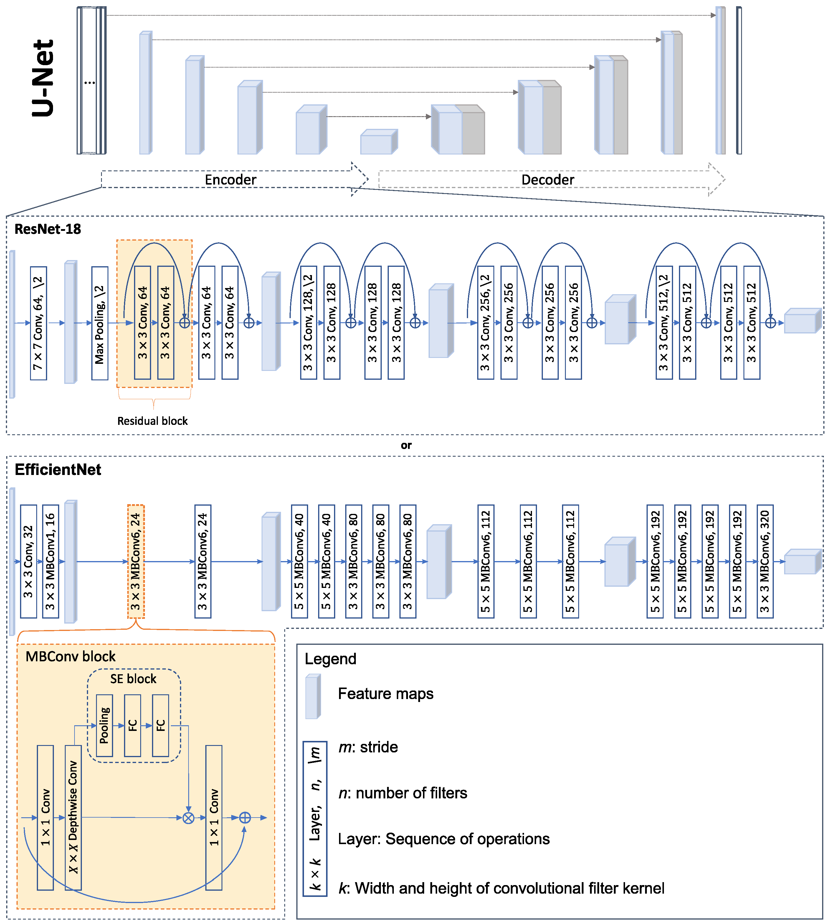
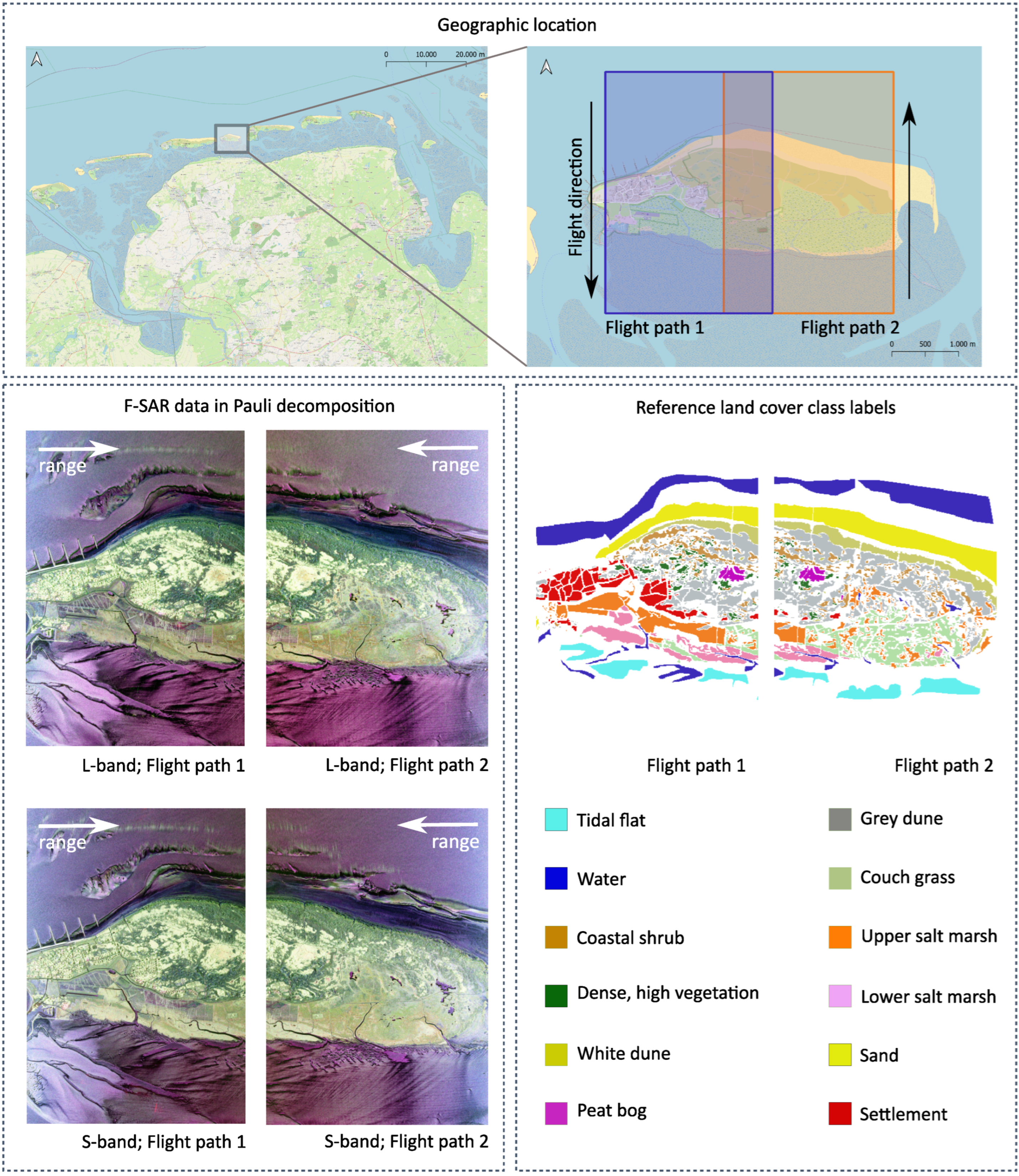
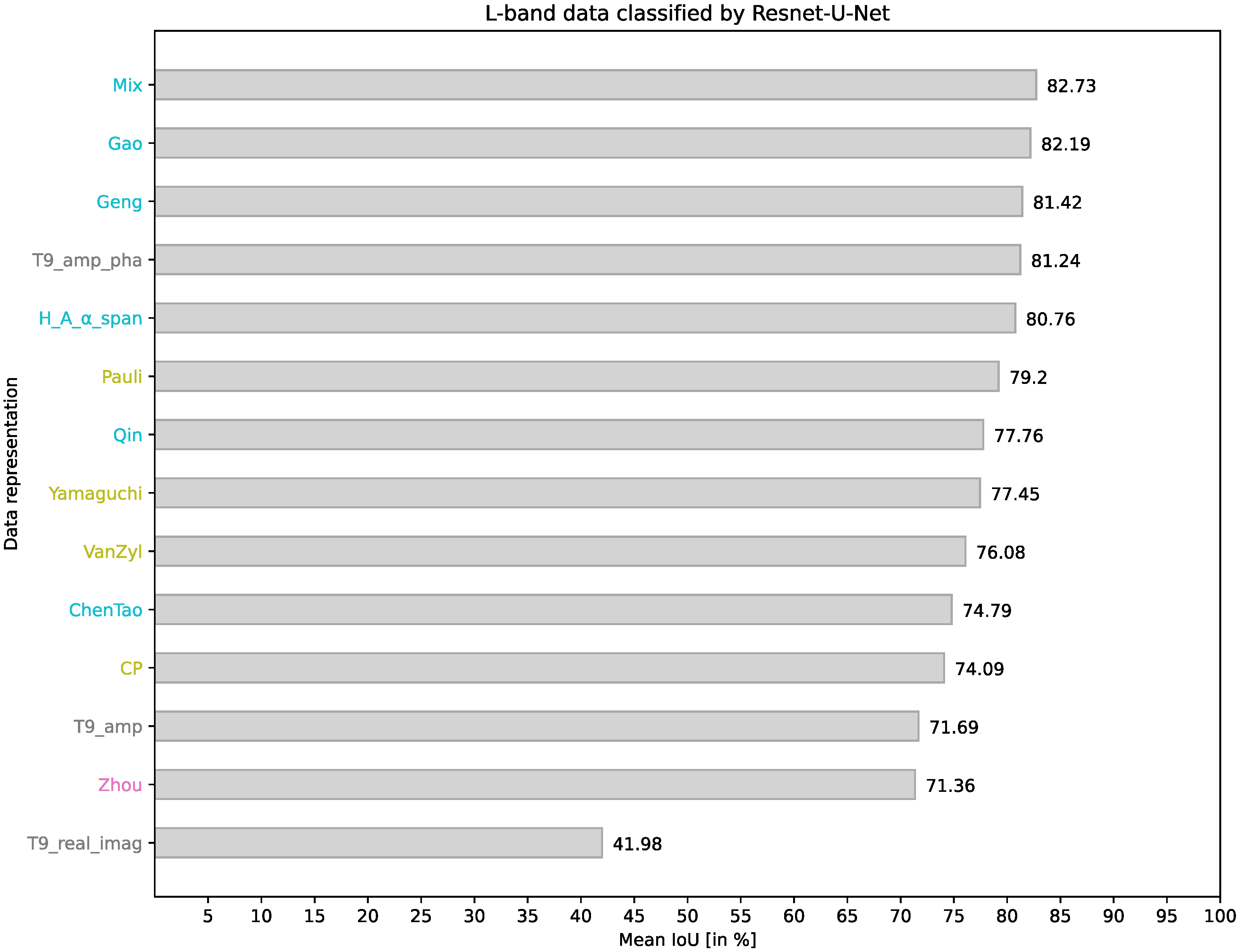
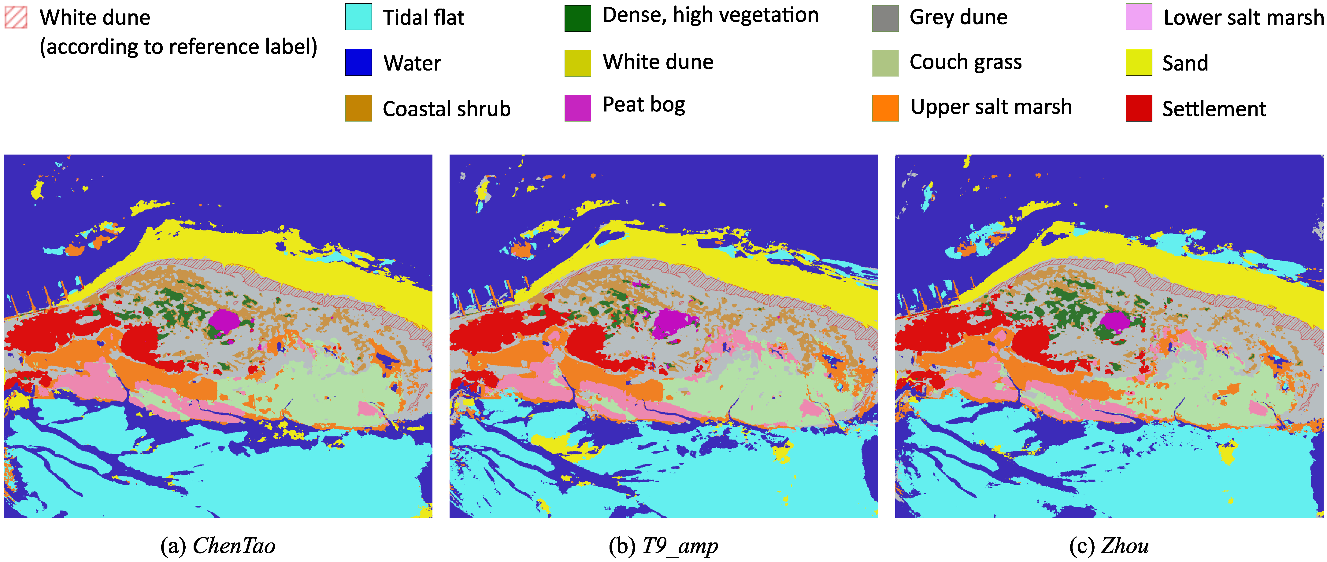
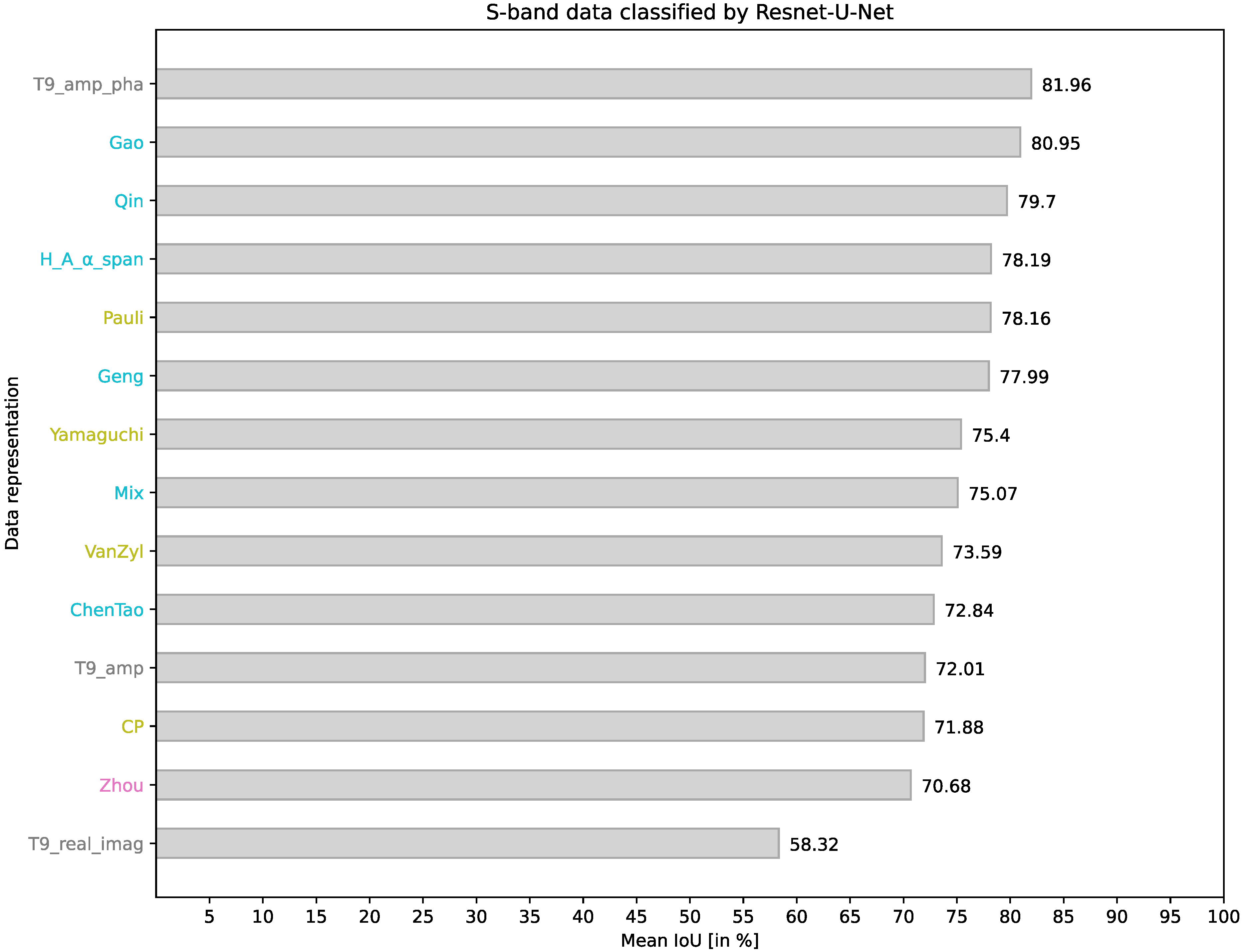
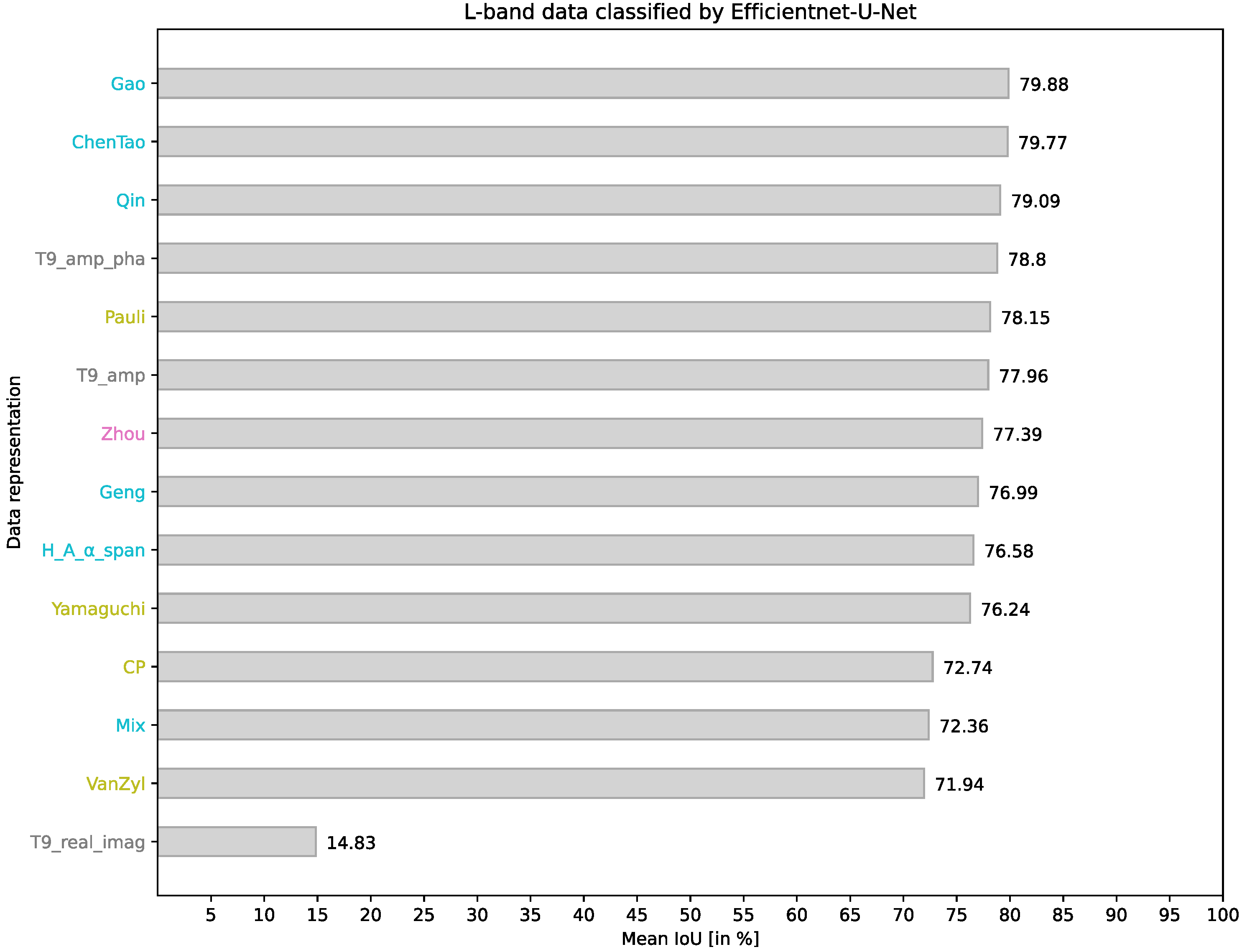
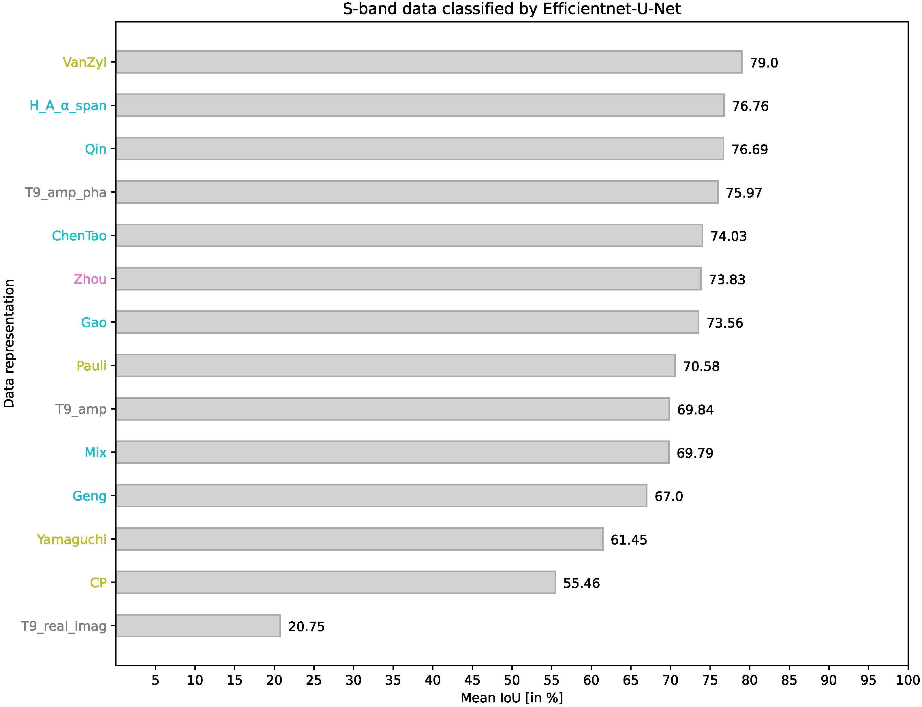
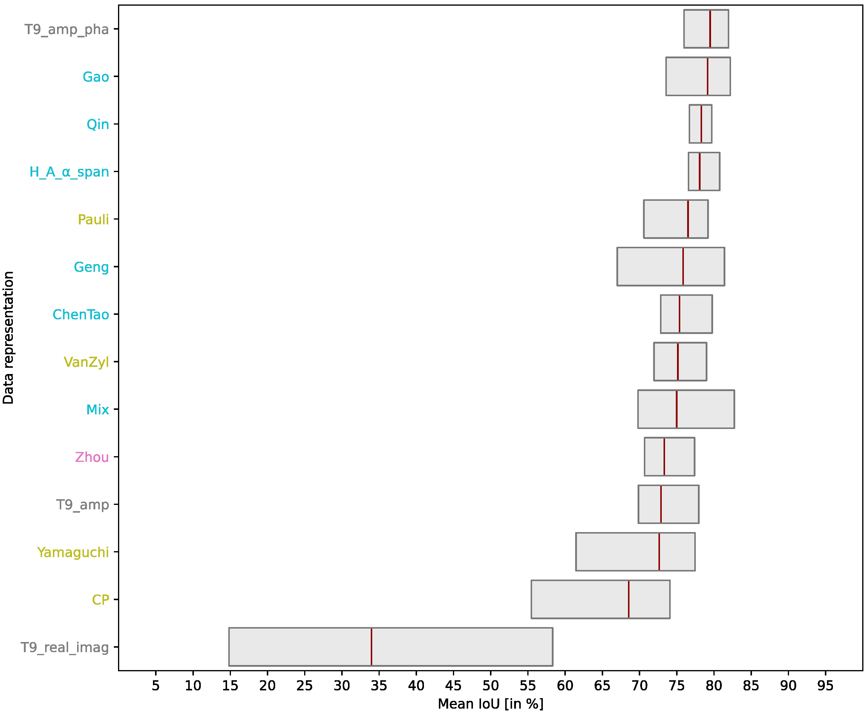
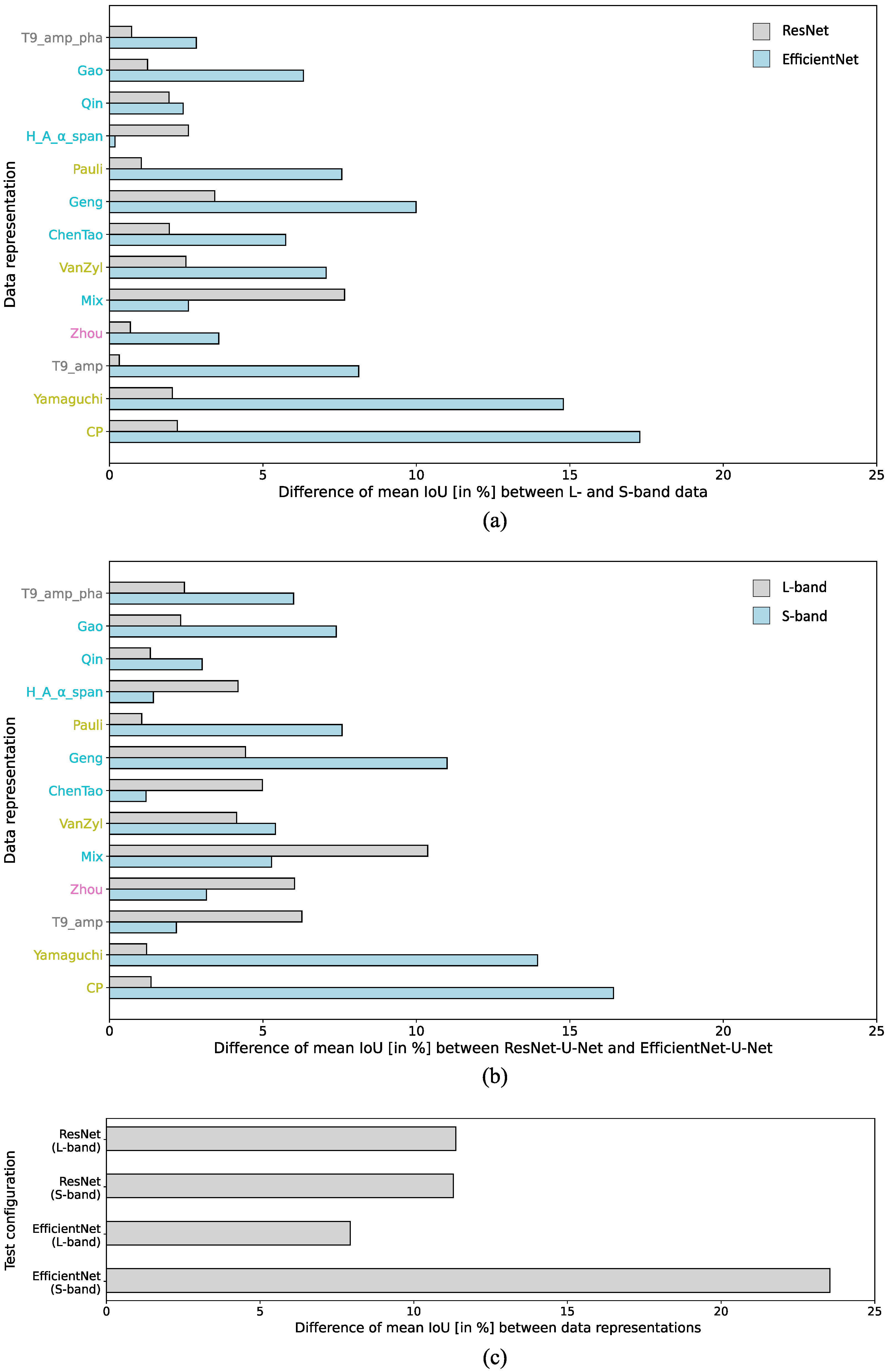
Table 1.
Real-valued PolSAR data representations used as input for CNN-based image segmentation.
| Category | Description | Components | Related Publications |
|---|---|---|---|
| -elements | T9_real_imag | , , , , , , , , | [35,36,37,38,39,40,41,42,43,44,45,46] |
| T9_amp_pha | , , , ||, , ||, , ||, | [47] | |
| T9_amp | , , , ||, ||, || | [58] | |
| -feature vector | Zhou | , , , , , | [20,48,49,50,51,52,53] |
| Target decomposition | Pauli | , , | [31] |
| Yamaguchi | , , | [59] | |
| VanZyl | , , | [60] | |
| CP | H, A, | [54,59] | |
| Combination | Gao | , , , , , , , , | [61] |
| Geng | , , , ||, ||, ||, , , | [62] | |
| ChenTao | H, A, , span, , | [21] | |
| H_A__span | H, A, , span | [63] | |
| Qin | , , , ||, , ||, , ||, , , A, , , , , | [56] | |
| Mix | H, A, , span, , , , , , ||, , ||, , ||, , , , , , , , , | - |
Table 2.
Percentage of labeled pixels per class contained in the training and the test data.
| TF | W | CS | DV | WD | PB | GD | CG | US | LS | S | SE | |
|---|---|---|---|---|---|---|---|---|---|---|---|---|
| Training | 7.09 | 17.98 | 5.29 | 2.04 | 6.72 | 0.87 | 17.78 | 8.17 | 8.01 | 5.85 | 14.92 | 5.28 |
| Test | 8.07 | 17.31 | 3.65 | 1.43 | 6.44 | 1.15 | 19.88 | 7.56 | 9.51 | 4.75 | 14.62 | 5.63 |
Table 3.
Segmentation results for L-band data obtained using ResNet-U-Net measured by class-wise and mean IoU [in %]. The highest scores for each class are printed in bold.
Table 3.
Segmentation results for L-band data obtained using ResNet-U-Net measured by class-wise and mean IoU [in %]. The highest scores for each class are printed in bold.
| Input | TF | W | CS | DV | WD | PB | GD | CG | US | LS | S | SE | Mean |
|---|---|---|---|---|---|---|---|---|---|---|---|---|---|
| T9_real_imag | 13.42 | 78.50 | 56.10 | 36.61 | 7.70 | 79.30 | 38.79 | 20.76 | 1.54 | 29.48 | 49.07 | 92.53 | 41.98 |
| T9_amp_pha | 98.22 | 97.73 | 69.66 | 56.44 | 78.61 | 92.84 | 78.07 | 66.47 | 64.26 | 83.74 | 97.06 | 91.81 | 81.24 |
| T9_amp | 91.87 | 95.49 | 64.89 | 49.91 | 0.00 | 83.83 | 64.60 | 75.33 | 70.25 | 76.41 | 95.68 | 91.99 | 71.69 |
| Pauli | 90.07 | 94.93 | 67.01 | 62.48 | 67.90 | 87.39 | 75.66 | 73.56 | 65.47 | 77.15 | 97.08 | 91.70 | 79.20 |
| Zhou | 96.59 | 95.17 | 57.75 | 46.36 | 0.00 | 91.52 | 64.59 | 75.51 | 61.20 | 79.01 | 97.12 | 91.49 | 71.36 |
| Gao | 97.80 | 95.24 | 70.34 | 58.03 | 82.30 | 87.34 | 79.33 | 77.68 | 63.65 | 84.46 | 98.01 | 92.14 | 82.19 |
| CP | 94.36 | 95.13 | 57.58 | 44.87 | 65.20 | 79.40 | 76.18 | 56.03 | 73.00 | 58.48 | 94.64 | 94.18 | 74.09 |
| Yamaguchi | 93.11 | 96.36 | 66.09 | 52.19 | 74.33 | 86.30 | 75.78 | 68.02 | 58.03 | 72.19 | 99.00 | 87.95 | 77.45 |
| VanZyl | 89.66 | 96.22 | 61.88 | 46.61 | 64.30 | 96.43 | 72.15 | 71.80 | 58.88 | 70.70 | 94.31 | 90.02 | 76.08 |
| ChenTao | 97.55 | 98.50 | 64.43 | 51.62 | 0.00 | 91.91 | 66.78 | 76.42 | 73.67 | 86.53 | 97.74 | 92.29 | 74.79 |
| H_A__span | 92.08 | 97.51 | 67.78 | 59.37 | 69.22 | 92.57 | 77.38 | 74.60 | 70.65 | 76.13 | 98.89 | 92.97 | 80.76 |
| Geng | 94.70 | 96.36 | 70.47 | 54.91 | 80.45 | 85.69 | 77.77 | 75.30 | 66.11 | 83.17 | 97.53 | 94.53 | 81.42 |
| Qin | 92.83 | 92.02 | 60.69 | 44.37 | 78.88 | 83.46 | 78.16 | 73.69 | 67.47 | 84.01 | 92.33 | 85.26 | 77.76 |
| Mix | 90.57 | 96.26 | 67.66 | 63.65 | 76.32 | 95.90 | 78.59 | 72.65 | 70.53 | 88.57 | 98.75 | 93.31 | 82.73 |
Table 4.
Segmentation results of S-band data obtained using ResNet-U-Net measured by class-wise and mean IoU [in %]. The highest scores for each class are printed in bold.
Table 4.
Segmentation results of S-band data obtained using ResNet-U-Net measured by class-wise and mean IoU [in %]. The highest scores for each class are printed in bold.
| Input | TF | W | CS | DV | WD | PB | GD | CG | US | LS | S | SE | Mean |
|---|---|---|---|---|---|---|---|---|---|---|---|---|---|
| T9_real_imag | 72.05 | 86.54 | 57.45 | 27.62 | 2.69 | 72.25 | 52.98 | 41.32 | 45.25 | 61.07 | 91.55 | 89.03 | 58.32 |
| T9_amp_pha | 94.72 | 97.86 | 64.64 | 53.73 | 70.77 | 95.30 | 77.27 | 80.77 | 73.32 | 87.10 | 97.50 | 90.59 | 81.96 |
| T9_amp | 93.19 | 95.81 | 57.84 | 53.53 | 0.00 | 94.35 | 62.56 | 77.30 | 64.25 | 78.69 | 97.27 | 89.39 | 72.01 |
| Pauli | 86.33 | 95.49 | 60.53 | 51.11 | 59.78 | 95.01 | 74.00 | 75.48 | 65.81 | 82.66 | 97.39 | 94.29 | 78.16 |
| Zhou | 77.27 | 90.11 | 62.71 | 40.84 | 0.00 | 91.84 | 66.05 | 77.36 | 72.24 | 82.57 | 95.49 | 91.67 | 70.68 |
| Gao | 92.27 | 95.98 | 68.83 | 60.23 | 69.15 | 88.78 | 75.34 | 76.57 | 67.76 | 87.02 | 96.21 | 93.23 | 80.95 |
| CP | 83.12 | 89.85 | 58.47 | 53.46 | 72.55 | 93.34 | 73.49 | 56.00 | 62.31 | 50.20 | 76.53 | 93.22 | 71.88 |
| Yamaguchi | 78.27 | 93.46 | 61.28 | 40.17 | 66.50 | 92.94 | 73.45 | 68.93 | 61.81 | 84.15 | 93.08 | 90.78 | 75.40 |
| VanZyl | 86.10 | 95.71 | 62.26 | 0.00 | 61.52 | 95.39 | 73.73 | 74.82 | 63.20 | 82.38 | 95.13 | 92.87 | 73.59 |
| ChenTao | 95.16 | 97.00 | 60.31 | 58.23 | 0.00 | 93.75 | 66.12 | 72.57 | 71.48 | 75.43 | 94.44 | 89.63 | 72.84 |
| H_A__span | 96.66 | 96.91 | 63.41 | 52.54 | 61.70 | 92.21 | 70.36 | 73.96 | 57.87 | 85.64 | 95.81 | 91.24 | 78.19 |
| Geng | 95.40 | 96.08 | 66.69 | 46.04 | 67.06 | 88.01 | 73.53 | 77.35 | 55.97 | 82.70 | 96.28 | 90.80 | 77.99 |
| Qin | 97.38 | 97.41 | 61.34 | 49.81 | 52.51 | 97.21 | 74.37 | 80.51 | 69.04 | 88.58 | 96.18 | 92.10 | 79.70 |
| Mix | 98.46 | 97.73 | 64.82 | 51.21 | 0.00 | 94.44 | 66.77 | 76.12 | 71.1 | 89.62 | 96.05 | 94.56 | 75.07 |
Table 5.
Segmentation results of L-band data obtained using EfficientNet-U-Net measured by class-wise and mean IoU [in %]. The highest scores for each class are printed in bold.
Table 5.
Segmentation results of L-band data obtained using EfficientNet-U-Net measured by class-wise and mean IoU [in %]. The highest scores for each class are printed in bold.
| Input | TF | W | CS | DV | WD | PB | GD | CG | US | LS | S | SE | Mean |
|---|---|---|---|---|---|---|---|---|---|---|---|---|---|
| T9_real_imag | 0.00 | 32.32 | 37.58 | 27.43 | 0.00 | 0.00 | 27.34 | 0.00 | 0.00 | 0.00 | 1.22 | 52.00 | 14.83 |
| T9_amp_pha | 96.59 | 96.91 | 64.81 | 49.09 | 74.06 | 80.02 | 77.67 | 68.72 | 68.09 | 81.91 | 95.97 | 91.81 | 78.80 |
| T9_amp | 86.51 | 95.21 | 64.11 | 49.82 | 83.10 | 71.81 | 78.60 | 72.88 | 67.71 | 76.50 | 97.27 | 92.03 | 77.96 |
| Pauli | 82.62 | 92.83 | 66.89 | 61.81 | 75.03 | 91.25 | 75.80 | 67.46 | 62.21 | 73.31 | 94.69 | 93.93 | 78.15 |
| Zhou | 89.13 | 94.73 | 69.45 | 48.77 | 80.18 | 75.49 | 75.84 | 69.08 | 68.40 | 71.91 | 96.06 | 89.67 | 77.39 |
| Gao | 89.62 | 95.08 | 67.22 | 55.90 | 85.86 | 88.43 | 79.41 | 72.05 | 66.58 | 70.17 | 97.89 | 90.32 | 79.88 |
| CP | 90.22 | 91.96 | 53.68 | 47.09 | 75.61 | 81.45 | 69.03 | 55.85 | 65.42 | 58.84 | 90.86 | 92.87 | 72.74 |
| Yamaguchi | 84.64 | 92.48 | 64.41 | 53.88 | 75.25 | 85.07 | 75.93 | 63.56 | 60.80 | 73.02 | 98.50 | 87.34 | 76.24 |
| VanZyl | 93.37 | 93.61 | 53.00 | 36.12 | 68.77 | 71.23 | 72.70 | 67.81 | 55.86 | 67.68 | 92.03 | 91.12 | 71.94 |
| ChenTao | 98.67 | 95.89 | 67.03 | 55.43 | 72.41 | 86.90 | 75.91 | 65.49 | 67.34 | 84.76 | 94.03 | 93.32 | 79.77 |
| H_A__span | 85.42 | 91.73 | 62.94 | 49.29 | 79.01 | 83.05 | 77.99 | 68.71 | 64.04 | 69.33 | 94.60 | 92.82 | 76.58 |
| Geng | 81.70 | 92.82 | 67.64 | 56.80 | 83.05 | 81.04 | 77.28 | 64.39 | 60.87 | 70.83 | 96.65 | 90.75 | 76.99 |
| Qin | 96.37 | 96.16 | 61.77 | 52.49 | 80.90 | 86.53 | 75.58 | 61.88 | 62.78 | 84.23 | 97.45 | 92.94 | 79.09 |
| Mix | 95.27 | 95.62 | 52.79 | 30.20 | 63.70 | 78.31 | 71.90 | 60.36 | 63.12 | 73.68 | 97.04 | 86.34 | 72.36 |
Table 6.
Segmentation results of S-band data obtained using EfficientNet-U-Net measured by class-wise and mean IoU (in %). The highest scores for each class are printed in bold.
Table 6.
Segmentation results of S-band data obtained using EfficientNet-U-Net measured by class-wise and mean IoU (in %). The highest scores for each class are printed in bold.
| Input | TF | W | CS | DV | WD | PB | GD | CG | US | LS | S | SE | Mean |
|---|---|---|---|---|---|---|---|---|---|---|---|---|---|
| T9_real_imag | 0.00 | 0.10 | 41.78 | 20.21 | 0.00 | 55.65 | 20.37 | 7.65 | 1.45 | 38.17 | 0.00 | 63.60 | 20.75 |
| T9_amp_pha | 94.11 | 96.95 | 60.05 | 40.22 | 49.04 | 91.45 | 75.50 | 70.65 | 74.67 | 74.95 | 94.53 | 89.45 | 75.97 |
| T9_amp | 70.89 | 88.26 | 49.66 | 37.47 | 51.37 | 90.10 | 70.96 | 61.03 | 63.02 | 67.20 | 96.55 | 91.53 | 69.84 |
| Pauli | 88.23 | 96.62 | 60.31 | 37.06 | 0.00 | 91.74 | 65.89 | 73.98 | 64.73 | 84.22 | 94.05 | 90.08 | 70.58 |
| Zhou | 86.74 | 92.23 | 54.86 | 36.42 | 65.09 | 84.80 | 71.91 | 72.47 | 63.96 | 74.46 | 92.15 | 90.92 | 73.83 |
| Gao | 83.19 | 93.54 | 63.58 | 36.07 | 53.84 | 77.35 | 70.66 | 68.89 | 66.15 | 80.26 | 96.15 | 93.05 | 73.56 |
| CP | 64.28 | 81.20 | 46.50 | 49.39 | 24.87 | 46.83 | 62.84 | 48.14 | 55.67 | 48.26 | 49.69 | 87.89 | 55.46 |
| Yamaguchi | 41.30 | 70.80 | 55.79 | 41.74 | 36.08 | 74.49 | 65.31 | 61.70 | 55.93 | 76.25 | 72.69 | 85.35 | 61.45 |
| VanZyl | 89.28 | 94.94 | 63.31 | 52.26 | 54.03 | 96.47 | 74.24 | 78.16 | 72.33 | 85.71 | 94.54 | 92.74 | 79.00 |
| ChenTao | 95.62 | 94.83 | 54.58 | 47.37 | 70.48 | 84.70 | 76.67 | 59.77 | 71.99 | 47.83 | 93.72 | 90.83 | 74.03 |
| H_A__span | 93.72 | 96.42 | 64.01 | 40.29 | 63.57 | 93.36 | 71.18 | 70.92 | 59.78 | 83.40 | 94.10 | 90.44 | 76.76 |
| Geng | 79.86 | 92.22 | 58.31 | 31.66 | 33.71 | 68.37 | 61.75 | 68.39 | 54.81 | 73.23 | 91.79 | 89.85 | 67.00 |
| Qin | 84.71 | 93.59 | 59.03 | 50.62 | 64.54 | 75.20 | 78.03 | 74.58 | 75.24 | 76.84 | 93.26 | 94.61 | 76.69 |
| Mix | 95.44 | 93.58 | 39.03 | 33.07 | 59.65 | 78.36 | 69.06 | 59.98 | 65.42 | 66.90 | 90.80 | 86.18 | 69.79 |
Disclaimer/Publisher’s Note: The statements, opinions and data contained in all publications are solely those of the individual author(s) and contributor(s) and not of MDPI and/or the editor(s). MDPI and/or the editor(s) disclaim responsibility for any injury to people or property resulting from any ideas, methods, instructions or products referred to in the content. |
© 2023 by the authors. Licensee MDPI, Basel, Switzerland. This article is an open access article distributed under the terms and conditions of the Creative Commons Attribution (CC BY) license (https://creativecommons.org/licenses/by/4.0/).
Share and Cite
MDPI and ACS Style
Hochstuhl, S.; Pfeffer, N.; Thiele, A.; Hammer, H.; Hinz, S. Your Input Matters—Comparing Real-Valued PolSAR Data Representations for CNN-Based Segmentation. Remote Sens. 2023, 15, 5738. https://doi.org/10.3390/rs15245738
AMA Style
Hochstuhl S, Pfeffer N, Thiele A, Hammer H, Hinz S. Your Input Matters—Comparing Real-Valued PolSAR Data Representations for CNN-Based Segmentation. Remote Sensing. 2023; 15(24):5738. https://doi.org/10.3390/rs15245738
Chicago/Turabian StyleHochstuhl, Sylvia, Niklas Pfeffer, Antje Thiele, Horst Hammer, and Stefan Hinz. 2023. "Your Input Matters—Comparing Real-Valued PolSAR Data Representations for CNN-Based Segmentation" Remote Sensing 15, no. 24: 5738. https://doi.org/10.3390/rs15245738
Note that from the first issue of 2016, this journal uses article numbers instead of page numbers. See further details here.