
Extracting Plastic Greenhouses from Remote Sensing Images with a Novel U-FDS Net


1
School of Information Engineering, Nanchang Hangkong University, Nanchang 330063, China
2
College of Geoscience and Surveying Engineering, China University of Mining & Technology, Beijing 100083, China
*
Author to whom correspondence should be addressed.
Remote Sens. 2023, 15(24), 5736; https://doi.org/10.3390/rs15245736
Submission received: 17 October 2023
/
Revised: 10 December 2023
/
Accepted: 11 December 2023
/
Published: 15 December 2023
(This article belongs to the Special Issue Multisource Remote Sensing Image Interpretation and Application)
Abstract
:The fast and accurate extraction of plastic greenhouses over large areas is important for environmental and agricultural management. Traditional spectral index methods and object-based methods can suffer from poor transferability or high computational costs. Current deep learning-based algorithms are seldom specifically aimed at extracting plastic greenhouses at large scales. To extract plastic greenhouses at large scales with high accuracy, this study proposed a new deep learning-based network, U-FDS Net, specifically for plastic greenhouse extraction over large areas. U-FDS Net combines full-scale dense connections and adaptive deep supervision and has strong future fusion capabilities, allowing more accurate extraction results. To test the extraction accuracy, this study compiled new greenhouse datasets covering Beijing and Shandong with a total number of more than 12,000 image samples. The results showed that the proposed U-FDS net is particularly suitable for complex backgrounds and reducing false positive conditions for nongreenhouse ground objects, with the highest mIoU (mean intersection over union) an increase of ~2%. This study provides a high-performance method for plastic greenhouse extraction to enable environmental management, pollution control and agricultural plans.
1. Introduction
The rapid increase in global population has increased the demand for producing food, vegetables and fruits on limited arable land [1,2]. Furthermore, this arable land is gradually being threatened by urbanization and climate change [3]. Therefore, traditional production and planting methods cannot meet the demands of rapidly developing societies [4], and a new type of agriculture facility (plastic greenhouses) is being widely used. These so-called new agricultural facilities mainly refer to plastic greenhouses, which are not limited by season. Through the artificial creation of microenvironments to grow food crops [5] greenhouses can be used to increase agricultural production in complex terrain environments, which greatly improves the utilization of agricultural resources. The popularization of plastic greenhouses has promoted the development of agriculture worldwide and is an important part of agricultural production [6]. However, while creating societal well-being, greenhouses also introduce negative ecological and environmental problems [7,8], such as water pollution, soil acidification and salinization, and biodiversity degradation [9,10,11,12]. Therefore, quickly and accurately extracting the distribution, coverage area and other information of plastic greenhouses is important for environmental management and agricultural planning.
Several previous studies have proposed extracting plastic greenhouses by constructing novel spectral indices [13,14,15] or object-based classification methods [16,17,18]. For example, Yang, et al. [8] proposed a new greenhouse spectral index, RPGI, based on medium spatial resolution remote sensing images. Zhang, et al. [19] proposed an advanced plastic greenhouse spectral index (APGI) based on Sentinel-2 images to map the distribution of large-scale greenhouses. Other studies used object classification-based methods to extract greenhouses. Wu, et al. [20] proposed a practical suburban greenhouse extraction algorithm with Landsat-8 images and an object-based method, suggesting that the object-based method could significantly improve accuracy. However, both methods have some limitations. Specifically, the spectral index method is based on the premise that all greenhouses have the same spectral characteristics, ignoring the “same objects with different spectrum” properties between greenhouses and the “different objects with same spectrum” properties between greenhouses and background objects. Therefore, the spectral index method is very sensitive to noise and easily causes missed classifications and incorrect classifications in practical applications. With changes in the phenological period and roof covering material, such methods may be ineffective. While object-based methods rely on the selection of segmentation parameters and require certain professional experience and prior knowledge. At the same time, the ability to simultaneously extract features is limited, and generalization is poor in complex scenes. Such methods consume considerable computer memory, cannot process large-scale images in parallel and consume considerable time, which is especially prominent in large-range applications [21].
In recent years, with the development of artificial intelligence, deep learning has been widely used in various fields of remote sensing and has achieved superior performance compared with traditional methods in tasks such as fire detection [22], building segmentation [23], hyperspectral image classification [24,25] and other tasks [26,27]. Digital image processing tasks are gradually changing from traditional machine learning algorithms such as support vector machines [28] and random forests [29] to more advanced deep learning algorithms such as deep forests [30]. Convolutional neural networks (CNNs) are the most popular deep learning algorithms in the field of remote sensing [25,31]. Advanced CNNs, such as fully convolutional neural networks [32], U-Net [33] and DeepLab [34], are widely used in remote sensing image segmentation tasks. The development of deep learning methods in recent years has provided an opportunity to employ CNNs to quickly and accurately extract greenhouses [35,36]. Li, et al. [37] compared the performance of three CNN algorithms (YOLO v3, Faster R-CNN and SSD) in greenhouse detection, showing that YOLO v3 achieves the best results. Ma, et al. [38] proposed a dual-task detection framework for greenhouses using ResNet-50 as the feature extraction backbone and compared it with U-Net, achieving a gain of 0.347% in mIoU. Chen, et al. [39] used the U-Net network to extract greenhouses based on Google Earth remote sensing images and obtained an accurate result. Among them, U-Net has achieved success in many remote sensing image analysis tasks because of its advantages of fast calculation and high accuracy [40].
Although Chen, et al. [39] demonstrated the feasibility of U-Net in plastic greenhouse extraction, their study only used a simple transfer of the U-Net network and did not improve its structure. It is worth noting that U-Net was originally proposed as a medical image segmentation network, which is obviously different from the remote sensing of plastic greenhouse images with complex and diverse background features. U-Net++ and U-Net+++ redesigned the skip connection structure of U-Net to improve the extraction results [41,42]. However, U-Net++ cannot explore information at full scale, while U-Net+++ quickly forwards the high-resolution feature maps from the encoder to the decoder, resulting in the direct fusion of feature maps with large differences at the semantic level. Therefore, a network suitable for plastic greenhouse extraction needs a richer receptive field, which can fully capture the semantic features of the objects to be extracted at full scale. This study proposed a new full-scale densely connected adaptive deep supervision network (U-FDS Net) specifically for plastic greenhouse extraction with high-resolution remote sensing imaging over large areas.
The basic assumption of U-FDS Net is that exquisite semantic signals are progressively diluted by full-scale dense hopping connections that reduce the difference between encoders and decoders so that the network can learn semantic features from different granularity feature maps in a more delicate manner. Different information can be learned from feature maps of different scales and granularities, and rich spatial features can be explored through shallow feature maps to capture the boundary information of greenhouses and then distinguish them from roads with similar color and shape features in the background. The advanced texture details of the ground objects are learned through the deep feature map, and buildings similar in shape to a greenhouse can be distinguished. Each small nested structure is followed by an adaptive deep supervision structure and concatenated loss function at the end, which is helpful for the adaptive weighted fusion of branches with feature maps of different scales and degrees of dilution to improve the segmentation accuracy. Moreover, the shallow layers of the network can be trained more fully, and the convergence speed of the model can be improved.
This study proposed a novel plastic greenhouse segmentation model, U-FDS Net, with full-scale dense connections and an adaptive deep supervision structure, which can better integrate global overall information and local detailed information, thereby improving segmentation accuracy. We tested the proposed new model on two self-annotated greenhouse datasets from different regions and at different scales. The results showed that the U-FDS Net proposed in this study achieves the highest performance. Specifically, compared to U-Net, U-Net++, U-Net+++, and Attention U-Net, the proposed method achieves maximum accuracy improvements of ~1.6% and ~1.9% on the two datasets, respectively. The structure of this paper is as follows: Section 2 presents our methods and details of the self-annotated greenhouse dataset used for testing; Section 3 presents the experimental results; Section 4 discusses our methods; and Section 5 presents the conclusions.
2. Materials and Methods
2.1. Network Structure
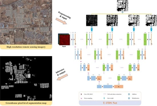
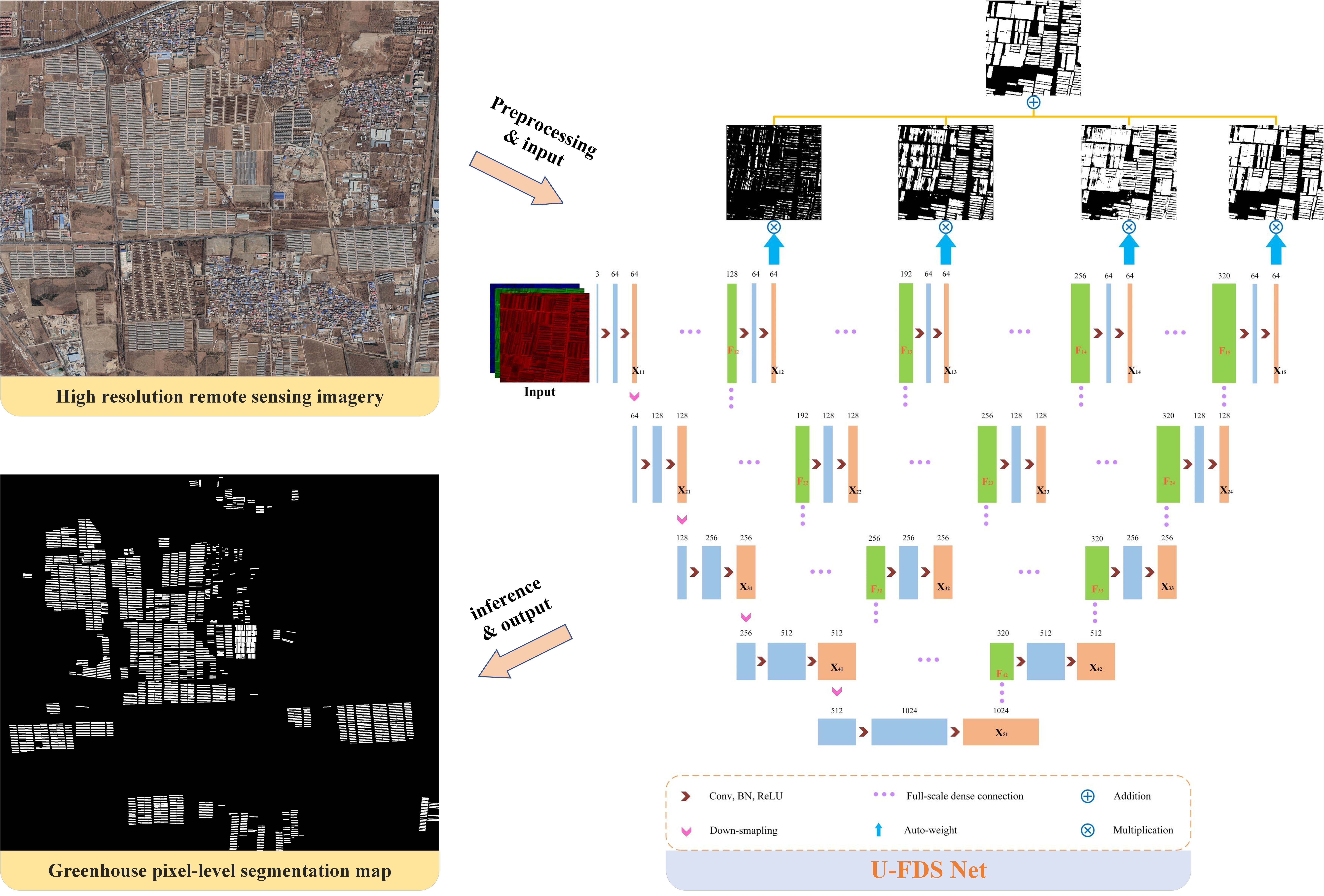
Figure 1 shows the overall structure of the U-FDS Net proposed in this study. On the whole, it is a multi-nested encoder–decoder structure, and different nested structures are closely connected by full-scale dense connections. Each small nested structure is accompanied by a sequential increase in the number of downsampling and upsampling operations and the gradual expansion of the receptive field to hierarchically learn different levels of feature maps. Finally, it is an adaptive deep-supervised feature extraction structure concatenated with a binary cross-entropy loss function after a weighted fusion of the deep supervision results. Small nested structures can provide more accurate global positioning results, while deeply nested structures can offer a precise basis for detail segmentation. With the change in scale and the gradual dilution of the characteristic signal, the network selects the feature maps that are easier to learn in a series of feature maps with different scales and different granularities, and, finally, adaptive weighted fitting is performed to achieve model pruning and improve segmentation accuracy.
2.1.1. Full-Scale Dense Connection
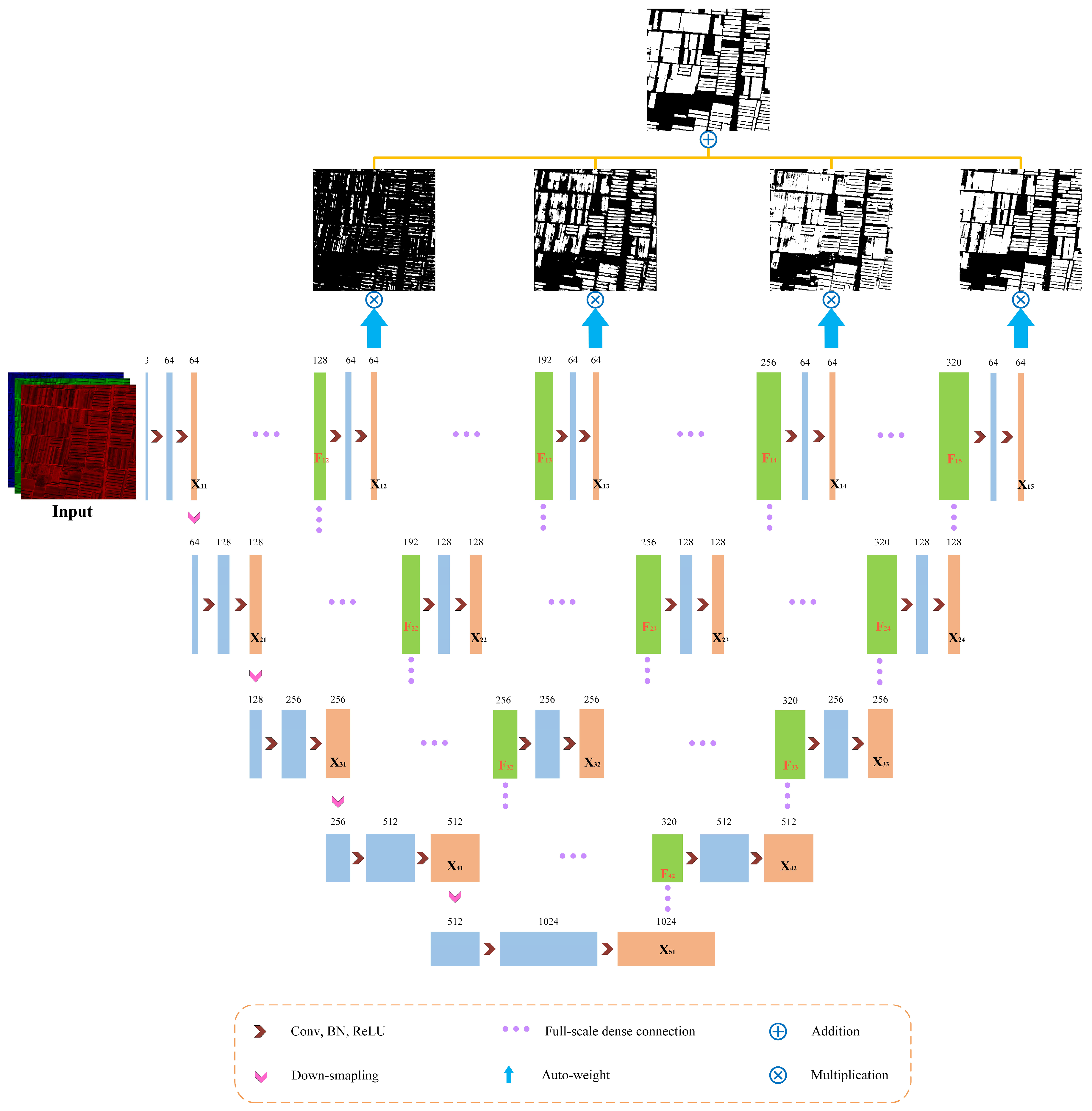
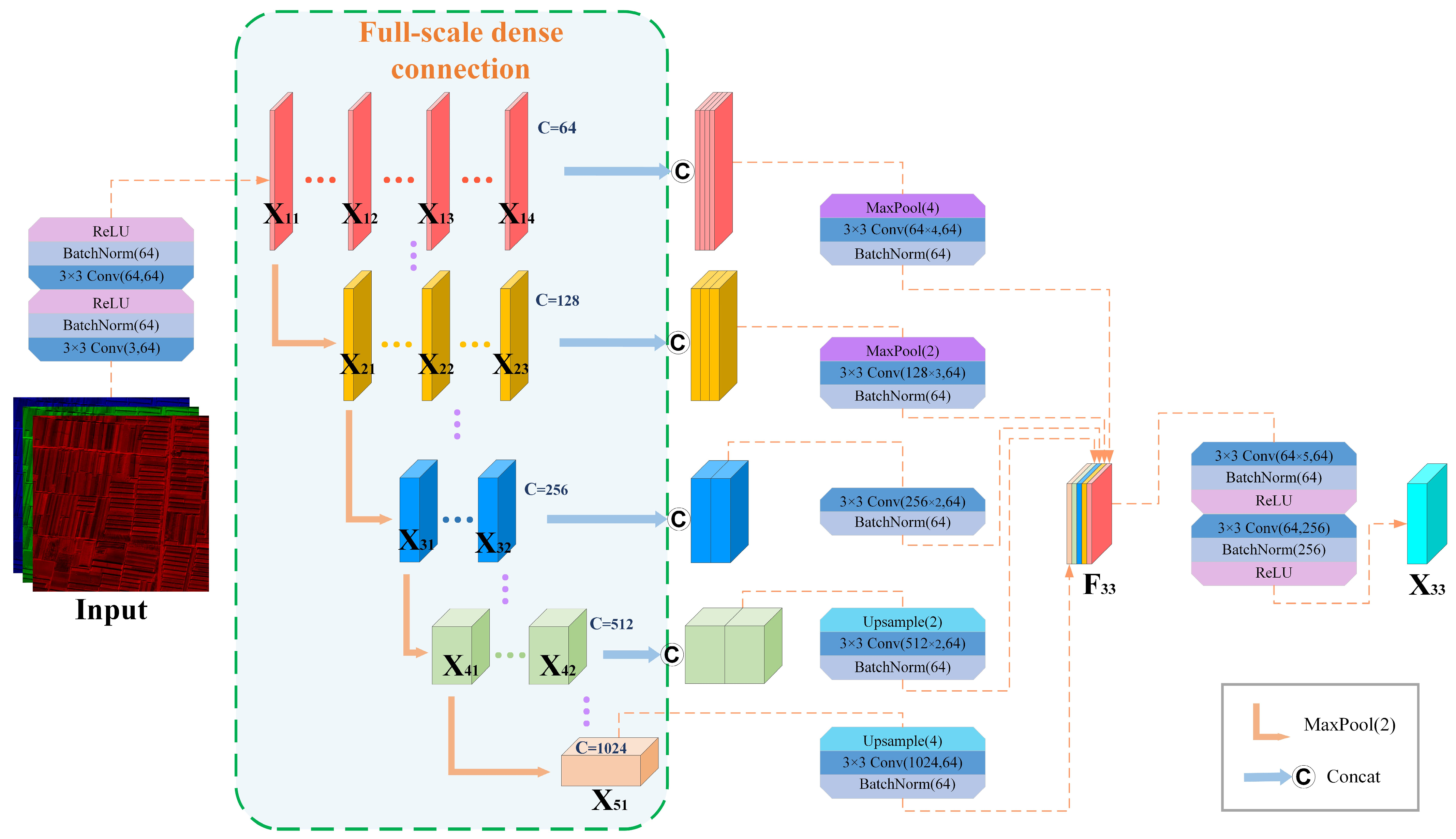
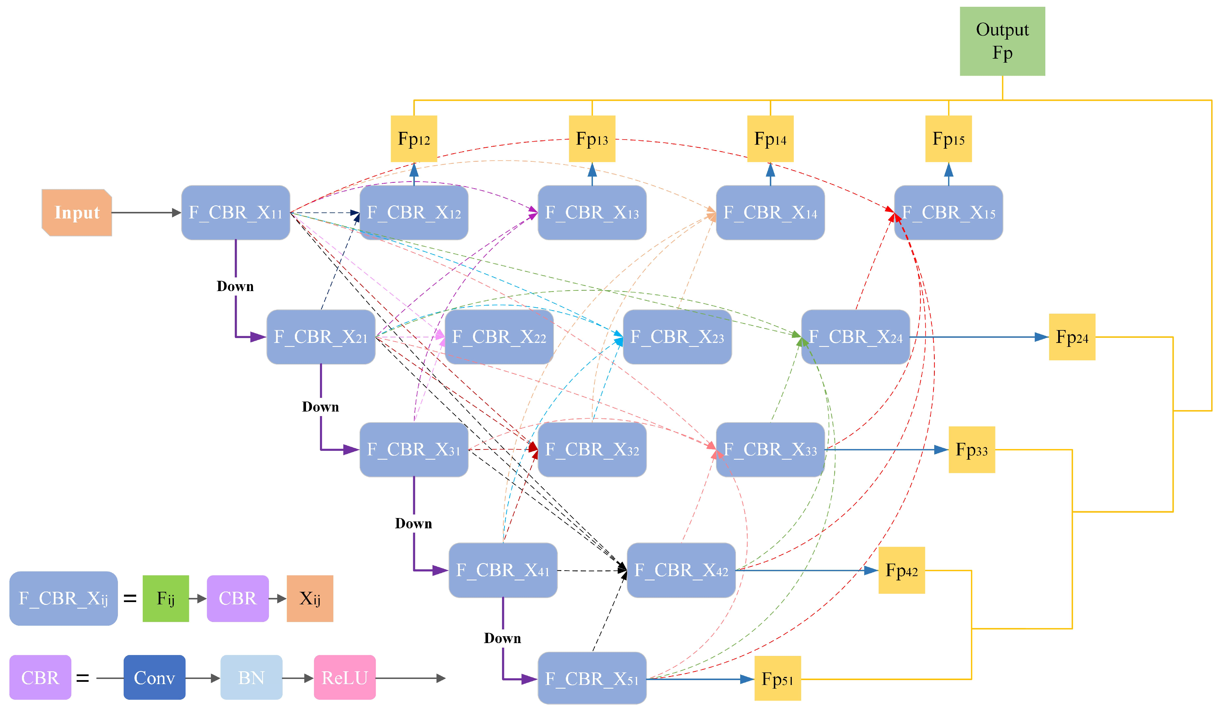
Full-scale dense connections proposed in U-FDS Net can narrow the large-span semantic gap between the encoder and decoder, improve their connectivity, help restore fine-grained details of the target object, and fully explore features at different scales and different degrees of dilution. To ensure maximum information flow between layers in the network, we interconnect the gradually abstracted feature maps to strengthen the interaction between multilevel semantic information. To maintain the feed-forward nature of information, we make each layer of the network obtain input from the previous layers of different scales, perform channel integration and feature fusion on all the obtained information, and then take their own feature information as output to the subsequent layer. Figure 2 shows the detailed full-scale densely connected structure, taking the cascaded result F33 and feature map X33 in row 3, column 3 as an example.
U-FDS Net first unifies the input original image into a feature map X11 with 64 channels through two convolution operations, followed by downsampling based on max pooling, each time reducing the resolution by half (will not lead to information loss). Through downsampling, the coding results in the first column that is closest to the semantic level of the original image are obtained, and then all the feedforward feature maps that provide input to F33 are sequentially obtained. We perform channel concatenation (concat) on the feature maps of different granularity levels in each row to obtain channel integration results of different scales and then perform different levels of scaling operations on the feature streams that are different from the scales of the feature maps to be fused. The downsampling operation used here is max pooling. The unified scale feature map stacks from different scales and different granularities are obtained by up- and downsampling. To filter out redundant information and control the size of the model, we perform a convolution on each of these feature maps to unify the number of channels and connect BatchNorm (BN) after the convolution layer to avoid the vanishing gradient problem in the process of deep network training and accelerate the convergence speed. Next, U-FDS Net aggregates the processed results to obtain the concatenated result F33 and then performs feature extraction and channel unification through two convolution operations to obtain the final result X33 in the third row and third column. To express the nonlinear relationship between input and output in different feature maps, we connect the BN layer of each of two continuous convolution operations in U-FDS Net with the nonsaturating activation function ReLU ().
To better represent the feedforward input source of each decoding feature layer in the full-scale dense connections and the detailed network structure of U-FDS Net, all the feature map stacks represented by Xi,j can be calculated as
where represents the input original data, represents the feature aggregation mechanism implemented by convolution, BN, and ReLU operations, represents a convolution and BN operation, and represent up- and downsampling, respectively, and represents concatenation. According to the formula, each new result to be decoded accepts Xi,j at all previous locations as its input data source to achieve multiscale and multi-granular feature reuse.
2.1.2. Adaptive Deep Supervision Block
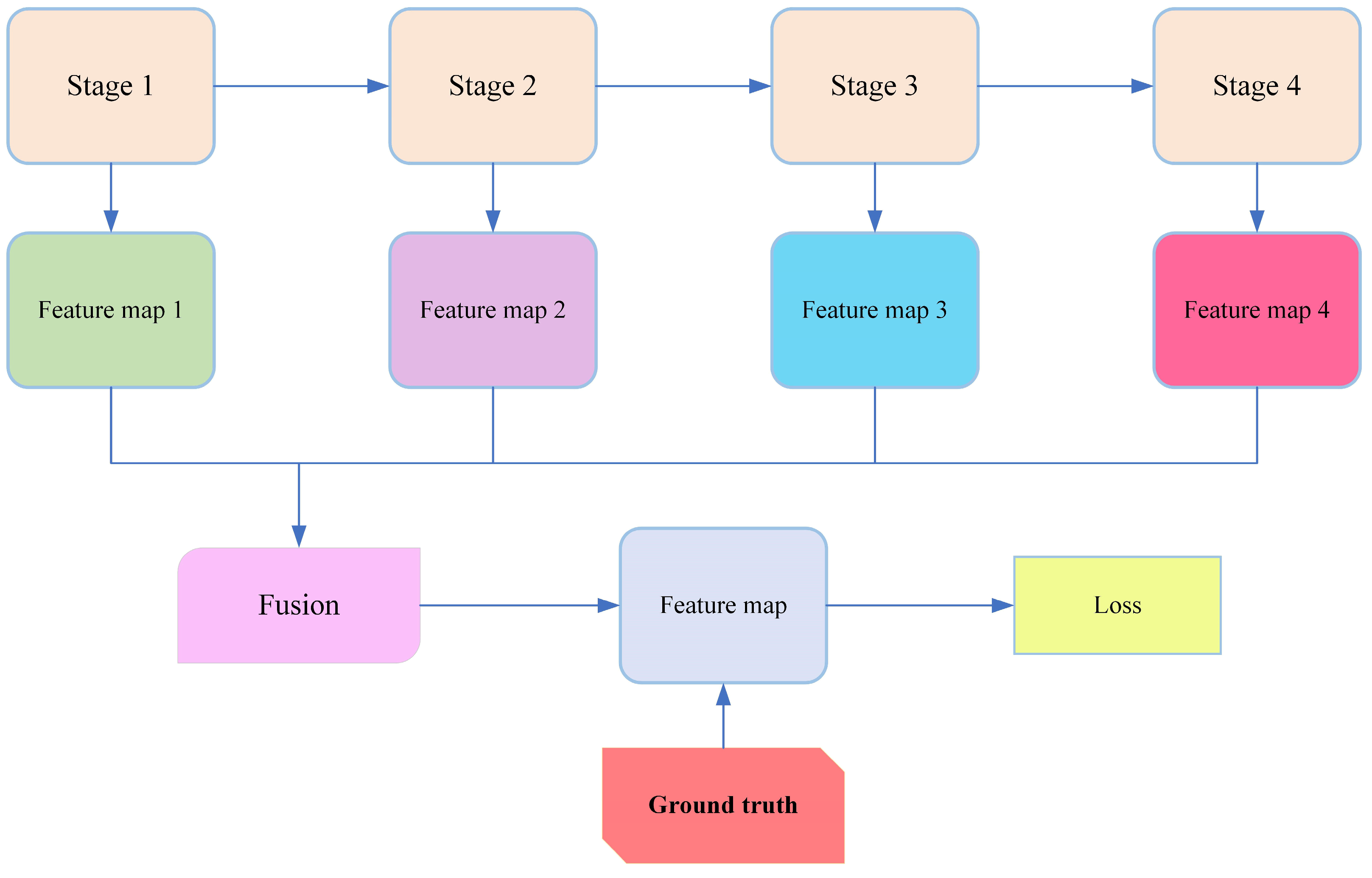
To more reasonably fuse the features captured by the network, an adaptive deep supervision structure is used at the end of each nested structure. All feature maps are fused before outputting, as shown in Figure 3. For the fusion methods of the results of each branch, we propose the idea of making the network learn the weights of each branch by itself for different data because, for data samples with different feature distributions, the proportions of different depth branches in the final result are often different.
Adaptive deep supervision in U-FDS Net is similar to a branch-oriented implicit soft-attention deep supervision mechanism. We add a differentiable coefficient in front of the deep supervised feature map, which can be adjusted automatically according to the gradient backhaul so that the network can assign its own attention to each branch during training. Within each nested structure is an end-to-end classification problem, while each nested structure is more like a regression problem. During training, the network gradually adjusts the weights assigned to each classifier through multiple iterations and finally fits the best representation relationship between each deep supervision result and the ground truth.
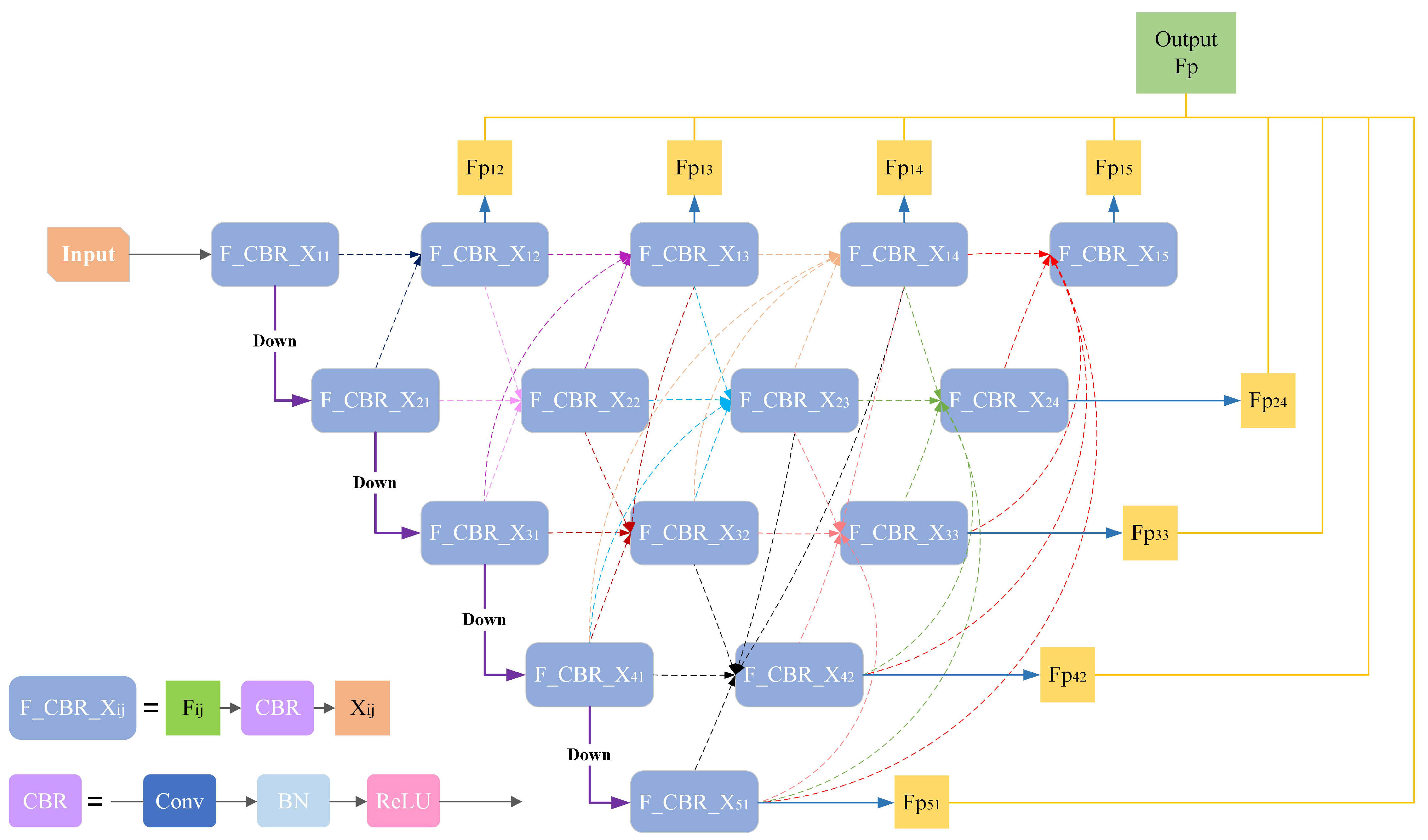
In addition, we provide two other deep supervision schemes for U-FDS Net to change the backhaul gradient flow of the deep network; that is, an adaptive deep-supervised auxiliary classifier is also added to the right branch of U-FDS Net. The step-by-step upsampling scheme (Figure 4) can reduce the image distortion problem caused by the direct upsampling of the underlying ultrasmall resolution feature map to high resolution, while the far-hop upsampling scheme (Figure 5) can lead to faster gradient backhaul.
2.1.3. Lightweight Full-Scale Feature Aggregation Networks
Based on U-FDS Net, we design other lightweight networks with fewer parameters for ablation experiments. It is worth noting that the depth of each network is controlled by the number of CBR structures, which are all set to 2 in this experiment.
Narrow-U-FDS Net: This has the exact same structure as U-FDS Net and greatly reduces the network width on this basis.
En-U-FDS Net: A network structure that gradually expands the difference between the decoder and the encoder (Figure 4), which cancels the dense connection on the basis of U-FDS Net. This structure tends to reuse the features close to the encoder many times, and the features from the encoder will not be quickly forwarded directly to the decoder but will slowly enlarge the difference with the input source with increasing network depth.
De-U-FDS Net: A network structure that gradually progresses the difference between the encoder and the decoder (Figure 5), similar to En-U-FDS Net, also without dense connections. The difference is that this structure tends to use the features on the decoder side, and as the network depth deepens, the features of the encoder are progressively advanced to the decoder multiple times.
The formula expressions of En-U-FDS Net and De-U-FDS Net are shown in Equations (2) and (3), respectively:
En-U-FDS Net:
De-U-FDS Net:
2.2. Self-Annotated Dataset of Plastic Greenhouses
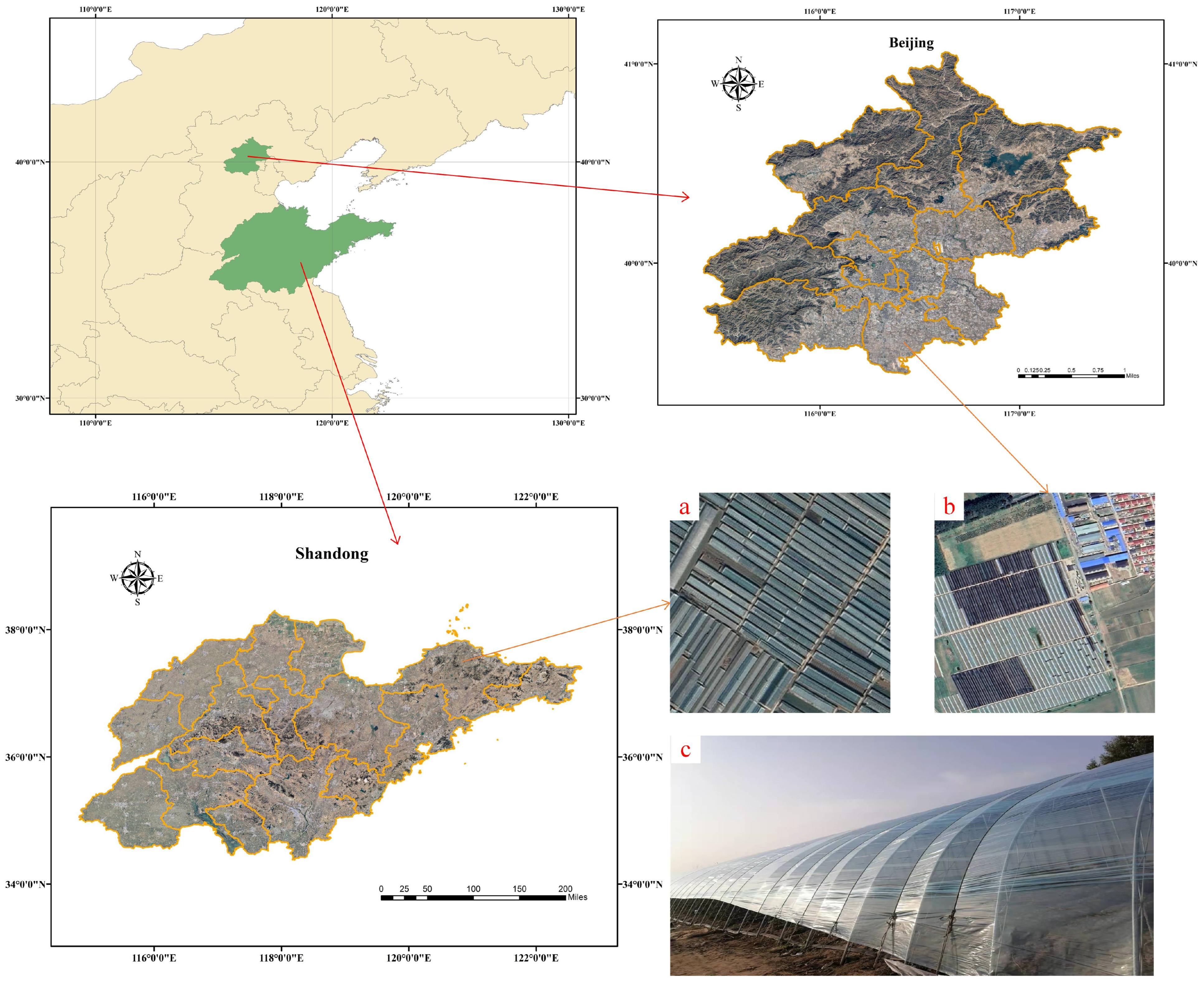
In this study, plastic greenhouse image data from Google Earth remote sensing images with a spatial resolution of 0.95 m for Shandong Province and Beijing are annotated and used. The obtained satellite data is a 24-bit image based on the red (R), green (G), and blue (B) 3 bands. It has features of high resolution and can be directly downloaded and used through various open-source methods without requiring any preprocessing. Shandong Province is located at 114°19′E–122°43′E, 34°22′N–38°23′N, with a total area of 157,800 km2, and is an important vegetable supply base in China. The experimental data were randomly selected from various cities in Shandong Province, cropped into small-sized image blocks of 512 × 512 after annotation, and randomly divided into a training set, validation set, and test set at a ratio of 8:1:1. Beijing is located at 115°25′E–117°30′E and 39°26′N–41°03′N, with a total area of 16,400 km2, and is the capital of China. This dataset consists of 256 × 256 small-sized image patches in Beijing, and the dataset is also divided at a ratio of 8:1:1. This process can be quickly implemented through Python programming. Upon testing, the entire process was completed on a desktop computer (Intel(R) Core(TM) i7-10750H CPU @ 2.60 GHz, 2933 MHz ddr4 Random Access Memory, and Solid State Drives) in approximately 8 min. Table 1 gives detailed information on the self-annotated plastic greenhouse datasets of the two study areas, and Figure 6 shows a schematic diagram of the study area.
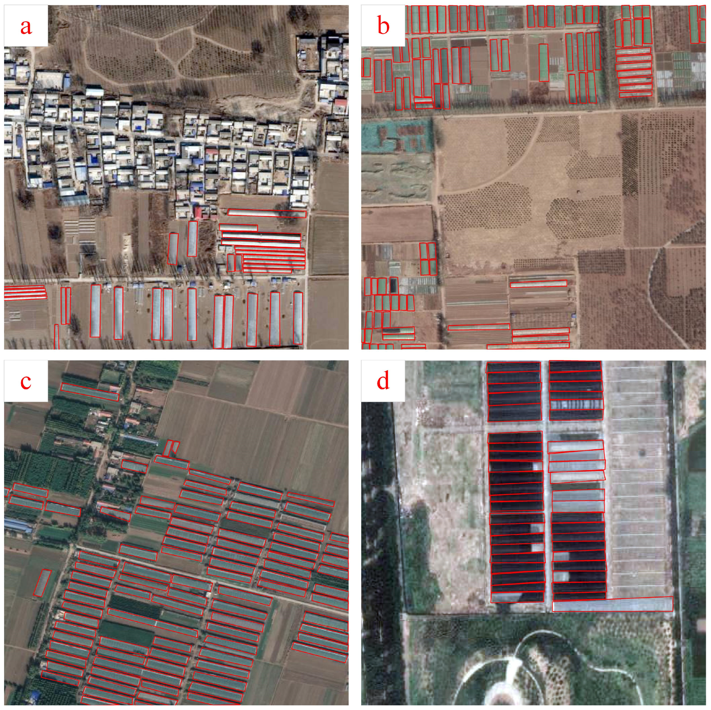
To make plastic greenhouse labels as accurate as possible, by analyzing their distribution and shape, it is found that there are mainly four types of plastic greenhouses in the study area, as shown in Figure 7.
2.3. Experiments
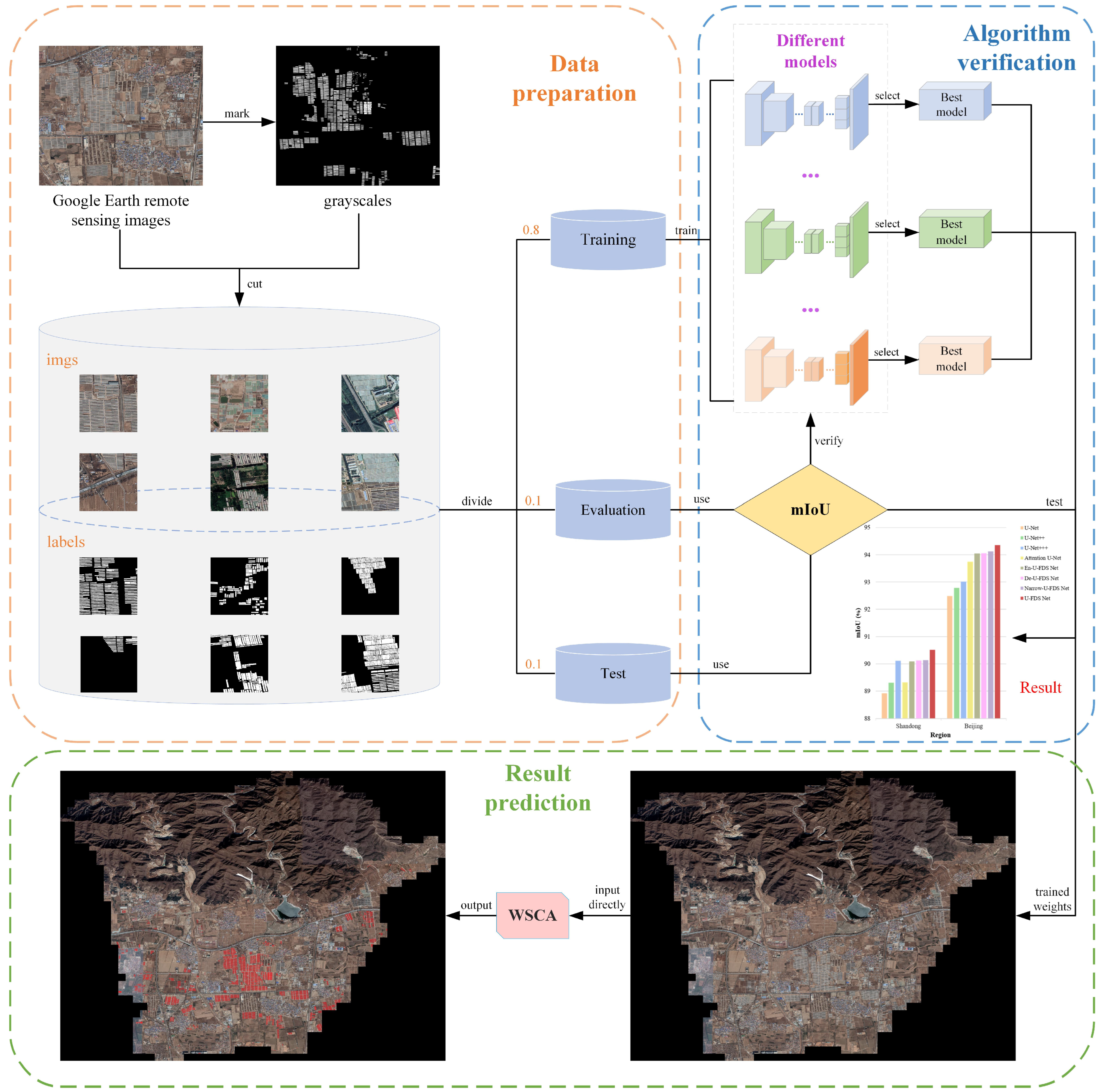
Figure 8 shows the main technical process of extracting plastic greenhouses with three parts: data preparation, algorithm verification and result prediction. In the data preparation part, the downloaded high-resolution remote sensing images were manually annotated by visual interpretation, and the labels were stored in the form of binary grayscale images and were cropped and divided into datasets, as described in Section 2.2. In the algorithm verification part, we use the mean intersection over union (mIoU: %) as the evaluation index to measure the accuracy of each model, filter out the best accuracy weight file of each model according to the verification set, and conduct the accuracy evaluation on the test set. The calculation formula of the mIoU depends on the two-class confusion matrix, and its calculation formula is shown in Equation (4). The specific expression form of the confusion matrix is shown in Table 2. In the result prediction part, we input the original image and the trained weight file into a sliding window segmentation and geographic coordinates add (WSCA) module to complete the prediction of the result.
The equipment hardware of this experiment is an NVIDIA Tesla V100-SXM2 graphics processing unit (GPU) with 32 GB video random access memory (VRAM), and the stream processing unit reaches 5120. The O1-level Apex automatic mixed precision training is used, the optimizer is Adam, the learning rate decay method is cosine annealing, and the batch size of each model is set to the maximum integer multiple of 2 allowed by the VRAM.
The meanings of TP, FN, FP, and TN in the binary confusion matrix used in this experiment are as follows:
- TP: true positive, i.e., the real category of a sample is greenhouse, and the model prediction result is also greenhouse;
- FN: false negative, i.e., the real category of a sample is greenhouse, but the model prediction result is background;
- FP: false positive, i.e., the real category of a sample is background, but the model prediction result is greenhouse;
- TN: true negative, i.e., the real class of a sample is background, and the model prediction result is background.
3. Results and Analysis
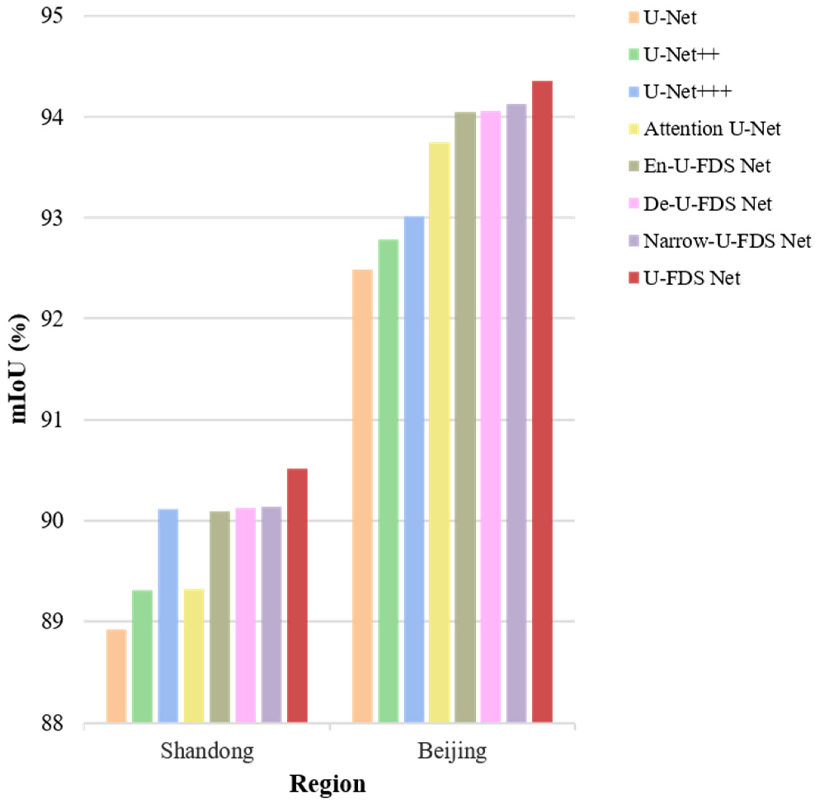
In this study, four typical and widely used networks (U-Net, U-Net++, U-Net+++, and Attention U-Net) were selected as the control group to compare with the En-U-FDS Net, De-U-FDS Net, Narrow-U-FDS Net and U-FDS Net proposed in this study. Table 3 shows the number of parameters and segmentation accuracy of different models in the two greenhouse self-annotated datasets, in which the blue font is the result with the highest accuracy in the control group; the red font is the highest accuracy result in each dataset; and the purple font is the accuracy result of Narrow-U-FDS Net with only a very small number of parameters. A histogram of each accuracy result is shown in Figure 9.
According to Table 3 and Figure 9, we can see that the proposed U-FDS Net achieved the highest segmentation accuracy for both datasets. For the large-scale Shandong dataset, our U-FDS Net achieves performance gains of approximately 1.6% and 0.4% compared to the traditional U-Net and the highest-accuracy U-Net+++ in the control group, respectively. For the small-scale Beijing dataset, U-FDS Net achieves a performance gain of approximately 1.9% and 0.6% compared to the traditional U-Net and the most accurate attention U-Net in the control group, respectively.
Based on the U-FDS Net architecture, the narrow U-FDS Net, which has greatly reduced the network width, has a significant lightweight advantage compared to other models in terms of the number of parameters, and the segmentation accuracy has also been improved. The number of parameters of our reduced network model is only 10.67 M, which is less than that of U-Net. At the same time, it brings approximately 1.2% and 1.6% accuracy improvement over U-Net on the two datasets, respectively, which indicates that the performance gain brought by our architecture comes from the improvement of the architecture, not just due to the increase in the number of parameters. A larger number of parameters further improves segmentation accuracy but at the cost of a significant increase in the required GPU VRAM. U-FDS Net can easily control the model size by changing its width and depth to be mounted on consumer GPUs.
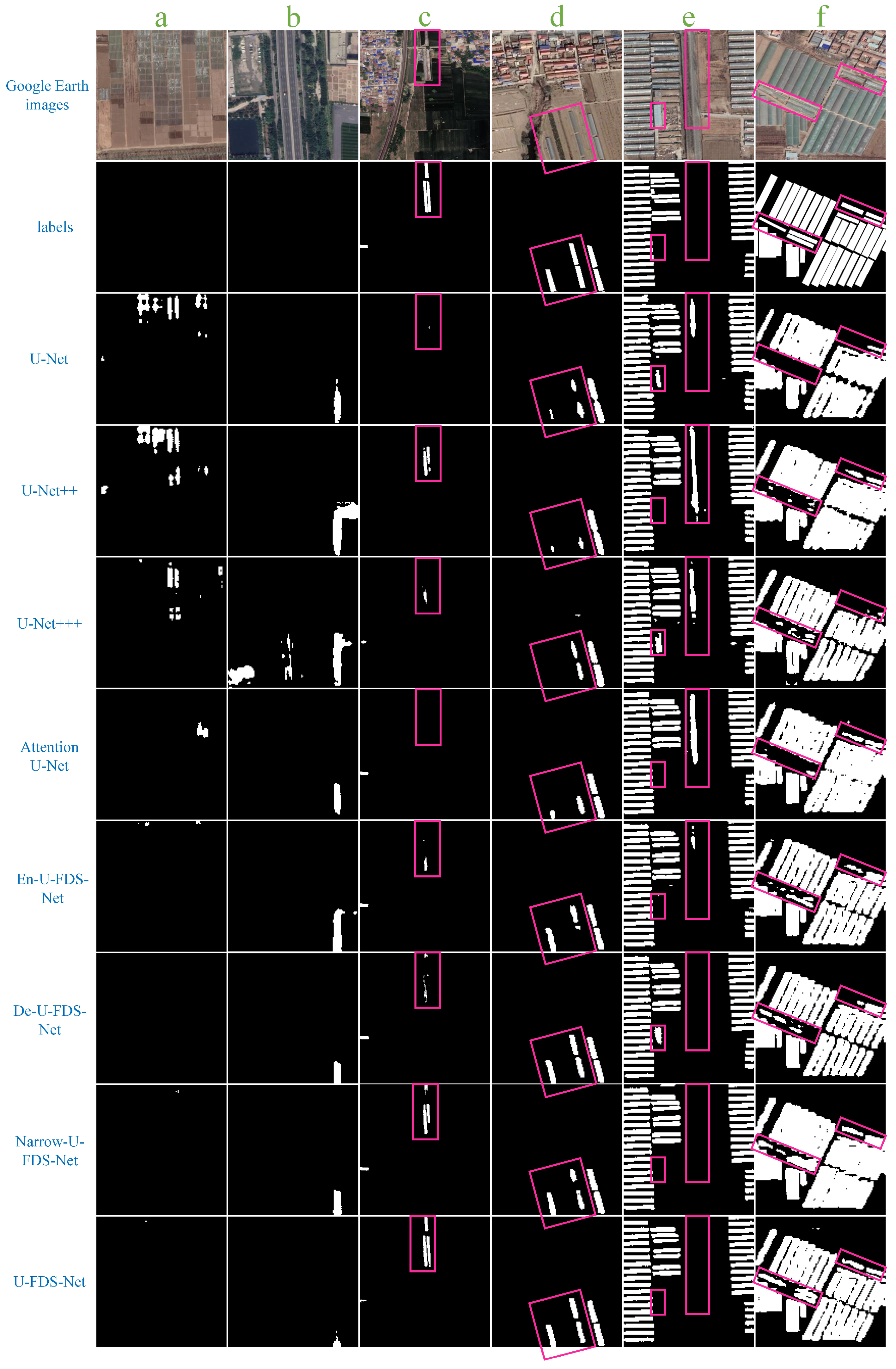
The effects of different models on greenhouse extraction are shown in Figure 10. Figure 10a–c demonstrate the cases where ground objects are very similar to plastic greenhouses but at smaller scales. Our proposed U-FDS Net could determine false positive misclassifications. In Figure 10d, greenhouses are scattered around residential areas and are also easily confused with surrounding objects. The models proposed in this study achieved better performance than the control group, which we believe is due to the stronger overall perception capability of our model, which can explore feature signals of different dilution levels on a full scale, gradually abstract feature maps and perform information integration. Figure 10e shows a situation of densely distributed plastic greenhouses where factory buildings are similar to greenhouses in color, shape and scale, which can also easily cause false positive misclassifications. For such images, the model needs to be able to grasp the spatial information and detailed texture features of the ground objects at the same time. U-FDS Net with a full-scale dense connection structure shows significant advantages. Figure 10f also shows a case of densely distributed plastic greenhouses but with residential areas nearby. The detailed semantics of the image are not well learned by the model of the control group, and our model can obtain more accurate segmentation due to its more delicate perception ability.
4. Discussion
4.1. Advantages
The U-FDS Net proposed in this study is a novel full-scale feature fusion greenhouse extraction deep learning-based method with an advanced architecture of deep supervision and attention mechanisms. As a deep learning approach, it possesses better transferability and feature extraction capabilities compared to traditional remote sensing methods. For example, the spectral index method is often plagued by poor transferability and requires robust professional knowledge. Extracting greenhouses by constructing spectral indices can work well in a small region but may not be applicable in changing seasons and with differences in greenhouse covering materials in different regions when extracting greenhouses over large areas. Using an object-based classification method takes considerable time because the computational cost is high and it can only extract the shallow features of ground objects, which makes it difficult to meet large-scale application needs, while deep learning methods can explore deep, high-level features and benefit from efficient parallel computing on GPU devices.
Compared with the traditional or state-of-the-art network model, U-FDS Net’s novel architecture design can achieve higher segmentation accuracy by learning semantic features of different scales and granularities more fully when dealing with a variety of complex scenarios. Specifically, employing an encoder–decoder structure has become a common paradigm for deploying complex operations in remote sensing semantic segmentation tasks, yet research on network architectures remains in its early stages. Taking EGENet [43] as an example, although it demonstrated the advantage of initiating feature extraction at higher-resolution levels for dense small targets, then, how can further improvement be achieved upon this foundation? Considering that the semantic depth carried by a single encoder–decoder is fixed, U-FDS Net explores the utilization of multiple nested sub-encoder–decoder forms. This can be seen as a higher-order form of a single encoder–decoder, where shallow fine-grained semantics guide deeper high-level features. These features have both global overall information and local detailed information. According to the global information, the most significant appearance performance of the greenhouse can be learned, while the local information provides more details that distinguish the greenhouse from other features. The combination of these two pieces of information reduces false positive misclassifications and provides a more accurate basis for the greenhouse segmentation task. This architectural concept can be applied to other image segmentation tasks; for example, on the Kvasir-SEG public dataset (https://datasets.simula.no/downloads/kvasir-seg.zip, accessed on 10 December 2023), U-FDS Net also achieves the highest mIoU. On the other hand, we strive for low cost, simplicity and practicality. U-FDS Net can achieve higher accuracy with fewer parameters. It does not rely on the user to have robust professional knowledge and only needs to adjust parameters for GPU and TPU hardware with different VRAM and computing power, and it can meet most application scenarios.
4.2. Limitations and Future Perspectives
The U-FDS Net proposed in this study is a fully convolutional image segmentation network. The original intention of our design is to select a relatively common and efficient network structure in the existing research and improve it based on greenhouse data to pursue its accuracy improvement without consuming too much time. However, U-FDS Net does not use self-attention, such as the Swin Transformer [44] and TransUNet [45]. We tested the inference consumption of a single 256 × 256 RGB image on an NVIDIA Tesla V100-SXM2 GPU. The FLOPs, Params and inference time of TransUNet are 32.23 G, 88.91 M and 43.95 ms, respectively, while those of U-FDS Net are 333.31 G, 42.65 M and 27.27 ms, respectively, indicating that the former may have higher GPU VRAM and memory bandwidth requirements in practical applications. The introduction of a transformer structure module in the future may further improve the accuracy of such image-processing tasks, but this may come at the cost of a longer inference speed and higher hardware requirements. On the other hand, we also recommend leveraging multi-source data for performance gains. Specifically, the samples used in this study are 24-bit RGB images with limited perceptual capabilities. Incorporating additional data or bands, such as multi-spectral data sensitive to greenhouses, could further advance the performance boundaries of greenhouse segmentation tasks.
5. Conclusions
Plastic greenhouses are an important part of contemporary facility agriculture. Quickly and accurately extracting plastic greenhouses is important for environmental protection and sustainable development. To accurately monitor the distribution of plastic greenhouses, this paper proposed a new deep learning-based algorithm, named U-FDS Net, combining full-scale dense connections and adaptive deep supervision. This new algorithm aims to more rationally fuse the information obtained from the global, fit exclusive feature representation relationships for different remote sensing images and improve greenhouse extraction accuracy. We tested our model on two high-resolution self-annotated greenhouse datasets at different scales in different study areas. The results show that, compared to U-Net, U-Net++, U-Net+++ and Attention U-Net, our method achieves the best extraction accuracy on both datasets, with performance gains of 0.405–1.592% and 0.602–1.862% in terms of mIoU, respectively, and significantly improves false positive misclassification in greenhouses. Our method enables rapid identification of the spatial distribution of greenhouses, providing technical support for accurate estimation of agricultural output and locating potential environmental pollution caused by greenhouses.
Author Contributions
Conceptualization and writing—original draft preparation, Y.M.; validation, W.Z.; software, W.C. All authors have read and agreed to the published version of the manuscript.
Funding
This research was funded by the National Natural Science Foundation of China, grant number 62261038.
Data Availability Statement
The code will be released at: https://github.com/Jiaaaaa88/2RS.git (accessed on 10 December 2023).
Conflicts of Interest
The authors declare no conflict of interest.
References
- Liu, F.; Zhang, Z.; Shi, L.; Zhao, X.; Xu, J.; Yi, L.; Liu, B.; Wen, Q.; Hu, S.; Wang, X.; et al. Urban expansion in China and its spatial-temporal differences over the past four decades. J. Geogr. Sci. 2016, 26, 1477–1496. [Google Scholar] [CrossRef]
- Nunes, E.M.; Silva, P.S.G. Reforma agrária, regimes alimentares e desenvolvimento rural: Evidências a partir dos territórios rurais do Rio Grande do Norte. Rev. De Econ. E Sociol. Rural. 2023, 61, e232668. [Google Scholar] [CrossRef]
- Zheng, Y.Y.; Kong, J.L.; Jin, X.B.; Wang, X.Y.; Su, T.L.; Zuo, M. CropDeep: The Crop Vision Dataset for Deep-Learning-Based Classification and Detection in Precision Agriculture. Sensors 2019, 19, 1058. [Google Scholar] [CrossRef] [PubMed]
- Stark, J.C. Food production, human health and planet health amid COVID-19. Explor. J. Sci. Health 2021, 17, 179–180. [Google Scholar] [CrossRef]
- Hanan, J.J. Greenhouses: Advanced Technology for Protected Horticulture; CRC Press: Boca Raton, FL, USA, 2017. [Google Scholar]
- Zhang, G.X.; Fu, Z.T.; Yang, M.S.; Liu, X.X.; Dong, Y.H.; Li, X.X. Nonlinear simulation for coupling modeling of air humidity and vent opening in Chinese solar greenhouse based on CFD. Comput. Electron. Agric. 2019, 162, 337–347. [Google Scholar] [CrossRef]
- Novelli, A.; Aguilar, M.A.; Nemmaoui, A.; Aguilar, F.J.; Tarantino, E. Performance evaluation of object based greenhouse detection from Sentinel-2 MSI and Landsat 8 OLI data: A case study from Almeria (Spain). Int. J. Appl. Earth Obs. Geoinf. 2016, 52, 403–411. [Google Scholar] [CrossRef]
- Yang, D.D.; Chen, J.; Zhou, Y.; Chen, X.; Chen, X.H.; Cao, X. Mapping plastic greenhouse with medium spatial resolution satellite data: Development of a new spectral index. ISPRS J. Photogramm. Remote Sens. 2017, 128, 47–60. [Google Scholar] [CrossRef]
- Feng, Q.L.; Niu, B.W.; Chen, B.A.; Ren, Y.; Zhu, D.H.; Yang, J.Y.; Liu, J.T.; Ou, C.; Li, B.G. Mapping of plastic greenhouses and mulching films from very high resolution remote sensing imagery based on a dilated and non-local convolutional neural network. Int. J. Appl. Earth Obs. Geoinf. 2021, 102, 102441. [Google Scholar] [CrossRef]
- Pietro, P. Innovative Material and Improved Technical Design for a Sustainable Exploitation of Agricultural Plastic Film. J. Macromol. Sci. Part D Rev. Polym. Process. 2014, 53, 1000–1011. [Google Scholar]
- Picuno, P.; Sica, C.; Laviano, R.; Dimitrijevic, A.; Scarascia-Mugnozza, G. Experimental tests and technical characteristics of regenerated films from agricultural plastics. Polym. Degrad. Stab. 2012, 97, 1654–1661. [Google Scholar] [CrossRef]
- Picuno, P.; Tortora, A.; Capobianco, R.L. Analysis of plasticulture landscapes in Southern Italy through remote sensing and solid modelling techniques. Landsc. Urban Plan. 2011, 100, 45–56. [Google Scholar] [CrossRef]
- Shi, L.F.; Huang, X.J.; Zhong, T.Y.; Taubenbock, H. Mapping Plastic Greenhouses Using Spectral Metrics Derived From GaoFen-2 Satellite Data. IEEE J. Sel. Top. Appl. Earth Obs. Remote Sens. 2020, 13, 49–59. [Google Scholar] [CrossRef]
- Veettil, B.K.; Xuan, Q.N. Landsat-8 and Sentinel-2 data for mapping plastic-covered greenhouse farming areas: A study from Dalat City (Lam Dong Province), Vietnam. Environ. Sci. Pollut. Res. 2022, 29, 73926–73933. [Google Scholar] [CrossRef] [PubMed]
- Yao, Y.; Wang, S.X. Evaluating the Effects of Image Texture Analysis on Plastic Greenhouse Segments via Recognition of the OSI-USI-ETA-CEI Pattern. Remote Sens. 2019, 11, 231. [Google Scholar] [CrossRef]
- Aguilar, M.A.; Bianconi, F.; Aguilar, F.J.; Fernandez, I. Object-Based Greenhouse Classification from GeoEye-1 and WorldView-2 Stereo Imagery. Remote Sens. 2014, 6, 3554–3582. [Google Scholar] [CrossRef]
- Aguilar, M.A.; Novelli, A.; Nemmaoui, A.; Aguilar, F.J.; González-Yebra, Ó. Optimizing Multiresolution Segmentation for Extracting Plastic Greenhouses from WorldView-3 Imagery; Springer: Cham, Switzerland, 2017. [Google Scholar]
- Balcik, F.B.; Senel, G.; Goksel, C. Object-Based Classification of Greenhouses Using Sentinel-2 MSI and SPOT-7 Images: A Case Study from Anamur (Mersin), Turkey. IEEE J. Sel. Top. Appl. Earth Obs. Remote Sens. 2020, 13, 2769–2777. [Google Scholar] [CrossRef]
- Zhang, P.; Du, P.; Guo, S.; Zhang, W.; Tang, P.; Chen, J.; Zheng, H. A novel index for robust and large-scale mapping of plastic greenhouse from Sentinel-2 images. Remote Sens. Environ. 2022, 276, 113042. [Google Scholar] [CrossRef]
- Wu, C.F.; Deng, J.S.; Wang, K.; Ma, L.G.; Tahmassebi, A.R.S. Object-based classification approach for greenhouse mapping using Landsat-8 imagery. Int. J. Agric. Biol. Eng. 2016, 9, 79–88. [Google Scholar] [CrossRef]
- Ji, L.; Zhang, L.; Shen, Y.; Li, X.; Liu, W.; Chai, Q.; Zhang, R.; Chen, D. Object-Based Mapping of Plastic Greenhouses with Scattered Distribution in Complex Land Cover Using Landsat 8 OLI Images: A Case Study in Xuzhou, China. J. Indian Soc. Remote 2020, 48, 287–303. [Google Scholar] [CrossRef]
- Rostami, A.; Shah-Hosseini, R.; Asgari, S.; Zarei, A.; Aghdami-Nia, M.; Homayouni, S. Active Fire Detection from Landsat-8 Imagery Using Deep Multiple Kernel Learning. Remote Sens. 2022, 14, 992. [Google Scholar] [CrossRef]
- Khoshboresh-Masouleh, M.; Alidoost, F.; Arefi, H. Multiscale building segmentation based on deep learning for remote sensing RGB images from different sensors. J. Appl. Remote Sens. 2020, 14, 034503. [Google Scholar] [CrossRef]
- Ansari, M.; Homayouni, S.; Safari, A.; Niazmardi, S. A New Convolutional Kernel Classifier for Hyperspectral Image Classification. IEEE J. Sel. Top. Appl. Earth Obs. Remote Sens. 2021, 14, 11240–11256. [Google Scholar] [CrossRef]
- Yang, B.; Mao, Y.; Liu, L.; Liu, X.; Ma, Y.; Li, J. From Trained to Untrained: A Novel Change Detection Framework Using Randomly Initialized Models With Spatial-Channel Augmentation for Hyperspectral Images. IEEE Trans. Geosci. Remote Sens. 2023, 61, 1–14. [Google Scholar] [CrossRef]
- Aghdami-Nia, M.; Shah-Hosseini, R.; Rostami, A.; Homayouni, S. Automatic coastline extraction through enhanced sea-land segmentation by modifying Standard U-Net. Int. J. Appl. Earth Obs. Geoinf. 2022, 109, 102785. [Google Scholar] [CrossRef]
- Yang, B.; Qin, L.; Liu, J.; Liu, X. UTRNet: An Unsupervised Time-Distance-Guided Convolutional Recurrent Network for Change Detection in Irregularly Collected Images. IEEE Trans. Geosci. Remote Sens. 2022, 60, 1–16. [Google Scholar] [CrossRef]
- Ranjbar, S.; Zarei, A.; Hasanlou, M.; Akhoondzadeh, M.; Amini, J.; Amani, M. Machine learning inversion approach for soil parameters estimation over vegetated agricultural areas using a combination of water cloud model and calibrated integral equation model. J. Appl. Remote Sens. 2021, 15, 018503. [Google Scholar] [CrossRef]
- Zarei, A.; Hasanlou, M.; Mahdianpari, M. A comparison of machine learning models for soil salinity estimation using multi-spectral earth observation data. ISPRS Ann. Photogramm. Remote Sens. Spatial Inf. Sci. 2021, V-3-2021, 257–263. [Google Scholar] [CrossRef]
- Zhou, Z.H.; Feng, J. Deep Forest: Towards an Alternative to Deep Neural Networks. In Proceedings of the 26th International Joint Conference on Artificial Intelligence (IJCAI), Melbourne, Australia, 19–25 August 2017; pp. 3553–3559. [Google Scholar]
- Ball, J.E.; Anderson, D.T.; Chan, C.S. Comprehensive survey of deep learning in remote sensing: Theories, tools, and challenges for the community. J. Appl. Remote Sens. 2017, 11, 42609. [Google Scholar] [CrossRef]
- Shelhamer, E.; Long, J.; Darrell, T. Fully Convolutional Networks for Semantic Segmentation. IEEE Trans. Pattern Anal. Mach. Intell. 2017, 39, 640–651. [Google Scholar] [CrossRef]
- Ronneberger, O.; Fischer, P.; Brox, T. U-Net: Convolutional Networks for Biomedical Image Segmentation; Springer International Publishing: Berlin/Heidelberg, Germany, 2015. [Google Scholar]
- Chen, L.C.; Papandreou, G.; Kokkinos, I.; Murphy, K.; Yuille, A.L. DeepLab: Semantic Image Segmentation with Deep Convolutional Nets, Atrous Convolution, and Fully Connected CRFs. IEEE Trans. Pattern Anal. Mach. Intell. 2018, 40, 834–848. [Google Scholar] [CrossRef]
- Guo, X.; Li, P. Mapping plastic materials in an urban area: Development of the normalized difference plastic index using WorldView-3 superspectral data. ISPRS J. Photogramm. Remote Sens. 2020, 169, 214–226. [Google Scholar] [CrossRef]
- Zhong, C.; Ting, Z.; Chao, O. End-to-End Airplane Detection Using Transfer Learning in Remote Sensing Images. Remote Sens. 2018, 10, 139. [Google Scholar]
- Li, M.; Zhang, Z.J.; Lei, L.P.; Wang, X.F.; Guo, X.D. Agricultural Greenhouses Detection in High-Resolution Satellite Images Based on Convolutional Neural Networks: Comparison of Faster R-CNN, YOLO v3 and SSD. Sensors 2020, 20, 4938. [Google Scholar] [CrossRef] [PubMed]
- Ma, A.L.; Chen, D.Y.; Zhong, Y.F.; Zheng, Z.; Zhang, L.P. National-scale greenhouse mapping for high spatial resolution remote sensing imagery using a dense object dual-task deep learning framework: A case study of China. ISPRS J. Photogramm. Remote Sens. 2021, 181, 279–294. [Google Scholar] [CrossRef]
- Chen, W.; Xu, Y.M.; Zhang, Z.; Yang, L.; Pan, X.B.; Jia, Z. Mapping agricultural plastic greenhouses using Google Earth images and deep learning. Comput. Electron. Agric. 2021, 191, 106552. [Google Scholar] [CrossRef]
- Niu, B.W.; Feng, Q.L.; Chen, B.; Ou, C.; Liu, Y.M.; Yang, J.Y. HSI-TransUNet: A transformer based semantic segmentation model for crop mapping from UAV hyperspectral imagery. Comput. Electron. Agric. 2022, 201, 107297. [Google Scholar] [CrossRef]
- Huang, H.M.; Lin, L.F.; Tong, R.F.; Hu, H.J.; Zhang, Q.W.; Iwamoto, Y.; Han, X.H.; Chen, Y.W.; Wu, J. UNET 3+: A full-scale connected unet for medical image segmentation. In Proceedings of the IEEE International Conference on Acoustics, Speech, and Signal Processing, Barcelona, Spain, 4–8 May 2020; pp. 1055–1059. [Google Scholar]
- Zhou, Z.; Siddiquee, M.M.R.; Tajbakhsh, N.; Liang, J. UNet++: A Nested U-Net Architecture for Medical Image Segmentation. In Proceedings of the Deep Learning in Medical Image Analysis: 4th International Workshop (DLMIA 2018), and Multimodal Learning for Clinical Decision Support, International Workshop and 8th International Workshop, Held in Conjunction with MICCAI 2018 (ML-CDS 2018), Granada, Spain, 20 September 2018; Volume 11045, pp. 3–11. [Google Scholar] [CrossRef]
- Chen, W.; Wang, Q.; Wang, D.; Xu, Y.; He, Y.; Yang, L.; Tang, H. A lightweight and scalable greenhouse mapping method based on remote sensing imagery. Int. J. Appl. Earth Obs. Geoinf. 2023, 125, 103553. [Google Scholar] [CrossRef]
- Liu, Z.; Lin, Y.; Cao, Y.; Hu, H.; Wei, Y.; Zhang, Z.; Lin, S.; Guo, B. Swin Transformer: Hierarchical Vision Transformer using Shifted Windows. In Proceedings of the IEEE/CVF International Conference on Computer Vision (ICCV), Montreal, BC, Canada, 11–17 October 2021. [Google Scholar]
- Chen, J.; Lu, Y.; Yu, Q.; Luo, X.; Adeli, E.; Wang, Y.; Lu, L.; Yuille, A.L.; Zhou, Y. TransUNet: Transformers Make Strong Encoders for Medical Image Segmentation. arXiv 2021, arXiv:2102.04306. [Google Scholar]
Figure 1.
U-FDS Net structure diagram. On the far left is a downsampling coding structure based on max pooling. To the right of the encoder is a series of full-scale densely connected structures, where i indices the downsampling layer along the encoder, j represents the j-th column in each row, Fi j represents the cascaded result of the i-th row and the j-column obtained by the fusion of full-scale dense connections, and Xi j represents the feature map stack of the cascaded result of the corresponding position after two convolutions. The top of the network is the deeply supervised result of each nested structure. The network assigns weights to each branch by itself during training, and finally, pixel-level addition and fusion are performed according to the iterative weights to obtain the final result.

Figure 2.
Full-scale densely connected structure of U-FDS Net (taking the third row and third column as an example).
Figure 2.
Full-scale densely connected structure of U-FDS Net (taking the third row and third column as an example).

Figure 3.
Common deep supervision structures of U-FDS Net.

Figure 4.
En-U-FDS Net structure diagram. The right side is the deep supervision scheme with step-by-step upsampling.
Figure 4.
En-U-FDS Net structure diagram. The right side is the deep supervision scheme with step-by-step upsampling.

Figure 5.
De-U-FDS Net structure diagram. The right side is the deep supervision scheme of far-hop upsampling.
Figure 5.
De-U-FDS Net structure diagram. The right side is the deep supervision scheme of far-hop upsampling.

Figure 6.
Schematic diagram of the study area and the basic shape of a plastic greenhouse in the study area. (a,b) are the different shapes of the greenhouse in the high-resolution remote sensing image, and (c) is a close-up view of a plastic greenhouse.
Figure 6.
Schematic diagram of the study area and the basic shape of a plastic greenhouse in the study area. (a,b) are the different shapes of the greenhouse in the high-resolution remote sensing image, and (c) is a close-up view of a plastic greenhouse.

Figure 7.
Main plastic greenhouse types and their labels in the study area. Among them, (a) is a white plastic greenhouse distributed near residential areas; (b) is a light green densely distributed plastic greenhouse; (c) is a green-covered plastic greenhouse; and (d) is a black-covered plastic greenhouse because the top is covered with a shading cloth.

Figure 8.
Overall flowchart of extracting plastic greenhouses in this study.

Figure 9.
Precision comparison of each model in different datasets. In each dataset, the four models on the left are used for comparison, and the four on the right are the models proposed in this study.
Figure 9.
Precision comparison of each model in different datasets. In each dataset, the four models on the left are used for comparison, and the four on the right are the models proposed in this study.

Figure 10.
The results of different models. Among them, (a,b) are instances where there are no greenhouses at all, (c,d) are instances where only a few greenhouses exist, and (e,f) are instances where greenhouses are densely distributed; the first row is the original remote sensing images, the second row is the corresponding labels, and then each row corresponds to the greenhouse detection results of each model.


Table 1.
Information on the self-annotated plastic greenhouse dataset.
| Region | Size | Training | Evaluation | Test | Total |
|---|---|---|---|---|---|
| Shandong | 512 × 512 | 4849 | 606 | 606 | 6061 |
| Beijing | 256 × 256 | 5472 | 684 | 684 | 6840 |
Table 2.
Binary confusion matrix.
| Confusion Matrix | Predict | ||
|---|---|---|---|
| True | False | ||
| Real | True | TP (True positive) | FN (False negative) |
| False | FP (False positive) | TN (True negative) | |
Table 3.
The number of parameters and segmentation results of each model.
| Model | Params | Dataset | |
|---|---|---|---|
| Shandong | Beijing | ||
| U-Net | 12.77 M | 88.9266 | 92.4881 |
| U-Net++ | 44.99 M | 89.3119 | 92.7878 |
| U-Net+++ | 25.72 M | 90.1137 | 93.0096 |
| Attention U-Net | 38.25 M | 89.3293 | 93.7484 |
| En-U-FDS Net | 37.36 M | 90.0888 | 94.0418 |
| De-U-FDS Net | 37.36 M | 90.1263 | 94.0531 |
| Narrow-U-FDS Net | 10.67 M | 90.1381 | 94.1244 |
| U-FDS Net | 42.65 M | 90.5190 | 94.3499 |
Disclaimer/Publisher’s Note: The statements, opinions and data contained in all publications are solely those of the individual author(s) and contributor(s) and not of MDPI and/or the editor(s). MDPI and/or the editor(s) disclaim responsibility for any injury to people or property resulting from any ideas, methods, instructions or products referred to in the content. |
© 2023 by the authors. Licensee MDPI, Basel, Switzerland. This article is an open access article distributed under the terms and conditions of the Creative Commons Attribution (CC BY) license (https://creativecommons.org/licenses/by/4.0/).
Share and Cite
MDPI and ACS Style
Mo, Y.; Zhou, W.; Chen, W. Extracting Plastic Greenhouses from Remote Sensing Images with a Novel U-FDS Net. Remote Sens. 2023, 15, 5736. https://doi.org/10.3390/rs15245736
AMA Style
Mo Y, Zhou W, Chen W. Extracting Plastic Greenhouses from Remote Sensing Images with a Novel U-FDS Net. Remote Sensing. 2023; 15(24):5736. https://doi.org/10.3390/rs15245736
Chicago/Turabian StyleMo, Yan, Wanting Zhou, and Wei Chen. 2023. "Extracting Plastic Greenhouses from Remote Sensing Images with a Novel U-FDS Net" Remote Sensing 15, no. 24: 5736. https://doi.org/10.3390/rs15245736
Note that from the first issue of 2016, this journal uses article numbers instead of page numbers. See further details here.