Article

Analysis of Illumination Conditions in the Lunar South Polar Region Using Multi-Temporal High-Resolution Orbital Images

1
State Key Laboratory of Remote Sensing Science, Aerospace Information Research Institute, Chinese Academy of Sciences, Beijing 100101, China
2
University of Chinese Academy of Sciences, Beijing 100039, China
3
Center for Excellence in Comparative Planetology, Chinese Academy of Sciences, Hefei 230026, China
4
Beijing Aerospace Control Center (BACC), Beijing 100094, China
5
Key Laboratory of Earth and Planetary Physics, Institute of Geology and Geophysics, Chinese Academy of Sciences, Beijing 100029, China
*
Author to whom correspondence should be addressed.
Remote Sens. 2023, 15(24), 5691; https://doi.org/10.3390/rs15245691
Submission received: 27 September 2023 / Revised: 8 December 2023 / Accepted: 9 December 2023 / Published: 11 December 2023
(This article belongs to the Special Issue Remote Sensing and Photogrammetry Applied to Deep Space Exploration)

Abstract

:
The illumination conditions of the lunar south pole region are complex due to the rugged terrain and very low solar elevation angles, posing significant challenges to the safety of lunar landing and rover explorations. High-spatial and temporal-resolution analyses of the illumination conditions in the south pole region are essential to support mission planning and surface operations. This paper proposes a method for illumination condition analysis in the lunar pole region using multi-temporal high-resolution orbital images with a pre-selected landing area of Chang’E-7 as the study area. Firstly, a database of historical multi-temporal high-resolution (0.69–1.97 m/pixel) orbital images, with associated image acquisition time, solar elevation angle, and azimuth angle, is established after preprocessing and registration. Secondly, images with the nearest solar elevation and azimuth at the planned time for mission operations are retrieved from the database for subsequent illumination condition analysis and exploration support. The differences in the actual solar positions at the mission moments from that of the nearest sun position image are calculated and their impact on illumination conditions is evaluated. Experimental results of the study area demonstrate that the constructed image database and the proposed illumination analysis method using multi-temporal images, with the assistance of DEM in a small number of cases, can effectively support the mission planning and operations for the Chang’E-7 mission in the near future.

1. Introduction

The lunar south pole, with its abundant resources (e.g., solar energy resources in permanently illuminated regions (PIR), potential water ice in permanently shadowed regions (PSR)) and favorable scientific value, has become a prime area for exploration activities to be conducted by various countries [1]. Both NASA’s Artemis mission and CNSA’s Chang’E-7 mission plan to carry out lunar lander reconnaissance and exploration at the lunar south pole region [2,3,4]. The Moon has an orbital period of approximately 27 days, with most regions experiencing about 14 days of sunlight followed by a similar length of darkness. This prolonged day–night cycle presents challenges for lunar missions and human habitation on the Moon’s surface. Previous studies have indicated that certain high-elevation areas such as the edges of impact craters, mountain peaks, and ridges in the polar regions receive ample sunlight and exhibit more stable temperatures, making them suitable for surface exploration and the establishment of lunar bases [5]. Due to the small inclination angle (1.54°) between the lunar equatorial plane and the ecliptic plane and rugged terrain, the lunar south pole contains numerous PSR with extremely low surface temperatures [6], which have the potential to harbor water ice and other volatile substances. In the 1960s, the existence of water ice deposits in these PSR was first suggested [7], and lots of subsequent remote sensing observations and research also gave evidence of the existence of water ice [8]. Water ice not only serves as a crucial resource for future human life and work on the lunar surface, but also poses an important scientific question regarding its origin.
Exploration missions to the lunar poles require a thorough understanding of the illumination conditions in the polar regions [9]. They play a crucial role in environmental analyses for lunar polar explorations and in selecting suitable locations for lunar research stations [10,11,12]. Depending on the data sources used, analysis of lunar polar illumination can be categorized into two approaches: analysis based on the Digital Elevation Model (DEM) and analysis based on images. DEM-based illumination analysis is limited by the accuracy and resolution of the DEM. Particularly for mission planning involving lunar rovers, its reliability and precision need further validation. Image-based illumination analysis, on the other hand, provides precise analysis of the illumination conditions with the resolution of the image at the time of image acquisition. However, the temporal resolution is usually limited by the frequency and periodicity of image acquisitions. With the increasing acquisition of high-resolution images, the number of revisits has increased, especially in polar regions, which makes the multi-temporal images available for illumination condition analysis.
To address the demand for high-precision illumination environment analysis in future exploration missions, this research proposes a method for lunar south pole illumination analysis using multi-temporal high-resolution remote sensing imagery. By taking full advantage of high image resolution and direct analysis of illumination conditions, as well as utilizing the multi-coverage and multi-temporal characteristics of existing orbiters, the research aims to conduct a high-precision illumination environment analysis in specific areas of the south pole. The feasibility and effectiveness of using multiple coverage images to support illumination analysis for lunar polar exploration are investigated.
The rest of the paper is organized as follows. Section 2 briefly reviews previous research relevant to this paper, including illumination analysis research based on DEM and imagery. The study area and data are introduced in Section 3. Section 4 describes the methodology for constructing a high-resolution lunar polar image dataset and performing geographical registration and illumination analysis. Section 5 presents the results and discussions of the illumination condition analysis at the study area, which is a pre-selected landing area for the Chang’E-7 mission. Section 6 gives some conclusions of this research.

2. Related Work

DEM-based illumination condition analyses have been performed and widely used in many studies. In the 1990s, Margot et al. [13] conducted simulations of illumination conditions using lunar DEM obtained from ground-based radar observations. Subsequently, with the launch of JAXA’s Kaguya spacecraft carrying a laser altimeter, detailed topographic data of the lunar polar regions became available, leading to an increasing focus on lunar polar illumination studies based on DEM [14,15,16]. Noda et al. [16] used the laser altimeter data from Kaguya to generate a polar DEM with a resolution of 470 m/pixel. They simulated the polar illumination conditions for a duration of 2000 days based on this DEM and compared it with images from the Clementine mission, verifying the reliability of DEM-based illumination simulations. NASA’s Lunar Reconnaissance Orbiter (LRO), equipped with the Lunar Orbiter Laser Altimeter (LOLA), subsequently obtained a large amount of high-precision lunar data [17,18]. Mazarico et al. [19] used over 2600 LOLA tracks of point cloud data to construct a polar DEM with a resolution of 240 m/pixel and calculated the illumination ratios of the lunar polar regions using the maximum terrain height angle method. De Rosa et al. [20] further improved the resolution of the DEM to 40 m/pixel and applied it to site selection for future lunar landing missions by the European Space Agency. Gläser et al. [21] combined the LOLA DEM with photogrammetric techniques to achieve an overall resolution of 20 m/pixel and a local resolution of 2 m/pixel, enabling a detailed analysis of the illumination conditions at potential landing sites in the south pole region.
The above-mentioned analysis of lunar south pole illumination based on DEM primarily utilizes the horizon method [19]. This method involves calculating the horizon for each grid in the research area using the DEM, and constructing a horizon database. Subsequently, the database can be used to generate illumination maps for different periods using the solar ephemerides, or to obtain simulated binary images representing the lighting conditions. One limitation of this method is the huge computational cost of constructing the horizon database, making it very time-consuming. So some researchers have started exploring approaches such as multi-threading, GPU acceleration, and construction of pyramidal horizon databases to simplify the computations and reduce processing time [20,22]. Using DEM for illumination condition analysis can not only simulate the illumination image and extract the shadow area at any time, but also can calculate the average illumination for a period of time, and extract the permanent lighting and shadowed areas. However, this method is limited by the resolution and accuracy of the DEM. Existing global or regional DEM products of the Moon have limited resolution (a hundred meters to tens of meters), and the accuracy assessment of them is difficult [23]. Currently, the highest resolution DEM of the lunar south pole is a 5 m/pixel resolution product derived from LOLA data [24,25]. The shape from shading [26,27] and deep learning [28,29] methods can be used to produce a DEM with the same resolution as the image from a single high-resolution image. Liu et al. proposed a generative adversarial network (GAN) called LDEMGAN, which generates pixel-scale lunar DEM from monocular LROC NAC imagery aided by existing low-resolution DEM [28]. Tao et al. proposed a network based on GAN for fast reconstruction of DEM from images [29]. However, the lunar polar region has a low solar elevation angle, which results in poor image quality and a lot of shadow coverage in the image. This restricts the accuracy of DEM generated from single imagery. Overall, there are still limitations when using this DEM to analyze the illumination conditions in polar regions for supporting lunar landing and rover operation.
The illumination conditions can be directly observed using high-resolution images. The spatial accuracy depends on the resolution of the images, which is always higher than DEM, while the temporal resolution is related to the orbital period. For example, early missions like Clementine only obtained polar illumination data for 2.5 lunar days due to their short mission lifetimes. Previous studies have explored the illumination conditions in the lunar polar regions using LRO Camera (LROC) Wide-Angle Camera (WAC) images. Speyerer and Robinson [30] surveyed the lighting conditions in the lunar polar regions using approximately 7800 images from the LROC WAC. They constructed image-based illumination maps and created movie sequences to depict lunar lighting variations. The LRO team has also produced numerous mapping products for the lunar south pole using LROC Narrow-Angle Cameras (NAC) images. These include uncontrolled 1 m/pixel resolution mosaics of the lunar south pole and maps of permanent shadowed regions derived from long-exposure images [31,32]. These studies demonstrate that LROC images have extensive coverage of the lunar polar regions, providing images under various lighting conditions, which is highly relevant for lunar polar illumination research.
In the 21st century, several lunar orbital missions have observed the polar regions, including JAXA’s Kaguya, NASA’s LRO, and ISRO’s Chandrayaan-1 and Chandrayaan-2, as well as CNSA’s Chang’E-1 and Chang’E-2 [33]. In particular, the LRO mission has achieved sub-meter-level resolution with its long-term observations and extensive image coverage in the polar regions. It operates in a polar orbit around the Moon and provides images under different illumination conditions, which is highly suitable for lunar polar lighting studies.

3. Study Area and Data
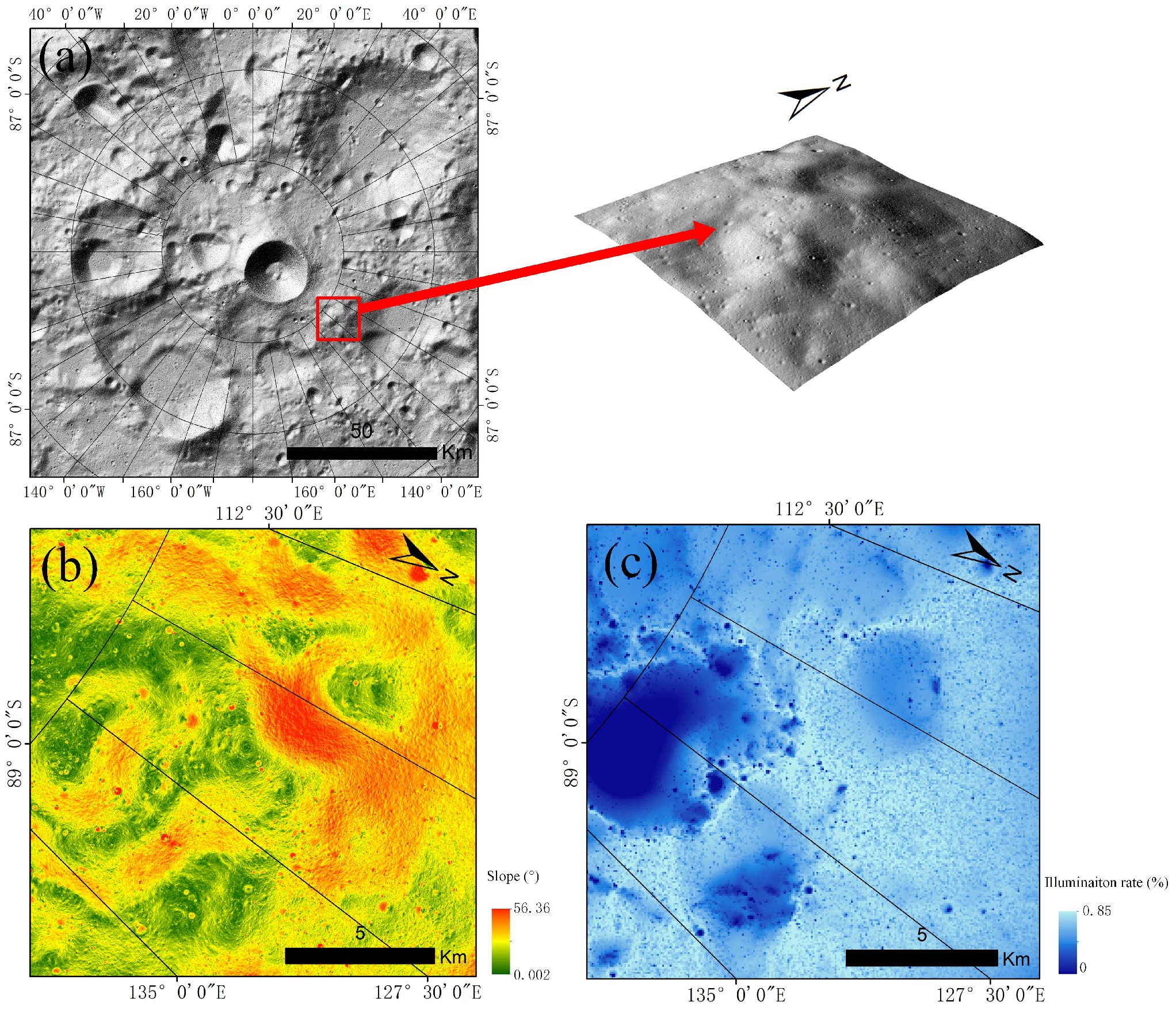
3.1. Study Area

In this research, a pre-selected landing area of Chang’E-7 southeast of Shackleton impact crater (Figure 1), a popular landing area studied in many studies [9,19,34,35], was selected as the study area of this research. This region with an approximate size of 3 km × 3 km features a flat plateau. The average slope is about 6°, and the average illumination is approximately 0.35. Some parts of the plateau experience relatively long periods of illumination (>80%). The favorable topographic and illumination conditions make it an ideal landing area for rover traversing and exploration.

3.2. Data

  • Multi-temporal high-resolution orbital images
Thorough investigation of existing orbital optical images, LROC NAC images are selected to construct the image database, supplemented by Terrain Mapping Camera-2 (TMC-2) images from Chandrayaan-2. The NAC is composed of NAC-L and NAC-R, each has a focal length of 700 mm and a field of view of 2.85 degrees. Each camera can capture a swath width of 2.5 km with a resolution of 0.5 m for panchromatic image when the spacecraft is at an orbital altitude of 50 km. The NAC image has a spatial resolution ranging from 0.5 m to 2 m with different orbital altitudes. One of the primary objectives of LRO is to assess features at the meter-scale and smaller resolutions in polar regions, aiming to survey polar resources and conduct safety analyses for potential landing sites on the Moon [36]. Therefore, the spacecraft is designed to operate in a lunar polar orbit, which provides the highest revisit frequency over the polar regions, enabling LROC NAC image to have extensive high-resolution repetitive coverage in the lunar polar regions. In this research, 226 LROC NAC images were selected and downloaded from the PDS Geosciences Node Lunar Orbital Data Explorer website (https://ode.rsl.wustl.edu/moon/index.aspx, accessed on 11 September 2023). The images were acquired from July 2009 to September 2020, with resolutions from 0.69 m/pixel to 1.97 m/pixel, azimuth angles from 0.99° to 359.24°, and elevation angles from −2.57° to 2.73°.
TMC-2 of Chandrayaan-2 can provide high-resolution images of the Moon’s polar regions. TMC-2 is configured to provide panchromatic images, and stereo triplets at 5 m/pixel spatial resolution from a 100 km circular orbit around the Moon for preparing detailed DEM of the complete lunar surface [37,38]. To supplement the LROC NAC images, 5 TMC-2 images were selected and downloaded from the Indian Space Science Data Center website (https://pradan.issdc.gov.in/ch2/protected/payload.xhtml, accessed on 11 September 2023). These images were acquired from 11 November 2021, and 12 November 2021, with resolutions of 5 m/pixel, azimuth angles from 318.78° to 333.02°, and elevation angles from 0.59° to 0.72°.
2.
LOLA DEM (LDEM)
LOLA is a laser altimetry system carried on the LRO spacecraft. Its main objective is to establish a precise geodetic framework and provide a unified geodetic reference for other lunar data. With an orbit reconstruction error of around 7 m, LOLA provides the highest resolution and best accuracy lunar surface topographic data available [39].
An improved 5 m/pixel LOLA DEM (https://pgda.gsfc.nasa.gov/products/78, accessed on 11 September 2023), corrected through orbit self-alignment, was utilized in this research. The orbit self-alignment process reduced the orbit error by more than 10 times; the LDEM surface height uncertainty has typical RMS values of ~0.30 to 0.50 m, significantly minimizing terrain artifacts caused by orbit errors and noises [25].

4. Method

Based on the multi-temporal high-resolution orbital images, this paper proposes an analysis method for the lunar south pole illumination conditions. It fully utilizes the high-resolution and multi-temporal coverage characteristics of the images to conduct high-spatiotemporal-resolution analyses of the illumination environment in specific regions of the lunar south pole. The overall workflow of the method is illustrated in Figure 2.
Firstly, multi-temporal images of the study area are selected, radiometrically processed, geometrically processed, and registered (see Section 4.1.1 for details). Then, according to the image acquisition time and area, the solar elevation angle and azimuth angle at the time of image acquisition are calculated (see Section 4.1.2 for details). After that, a database including image acquisition time, solar elevation angle and azimuth angle, and image storage location is established for subsequent illumination condition studies and exploration support. During mission execution, according to the time required for mission planning, images with the nearest solar elevation and azimuth angle are retrieved from the database for subsequent usage. The differences in the actual solar positions at the mission moments from that of the nearest sun position image are calculated and their impact on illumination conditions is evaluated using DEM-based illumination simulation (see Section 5.2 for details). Finally, comprehensive illumination analysis is performed at the study area using high-resolution multi-temporal images, with the assistance of the DEM in some cases.

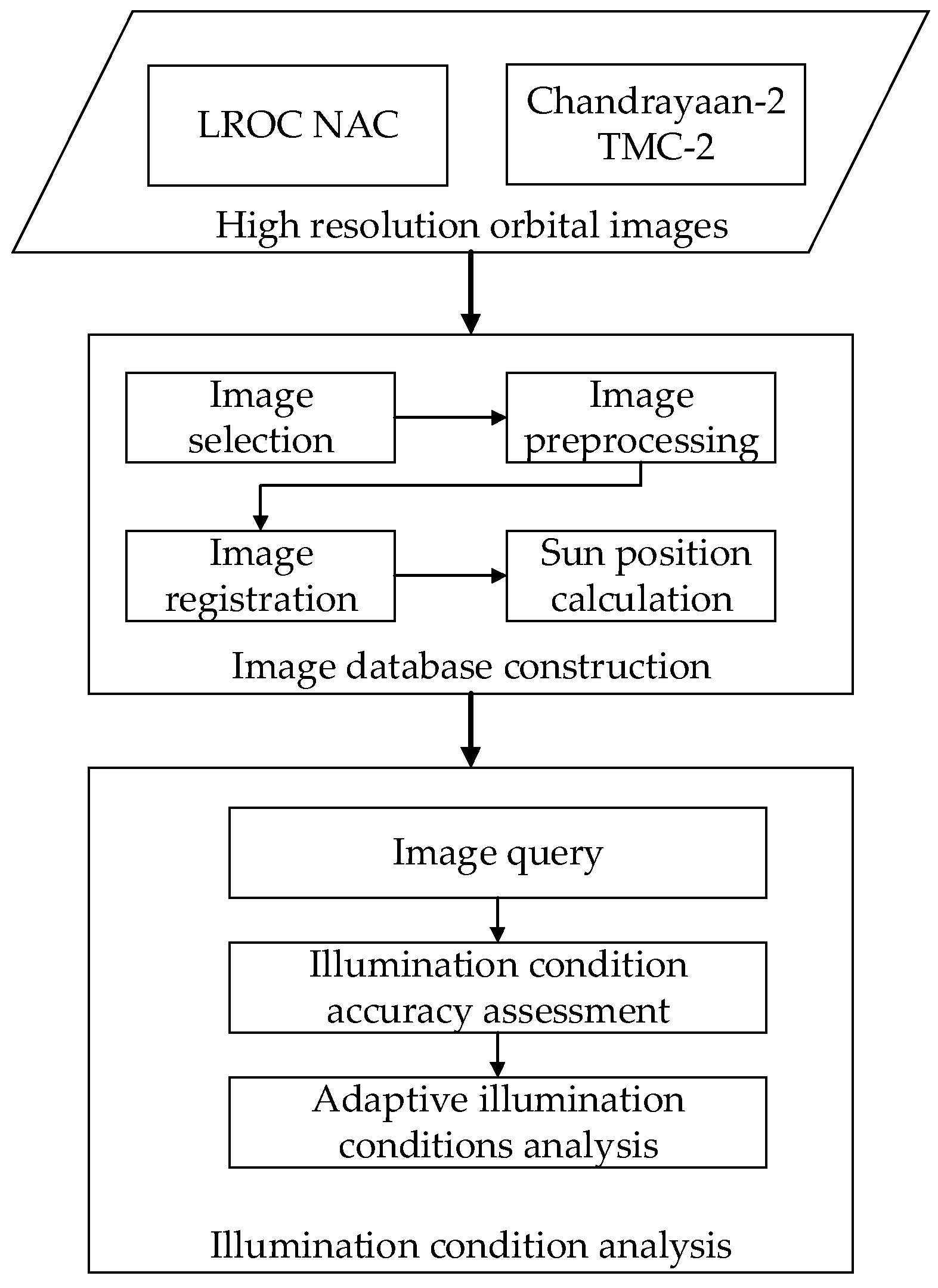
4.1. Image Database Construction

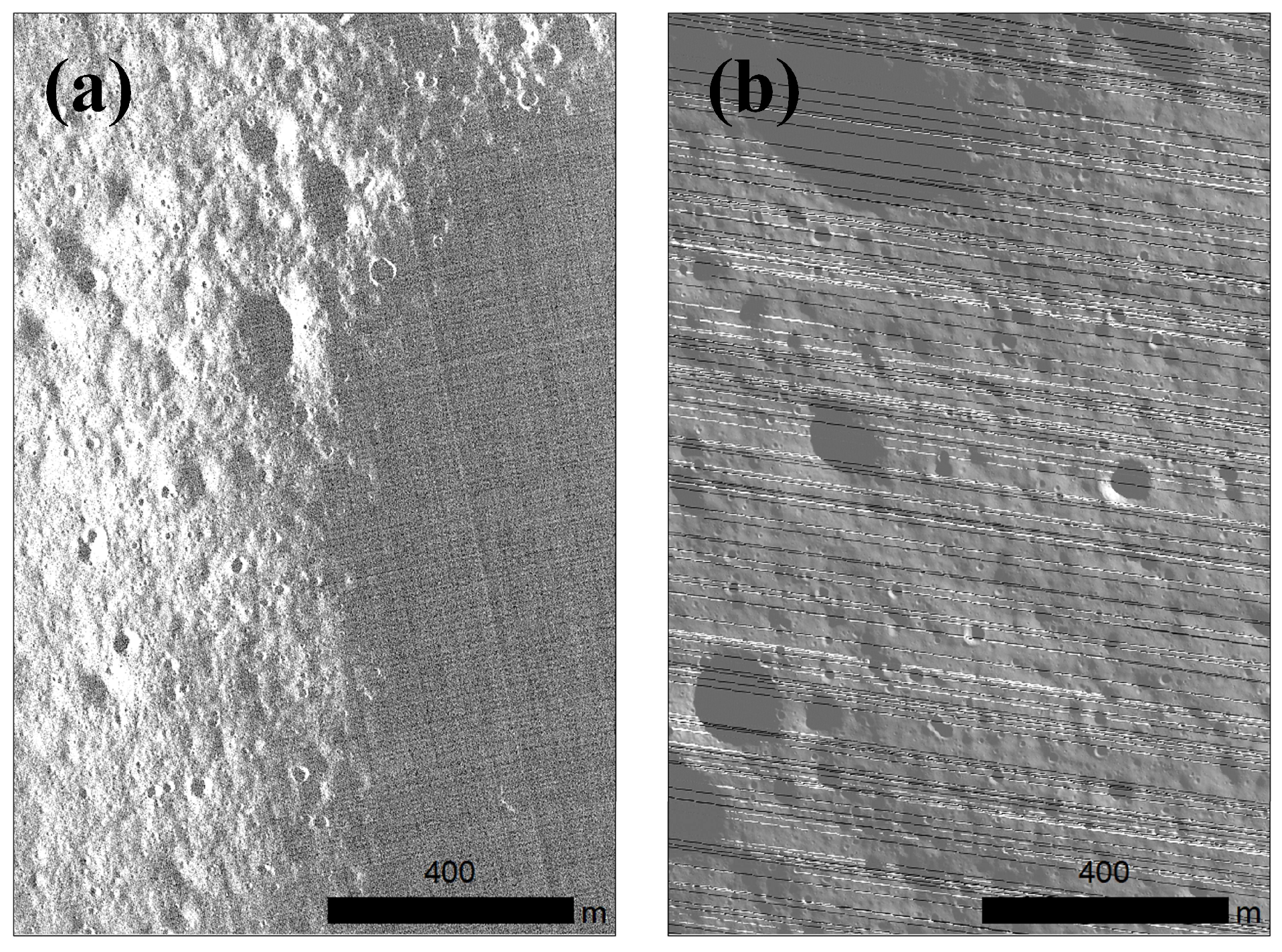
4.1.1. Image Preprocessing and Registration

Firstly, muti-temporal images of the study area were downloaded. Then, images with excessive shadow areas and significant noises (Figure 3 for example) were excluded through visual interpretation. Subsequently, the selected images underwent image preprocessing, orthorectification, and image registration.
The ISIS (Integrated System for Imagers and Spectrometers) [40,41] software was used for image preprocessing and orthorectification. Taking LROC NAC image processing as an example, the downloaded raw image data in the IMG format were first converted to the ISIS-readable CUB format using the lronac2isis command. The Spiceinit command was then used to read the relevant kernel files and construct the camera model. The 1ronaccal command was used to perform basic radiometric calibration, effectively eliminating some vertical striping issues in the images. The lronacecho command was applied to remove the echo noise present in the image, which was caused by the high-speed motion of the NAC detector during image acquisition. After processing, the boundaries of features in the images were enhanced and became clearer. Finally, the cam2map command was used for orthorectification at the south-polar stereographic projection. For TMC-2, orthoimages can be downloaded directly from the Indian Space Science Data Center website (https://pradan.issdc.gov.in/ch2/protected/payload.xhtml, accessed on 11 September 2023).
Due to the presence of orbit and attitude measurement errors, there is geolocation deviation among the multi-temporal images of the same area [42,43]. The tens-of-meter-level positioning errors cause noticeable displacement of geologic features (e.g., craters) and significantly affect the subsequent analysis. In order to perform joint processing, the image also needs to be registered with DEM. Due to the very different azimuth angles, the visual appearances of the multi-temporal images are significantly different (see examples in Figure 4), making the image matching and registration very difficult in the lunar polar regions. To tackle this problem, we propose a matching strategy for the high-resolution images with different illumination conditions using the DEM as a bridge.
Firstly, the muti-temporal images are divided into several groups based on their azimuth angles in a way that the lighting differences among the images within the group do not affect the subsequent image matching. Within each group, the image with the highest sun elevation angle and the least shadow coverage is selected as the reference image of the group. This image is chosen because it contains visually richest information within the group. Next, the reference images of all groups are matched with the DEM by using the DEM-simulated illumination images (see Section 4.1.3 for details), which are generated based on solar azimuth and elevation angles of the reference images for each group. The DEM-simulated illumination images are much similar to the actual orbital images, making it much easier to match the reference images to the DEM. SIFT (Scale-Invariant Feature Transform) feature matching [44] is used to match the reference images with their corresponding simulated illumination images. SIFT feature matching is a local feature detection algorithm based on scale, rotation, and affine invariant features, which can maintain a certain degree of stability against light, noise, and viewing angle variations. An outlier rejection algorithm based on Random Sample Consensus (RANSAC) [45] and affine transformation is employed to eliminate mismatched points and retain correctly matched points. The process of RANSAC is as follows: First, several sample points in the sample set are randomly selected to calculate the parameters of an affine transformation model. Second, other sample points are calculated using the model parameters, and whether or not they are “inner points” in line with the model is judged according to the set threshold value. If not, they are divided into “outer points”, and the set of inner points and the number of inner points is recorded. Then, the algorithm repeats the above steps, selects the inner point set with the largest number of inner points, and recalculates the parameters of the affine transformation model. SIFT feature matching and RANSAC are open-source algorithms.
The reference images are registered to the DEM using affine transformations, achieving sub-pixel-level registration precision. Other images in each group are registered to the reference image of the group using SIFT feature matching, thus completing the registration of all images and the DEM.

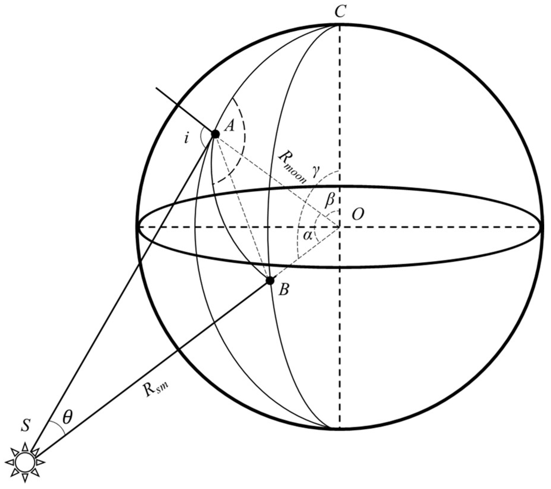
4.1.2. Sun Position Calculation

Due to the wide longitudinal span (could be tens to a hundred degrees) of the polar region images, there is significant variation in the solar azimuth angle within the study area. Estimating the solar azimuth at a specific location in the image based on the solar azimuth at the image center (which is provided in the image header) is not accurate. Therefore, it is necessary to calculate the solar azimuth for any specific location within the study area.
In this research, SpiceyPy, which is a Python version of the SPICE toolkit [46], was used to calculate the precise location of the subsolar point at a specific moment using the DE440 ephemeris [47]. The coordinates were transformed into the lunar body’s fixed coordinate system. Using spherical geometry methods, the elevation angle and azimuth angle at different observation points were calculated.
Based on the geometric position information of the Moon and the Sun (Figure 5), the elevation angle and azimuth angle at different times can be calculated. The elevation angle can be obtained using the following formula [48],
δ = π 2 ( α + θ )
α = arccos [ sin φ A sin φ d + cos φ A cos φ d cos ( λ A λ B ) ]
θ = arcsin [ R moon sin α ( R sm 2 + R moon 2 2 R sm R moon cos α ) 1 2 ]
where δ is the solar elevation angle at the observation point; λA and φA are the lunar longitude and latitude of the observation point A; λd and φd are the lunar longitude and latitude of the subsolar point (or the solar elevation point), respectively; Rmoon is the average radius of the Moon; and Rsm is the distance between the Sun and the Moon (in astronomical units, AU).
The azimuth angle A of the observation point can be calculated as follows. Considering that the range of the arcsine function and arccosine function is −90° to 90° and 0° to 180°, respectively, to represent the azimuth angle between 0° and 360°, the following formula is used.
sin ( A ) = sin γ   sin C sin   α = cos φ B sin ( λ B λ A ) sin   α
cos ( A ) = cos γ   cos α   cos β sin α   sin β = sin φ B   cos α   sin φ A sin α   cos φ A  
A = { arccos ( cosA )   , sinA > 0 2 π + arcsin ( sinA )   , sinA < 0 , cosA > 0   π arcsin ( sinA ) , sinA < 0 , cosA < 0    
where   α is ∠AOB, β is ∠COA, γ is ∠COB (Figure 5). λB and φB are the lunar longitude and latitude of the observation point B, respectively.

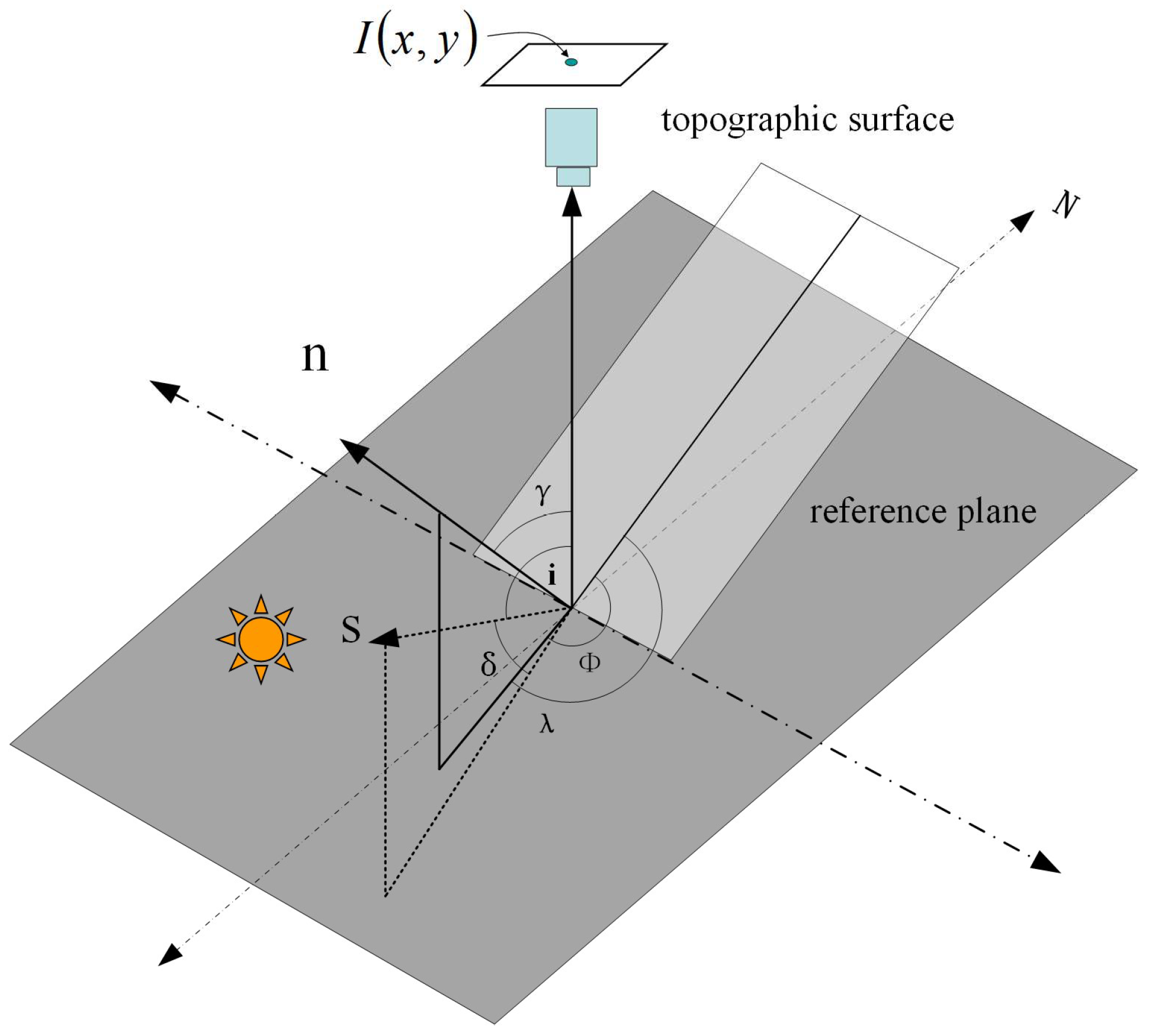
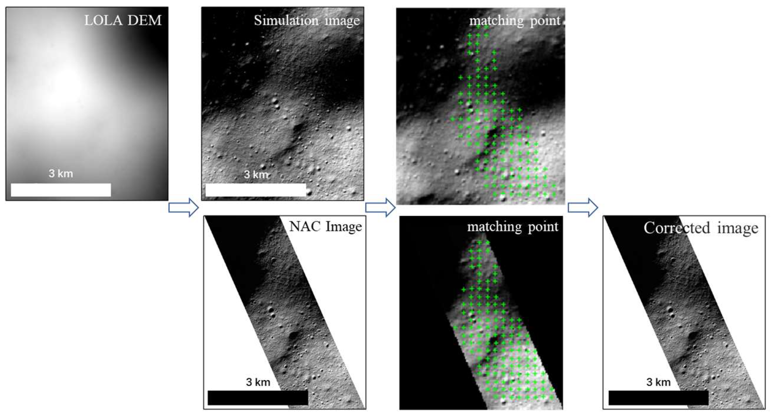
4.1.3. Image Simulation Using DEM

The hill shade technique was employed to generate DEM-simulated illumination images in this research. This method assumes that the lunar surface is an ideal reflector and follows the Lambertian reflectance model. The reflected intensity at a point on the surface depends only on the angle θ i between the direction of sunlight and the surface normal vector (Figure 6).
The slope and aspect can be obtained from a DEM using a third-order inverse distance squared weighting algorithm. The angle θ i between the direction of sunlight and the surface normal vector can be obtained by solving spherical triangles.
I = ρ c o s θ i = ρ n · s = ρ ( cos i cos α + sin i sin α cos ( Φ β ) )
where ρ is the surface albedo, and is assumed to be a constant in this study. s is the direction of solar rays, and n is the direction of surface normal lines.

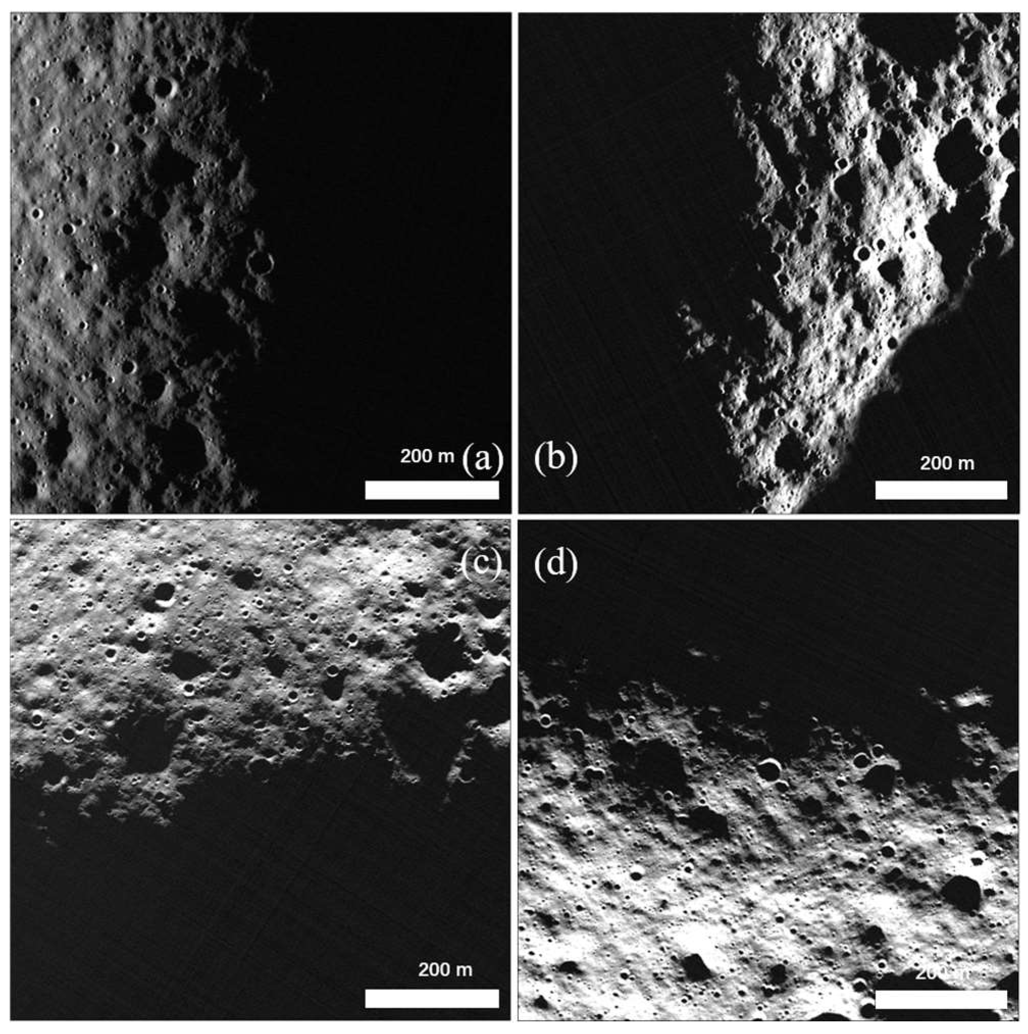
4.2. Illumination Analysis

4.2.1. Illumination Condition Accuracy Assessment

Solar elevation angle and azimuth angle at a specific moment and location for future exploration can be calculated using the ephemeris. The image that closely matches a specific illumination condition in the future can be obtained by querying the nearest solar position from the image dataset. However, affected by various orbital cycles, the images could not fully cover all possible illumination conditions. By analyzing the distribution of azimuth and elevation angles in the dataset, the deviation between the image dataset and the actual illumination conditions is investigated by analyzing the difference in shadows. To quantify the inconsistency in shadow areas, the mismatch rate is used as a measure to analyze the impact of the deviation. The mismatch rate is calculated as follows.
First, images are separately thresholded to obtain their binary matrices, where a value of one represents brightness (sunlit area) and zero represents darkness (shadow area). The threshold is selected to be the 10% of the DN value range in this research. Then, the binary matrix Miss(i, j), which stands for the mismatch of two binary matrices M(i, j) and N(i, j), is obtained using the XOR (Exclusive OR) operation. The total mismatch rate (TMR) is obtained by the ratio of the mismatch region to the total region in the statistical mismatch matrix. N is the total pixel number of the images, and Nmiss is the total number of mismatched pixels.
M i s s ( i , j ) = M ( i , j )     N ( i , j )
T M R = N m i s s   N
In order to distinguish different mismatch types, the ratio between the number of mismatch points and the total pixels in the light zone of the reference image (such as the simulated image) is defined as the light zone mismatch rate (LZMR), and the ratio between the number of mismatch points and the total pixels in the dark zone of the reference image is defined as the dark zone mismatch rate (DZMR) (Figure 7). The dot product of M(i,j) and Miss(i,j) is used to represent the bright mismatch matrix L(i,j), and the dark mismatch matrix D(i,j) is the total mismatch matrix minus the bright mismatch matrix. The TMR, LZMR, and DZMR are used as indices for illumination conditions analysis accuracy.
L ( i , j ) = M ( i , j ) M i s s ( i , j )
D ( i , j ) = M i s s ( i , j ) L ( i , j )
The distribution of shadow variations is presented using a binary map. By comparing the differences between images within the same azimuth range but different elevation angles, as well as images within the same elevation angle range but different azimuth angles, we can select the image with the lowest mismatch rate as the basis of the illumination conditions for a specific moment.

4.2.2. Adaptive Illumination Condition Analysis by Combining Images and DEM

In most cases, images that closely match the required illumination conditions can directly support engineering applications. However, some retrieved nearest sun position images still exhibit significant discrepancies from the actual illumination conditions at certain moments. Combining existing DEM products may improve the accuracy of illumination condition analysis in these situations.
The accuracy of the DEM is the key factor affecting the performance of its illumination condition analysis. As there are no absolute control points and high-precision reference data in the lunar polar region, direct evaluation of DEM accuracy is very challenging. In this paper, we propose a method to evaluate the DEM height errors using mismatched shadow length (MSL) between DEM-simulated image and the actual optical image. By considering the shadow length in the optical image as the ground truth, the mismatched shadow length between the DEM-simulated image and the optical image is statistically calculated in the direction of illumination. This difference in distance between the optical image and the DEM-simulated image in the direction of sunlight is then used to infer height errors based on their geometric relationship. When the actual terrain is higher than the DEM, the shadow length generated by the occlusion of high points (assume that the high point is the measurement base and there is no elevation error) in optical images is shorter than the shadow in the simulated image. Conversely, the shadow length in the optical image is longer than in the simulated image if the actual terrain is lower than the DEM (Figure 8).
Let ∆h be the elevation difference between the DEM data and the actual terrain at the location of the elevation point, with α denoting the solar elevation angle, and ∆d indicating the mismatched shadow length. Based on the geometric relationship depicted in Figure 8, the equation can be derived:
Δ h = Δ dtan α + h B h A  
where h A   and   h B   are elevations of points A and B, respectively, which can be derived from DEM.
The height error calculated by this method is called shadow-based height error (SBHE). Please note that although the formulas used to calculate the mismatch in shadow lengths for dark and bright areas are the same in this method, they reflect different types of height errors. Figure 8a illustrates the case of shadow-mismatch in bright areas of reference, where the shadow length in the actual image is greater than that in the simulated image. The left graph represents the profile view, while the right graph shows the plan view of this situation. The height error location is denoted as point A, which refers to the starting point error, representing the height error at the shadow-mismatch starting position. For the case of shadow-mismatch in dark areas of reference, as shown in Figure 8b, the height error location is denoted as point B, referred to as the endpoint error, representing the height error at the shadow-mismatch endpoint position. The statistical analysis of this error distribution can represent the relative accuracy of the regional DEM in terms of elevation accuracy. This method requires high precision in the matching between simulated and optical images. The datasets obtained through pixel-level registration mentioned earlier are well suited to this method.
By comparing the accuracy of multi-temporal image-based illumination condition analysis with that of DEM-based, we can adaptively select lighting analysis data and methods for engineering support (e.g., task planning) at different locations and different moments.

5. Results and Discussions

5.1. Image Database Construction

As described in Section 2, 226 LROC NAC images and 5 TMC-2 images were selected in this research. These images were preprocessed and orthorectified with ISIS software. Then, the registration of images under different lighting conditions and DEM was performed using the proposed strategy (Figure 9). All images were divided into six groups at 60° azimuth intervals. Six reference images were selected in each group for registration with DEM.
The registration precision between images is high, reaching the sub-meter level, which is higher than the registration precision between the reference image and the DEM. Therefore, the overall accuracy of the dataset depends on the registration precision between the reference image and the DEM (as shown in Table 1). The average precision can reach 2.7 m, achieving the sub-pixel level of the DEM resolution (5 m/pixel).
The solar azimuth and elevation at the time of image acquisition of all the images were calculated. Their distribution is shown in Figure 10.
To cross-verify the results, we calculated the horizon of the center point of the study area using the 5 m/pixel DEM. For the images with the solar position above the horizon, they should appear light, while those below the horizon should appear dark. By manually inspecting the brightness of the central point, we classified 184 images as light and 47 images as dark, which are marked as red and yellow crosses in Figure 10. The image-based results were found to be consistent with the DEM-based results, with only a few small discrepancies. These discrepancies could be attributed to limitations in the DEM accuracy and resolution. These validation results demonstrate the reliability and accuracy of our solar position calculation method, providing support for the subsequent analysis and interpretation of the data.

5.2. Illumination Analysis Results

The multi-temporal image dataset can directly support engineering tasks such as environmental perception. It allows retrieval of the image with the nearest sun position during the task moment. As an example, assuming Chang’E-7 will land on 12 December 2026, at 13:00 UTC, the elevation angle of the landing site is 2.56°, and the azimuth angle is 15.63°. Using the nearest sun position query, the M108252552RE image is obtained with an elevation angle of 2.51° and an azimuth angle of 15.88°. The elevation angle deviation is 1.95%, and the azimuth angle deviation is 1.59%. The lighting conditions are remarkably similar, effectively mirroring the actual illumination scenario. The image’s elevation angle is slightly lower than the actual solar elevation angle, leading to a slightly larger shadow area. Analyzing landing safety based on this image would yield more conservative results, ensuring the security of the landing process.
By utilizing M108252552RE for the extraction of impact craters and shadow areas, a risk distribution map of the landing is generated and shown in Figure 11. Due to the extreme illumination conditions, high-precision automatic extraction of impact craters is still a challenge in the polar region. Here, we manually identified and extracted the impact craters. And we used the threshold segmentation method (see Section 4.2.1 for details) for the shadow extraction. This map can be used to effectively mitigate the risks caused by illumination conditions, providing favorable assurance for the rover exploration of the specific time.

5.2.1. Illumination Condition Accuracy Assessment

From the aforementioned case, it can be seen that the images in the dataset cannot be completely consistent with the actual illumination conditions. In order to evaluate the accuracy of using multi-temporal images for illumination analysis, the distribution of azimuth and elevation angles in the dataset was investigated. Considering that Chang’e-7 plans to conduct a soft landing and surface exploration in 2026, the hourly solar azimuth and elevation angles at the pre-selected landing area were calculated and compared with that of the image dataset. Figure 12a shows the hourly solar elevation and azimuth angles in each month of the year 2026. The images in the dataset were acquired between 2009 and 2012. So, the solar azimuth and elevation angles of these images, which are also shown in Figure 12a, do not exactly match the illumination conditions in 2026. It should be noted that 5 TMC-2 images (represented with yellow crosses in Figure 12a with a resolution of 5 m/pixel are added to the database as supplementary data to increase the coverage of the sun position. There are few LRO images with an azimuth angle of 300°~330° and an elevation angle of 0°~1°. The 5 TMC-2 images can increase the image density in this region. The deviations of the actual solar position from that of the nearest sun position image are then calculated, as shown in Figure 12b. The average deviation of the solar elevation for the nearest sun position image is 0.84°, and the average deviation of the azimuth is 1.27°. The maximum deviation of the solar elevation is 3.16°, and the maximum deviation of the azimuth is 7.78°. Thanks to the acquisition of a large number of overlapping multi-temporal images, this deviation is minimal, but we still need to evaluate its impact on shadow analysis.
The variation in shadow region is related to the solar elevation angle, azimuth angle, and terrain. To separate various influencing factors, three pairs of images with similar azimuth angles but different elevation angles were selected to demonstrate the influence of elevation angle on shadow areas. We selected a test region with consistent terrain and located on the boundary between light and dark areas. The information of the test images is listed in Table 2. The elevation angle intervals for the three pairs of images are 0.9473, 2.1466, and 3.0625, respectively. The image with the lower elevation angle was chosen as the reference image, and the calculated mismatch rates were measured within a 1 km × 1 km area (same for all three pairs). The total mismatch rates are 8.38%, 29.01%, and 18.54%, respectively. The shadow-mismatch map is shown in Figure 13. The results demonstrate a significant impact of elevation angle variation on shadow areas. Additionally, the relationship between the variation in shadow areas and elevation angle is not consistent in different directions. The difference in shadow areas between images with a smaller elevation angle interval may be greater than that between images with a larger elevation angle interval caused by the different azimuth angles of test images.
We also selected three pairs of images with relatively consistent elevation angles but different azimuth angles to demonstrate the influence of solar azimuth angle variations on image shadow areas. The image information is listed in Table 3. The azimuth angle intervals for the three sets of images were 9.45°, 28.60°, and 49.81°, respectively. Taking the image with a smaller azimuth angle variation as the reference image, the mismatch rates were calculated within a 1 km × 1 km area, resulting in total mismatch rates of 11.72%, 18.63%, and 20.73% respectively.
Compared to elevation angle variations, the impact of azimuth angle variations on shadow areas is relatively smaller. Figure 14 illustrates the effects of different azimuth angle variations on shadow areas. The azimuth angle variations exhibit distinct regional characteristics on the mismatch map, with noticeable differences between shadow mismatch and illumination mismatch locations. According to the analysis, when selecting illumination conditions close to the image for illumination analysis, the proximity of the elevation angle should be considered first.

5.2.2. Adaptive Illumination Conditions Analysis

We evaluated the accuracy of illumination condition analysis using the 5 m DEM, as well as the DEM elevation accuracy. Six NAC images of the aforementioned dataset were used to serve as the reference images for shadow-based error detection. The sun azimuth at the time of image acquisition in the test area was calculated, and the corresponding simulated images were rendered with the appropriate illumination conditions. The aforementioned shadow testing method was then used to calculate the mismatch conditions and height errors, obtaining the following nine indicators to assess the quality of lighting simulation and the relative height accuracy of the DEM, TMR, DZMR, LZMR, average MSL (m), maximum MSL, MSL 3σ, average SBHE, maximum SBHE, and SBHE 3σ (three standard deviations). Table 4 presents these indicators, along with the sun azimuth information for the images. The resolution of images ranges from 0.5 to 1 m/pixel and the DEM gird size is 5 m. For convenient comparison, all the data were resampled to 1 m/pixel.
Figure 15 illustrates the mismatched shadow locations and the resulting shadow-based height error. The total mismatched rate ranges from 7.64% to 11.85%, while the mismatched shadow length at 3σ ranges from 20.105 to 24.7064 m, and the mismatch height error at 3σ ranges from 0.7323 to 1.5052 m. The mismatched rate in the bright and dark areas is mainly influenced by the size of the corresponding image regions, leading to significant fluctuations in the results. The overall mismatch rate indicator (TMR) is more robust.
The reliability of using mismatched shadow length to estimate DEM elevation accuracy relies on the number of mismatched shadows as measurements. Images with a sufficient number of shadows were selected as reference images so as to obtain more mismatched shadows for height error estimation. Meanwhile, in order to capture wide and evenly distributed measurements covering the entire area, reference images taken under different illumination conditions were selected. In our experiment, we selected six reference images with different illumination conditions, and obtained a large number of measurements at the same location from different reference images, which we call corresponding measurements. The height errors generated from different reference images should be consistent. We calculated the variance in the shadow-based height error for these corresponding measurements for a consistency check. We conducted 6699 sets of corresponding measurements. The average variance is 0.012 m and the maximum variance is 1.346 m. The frequency distribution result shows that 95% of the variance in the point set is below 0.05 (Figure 16b). This indicates a high level of consistency in the height errors calculated from different reference images under varying illumination conditions, demonstrating the robustness and reliability of this method. Using the height error measurements obtained from all reference images, we interpolated an evaluation accuracy map of the DEM (Figure 16). This can serve as an important reference when using the DEM.
According to the above experimental results, the total mismatch rate of the DEM-simulated images is mostly around 10%. Compared with multi-temporal image-based illumination analysis results, a mismatch rate of 10% approximately corresponds to an elevation angle difference within 1° or an azimuth angle difference within 10°. Therefore, when selecting similar images, using images with an elevation angle difference within 1° or an azimuth angle difference within 10° of a specific moment can yield better results compared to the DEM-simulated images.
The retrieval of the nearest neighboring solar position images in 2026 resulted in a maximum azimuth angle deviation of 7.78°, with all deviations falling within 10°. The average deviation of the elevation angle is 0.84°, with a maximum deviation of 3.16°. Thus, the similarity of the nearest solar position image is mainly influenced by the distribution of elevation angles.
Evaluation angle intervals were interpolated with a 10° azimuth angle range (Figure 17), by which we can assess the azimuth angle deviation between the nearest sun position image and the true situation. For instance, in the 180–270° azimuth interval, the overall deviation is negative, indicating that the image’s elevation angles are generally higher than the true elevation angles. Consequently, the image’s lighting conditions will be better than the true conditions. In intervals with large elevation angle deviations, the DEM-simulated images are better than that of the nearest sun position image for illumination analysis.

6. Conclusions

We proposed a method for lunar polar region illumination condition analyses using multi-temporal high-resolution orbital images. The feasibility of using a nearest solar position image for environmental analysis to support engineering tasks was demonstrated at the study area. Our contributions can be summarized as follows:
(1)
A high-resolution image dataset of a pre-selected landing area of Chang’E-7 was constructed using multi-temporal high-resolution images. And the feasibility of using this dataset for environmental analysis during the mission was demonstrated.
(2)
A registration strategy for multi-temporal overlapping images and DEM was employed to achieve a matching precision of sub-pixel level, effectively eliminating the geometric inconsistencies within the dataset.
(3)
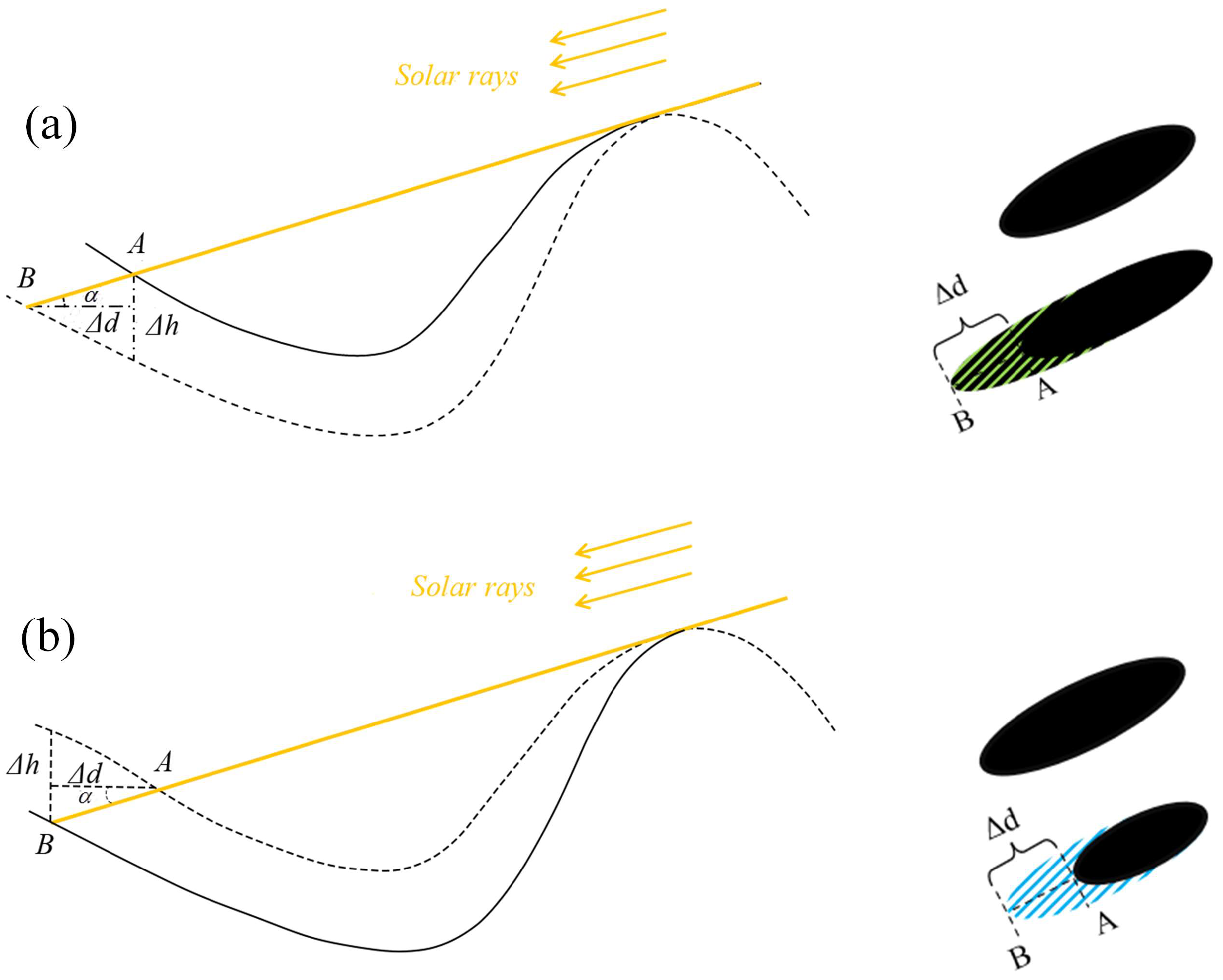
We proposed a mismatch-shadow-length-based approach for an assessment of DEM accuracy, and the precision of illumination condition analysis using a nearest sun position image. The effectiveness and reliability of this method was demonstrated. According to our assessment, an adaptive illumination condition analysis combining images and DEM is proposed.
Due to the different image coverage situations, the effectiveness of the proposed image-based illumination condition analysis varies in different regions. With the continuous acquisition of more high-resolution images, the accuracy of using multi-temporal images for illumination environment analysis will also continue to improve.

Author Contributions

Conceptualization, Y.Z., B.L. and K.D.; Data curation, W.W. and B.X.; Formal analysis, Y.Z., S.L., Z.Y., S.H. and J.W.; Funding acquisition, B.L. and K.D.; Investigation, Y.Z. and B.L.; Methodology, Y.Z. and B.L.; Project administration, B.L. and K.D.; Resources, K.D., S.L., S.H. and J.W.; Software, Y.Z.; Supervision, B.L. and Z.Y.; Validation, S.L., S.H., J.W. and W.W.; Visualization, Y.Z., Z.Y. and B.X.; Writing—original draft, Y.Z. and B.L.; Writing—review and editing, B.L., K.D., S.L. and Z.Y. All authors have read and agreed to the published version of the manuscript.

Funding

This research was supported by the National Key Research and Development Program of China (grant no. 2022YFF0503100) and the Open Fund of the Key Laboratory of Aerospace Flight Dynamics Technology (grant no. KGJ6142210220204).

Data Availability Statement

The LROC NAC images and TMC-2 images are available from the PDS Geosciences Node Lunar Orbital Data Explorer website (https://ode.rsl.wustl.edu/moon/index.aspx) and the Indian Space Science Data Center website (https://pradan.issdc.gov.in/ch2/protected/payload.xhtml) respectively. The improved LDEM is available from https://pgda.gsfc.nasa.gov/products/78. Other datasets generated and analyzed in this study are available from the corresponding author upon reasonable request.

Acknowledgments

We are grateful to the LRO mission team and all those who worked on the Planetary Data System archive for their tireless work in making the LROC images and LDEM publicly available. We thank Barker M.K. and his collaborators for providing the improved LDEM. We are also thankful to the people at the Indian Space Science Data Center for making the TMC-2 images available.

Conflicts of Interest

The authors declare no conflict of interest.

References

  1. Zhang, P.; Dai, W.; Niu, R.; Zhang, G.; Liu, G.; Liu, X.; Bo, Z.; Wang, Z.; Zheng, H.; Liu, C. Overview of the Lunar In Situ Resource Utilization Techniques for Future Lunar Missions. Space Sci. Technol. 2023, 3, 37. [Google Scholar] [CrossRef]
  2. Liu, J.; Zeng, X.; Li, C.; Ren, X.; Yan, W.; Tan, X.; Zhang, X.; Chen, W.; Zuo, W.; Liu, Y.; et al. Landing Site Selection and Overview of China’s Lunar Landing Missions. Space Sci. Rev. 2020, 217, 6. [Google Scholar] [CrossRef]
  3. Li, C.; Wang, C.; Wei, Y.; Lin, Y. China’s present and future lunar exploration program. Science 2019, 365, 238–239. [Google Scholar] [CrossRef]
  4. Smith, M.; Craig, D.; Herrmann, N.; Mahoney, E.; Krezel, J.; McIntyre, N.; Goodliff, K. The artemis program: An overview of nasa’s activities to return humans to the moon. In Proceedings of the 2020 IEEE Aerospace Conference, Big Sky, MT, USA, 7–14 March 2020; pp. 1–10. [Google Scholar]
  5. McKay, C.P. The case for a NASA research base on the Moon. New Space 2013, 1, 162–166. [Google Scholar] [CrossRef]
  6. Carruba, V.; Coradini, A. Lunar cold traps: Effects of double shielding. Icarus 1999, 142, 402–413. [Google Scholar] [CrossRef]
  7. Watson, K.; Murray, B.C.; Brown, H. The behavior of volatiles on the lunar surface. J. Geophys. Res. 1961, 66, 3033–3045. [Google Scholar] [CrossRef]
  8. Qiao, L.; Ling, Z.; Head, J.W.; Ivanov, M.A.; Liu, B. Analyses of Lunar Orbiter Laser Altimeter 1,064-nm Albedo in Permanently Shadowed Regions of Polar Crater Flat Floors: Implications for Surface Water Ice Occurrence and Future In Situ Exploration. Earth Space Sci. 2019, 6, 467–488. [Google Scholar] [CrossRef]
  9. Rao, W.; Fang, Y.; Peng, S.; Zhang, H.; Sheng, L.; Ma, J. Landing Site Selection Method of Lunar South Pole Region. J. Deep Space Explor. 2022, 9, 571–578. [Google Scholar] [CrossRef]
  10. Gläser, P.; Oberst, J.; Neumann, G.A.; Mazarico, E.; Speyerer, E.J.; Robinson, M.S. Illumination conditions at the lunar poles: Implications for future exploration. Planet. Space Sci. 2018, 162, 170–178. [Google Scholar] [CrossRef]
  11. Hu, T.; Yang, Z.; Li, M.; van der Bogert, C.H.; Kang, Z.; Xu, X.; Hiesinger, H. Possible sites for a Chinese International Lunar Research Station in the Lunar South Polar Region. Planet. Space Sci. 2023, 227, 105623. [Google Scholar] [CrossRef]
  12. Wei, G.; Li, X.; Zhang, W.; Tian, Y.; Jiang, S.; Wang, C.; Ma, J. Illumination conditions near the Moon’s south pole: Implication for a concept design of China’s Chang’E−7 lunar polar exploration. Acta Astronaut. 2023, 208, 74–81. [Google Scholar] [CrossRef]
  13. Margot, J.L.; Campbell, D.B.; Jurgens, R.F.; Slade, M. Topography of the lunar poles from radar interferometry: A survey of cold trap locations. Science 1999, 284, 1658–1660. [Google Scholar] [CrossRef]
  14. Vanoutryve, B.; De Rosa, D.; Fisackerly, R.; Houdou, B.; Carpenter, J.; Philippe, C.; Pradier, A.; Jojaghaian, A.; Espinasse, S.; Gardini, B. An analysis of illumination and communication conditions near lunar south pole based on Kaguya Data. In Proceedings of the International Planetary Probe Workshop, Barcelona, Spain, 15 June 2010; pp. 1–7. [Google Scholar]
  15. Bussey, D.; McGovern, J.; Spudis, P.; Neish, C.; Noda, H.; Ishihara, Y.; Sørensen, S.-A. Illumination conditions of the south pole of the Moon derived using Kaguya topography. Icarus 2010, 208, 558–564. [Google Scholar] [CrossRef]
  16. Noda, H.; Araki, H.; Goossens, S.; Ishihara, Y.; Matsumoto, K.; Tazawa, S.; Kawano, N.; Sasaki, S. Illumination conditions at the lunar polar regions by KAGUYA (SELENE) laser altimeter. Geophys. Res. Lett. 2008, 35, 24. [Google Scholar] [CrossRef]
  17. Henriksen, M.; Manheim, M.; Burns, K.; Seymour, P.; Speyerer, E.; Deran, A.; Boyd, A.; Howington-Kraus, E.; Rosiek, M.R.; Archinal, B.A. Extracting accurate and precise topography from LROC narrow angle camera stereo observations. Icarus 2017, 283, 122–137. [Google Scholar] [CrossRef]
  18. Barker, M.; Mazarico, E.; Neumann, G.; Zuber, M.; Haruyama, J.; Smith, D. A new lunar digital elevation model from the Lunar Orbiter Laser Altimeter and SELENE Terrain Camera. Icarus 2016, 273, 346–355. [Google Scholar] [CrossRef]
  19. Mazarico, E.; Neumann, G.; Smith, D.; Zuber, M.; Torrence, M. Illumination conditions of the lunar polar regions using LOLA topography. Icarus 2011, 211, 1066–1081. [Google Scholar] [CrossRef]
  20. De Rosa, D.; Bussey, B.; Cahill, J.T.; Lutz, T.; Crawford, I.A.; Hackwill, T.; van Gasselt, S.; Neukum, G.; Witte, L.; McGovern, A. Characterisation of potential landing sites for the European Space Agency’s Lunar Lander project. Planet. Space Sci. 2012, 74, 224–246. [Google Scholar] [CrossRef]
  21. Gläser, P.; Scholten, F.; De Rosa, D.; Figuera, R.M.; Oberst, J.; Mazarico, E.; Neumann, G.; Robinson, M. Illumination conditions at the lunar south pole using high resolution Digital Terrain Models from LOLA. Icarus 2014, 243, 78–90. [Google Scholar] [CrossRef]
  22. Tong, X.; Huang, Q.; Liu, S.; Xie, H.; Chen, H.; Wang, Y.; Xu, X.; Wang, C.; Jin, Y. A high-precision horizon-based illumination modeling method for the lunar surface using pyramidal LOLA data. Icarus 2023, 390, 115302. [Google Scholar] [CrossRef]
  23. Xin, X.; Liu, B.; Di, K.; Yue, Z.; Gou, S. Geometric quality assessment of chang’E-2 global DEM product. Remote Sens. 2020, 12, 526. [Google Scholar] [CrossRef]
  24. Di, K.; Liu, B.; Xin, X.; Yue, Z.; Ye, L. Advances and applications of lunar photogrammetric mapping using orbital images. Acta Geod. Et Cartogr. Sin. 2019, 48, 13. [Google Scholar]
  25. Barker, M.K.; Mazarico, E.; Neumann, G.A.; Smith, D.E.; Zuber, M.T.; Head, J.W. Improved LOLA elevation maps for south pole landing sites: Error estimates and their impact on illumination conditions. Planet. Space Sci. 2021, 203, 105119. [Google Scholar] [CrossRef]
  26. Wöhler, C.; Grumpe, A.; Berezhnoy, A.; Bhatt, M.U.; Mall, U. Integrated topographic, photometric and spectral analysis of the lunar surface: Application to impact melt flows and ponds. Icarus 2014, 235, 86–122. [Google Scholar] [CrossRef]
  27. Wu, B.; Liu, W.C.; Grumpe, A.; Wöhler, C. Shape and albedo from shading (SAfS) for pixel-level DEM generation from monocular images constrained by low-resolution DEM. Int. Arch. Photogramm. Remote Sens. Spat. Inf. Sci. 2016, 41, 521–527. [Google Scholar] [CrossRef]
  28. Liu, Y.; Wang, Y.; Di, K.; Peng, M.; Wan, W.; Liu, Z. A Generative Adversarial Network for Pixel-Scale Lunar DEM Generation from High-Resolution Monocular Imagery and Low-Resolution DEM. Remote Sens. 2022, 14, 5420. [Google Scholar] [CrossRef]
  29. Tao, Y.; Muller, J.-P.; Conway, S.J.; Xiong, S.; Walter, S.H.G.; Liu, B. Large Area High-Resolution 3D Mapping of the Von Kármán Crater: Landing Site for the Chang’E-4 Lander and Yutu-2 Rover. Remote Sens. 2023, 15, 2643. [Google Scholar] [CrossRef]
  30. Speyerer, E.J.; Robinson, M.S. Persistently illuminated regions at the lunar poles: Ideal sites for future exploration. Icarus 2013, 222, 122–136. [Google Scholar] [CrossRef]
  31. Cisneros, E.; Awumah, A.; Brown, H.; Martin, A.; Paris, K.; Povilaitis, R.; Boyd, A.; Robinson, M. Lunar Reconnaissance Orbiter Camera permanently shadowed region imaging—Atlas and controlled mosaics. In Proceedings of the 48th Annual Lunar and Planetary Science Conference, Houston, TX, USA, 20–24 March 2017; p. 2469. [Google Scholar]
  32. Brown, H.; Boyd, A.; Sonke, A.; Huft, A.; Robinson, M.; Cisneros, E. Lunar Reconnaissance Orbiter Camera Permanently Shadowed Region Images: Updates to PSR Atlas and PSR Mosaics. LPI Contrib. 2022, 2703, 5033. [Google Scholar]
  33. Li, C.; Liu, J.; Ren, X.; Yan, W.; Zuo, W.; Mu, L.; Zhang, H.; Su, Y.; Wen, W.; Tan, X. Lunar global high-precision terrain reconstruction based on Chang’E-2 stereo images. Geomat. Inf. Sci. Wuhan Univ. 2018, 43, 485–495. [Google Scholar] [CrossRef]
  34. Flahaut, J.; Carpenter, J.; Williams, J.-P.; Anand, M.; Crawford, I.; van Westrenen, W.; Füri, E.; Xiao, L.; Zhao, S. Regions of interest (ROI) for future exploration missions to the lunar South Pole. Planet. Space Sci. 2020, 180, 104750. [Google Scholar] [CrossRef]
  35. Liu, N.; Shi, X.; Xu, F.; Jin, Y. Analysis of High Resolution SAR Data and Selection of Landing Sites in the Permanently Shadowed Region on the Moon. Deep. Space Explor. 2022, 9, 42–52. [Google Scholar] [CrossRef]
  36. Robinson, M.S.; Brylow, S.M.; Tschimmel, M.; Humm, D.; Lawrence, S.J.; Thomas, P.C.; Denevi, B.W.; Bowman-Cisneros, E.; Zerr, J.; Ravine, M.A.; et al. Lunar Reconnaissance Orbiter Camera (LROC) Instrument Overview. Space Sci. Rev. 2010, 150, 81–124. [Google Scholar] [CrossRef]
  37. Chowdhury, A.R.; Patel, V.D.; Joshi, S.R.; Arya, A.S.; Ghonia, D.N. Terrain Mapping Camera-2 onboard Chandrayaan-2 Orbiter. Curr. Sci. 2020, 118, 566. [Google Scholar] [CrossRef]
  38. Chowdhury, A.R.; Saxena, M.; Kumar, A.; Joshi, S.; Amitabh, A.D.; Mittal, M.; Kirkire, S.; Desai, J.; Shah, D.; Karelia, J. Orbiter high resolution camera onboard Chandrayaan-2 orbiter. Curr. Sci. 2019, 117, 560. [Google Scholar] [CrossRef]
  39. Smith, D.E.; Zuber, M.T.; Jackson, G.B.; Cavanaugh, J.F.; Neumann, G.A.; Riris, H.; Sun, X.; Zellar, R.S.; Coltharp, C.; Connelly, J. The lunar orbiter laser altimeter investigation on the lunar reconnaissance orbiter mission. Space Sci. Rev. 2010, 150, 209–241. [Google Scholar] [CrossRef]
  40. Becker, K.J.; Anderson, J.A.; Weller, L.A.; Becker, T.L. ISIS support for NASA mission instrument ground data processing systems. In Proceedings of the 44th Annual Lunar and Planetary Science Conference, Woodlands, TX, USA, 18–22 March 2013; p. 2829. [Google Scholar]
  41. Gaddis, L.; Anderson, J.; Becker, K.; Becker, T.; Cook, D.; Edwards, K.; Eliason, E.; Hare, T.; Kieffer, H.; Lee, E. An overview of the integrated software for imaging spectrometers (ISIS). In Proceedings of the Lunar and Planetary Science Conference XXVIII, Houston, TX, USA, 17–21 March 1997; p. 387. [Google Scholar]
  42. Liu, B.; Jia, M.; Di, K.; Oberst, J.; Xu, B.; Wan, W. Geopositioning precision analysis of multiple image triangulation using LROC NAC lunar images. Planet. Space Sci. 2018, 162, 20–30. [Google Scholar] [CrossRef]
  43. Mazarico, E.; Neumann, G.A.; Barker, M.K.; Goossens, S.; Smith, D.E.; Zuber, M.T. Orbit determination of the Lunar Reconnaissance Orbiter: Status after seven years. Planet. Space Sci. 2018, 162, 2–19. [Google Scholar] [CrossRef]
  44. Lowe, D.G. Distinctive image features from scale-invariant keypoints. Int. J. Comput. Vis. 2004, 60, 91–110. [Google Scholar] [CrossRef]
  45. Fischler, M.A.; Bolles, R.C. Random sample consensus: A paradigm for model fitting with applications to image analysis and automated cartography. Commun. ACM 1981, 24, 381–395. [Google Scholar] [CrossRef]
  46. Annex, A.; Pearson, B.; Seignovert, B.; Carcich, B.; Murakami, S.Y. SpiceyPy: A Pythonic Wrapper for the SPICE Toolkit. J. Open Source Softw. 2020, 5, 2050. [Google Scholar] [CrossRef]
  47. Park, R.S.; Folkner, W.M.; Williams, J.G.; Boggs, D.H. The JPL planetary and lunar ephemerides DE440 and DE441. Astron. J. 2021, 161, 105. [Google Scholar] [CrossRef]
  48. Li, X.; Wang, S.; Zheng, Y.; Cheng, A. Estimation of solar illumination on the Moon: A theoretical model. Planet. Space Sci. 2008, 56, 947–950. [Google Scholar] [CrossRef]
Figure 1. Overview of the study area: (a) is shaded relief of LOLA DEM of the south pole of the Moon and 3D display of the study area (the red box area in the left map); (b,c) are the slope and average illumination of the study area, respectively.
Remotesensing 15 05691 g001
Figure 2. Workflow of illumination condition analysis using multi-temporal images.
Remotesensing 15 05691 g002
Figure 3. Example images that need to be removed: (a) is an image (M101436286RE) with lots of bright noise in the shadow area; (b) is an image (M128439353RE) with uneven and inconsistent bright stripe noise.
Remotesensing 15 05691 g003
Figure 4. LROC NAC images with different azimuths: (a) M170255299LE, with azimuth of 267.65°. (b) M189399105RE, with azimuth of 90.21°. (c) M105867878LE, with azimuth of 352.70°. (d) M170771198LE, with azimuth of 194.96°.
Remotesensing 15 05691 g004
Figure 5. Solar azimuth diagram: A is the observation point, B is the sub solar point, O is the Moon’s center of mass, S is the Sun position, and i is the solar incidence angle of the observation point.
Remotesensing 15 05691 g005
Figure 6. Schematic of the factors that influence the intensity of reflectance from the lunar surface. δ and Φ   are the solar elevation angle and azimuth angle at the observation point; γ , λ are slope and aspect, respectively; i is the solar incidence angle.
Remotesensing 15 05691 g006
Figure 7. (a) The binarization map of the DEM-simulated illumination image. (b) The binarization map of NAC image. (c) Shadow-mismatch map using DEM-simulated illumination image as reference (cyan is the consistent area, yellow is the mismatched pixels in the light area, and blue is the mismatched pixels in the dark area. With the TMR is 7.64%, the LZMR is 5.11% and the DZMR is 9.97%).
Remotesensing 15 05691 g007
Figure 8. The figure shows the geometric relationship between the difference in shadow length and the difference in elevation; the right diagram shows the overview diagram of the shadow area change in the corresponding case: (a) The situation where the actual terrain is lower than the DEM terrain. (b) The situation where the actual terrain is higher than the DEM terrain. The solid curve represents the true terrain corresponding to the actual optical image, while the dashed curve represents the DEM data corresponding to the simulated image. The yellow line represents the solar rays. The black ellipse represents the shadow area, and the green line area is shown as light in the real image and with shadow in the DEM-simulated image. The blue line area is shown as shadow in the image and with light in the DEM-simulated image.
Remotesensing 15 05691 g008
Figure 9. Results of registration between DEM and a reference NAC image (M108606146RE). The simulated image is based on LOLA DEM. Green crosses are feature points extracted by SIFT. Image is registered to the LOLA DEM using affine transformation.
Remotesensing 15 05691 g009
Figure 10. The distribution of solar azimuth and elevation. Blue line is the horizon of the center point of the study area (shown in Figure 1). Red and yellow crosses stand for the light and shadow of the center point of the study area in the image, respectively.
Remotesensing 15 05691 g010
Figure 11. Example of environmental perception using the constructed multi-temporal image dataset: (a) M108252552RE with the nearest sun position of demand. (b) Image-based risk distribution map, the red circles represent impact craters, and the blue curves are the shadow boundaries.
Remotesensing 15 05691 g011
Figure 12. Deviation distribution of solar elevation and azimuth angle: (a) Distribution of azimuth and elevation angles in the dataset and the hourly solar positions in 2026. The solar positions for each month are shown in a different color. Red crosses represent the NAC images and yellow crosses represent the TMC-2 images. (b) The difference between hourly solar positions in 2026 and that of the images of the nearest sun positions. (c) Azimuth distribution histogram. (d) Elevation distribution histogram.
Remotesensing 15 05691 g012
Figure 13. The effect of elevation angle on shadow-mismatch: (a,b,d,e,g,h) are the binary maps of M146535043RE, M108252552RE, M126091501LE, M126091501LE, M180056477RE, and M108599352RE, respectively. (c,f,i) are shadow-mismatch maps of the three test groups, respectively, blue and yellow pixels are the shadow-mismatch pixels in the dark and light zone of reference respectively, and cyan represents the area with consistent pixel values.
Remotesensing 15 05691 g013
Figure 14. The effect of azimuth angle on shadow mismatch: (a,b,d,e,g,h) are the binary maps of M1101147258LE, M167914376RE, M184488316LE, M189391940RE, M139444670RE, and M105925266RE, respectively. (c,f,i) are shadow-mismatch maps of the three test groups, respectively, blue and yellow pixels are the shadow-mismatch pixels in the dark and light zone of reference respectively, and cyan represents the area with consistent pixel values.
Remotesensing 15 05691 g014
Figure 15. Shadow-mismatch distribution map (a,c,e,g,i,k) and shadow-based height error map (b,d,f,h,j,l) in test area. The resultant figures are generated from M108585571RE, M110738772RE, M115378448RE, M115701210RE, M1101147258LE, and M1103454419LE, respectively.
Remotesensing 15 05691 g015
Figure 16. (a) Shadow-based height error map of DEM. (b) The variance frequency distribution of the corresponding measurements.
Remotesensing 15 05691 g016
Figure 17. Elevation angle deviation distribution based on 2026 hourly retrieval of the nearest sun position image with 10° azimuth intervals. The triangle is the average, the diamond is the outlier, and the box in the plot represents the interquartile range.
Remotesensing 15 05691 g017
Table 1. Registration precision of reference image and DEM.
Image IDAzimuth (°)Elevation (°)Resolution (m/pixel)Matching Precision RMS (m)
M108211830LE21.72.51.62.8
M112938905RE75.31.61.72.4
M115334726RE98.00.61.72.5
M108606146RE325.92.41.72.7
M105925266RE344.62.01.02.8
M177361050RE345.71.31.43.1
Table 2. The effect of elevation angle on shadow mismatch.
Image IDAzimuth (°)Elevation (°)TMR
(Total Mismatch Rate)
LZMR
(Light Zone Mismatch Rate)
DZMR
(Dark Zone Mismatch Rate)
Group1M146535043RE15.40021.56918.38%9.85%1.80%
M108252552RE15.88582.5164
Group2M126091501LE22.5770−0.419518.54%21.50%0.73%
M110759138RE22.27122.6430
Group3M180056477RE326.28720.281429.01%42.07%0%
M108599352RE326.85272.4280
Table 3. The effect of azimuth angle on shadow mismatch.
Image IDAzimuth (°)Elevation (°)TMR
(Total Mismatch Rate)
LZMR
(Light Zone Mismatch Rate)
DZMR
(Dark Zone Mismatch Rate)
Group4M1101147258LE229.13650.759211.72%6.99%15.15%
M167914376RE238.56570.7575
Group5M184488316LE62.6314−0.982618.63%27.67%11.12%
M189391940RE91.2346−0.9765
Group6M139444670RE294.77010.029320.73%23.89%18.01%
M105925266RE344.58662.0290
Table 4. Accuracy evaluation of illumination conditions analysis using DEM.
Image IDAzimuth (°)Elevation (°)TMRDZMRLZMRAverage MSL(m)Max MSLMSL 3σ(m)Average SBHE (m)Max SBHE(m)SBHE 3σ (m)
M108585571RE2.4396328.80397.64%5.11%9.97%4.34540.962524.70640.17022.79651.4864
M110738772RE2.618925.15319.96%13.54%7.16%4.373740.962524.32380.21232.79061.5052
M115378448RE0.712492.250010.29%30.81%0.03%4.307732.400623.20360.11772.00131.2323
M115701210RE1.503546.29119.10%25.17%2.96%4.407632.575323.36070.09091.26220.7323
M1101147258LE0.7592229.136611.85%12.96%10.46%4.208936.227820.1030.1232.71161.2138
M1103454419LE1.0990263.230510.33%11.96%8.73%4.029930.068923.36070.09472.72561.14
Disclaimer/Publisher’s Note: The statements, opinions and data contained in all publications are solely those of the individual author(s) and contributor(s) and not of MDPI and/or the editor(s). MDPI and/or the editor(s) disclaim responsibility for any injury to people or property resulting from any ideas, methods, instructions or products referred to in the content.

