High-Resolution Mapping of Mangrove Species Height in Fujian Zhangjiangkou National Mangrove Nature Reserve Combined GF-2, GF-3, and UAV-LiDAR

Abstract

Mangroves as an important blue carbon ecosystem have a unique ability to sequester and store large amounts of carbon. The height of mangrove forest is considered to be a critical factor in evaluating carbon sink capacity. However, considering the highly complicated nature of the mangrove system, accurate estimation of mangrove species height is challenging. Gaofen-2 (GF-2) panchromatic and multispectral sensor (PMS), Gaofen-3 (GF-3) SAR images, and unmanned aerial vehicle-light detection and ranging (UAV-LiDAR) data have the capability to capture detailed information about both the horizontal and vertical structures of mangrove forests, which offer a cost-effective and reliable approach to predict mangrove species height. To accurately estimate mangrove species height, this study obtained a variety of characteristic parameters from GF-2 PMS and GF-3 SAR data and utilized the canopy height model (CHM) derived from UAV-LiDAR data as the observed data of mangrove forest height. Based on these parameters and the random forest (RF) regression algorithm, the mangrove species height result had a root-mean-square error (RMSE) of 0.91 m and an R² of 0.71. The Kandelia obovate (KO) exhibited the tallest tree height, reaching a maximum of 9.6 m. The polarization features, HH, VV, and texture feature, mean_1 (calculated based on the mean value of blue band in GF-2 image), had a reasonable correlation with canopy height. Among them, the most significant factor in determining the height of mangrove forest was HH. In areas where it is difficult to conduct field surveys, the results provided an opportunity to update access to acquire forest structural attributes.

1. Introduction

Mangrove forests are plant communities consisting of evergreen trees or shrubs, thriving in the tropical and subtropical inter tidal coasts [1]. They play a crucial role in preventing coastal erosion, maintaining water quality, and preserving biodiversity [2,3,4]. Despite mangrove forests only constituting less than 1% of the total tropical forest area, they remarkably contribute to 11% of the total terrestrial carbon input into the ocean [5,6,7]. However, human activities like deforestation, coastal development, and pollutant discharge have significantly reduced the global mangrove forest area [8,9], endangering their ecological services and carbon storage. Therefore, mapping the spatial distribution of mangrove species and height can furnish a crucial database for the conservation and management of mangrove forests. In addition, accurately and promptly identified tree height provides a key data basis for estimating mangrove forests’ carbon storage and carbon fluxes. However, accurately mapping mangrove forest height presents numerous challenges due to the absence of sensitive image features and the low accuracy of existing retrieval models.

Mangrove forest heights are influenced by complex factors such as tides and community structure [10]. Traditional surveys, while comprehensive, are time-consuming and labor-intensive, making it challenging to meet the demands of real-time, large-scale monitoring [11]. Recently, remote sensing technology has gained popularity as a tool for acquiring tree height information due to its extensive geographical coverage, real-time data acquisition, and multi-angle imaging capabilities. For example, Hyyppä et al. [12] used Spot PAN and Landsat TM data to retrieve forest mean height; Kayitakire et al. [13] assessed the ability of 1 m resolution IKONOS-2 images to estimate the tree height of common spruce. However, these methods often yield low estimation accuracies as optical imagery is not sensitive to the vertical information of trees [14]. The advent and rapid adoption of light detection and ranging (LiDAR) technologies, which provide precise three-dimensional information, have significantly improved the accuracy of tree height capture [15]. Simard et al. [16] produced a global wall-to-wall canopy height map based on the Shuttle Radar Topography Mission (SRTM) 30 m resolution global digital elevation model (DEM), and Geoscience Laser Altimeter System (GLAS) global Lidar altimetry products. A study by Lefsky et al. [17] indicated that stand structure and the mean height and height variability found in LiDAR data are closely associated. However, spaceborne LiDAR data is typically used only for obtaining large-scale tree height information due to its large laser beam width and low laser point density. Furthermore, the high cost of acquiring airborne LiDAR data for the same area is likely one of the biggest obstacles hindering research on large-area tree height extraction. As a result, an increasing number of studies are combining optical images and LiDAR data to accurately map tree heights across large areas. For example, Wang et al. [18] estimated the mangrove forests’ overall height and above-ground biomass (AGB) throughout Hainan Island by combining field sample plots, UAV-LiDAR data and Sentinel-2 image. Zhu et al. [19] combined Landsat-8 images and Multiple Altimeter Beam Experimental Lidar (MABEL) data to create a map of tree height with a 30 m spatial resolution. However, optical images have limitations including saturation problems and the influence of weather conditions, atmosphere, and moisture [20].

With its all-weather, day-and-night operation and penetration capabilities, Synthetic Aperture Radar (SAR) is widely utilized for tree height retrieval [21,22]. Previous studies have demonstrated a strong correlation between tree height and polarization decomposition parameters, as well as radar vegetation indices extracted from polarization SAR [23,24,25]. Furthermore, SAR data can be integrated with optical imagery to capture three-dimensional structural information of forests [26]. Ghosh et al. [27] investigated the potential of Sentinel-2 optical and Sentinel-1 SAR data to develop a novel approach for canopy height estimation in the Bhitarkanika wildlife sanctuary. Existing research primarily integrated Sentinel-2 optical and Sentinel-1 SAR data to construct a feature set for tree height inversion, enabling regional tree height mapping. As the spatial resolution of images is improved, more abundant structural details regarding mangrove forests can be obtained. Compared with the most commonly used Sentinel-1 SAR and Sentinel-2 optical imagery, the high-spatial-resolution Gaofen-3 SAR and Gaofen-2 optical imagery could provide more spectral and structural information for mapping tree height. However, it is not yet clear the capacity of integrating GF-2 Optical and GF-3 SAR for estimating mangrove forest height.

For tree height retrieval, machine learning is a currently widely employed method, with the advantages of low sample consumption and few parameters [28]. In these studies, a common task is use a series of remote sensing observations to develop a predictive model, aiming to predict forest conditions or attributes in unfamiliar scenarios [29]. Among these methods, RF is the most popular and widely used [30]. In a study by Wilkes et al. [31], canopy height was predicted in a 2.9 million ha area of heterogeneous temperate forests by utilizing the RF algorithm, which linked LiDAR-derived canopy height with a combination of satellite imagery (Landsat and MODIS), resulting in an RMSE of 5.68 m. Wang et al. [18] combined field sample plots, UAV-LiDAR data and Sentinel-2 image to retrieve the height of Hainan Island’s mangrove forest using the RF algorithm, resulting in an R² value of 0.67. These studies demonstrated the ability of RF regression model to unveil intricate non-linear connections among variables and the simplicity in tuning the model parameters [30]. Currently, there is a lot of research focused on obtaining forest structure information using RF model [18,19], but there are few studies on mangrove forest height estimation based on GF-2, GF-3, and UAV-LiDAR data. On the other hand, the addition of the mangrove species information could improve the accuracy and stability of the RF regression model in retrieving mangrove forest height.

Based on the above, the purpose of this research is to examine the possibility of using the RF algorithm to estimate the height of mangrove species combining GF-2, GF-3, and UAV-LiDAR data. We extracted characteristic parameters of estimating mangrove species height based on GF-2 and GF-3 imagery. And the CHM derived from UAV-LiDAR data was used as the observed height data of mangrove forest for model training and validation. The specific objectives of this paper include (1) extracting mangrove extent and species information; (2) mining the characteristic parameters related to mangrove species height from GF-2 and GF-3 imagery; (3) mapping the height of the mangrove species by combining UAV-LiDAR, characteristic parameters and RF regression model in the study area; and (4) analyzing the validity parameters used to retrieve the mangrove species height and the spatial characteristics of the mangrove species height in our study area. The results of this study will contribute to a better understanding of mangrove ecosystems and their ecological dynamics, providing basic data for conservation and management efforts. Furthermore, the proposed methodology combining satellite imagery and UAV-LiDAR data with the RF algorithm can serve as a foundation for future research in vegetation height estimation and monitoring in other coastal regions.

2. Materials and Methods

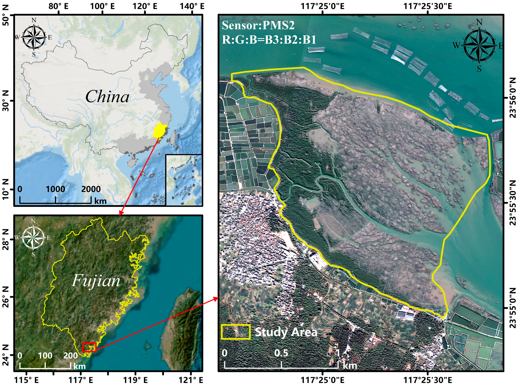
2.1. Study Area

The Fujian Zhangjiangkou National Mangrove Nature Reserve (FZNNR) (117°24′~117°30′E, 23°53′~23°56′N) is situated in the Zhangjiang River Estuary in Yunxiao, Fujian Province, with a total area of 2360 hm². The reserve was established in 1992 and was designated as a National Nature Reserve in 2003. In 2008, it was recognized as a Wetlands of International Importance. The reserve was established in 1992, and in 2003, it received the designation of National Nature Reserve. It was recognized as an Internationally Significant Wetland in 2008. This region boasts the most extensive and thriving natural mangrove community located north of the Tropic of Cancer [32]. The mangroves of FZNNR provides an ideal habitat for more than 150 species of birds, 240 species of aquatic animals, and nearly 400 species of aquatic organisms. The majority of the mangrove forests are concentrated within the core zone of the FZNNR (Figure 1).

FZNNR is a warm humid temperate region with a subtropical maritime monsoon climate. The average yearly temperature is 21.2 °C, and the average yearly precipitation is 1714.5 mm, with the majority of the precipitation falling between April and September. The reserve is generally composed of estuarine waters, intertidal forest wetlands (mangrove swamps), mudflats (intertidal mudflats), and salt marshes, of which the most important type is mangrove forests. Kandelia obovate (KO), Aegiceras corniculatum (AC), and Avicennia marina (AM) are dominant species which account for 55% of the total wetland of FZNNR. Since 2014, Spartina alterniflora (SA) has been expanding explosively in the mudflats at the seaward mudflats. Nowadays, the invasion is still intensifying, Spartina alterniflora is competing with the mangroves at the fringe, and threatening the habitat of local mangroves.

2.2. Data and Pre-Processing

2.2.1. UAV Multi-Spectral Data

The UAV multi-spectral image utilized within the scope of the research was acquired from a DJI Genie 4pro (DJI, Shenzhen, China) equipped with a 1-inch CMOS (Complementary Metal-Oxide-Semiconductor) image sensor. The data were collected on 12 November 2020 when weather was clear and sunny. The collection conditions were low tide period. The flight altitude was set to 200 m, and the course overlap and side overlap were 75% and 80%, respectively. Using Agisoft Metashape-pro 1.8.5 software, we carried out the pre-processing of the UAV image. The processed UAV multi-spectral image has a 0.05 m resolution with the near-infrared band, green band, red band, and blue band, and is used for mangrove extent extraction and species classification.

2.2.2. Gaofen-2 and Gaofen-3 Data

GF-2 PMS image and GF-3 polarimetric SAR data were used to calculate the characteristic indices for the retrieval of mangrove species height. GF-2 is the first civilian optical remote sensing satellite independently developed by China with a revisit period of 5 days. The images include four multispectral bands with 4 m resolution and one panchromatic band with 1 m resolution. The cloud-free GF-2 images were obtained from the website of the China Resources Satellite Application Center (http://www.cresda.com, accessed on 24 June 2023) during low-tide on 25 November 2020. The GF-2 images pre-processing include radiometric calibration, atmospheric correction, geometric correction, and image fusion. Atmospheric correction was carried out using FLAASH atmospheric correction module to remove the effects of atmospheric scattering and absorption. Multispectral bands and panchromatic band were fused using the nearest neighbor diffusion pan-sharpening algorithm. The pre-processing was conducted using the Chinese Domestic Satellite Support Tool in ENVI 5.3.

Developed by the China National Space Administration (CNSA), GF-3 SAR was launched in August 2016 and it is the first Chinese satellite to gather C-band SAR data with multiple polarizations. The spatial resolution of GF-3 data can range from 1 m to 500 m, and the imaging modes cover both single and full polarizations. GF-3 has the most imaging modes (12 imaging modes) covering the traditional strip imaging mode and scanning imaging mode, as well as wave imaging mode for ocean applications and global observation imaging mode. The China Resources Satellite Application Center website (http://www.cresda.com, accessed on 12 April 2023) provided the GF-3 polarimetric SAR data. We acquired two images covering the study area, with level 1A products of SLC (Single-Looking Complex Product) type. One FSI (Fine Striping I) mode image was taken on 29 December 2020, with dual polarization (VV and VH) at 2.6 m spatial resolution. The other FSII (Fine Striping II) mode image was taken on 4 June 2022, with dual polarization (HH and HV) at 4.8 m spatial resolution. The pre-processing was carried out making use of the SARscape module in ENVI 5.6, including data import and generation of SLC files, multi-view processing, filtering, geocoding, and radiometric calibration.

2.2.3. UAV-LiDAR Data

We collected the UAV-LiDAR data on 24 September 2022 during low-tide period by a HS40P sensor mounted on a DJI M600 PRO UAV (DJI, Shenzhen, China). Capable of producing up to 720,000 points per second, the laser sensor operates at a wavelength of 905 nm. In the study area, a total of four flights were conducted at a speed of 6 m/s and an altitude of 100 m. The main processing steps for UAV-LiDAR data include point cloud decomposition, denoising, and ground point classification. Based on base station and POS data, the point cloud decomposition was conducted to calculate accurate geographical positions using LiAcquire 3.3.0 software. The rest of data processing was conducted in LiDAR360 5.3.0 software, including point cloud denoising, and ground and non-ground point classification [33]. At a spatial resolution of 0.5 m, a digital surface model (DSM) and digital elevation model (DEM) were created. UAV-LiDAR data can obtain mangrove forest height with high accuracy [34]. The CHM was produced by deducting the DEM from the DSM. The CHM was used for training and verifying the height prediction model. A total of 340 sample points were randomly selected, and the values of LiDAR-derived height and 47 features were extracted for the training and validation of the height model.

2.2.4. Reference Data

We carried out field surveys in FZNNR from 12 to 15 November 2020. To record the species of mangrove forest and their respective coordinates, a Global Navigation Satellite System (GNSS) equipment was used. Finally, we determined 140 ground points within the scope of the research as a result of the complex growing environment of mangrove forests. According to the field surveys, KO, AC, and AM are the primary mangrove species found in the study area.

2.3. Methods

Figure 2 displays the overall workflow of this study. Firstly, we identified mangrove species based on object-based random forest (OBRF) method and the UAV multi-spectral images. This classification process encompassed multi-scale segmentation, feature extraction, classification, and accuracy assessment. Then, we built a mangrove species height model based on RF regression algorithm and GF-2 images, GF-3 images, and UAV-LiDAR to retrieve the mangrove species height of FZNNR. The retrieval step included feature extraction, model construction, retrieval, and evaluation. Finally, we analyzed the spatial distribution characteristics of mangrove species height and explored the key features for mangrove species height retrieval.

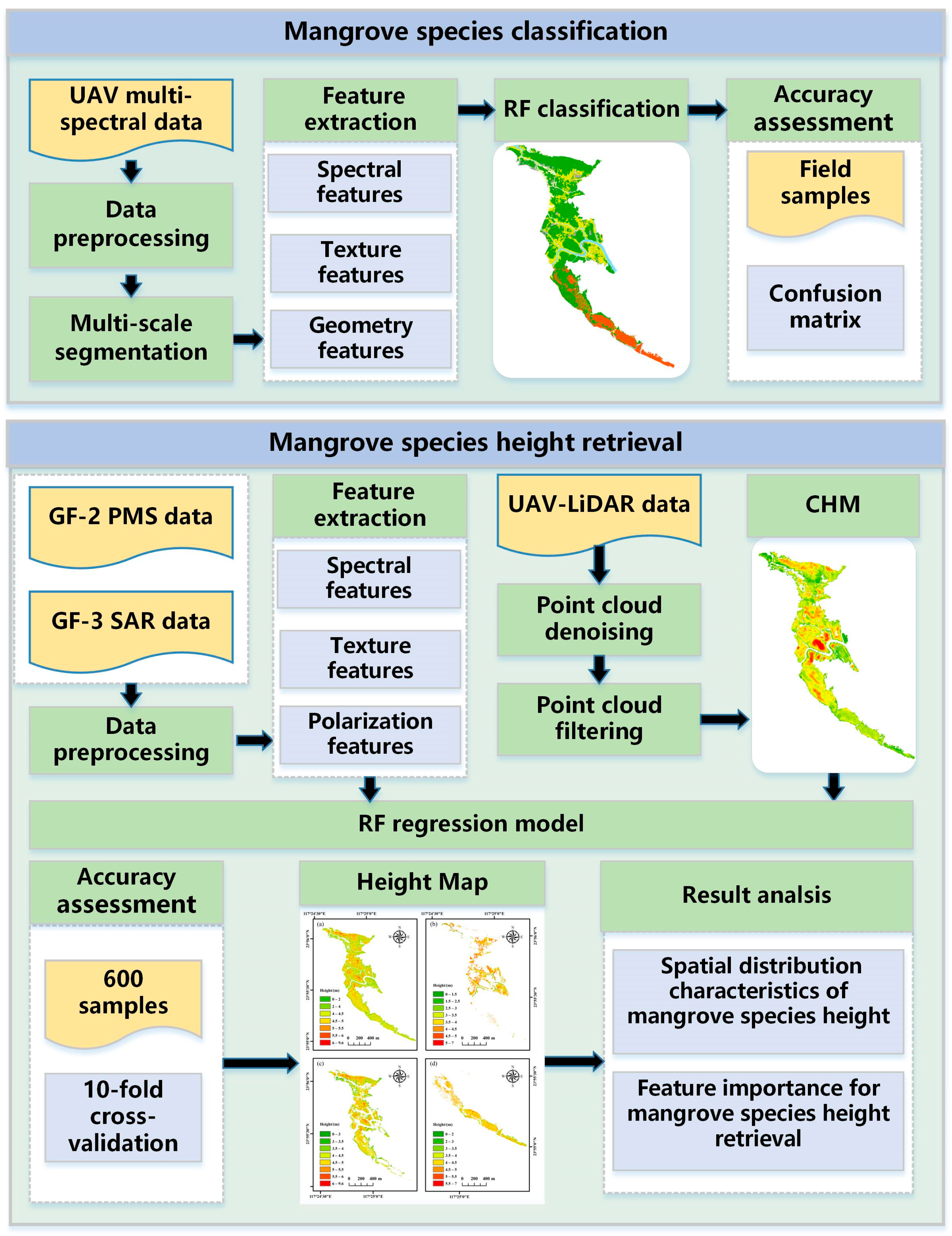
2.3.1. Mangrove Species Classification

To extract mangrove species, we set six landscape types, AC, KO, AM, SA, water, and mudflat, based on the field investigation of landscape types in the study area. In the study, OBRF method was implemented on the Trimble’s eCognition Developer version 9 software to identify mangrove species.

OBRF classification method takes the image object as the fundamental unit of analysis, incorporating spectral features, texture, shape, and contextual information to distinguish landscape types. In this method, multi-scale segmentation was used to establish a hierarchical network structure of image objects, including the shape, compactness, and shape parameters [35]. The scale parameter is the determining parameter for the segmentation effect. The optimal scale parameter depends on the sensor type, resolution, segmentation objectives, and target objects. In this study, the optimal scale parameter for mangrove species classification was determined by visual experience based on the principle of “homogeneity” of the spectral and spatial. Finally, the shape value, compactness value and scale value were set to 0.2, 0.8, and 75, respectively.

We extracted the spectral reflectance, spectral indices, and texture information as the classification features based on UAV multi-spectral images. The specific classification features included mean and standard deviation of the four spectral bands (blue, green, red, and NIR), six spectral indices (NDVI, DVI, FDI, Cig, EVI, and SR), two geometry indices, and seven texture indices (

Table 1. The formulas of the 47 features for mangrove species height retrieval.

Features			Formula
Features based on GF-2	Spectral bands	B1, B2, B3, B4	-
	Vegetation indices	Cig [36]	(B4/B2) – 1
		DVI [37]	B4 – B3
		EVI [38]	$\frac{2.5\times (\mathrm{B}4-\mathrm{B}3)}{\mathrm{B}4+6\times \mathrm{B}3-7.5\times \mathrm{B}1+1}$
		FDI [39]	B4 – (B2 + B3)
		NDVI [40]	(B4 – B3)/(B4 + B3)
		SR [41]	B4/B3
		TNDVI [42]	$\sqrt{0.5+\frac{\mathrm{B}4-\mathrm{B}3}{\mathrm{B}4+\mathrm{B}3}}$
	Texture features	Mean [43]	$\frac{1}{MN}{\displaystyle \sum _{i=0}^{M-1}}{\displaystyle \sum _{j=0}^{N-1}}f(i,j,d,\theta )$
		Variance [43]	${\displaystyle \sum _{i=0}^{M-1}}{\displaystyle \sum _{j=0}^{N-1}}{\left(i-\mu \right)}^{2}f(i,j,d,\theta )$
		Homogeneity [43]	${\displaystyle \sum _{i=0}^{M-1}}{\displaystyle \sum _{j=0}^{N-1}}\frac{f(i,j,d,\theta )}{1+{(i-j)}^2}$
		Contrast [43]	${\displaystyle \sum _{i=0}^{M-1}}{\displaystyle \sum _{j=0}^{N-1}}{\left(i-j\right)}^{2}f(i,j,d,\theta )$
		Dissimilarity [43]	${\displaystyle \sum _{i=0}^{M-1}}{\displaystyle \sum _{j=0}^{N-1}}\left|i-j\right|f(i,j,d,\theta )$
		Entropy [43]	$-{\displaystyle \sum _{i=0}^{M-1}}{\displaystyle \sum _{j=0}^{N-1}}f(i,j)lgf(i,j,d,\theta )$
		Second Moment [43]	${\displaystyle \sum _{i=0}^{M-1}}{\displaystyle \sum _{j=0}^{N-1}}{f(i,j,d,\theta )}^2$
		Correlation [43]	${\displaystyle \sum _{i=0}^{M-1}}{\displaystyle \sum _{j=0}^{N-1}}\frac{(i-\mu )(j-\mu ){f(i,j,d,\theta )}^2}{{\delta }^2}$
Features based on GF-3	Polarization parameters	HH	-
		HV	-
		VV	-
		VH	-

). Then, the RF algorithm was applied to classify mangrove species based on the homogeneous image objects. RF algorithm can handle high and non-normal distribution data, and can integrate image data sources of different dimensions with auxiliary data into the workflow of image classification, which is a mature machine classification model at present. Ntree and mtry are two important parameters that affect the accuracy and operational efficiency of RF model. The variables ntree and mtry indicate the number of decision trees needed to construct the RF model and the maximum number of features randomly selected from the dataset for split decisions made during each decision tree creation, respectively. In this RF model, we set mtry and ntree to 5 and 500, respectively.

2.3.2. Mangrove Species Height Retrieval

To estimate the mangrove species height within the FZNNR, we extracted 47 features from GF-2 and GF-3 data for building the height model. Based on GF-2, we extracted four band reflectance features (blue, green, red, and NIR), seven vegetation index features (CIg, DVI, EVI, FDI, NDVI, SR, TNDVI), and 32 texture features (Mean, Variance, Homogeneity, Contrast, Dissimilarity, Entropy, Second Moment, and Correlation for each single band). Based on GF-3 SAR image, we obtained four polarization features (HH, HV, VV, and VH). The 47 features are shown in Table 1.

2.3.3. Random Forest Regression Model

The height of mangrove species in FZNNR was estimated using the RF regression algorithm. The RF regression algorithm is a nonparametric statistical estimation method that explores the complex nonlinear relationships between dependent variables and predictor variables [44]. The basic theory of RF regression model is the building of numerous decision trees [45], and subsequently calculating the final predicted value by averaging the predicted values of all trees [46]. Usually, the algorithm randomly selects 2/3 of the original sample to build the decision tree, and the remaining 1/3 of the data is used as out-of-bag data (OOB) to validate the decision tree.

Large amounts of features can affect the accuracy of RF models. Therefore, it is one of the most important steps to filter out the effective features for building mangrove species model [47]. In this study, we use SHapley Additive exPlanations (SHAP) value to evaluate and filter feature variables. SHAP is a methodology employed to elucidate the contribution of features in model predictions. It employs the concept of Shapley Value from game theory to determine the contribution value of each feature in model prediction. It incorporates existing machine learning algorithms, like neural networks and RF, and calculates all possible feature combinations in the model to accurately obtain relative importance information for each feature [48]. The computation method of SHAP value surpasses other indicators like Gini importance and information entropy by considering all combinations of features, which provided a more precise assessment of highly correlated features and nonlinear combination features [49].

2.3.4. Accuracy Assessment

For accuracy assessment of the mangrove species classification result, we calculated the overall accuracy (OA), the producer’s accuracy (PA), the user’s accuracy (UA), and Kappa coefficient based on the confusion matrix (the rows of the matrix represent ground truth classes and the columns of the matrix represent predicted classes). The equations are as follows:

$$OA={\sum }_{i=1}^n\raisebox{1ex}{$P_{ii}$}\!\left/ \!\raisebox{-1ex}{$P$}\right.$$

(1)

$${PA}_i=\raisebox{1ex}{$P_{ii}$}\!\left/ \!\raisebox{-1ex}{$P_{i+}$}\right.$$

(2)

$${UA}_i=\raisebox{1ex}{$P_{ii}$}\!\left/ \!\raisebox{-1ex}{$P_{+i}$}\right.$$

(3)

$$Kappa=\frac{P{\sum }_{i=1}^n{P}_{ii}-{\sum }_{i=1}^n\left({P_i}_{+}{P_{+}}_i\right)}{P^2-{\sum }_{i=1}^n\left(P_{i+}{P}_{+i}\right)}$$

(4)

In the above categories, $p$ represents the sum of samples, $P_{ii}$ represents the number of samples in row $i$ and column $i$ of the error matrix, ${P_{+}}_i$ represents the sum of class $i$ in the classification results, ${P_i}_{+}$ represents the sum of class $i$ in the ground reality data, and $n$ represents the number of categories.

For accuracy assessment of the mangrove species height result and the ability of the model, we used the 10-fold cross-validation method. The 10-fold cross-validation divides the dataset equally (or approximately) into 10 subsets, uses nine of them to build the model, and leaves one as the validation set. The coefficient of determination (R²) and root-mean-square-error (RMSE) between the predicted mangrove specie height and the CHM data were calculated to evaluate the accuracy of the model. The equations are as follows:

$$R^2=1-\frac{{(y_i-{\widehat{y}}_i)}^2}{{(y_i-\overline{y})}^2}$$

(5)

$$RMSE=\sqrt{\frac{\sum _{i=1}^n{(y_i-{\widehat{y}}_i)}^2}{n}}$$

(6)

where $n$ is the number of samples, $y_i$ and ${\widehat{y}}_i$ represent the true and predicted values of mangrove specie height at sample point $i$, respectively, and $\overline{y}$ represents the average of the true values of tree height.

3. Results

3.1. Accuracy Assessment

The result of accuracy assessment of the mangrove species classification is displayed in

Table 2. The confusion matrix of the mangrove community classification results.

Community Type	Validation Samples							UA (%)
	KO	AC	AM	SA	Mudflat	Water	Total
KO	36	2	1	0	0	0	39	92.31
AC	0	28	1	0	0	0	29	96.55
AM	2	1	24	1	0	0	28	85.71
SA	0	0	1	20	0	0	21	95.24
Mudflat	0	0	0	1	10	1	12	83.33
water	0	0	0	0	1	10	11	90.91
Total	38	31	27	22	11	11	140
PA (%)	94.74	90.32	88.89	90.91	90.91	90.91	94.74
Kappa: 0.89		OA: 91.43%

. The OA of the mangrove species result was 91.43% (kappa = 0.89). KO reached the highest producer’s accuracy (94.74%), followed by AC with 90.32% and AM with 88.89%. The error was mainly due to the misclassification between KO, AC, and AM at the center of the research area and the misclassification between AM and SA.

We randomly selected 600 sample points based on the CHM derived from the LiDAR data to evaluate the mangrove species height model constructed by RF regression method. The RMSE of the result was 0.91 m, and R² was 0.71. Figure 3 shows the accuracy assessment of the mangrove species height result.

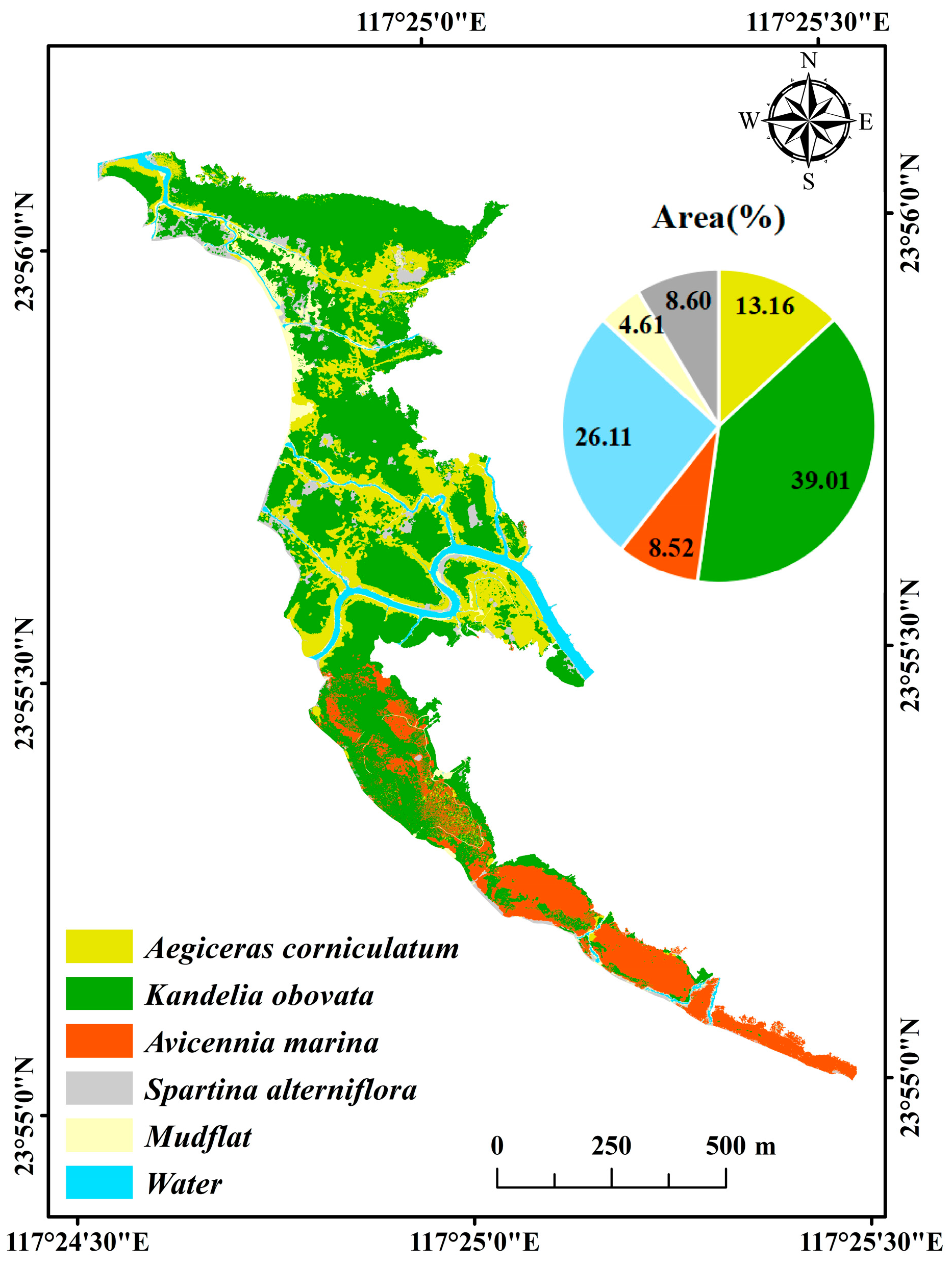
3.2. The Distribution of Mangrove Species of FZNNR

The distribution of mangrove species in FZNNR is shown in Figure 4, which was obtained based on the UAV multi-spectral image and OBRF method. The total area of mangrove forest in FZNNR was 50.92 ha. KO was the dominant mangrove species in FZNNR, with a total area of 32.73 ha. The total area of AC was 11.04 ha, mainly distributed on both sides of the water; and the total area of AM was 7.15 ha, mainly distributed in the central and southern part of the study area.

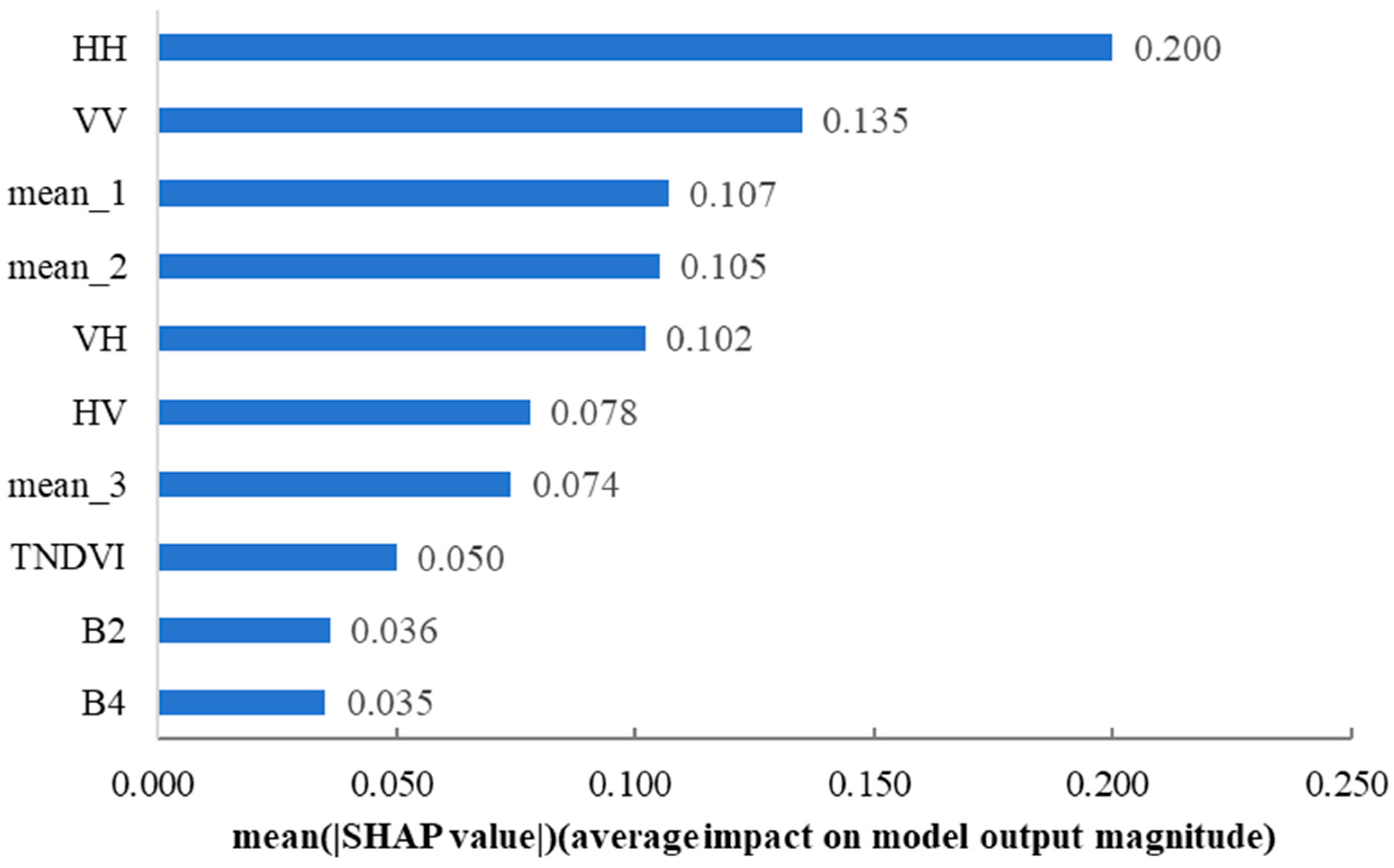
3.3. Feature Importance for Mangrove Species Height Retrieval

In this study, the 47 features extracted from GF-2 PMS and GF-3 SAR images were filtered using the SHAP value in machine learning, and the results are presented in Figure 5. The RF model picked ten features for the purpose of estimating the height of mangrove species. Of these ten characteristics, the most important feature was the backward scattering coefficients of HH polarization from GF-3 SAR images, followed by VV polarization feature and the texture features of mean_1 (Calculated based on the blue band) from GF-2 images. The results indicated that the backscattering coefficient features of GF-3 images and the texture features of GF-2 images are the effective features for the mangrove species height estimation.

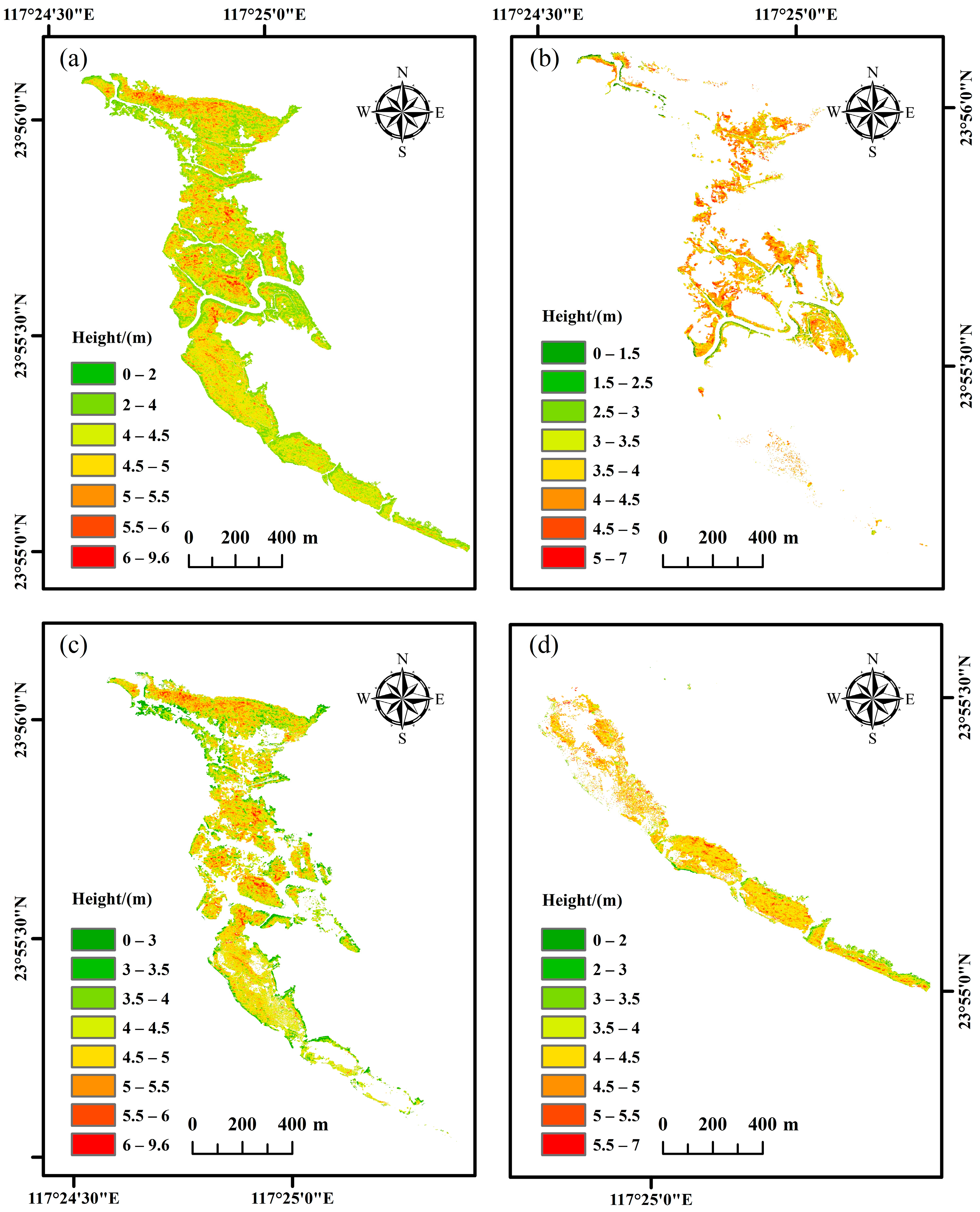
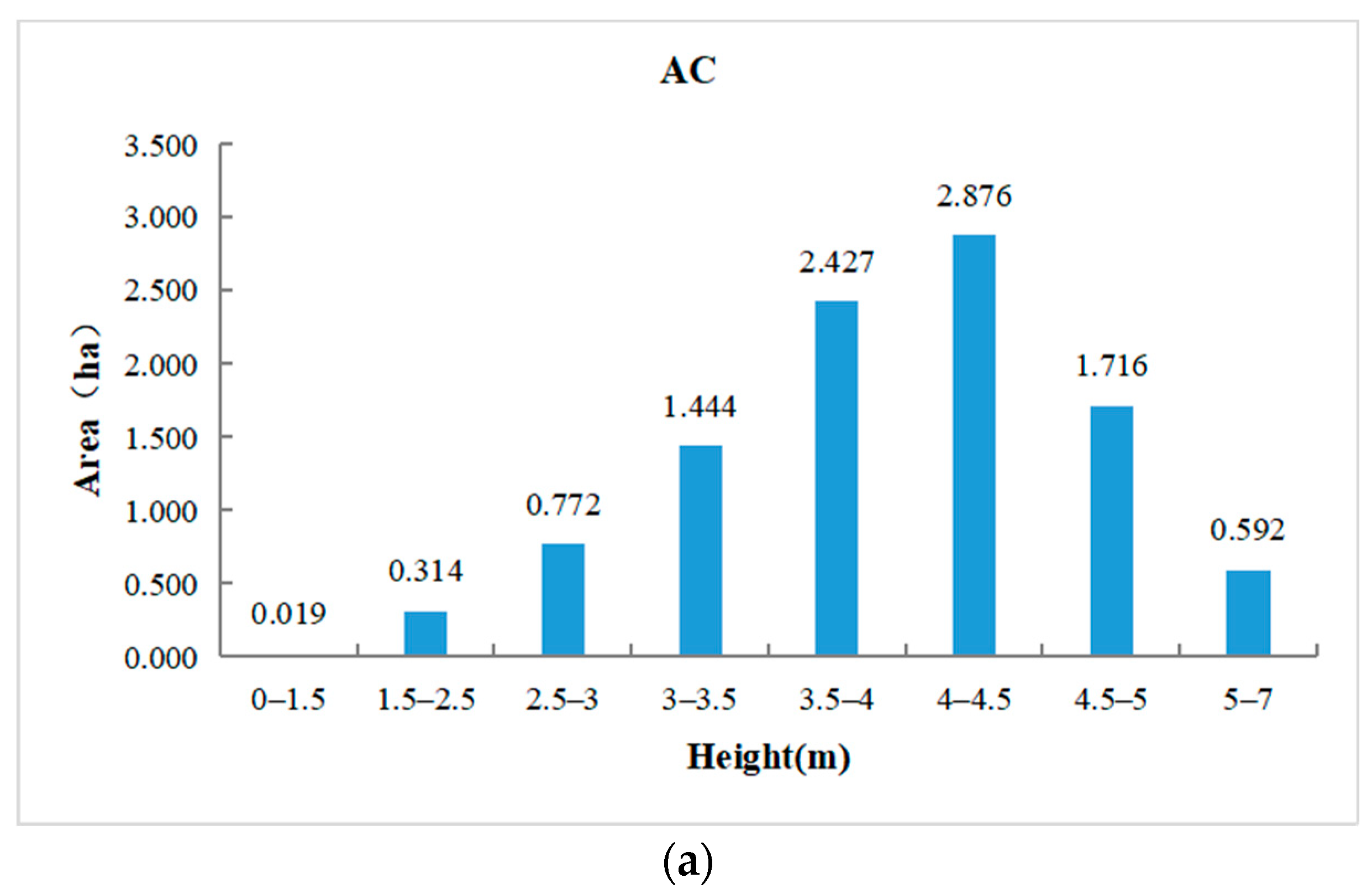
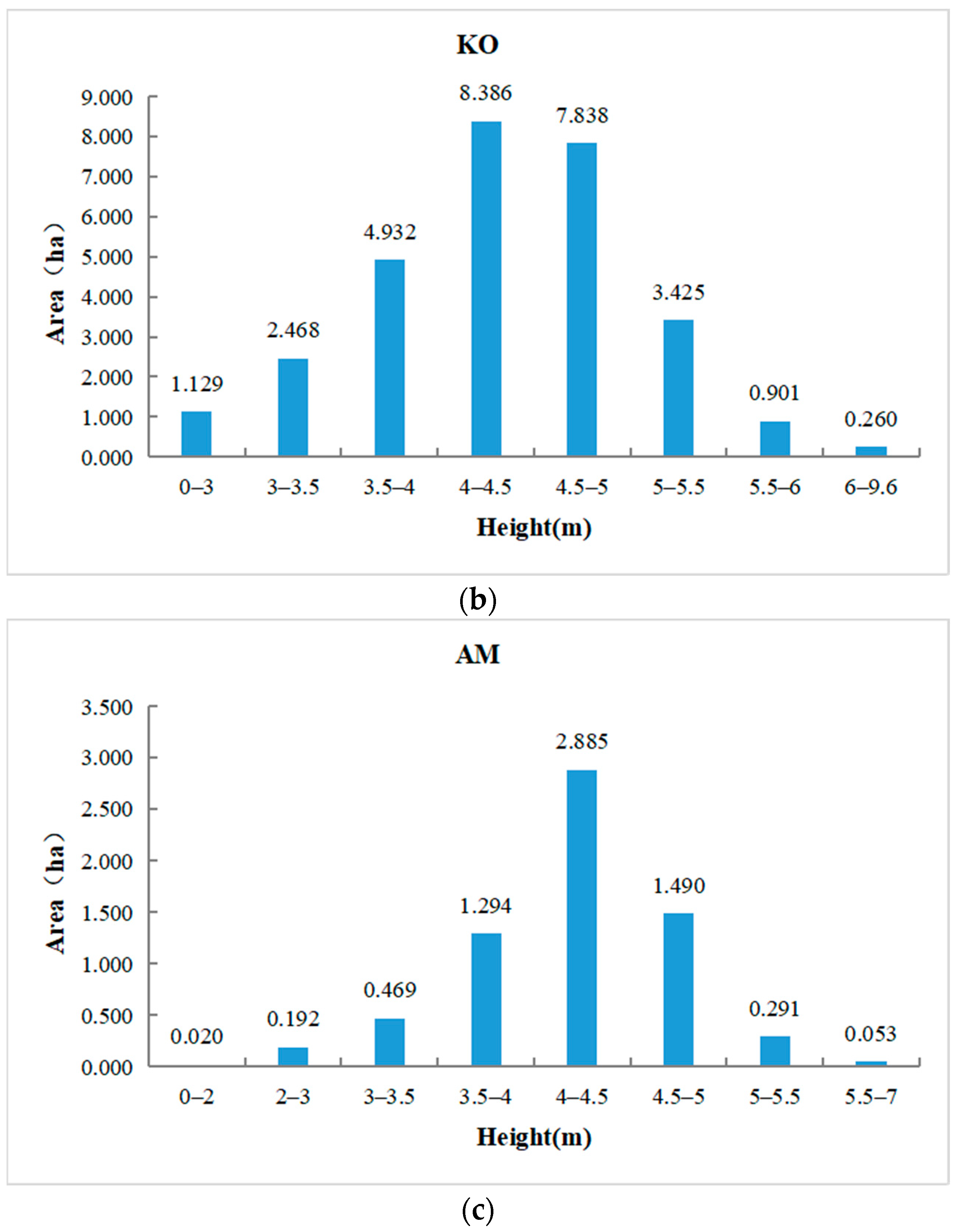
3.4. The Spatial Distribution of Mangrove Species Height in FZNNR

To retrieve the mangrove species height in FZNNR (Figure 6), we used the RF regression model based on the UAV-LiDAR, GF-2, and GF-3 images. Our findings suggested that mangrove forests varied in height from 0.4 to 9.6 m (Figure 7). Heights exceeding 5.5 m were primarily found in the central zone of the study area, while heights less than 2 m were observed at the edges of the study area. The distribution map indicated that the height ranges for AC, KO, and AM were, respectively, between 4 and 7 m. The height map of the mangrove species, presented at a resolution of 0.8 m, is shown in Figure 6. For the species AC, the largest area (2.876 ha) is observed in the height interval of 4 m to 4.5 m. The second and third largest areas are found in the intervals of 3.5 m to 4 m (2.427 ha) and 4.5 m to 5 m (1.716 ha), respectively. In the case of KO, the largest area is within the 4 m to 4.5 m range, covering approximately 8.386 ha. The next largest areas are within the ranges of 4.5 m to 5 m (7.838 ha) and 3.5 m to 4 m (4.932 ha). For AM, the largest area (2.885 ha) is within the 4 m-to-4.5 m height interval, followed by the intervals of 4.5 m to 5 m (1.490 ha) and 3.5 m to 4 m (1.294 ha).

4. Discussion

In our research, we combined UAV-LiDAR data, GF-2 Optical, and GF-3 SAR images to map the height of mangrove species at a resolution of 0.8 m in FZNNR, utilizing an RF regression model. We extracted a total of 47 feature variables and selected the 10 most relevant features which have a strong correlation with the height of mangrove species. These 10 selected features were used to construct the prediction model for mangrove forest height retrieval. The results demonstrated that these selected features effectively predict the height of the mangrove forest. Furthermore, the results validated the exceptional effectiveness of GF-3 SAR and GF-2 PMS in estimating the height of the mangrove species.

4.1. Feature Variable Importance

In this study, the machine learning SHAP value was utilized to filter the 47 features that were extracted from GF-2 PMS and GF-3 SAR data. The SHAP value calculates the contribution of each feature to the model output, considering the interactions between features [50]. Consequently, it provides a more precise depiction of feature impact on predicted outcomes, particularly for nonlinear models, surpassing other methods (such as feature importance) in terms of accuracy. Therefore, we choose the SHAP value to evaluate the importance of 47 features in RF model. Finally, ten features were selected by the SHAP value in order to estimate mangrove species height. The analysis of feature importance revealed that the HH of GF-3 SAR data was pivotal in predicting mangrove species height, followed by the VV of GF-3 SAR data. SAR imagery can emit radiation to identify and measure branches and trunks in order to determine the structure of the canopy [51]. This finding aligns with Liu et al., who affirmed the efficacy of backscattering variables (VV, VH) from Sentinel-1B images in estimating the mean height of forest stands at a 10 m resolution [20]. Zhu et al. [52] estimated the AGB of mangrove plantations by integrating fixed-wing UAV-based DSM, GF-2 optical, and GF-3 SAR data. They found that HH and HV played significant roles in AGB prediction. The texture features of mean_1 and mean_2 was ranked third and fourth in importance, respectively. These features represent the mean of the texture indices calculated by the blue and red bands of GF-2. This observation mirrors Kayitakire et al., who also discovered that texture indices extracted from IKONOS-2 were effective in inverting forest structure parameters [13]. Similarly, Sarker and Nichol [53] confirmed that texture indices of ALOS AVNIR-2 can enhance their estimation accuracy of forest biomass. Texture indices from high-resolution remote sensing images augment the discrimination of spatial information based on the original brightness of images, thereby playing a crucial role in inverting forest structure parameters.

4.2. Accuracy of Random Forest Regression Model

This study set out to construct a robust and precise model for estimating the height of mangrove species. In order to build non-linear connections between the height and features, we utilized an RF regression model, owing to its resilience to outliers in the training data, capability to handle non-parametric data, ability to reveal complex non-linear relationships between variables, and ease of model parameter tuning.

Previous studies have utilized machine learning algorithms such as stepwise multiple regression and multiple regression for forest height estimation. For instance, Zhu et al. [19] developed forest height models using both RF and stepwise multiple regression algorithms. Their findings revealed that estimates of forest height produced by the stepwise multiple regression model were less accurate than those generated by the RF model. Similarly, for the purpose of estimating forest properties, Luther et al. [54] used multiple regression and RF models, with the RF model outperforming the multiple regression model. These studies collectively demonstrated that the RF algorithm provides more accurate regression prediction results than other machine learning algorithms.

In our study, we constructed an RF model to estimate mangrove species height, achieving a good performance (R² = 0.71, RMSE = 0.91 m). Compared with previous studies on tree height prediction, our study demonstrated some improvement in prediction accuracy. For example, Simard et al. [55] successfully estimated mean tree height and biomass in mangrove forests in the Everglades National Park using Shuttle Radar Topography Mission (SRTM) elevation data, with an RMSE of 2.0 m for mean mangrove height estimation. Our study improved upon this precision, potentially due to the high spatial resolution of the data we used. Wang et al. [18], who retrieved the height of Hainan Island’s mangrove forest using Sentinel-2 imagery, achieved an RMSE of 1.90 m and an R² of 0.67—a lower R² than that in our study and a higher RMSE. This could be because Sentinel-2 images have a lower spatial resolution than GF-2 images. The higher RMSE in Wang’s study could be caused by the reality that the average height of mangroves in Hainan Island is greater than that in Zhangjiang Estuary. Overall, our model achieved a good performance (R² = 0.71, RMSE = 0.91 m), demonstrating that the RF algorithm holds significant potential for estimating mangrove forest height.

4.3. Limitations and Potentials

In our study, the RF regression model for estimating mangrove species height was influenced by raster matching issues between multiple data sources (GF-2, GF-3). The collection time of various data sources also had an impact on model accuracy, but this was within the error range, given the slow growth and relatively stable height of mangrove forests over several years.

The inherent limitations of GF-2 optical data may have contributed to the discrepancy between predicted height and the CHM. Despite its high spatial resolution, GF-2 image only has four bands and lacks the red-edge band and short-wave infrared band, which are sensitive to mangrove growth. Active sensors such as SAR and UAV-LiDAR could have mitigated this problem. The GF-3 SAR data used in this study address this limitation to mangrove species height prediction.

The RF algorithm can effectively handle high-dimensional and nonlinear regression problems, demonstrating high generalization ability and stability. However, it has some limitations. The RF model assumes a normal or approximate normal distribution of the data due to its reliance on the Mean Squared Error (MSE) as the loss function. This assumption could lead to large bias and variance in the model if not met [56]. Moreover, the RF model is sensitive to noise data and outliers, which may affect its accuracy and stability [57,58]. In addition to the limitations of the RF model, only spectral features, texture features, and SAR features were considered in this study, and other factors such as species and climate were not considered.

5. Conclusions

Combining GF-2, GF-3, and UAV-LiDAR data, our research investigated the possibility of estimating mangrove species height in FZZNR. We constructed a height retrieval model by integrating both GF-2 and GF-3 imagery with the CHM derived from UAV-LiDAR, based on the RF regression algorithm. The suggested the height retrieval model had an R² of 0.71 and an RMSE of 0.91 m, indicating good performance. Of the all features, the texture features and SAR features were crucial in mangrove height estimations. This method can overcome the accuracy limitations of a single remote sensing data source and improve the accuracy and reliability of mangrove forest height estimation. This study also demonstrated the advantage of using the CHM derived from UAV-LiDAR as the training data, which can reduce the cost and time of field measurements. Our study provided an effective technical means for further monitoring and managing mangrove ecosystems using multi-source remote sensing data. In future studies, we will explore the potential of using other remote sensing data, such as hyperspectral data, for mapping mangrove forest height and explore the ability of GF-2 and GF-3 data for mapping other structural information.

References

1. Zhang, Z.; Pan, J.; Pan, Y.; Li, M. Biogeography, assembly patterns, driving factors, and interactions of archaeal community in mangrove sediments. Msystems 2021, 6, e01381-20. [Google Scholar] [CrossRef] [PubMed]
2. Wang, L.; Jia, M.; Yin, D.; Tian, J. A review of remote sensing for mangrove forests: 1956–2018. Remote Sens. Environ. 2019, 231, 111223. [Google Scholar] [CrossRef]
3. Wu, L.; Wang, L.; Shi, C.; Yin, D. Detecting mangrove photosynthesis with solar-induced chlorophyll fluorescence. Int. J. Remote Sens. 2022, 43, 1037–1053. [Google Scholar] [CrossRef]
4. Zeng, H.; Jia, M.; Zhang, R.; Wang, Z.; Mao, D.; Ren, C.; Zhao, C. Monitoring the light pollution changes of China’s mangrove forests from 1992-2020 using nighttime light data. Front. Mar. Sci. 2023, 10, 1187702. [Google Scholar] [CrossRef]
5. Donato, D.C.; Kauffman, J.B.; Murdiyarso, D.; Kurnianto, S.; Stidham, M.; Kanninen, M. Mangroves among the most carbon-rich forests in the tropics. Nat. Geosci. 2011, 4, 293–297. [Google Scholar] [CrossRef]
6. Friesen, S.D.; Dunn, C.; Freeman, C. Decomposition as a regulator of carbon accretion in mangroves: A review. Ecol. Eng. 2018, 114, 173–178. [Google Scholar] [CrossRef]
7. Giri, C.; Ochieng, E.; Tieszen, L.L.; Zhu, Z.; Singh, A.; Loveland, T.; Masek, J.; Duke, N. Status and distribution of mangrove forests of the world using earth observation satellite data. Glob. Ecol. Biogeogr. 2011, 20, 154–159. [Google Scholar] [CrossRef]
8. Jia, M.; Wang, Z.; Mao, D.; Ren, C.; Song, K.; Zhao, C.; Wang, C.; Xiao, X.; Wang, Y. Mapping global distribution of mangrove forests at 10-m resolution. Sci. Bull. 2023, 68, 1306–1316. [Google Scholar] [CrossRef]
9. Wu, W.; Zhi, C.; Gao, Y.; Chen, C.; Chen, Z.; Su, H.; Lu, W.; Tian, B. Increasing fragmentation and squeezing of coastal wetlands: Status, drivers, and sustainable protection from the perspective of remote sensing. Sci. Total Environ. 2022, 811, 152339. [Google Scholar] [CrossRef]
10. Bathmann, J.; Peters, R.; Reef, R.; Berger, U.; Walther, M.; Lovelock, C.E. Modelling mangrove forest structure and species composition over tidal inundation gradients: The feedback between plant water use and porewater salinity in an arid mangrove ecosystem. Agric. For. Meteorol. 2021, 308, 108547. [Google Scholar] [CrossRef]
11. Hadadi, F.; Moazenzadeh, R.; Mohammadi, B. Estimation of actual evapotranspiration: A novel hybrid method based on remote sensing and artificial intelligence. J. Hydrol. 2022, 609, 127774. [Google Scholar] [CrossRef]
12. Hyyppä, J.; Hyyppä, H.; Inkinen, M.; Engdahl, M.; Linko, S.; Zhu, Y. Accuracy comparison of various remote sensing data sources in the retrieval of forest stand attributes. For. Ecol. Manag. 2000, 128, 109–120. [Google Scholar] [CrossRef]
13. Kayitakire, F.; Hamel, C.; Defourny, P. Retrieving forest structure variables based on image texture analysis and IKONOS-2 imagery. Remote Sens. Environ. 2006, 102, 390–401. [Google Scholar] [CrossRef]
14. Chopping, M.; Moisen, G.G.; Su, L.; Laliberte, A.; Rango, A.; Martonchik, J.V.; Peters, D.P. Large area mapping of southwestern forest crown cover, canopy height, and biomass using the NASA Multiangle Imaging Spectro-Radiometer. Remote Sens. Environ. 2008, 112, 2051–2063. [Google Scholar] [CrossRef]
15. Coops, N.C.; Tompalski, P.; Goodbody, T.R.; Queinnec, M.; Luther, J.E.; Bolton, D.K.; White, J.C.; Wulder, M.A.; van Lier, O.R.; Hermosilla, T. Modelling lidar-derived estimates of forest attributes over space and time: A review of approaches and future trends. Remote Sens. Environ. 2021, 260, 112477. [Google Scholar] [CrossRef]
16. Simard, M.; Pinto, N.; Fisher, J.B.; Baccini, A. Mapping forest canopy height globally with spaceborne lidar. J. Geophys. Res. Biogeosciences 2011, 116, 1–12. [Google Scholar] [CrossRef]
17. Lefsky, M.A.; Hudak, A.T.; Cohen, W.B.; Acker, S. Geographic variability in lidar predictions of forest stand structure in the Pacific Northwest. Remote Sens. Environ. 2005, 95, 532–548. [Google Scholar] [CrossRef]
18. Wang, D.; Wan, B.; Qiu, P.; Zuo, Z.; Wang, R.; Wu, X. Mapping height and aboveground biomass of mangrove forests on Hainan Island using UAV-LiDAR sampling. Remote Sens. 2019, 11, 2156. [Google Scholar] [CrossRef]
19. Zhu, X.; Wang, C.; Nie, S.; Pan, F.; Xi, X.; Hu, Z. Mapping forest height using photon-counting LiDAR data and Landsat 8 OLI data: A case study in Virginia and North Carolina, USA. Ecol. Indic. 2020, 114, 106287. [Google Scholar] [CrossRef]
20. Liu, Y.; Gong, W.; Xing, Y.; Hu, X.; Gong, J. Estimation of the forest stand mean height and aboveground biomass in Northeast China using SAR Sentinel-1B, multispectral Sentinel-2A, and DEM imagery. ISPRS-J. Photogramm. Remote Sens. 2019, 151, 277–289. [Google Scholar] [CrossRef]
21. Huang, K.; Yang, G.; Yuan, Y.; Sun, W.; Meng, X.; Ge, Y. Optical and SAR images Combined Mangrove Index based on multi-feature fusion. Sci. Remote Sens. 2022, 5, 100040. [Google Scholar] [CrossRef]
22. Tsokas, A.; Rysz, M.; Pardalos, P.M.; Dipple, K. SAR data applications in earth observation: An overview. Expert Syst. Appl. 2022, 205, 117342. [Google Scholar] [CrossRef]
23. Abdullahi, S.; Kugler, F.; Pretzsch, H. Prediction of stem volume in complex temperate forest stands using TanDEM-X SAR data. Remote Sens. Environ. 2016, 174, 197–211. [Google Scholar] [CrossRef]
24. Cloude, S.R.; Pottier, E. A review of target decomposition theorems in radar polarimetry. IEEE Trans. Geosci. Remote Sens. 1996, 34, 498–518. [Google Scholar] [CrossRef]
25. Naidoo, L.; Mathieu, R.; Main, R.; Wessels, K.; Asner, G.P. L-band Synthetic Aperture Radar imagery performs better than optical datasets at retrieving woody fractional cover in deciduous, dry savannahs. Int. J. Appl. Earth Obs. Geoinf. 2016, 52, 54–64. [Google Scholar] [CrossRef]
26. Zhen, J.; Liao, J.; Shen, G. Mapping mangrove forests of Dongzhaigang nature reserve in China using Landsat 8 and Radarsat-2 polarimetric SAR data. Sensors 2018, 18, 4012. [Google Scholar] [CrossRef] [PubMed]
27. Ghosh, S.M.; Behera, M.D.; Paramanik, S. Canopy height estimation using sentinel series images through machine learning models in a mangrove forest. Remote Sens. 2020, 12, 1519. [Google Scholar] [CrossRef]
28. Zhao, C.; Jia, M.; Wang, Z.; Mao, D.; Wang, Y. Toward a better understanding of coastal salt marsh mapping: A case from China using dual-temporal images. Remote Sens. Environ. 2023, 295, 113664. [Google Scholar] [CrossRef]
29. Stojanova, D.; Panov, P.; Gjorgjioski, V.; Kobler, A.; Džeroski, S. Estimating vegetation height and canopy cover from remotely sensed data with machine learning. Ecol. Inform. 2010, 5, 256–266. [Google Scholar] [CrossRef]
30. Smola, A.J.; Schölkopf, B. A tutorial on support vector regression. Stat. Comput. 2004, 14, 199–222. [Google Scholar] [CrossRef]
31. Wilkes, P.; Jones, S.D.; Suarez, L.; Mellor, A.; Woodgate, W.; Soto-Berelov, M.; Haywood, A.; Skidmore, A.K. Mapping forest canopy height across large areas by upscaling ALS estimates with freely available satellite data. Remote Sens. 2015, 7, 12563–12587. [Google Scholar] [CrossRef]
32. Yang, G.; Huang, K.; Sun, W.; Meng, X.; Mao, D.; Ge, Y. Enhanced mangrove vegetation index based on hyperspectral images for mapping mangrove. ISPRS-J. Photogramm. Remote Sens. 2022, 189, 236–254. [Google Scholar] [CrossRef]
33. Zhao, X.; Guo, Q.; Su, Y.; Xue, B. Improved progressive TIN densification filtering algorithm for airborne LiDAR data in forested areas. ISPRS-J. Photogramm. Remote Sens. 2016, 117, 79–91. [Google Scholar] [CrossRef]
34. Yin, D.; Wang, L. Individual mangrove tree measurement using UAV-based LiDAR data: Possibilities and challenges. Remote Sens. Environ. 2019, 223, 34–49. [Google Scholar] [CrossRef]
35. Kavzoglu, T.; Yildiz, M. Parameter-based performance analysis of object-based image analysis using aerial and Quikbird-2 images. ISPRS Ann. Photogramm. Remote Sens. Spat. Inf. Sci. 2014, 2, 31–37. [Google Scholar] [CrossRef]
36. Gitelson, A.A.; Gritz, Y.; Merzlyak, M.N. Relationships between leaf chlorophyll content and spectral reflectance and algorithms for non-destructive chlorophyll assessment in higher plant leaves. J. Plant Physiol. 2003, 160, 271–282. [Google Scholar] [CrossRef]
37. Tucker, C.J. Red and photographic infrared linear combinations for monitoring vegetation. Remote Sens. Environ. 1979, 8, 127–150. [Google Scholar] [CrossRef]
38. Korhonen, L.; Packalen, P.; Rautiainen, M. Comparison of Sentinel-2 and Landsat 8 in the estimation of boreal forest canopy cover and leaf area index. Remote Sens. Environ. 2017, 195, 259–274. [Google Scholar] [CrossRef]
39. Blonigen, B.A. A review of the empirical literature on FDI determinants. Atl. Econ. J. 2005, 33, 383–403. [Google Scholar] [CrossRef]
40. Valderrama-Landeros, L.; Flores-de-Santiago, F.; Kovacs, J.M.; Flores-Verdugo, F. An assessment of commonly employed satellite-based remote sensors for mapping mangrove species in Mexico using an NDVI-based classification scheme. Environ. Monit. Assess. 2017, 190, 23. [Google Scholar] [CrossRef]
41. Wicaksono, P.; Danoedoro, P.; Hartono; Nehren, U. Mangrove biomass carbon stock mapping of the Karimunjawa Islands using multispectral remote sensing. Int. J. Remote Sens. 2016, 37, 26–52. [Google Scholar] [CrossRef]
42. Castillo, J.A.A.; Apan, A.A.; Maraseni, T.N.; Salmo, S.G. Estimation and mapping of above-ground biomass of mangrove forests and their replacement land uses in the Philippines using Sentinel imagery. ISPRS-J. Photogramm. Remote Sens. 2017, 134, 70–85. [Google Scholar] [CrossRef]
43. Haralick, R.M.; Shanmugam, K.; Dinstein, I.H. Textural features for image classification. IEEE Trans. Syst. Man Cybern. 1973, 6, 610–621. [Google Scholar] [CrossRef]
44. Belgiu, M.; Drăguţ, L. Random forest in remote sensing: A review of applications and future directions. ISPRS-J. Photogramm. Remote Sens. 2016, 114, 24–31. [Google Scholar] [CrossRef]
45. Zhao, C.; Qin, C.-Z.; Wang, Z.; Mao, D.; Wang, Y.; Jia, M. Decision surface optimization in mapping exotic mangrove species (Sonneratia apetala) across latitudinal coastal areas of China. ISPRS-J. Photogramm. Remote Sens. 2022, 193, 269–283. [Google Scholar] [CrossRef]
46. Breiman, L. Random forests. Mach. Learn. 2001, 45, 5–32. [Google Scholar] [CrossRef]
47. Wang, D.; Wan, B.; Qiu, P.; Tan, X.; Zhang, Q. Mapping mangrove species using combined UAV-LiDAR and Sentinel-2 data: Feature selection and point density effects. Adv. Space Res. 2022, 69, 1494–1512. [Google Scholar] [CrossRef]
48. Ekanayake, I.; Meddage, D.; Rathnayake, U. A novel approach to explain the black-box nature of machine learning in compressive strength predictions of concrete using Shapley additive explanations (SHAP). Case Stud. Constr. Mater. 2022, 16, e01059. [Google Scholar] [CrossRef]
49. Lundberg, S.M.; Lee, S.-I. A unified approach to interpreting model predictions. In Proceedings of the Advances in Neural Information Processing Systems, Long Beach, CA, USA, 4–9 December 2017; Volume 30. [Google Scholar]
50. Lundberg, S.M.; Erion, G.; Chen, H.; DeGrave, A.; Prutkin, J.M.; Nair, B.; Katz, R.; Himmelfarb, J.; Bansal, N.; Lee, S.-I. From local explanations to global understanding with explainable AI for trees. Nat. Mach. Intell. 2020, 2, 56–67. [Google Scholar] [CrossRef]
51. Omar, H.; Misman, M.A.; Kassim, A.R. Synergetic of PALSAR-2 and Sentinel-1A SAR polarimetry for retrieving aboveground biomass in dipterocarp forest of Malaysia. Appl. Sci. 2017, 7, 675. [Google Scholar] [CrossRef]
52. Zhu, Y.; Liu, K.; Myint, S.W.; Du, Z.; Li, Y.; Cao, J.; Liu, L.; Wu, Z. Integration of GF2 optical, GF3 SAR, and UAV data for estimating aboveground biomass of China’s largest artificially planted mangroves. Remote Sens. 2020, 12, 2039. [Google Scholar] [CrossRef]
53. Sarker, L.R.; Nichol, J.E. Improved forest biomass estimates using ALOS AVNIR-2 texture indices. Remote Sens. Environ. 2011, 115, 968–977. [Google Scholar] [CrossRef]
54. Luther, J.E.; Fournier, R.A.; van Lier, O.R.; Bujold, M. Extending ALS-based mapping of forest attributes with medium resolution satellite and environmental data. Remote Sens. 2019, 11, 1092. [Google Scholar] [CrossRef]
55. Simard, M.; Zhang, K.; Rivera-Monroy, V.H.; Ross, M.S.; Ruiz, P.L.; Castañeda-Moya, E.; Twilley, R.R.; Rodriguez, E. Mapping height and biomass of mangrove forests in Everglades National Park with SRTM elevation data. Photogramm. Eng. Remote Sens. 2006, 72, 299–311. [Google Scholar] [CrossRef]
56. Strobl, C.; Boulesteix, A.-L.; Kneib, T.; Augustin, T.; Zeileis, A. Conditional variable importance for random forests. BMC Bioinform. 2008, 9, 1–11. [Google Scholar] [CrossRef]
57. Aria, M.; Cuccurullo, C.; Gnasso, A. A comparison among interpretative proposals for Random Forests. Mach. Learn. Appl. 2021, 6, 100094. [Google Scholar] [CrossRef]
58. Segal, M.; Xiao, Y. Multivariate random forests. Wiley Interdiscip. Rev. Data Min. Knowl. Discov. 2011, 1, 80–87. [Google Scholar] [CrossRef]
Figure 1. Location of the study area.
Remotesensing 15 05645 g001
Figure 2. The workflow overview of mapping the mangrove species height.
Remotesensing 15 05645 g002
Figure 3. (a) Correlation plot of the mangrove species height between observed and predicted by RF regression model; (b) the accuracy assessment of the mangrove species height model.
Remotesensing 15 05645 g003
Figure 4. The spatial distribution of mangrove species in FZNNR.
Remotesensing 15 05645 g004
Figure 5. The mean SHAP absolute value of the top ten features.
Remotesensing 15 05645 g005
Figure 6. The mangrove species height map using the RF model in FZNNR. (a) The height map of all mangrove species; (b) the height map of AC; (c) the height map of KO; (d) the height map of AM.
Remotesensing 15 05645 g006
Figure 7. Statistics of mangrove species area at different height intervals. (a) The height statistic of AC; (b) the height statistic of KO; (c) the height statistic of AM.
Remotesensing 15 05645 g007aRemotesensing 15 05645 g007b