1. Introduction
Wetland ecosystems in nature are important for local communities as they provide fishery products, timber goods, water purification, recreational uses, and many other ecosystem services [
1,
2]. Coastal wetland ecosystems protect local communities from flooding and sea level rise [
3]. Natural processes and components are currently exploited in human-made wetland ecosystems that replicate the multiple functions of natural wetlands under a controlled environment. These systems, known as Constructed Wetlands (CWs), are nature-based solutions that have been used for many years for flood protection, water storage, habitat creation, and water quality improvement [
4,
5]. The research and development advances in this field of ecological engineering enabled the widespread use of CWs across the world for the treatment of wastewater from many sources such as municipal [
6,
7], industrial [
8,
9,
10], and agro-industrial sources [
11,
12,
13]. Wetlands provide various benefits like cleaning water, preventing floods, shielding coastlines, saving soil and water, filtering mud, removing pollution, and offering beauty and recreation [
14]. A specific and unique application of CW is for water containing fuel and oil hydrocarbons [
15], especially for produced water treatment, i.e., water polluted with oil hydrocarbons from oil exploration activities, due to their low cost and sustainable character compared to the conventional technologies based on physical and chemical processes [
16]. Natural wetlands are shallow water basins that are fully covered with wetland plants. They are often called earth’s kidneys due to their advantages in improving water quality, protecting shorelines, and providing habitats for many plants, birds, and animals.
Since the 1900s, around 50% of the earth’s wetlands have been lost [
17]. Hence, different studies on the effects of climate change, seasonal changes, plant species, and environmental challenges explore these ecosystems’ existence and the current conditions as well as their geographical distributions to promote their preservation and restoration efforts. One of the recent tools used for wetland monitoring and restoration is remote sensing. This technique can be used to monitor the status of a CW, and it can be used as a useful tool that can provide valuable information, e.g., about plant health, in a relatively short time [
1,
2,
16,
18].
Remote sensing techniques have been widely used to classify vegetation monitoring as well as to evaluate the targeted plants, soil, and water changes [
14]. These techniques have assisted in dealing with some impacts of natural and anthropogenic causes by using spectral data for decision making such as the vegetation identification of different regions using different satellites and methods of vegetation extraction [
18,
19]. Various vegetation indices, which are pivotal for evaluating vegetation and crop well-being, have emerged as standard tools in vegetation health assessments. Indices such as the Normalized Difference Vegetation Index (NDVI), Soil-Adjusted Vegetation Index (SAVI), modified SAVI (MSAVI), and Normalized Difference Salinity Index (NDSI) have been instrumental, utilized by the National Aeronautics and Space Administration (NASA) Earth Observatory for global vegetation health monitoring.
Abood et al. [
20] investigated the use of remote sensing technology in analyzing and monitoring natural resources such as soil salinization in the Mesopotamian valley in Iraq. They showed the effectiveness of using different indices, including the NDSI, NDVI, and SAVI, to analyze and evaluate the extent of saline soils in this valley of Iraq. Guo et al. [
17] provided a comprehensive review that showed how effective the use of different remote sensing techniques is in classifying, evaluating, and monitoring wetlands. Lu et al. [
21] reviewed the applications of multispectral and hyperspectral remote sensing data in extracting biophysical and biochemical properties of wetland vegetation such as the water content, vegetation, and leaf area index. The challenges of wetland remote sensing applications in selecting the proper spatial and spectral resolutions were highlighted as well as in picking the appropriate method for the spectral information extraction of wetland vegetation health monitoring [
22]. Dronova, I. [
23] explored the use of the object-based image analysis (OBIA) method in characterizing wetlands and concluded that this method will play an important role in wetland remote sensing, especially with the advancement of the dataset’s very high resolutions. Valderrama-Landeros et al. [
2] assessed mangrove species growing in wetlands in Mexico and found that WorldView-2 satellite images provided the highest classification accuracy for these species in comparison to the Landsat-8, SPOT-5, and Sentinel-2 satellite images. Singh et al. [
24] studied the changes in land use and land cover of disturbed areas on forest wetlands from 1990 to 2014 in Goalpara and Bongaigaon, India using remote sensing and geographic information system (GIS) technologies. Their results showed that there was a degradation of forest cover and a loss of wetland area over the 24 years of study. Pan et al. [
25] studied the climate change impact on the wetland of Dunhuang Yangguan National Nature Reserve in China using the NDVI on Landsat images for the years between 1988 and 2016. They related the annual precipitation reduction to wetland vegetation and soil surface water detention. On the other hand, Uddin et al. [
26] mapped the change detection of the Koshi Basin wetlands between the years of 1990 and 2010 using an ERDAS Imagine software analysis.
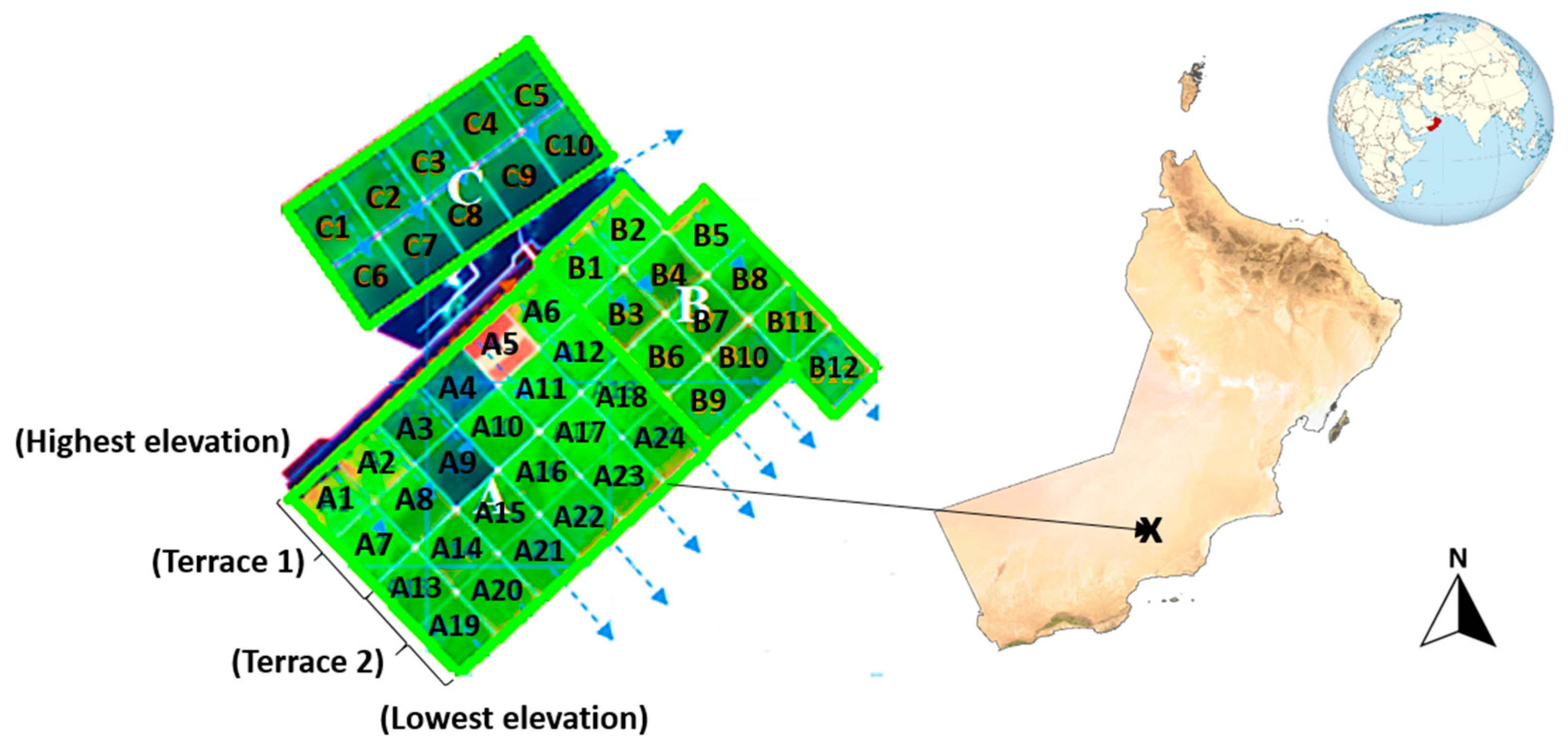
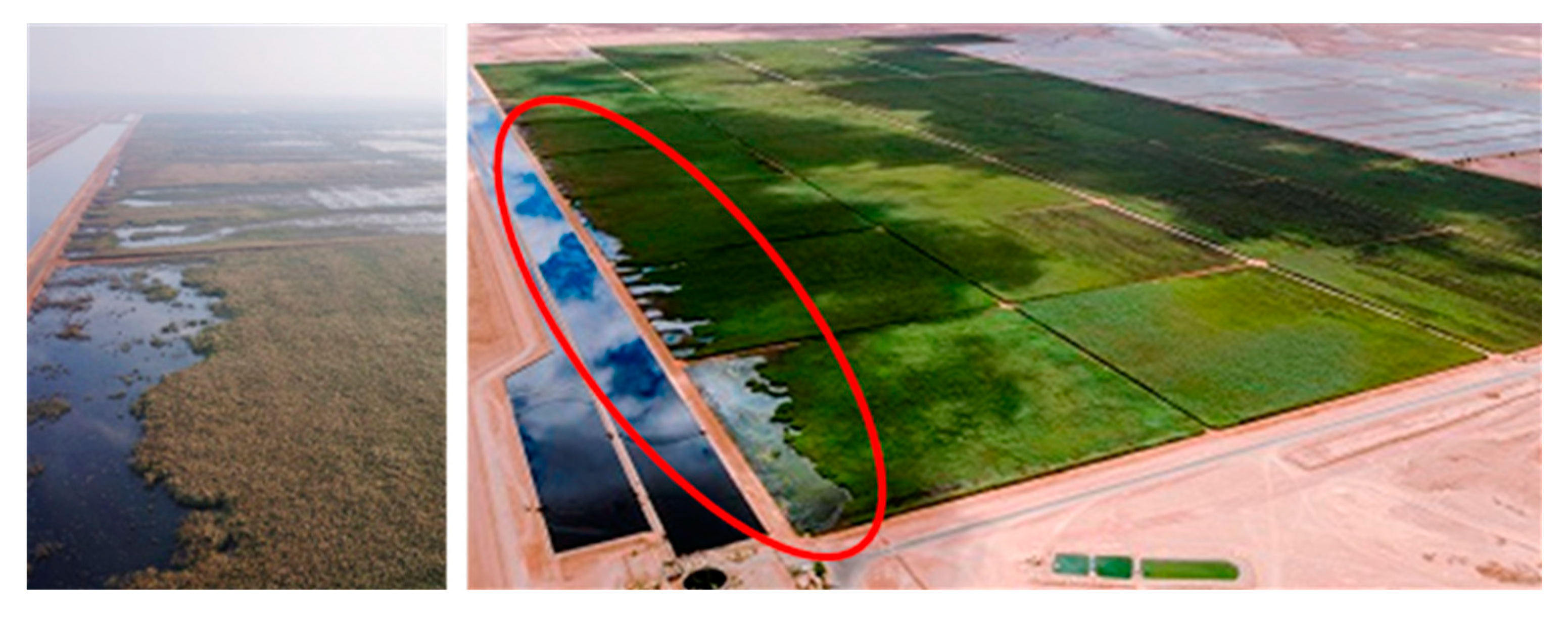
One of the largest CW facilities in the world is in Oman at the Nimr oilfield [
27]. This CW facility receives brackish produced water generated during oil exploration activities in the nearby oilfield. This massive CW in the desert of Oman provides a series of ecosystem services since it represents a green oasis that attracts thousands of migratory birds and improves and regulates the local microclimate [
27]. The CW system has a zero-energy demand for the treatment, since natural treatment processes for the transformation and removal of pollutants occur naturally in this nature-based technology, while gravity flow is applied across the wetland cells. The cells have equal surfaces (approx. 10 hectares each) per the initial design of the facility to distribute the flow equally. The flow enters each cell at the upstream point (from the buffer pond) and flows with gravity along the cell series to the downstream evaporation ponds naturally without the use of an external power; it flows just by using the local topography. To optimize its effectiveness and minimize any negative impact on the environment, a human-made wetland was created based on the natural characteristics of the location. The shape of the wetland was determined by the pre-existing topography, geology, and the amount of available land. The number of cells required for the wetland would depend on factors such as the topography, hydrology, and water quality. In areas with a level surface, cells can be constructed with the use of dikes, while on a sloping terrain, terraced cells can be employed [
28].
The CW is planted with different reed species, making the wetland a polyculture [
16]. Over its 10-year operation, it has been observed that some of the planted reed species had a better tolerance to the water salinity levels and water quality in different seasons than other species that suffered from water salinity stresses at different times of the year and in different locations of the wetland. Furthermore, its indicated that plants thriving in contaminated water are expected to experience greater levels of stress compared to plants growing in unpolluted areas within the same ponds [
29].
The CW facility is located under desert environmental conditions, treating an industrial effluent, while other smaller CWs in the area treat domestic wastewater [
7], highlighting the capacity of this green technology to provide wastewater treatment services under the harshest environments. After more than 10 years of operation and three consecutive expansion phases, today, CW cells cover an area of 490 hectares, followed by 780 hectares of evaporation ponds [
16].
The treatment capacity of the system is 175,000 m³/day, representing about 65% of the total oily produced water generated at that oilfield [
16] or half of the daily water consumption of the Muscat governorate, the capital of Oman [
27,
28]. Various sustainable activities also take place in that facility such as the reuse of the treated effluent for the irrigation of commercial plants, compost production using the reed vegetation, etc.z [
5,
16,
27]. Compared to the previous high-cost and energy-intensive practice of deep well injection for produced water management, the CW system provides not only an excellent treatment (effluent oil-in-water content is below 0.5 mg/L), but also a unique environmental performance, with more than 99% reduced greenhouse gas emissions [
27].
Initially, phragmites australis reeds were planted as the main and only plant species. However, different reed species were later added in the system, such as
Typha domingensis,
Schoenoplectus littoralis,
Juncus rigidus, and
Cyperus spp., to enhance the vegetation production and the resilience and health of the ecosystem. The main biodegradation mechanism is based on cyanobacterial mats trapping oil and degrading hydrocarbons [
30].
The data presented in
Table 1, which was produced by the authors of [
27,
31], demonstrate the effectiveness of the CW system in removing a range of pollutants from the wastewater. The removal of OiW, suspended solids, BOD, and nutrients is attributed to the various physical, chemical, and biological processes that occur within the wetland. The results indicate that CW systems can provide an environmentally sustainable and cost-effective solution for treating wastewater and mitigating water pollution [
27].
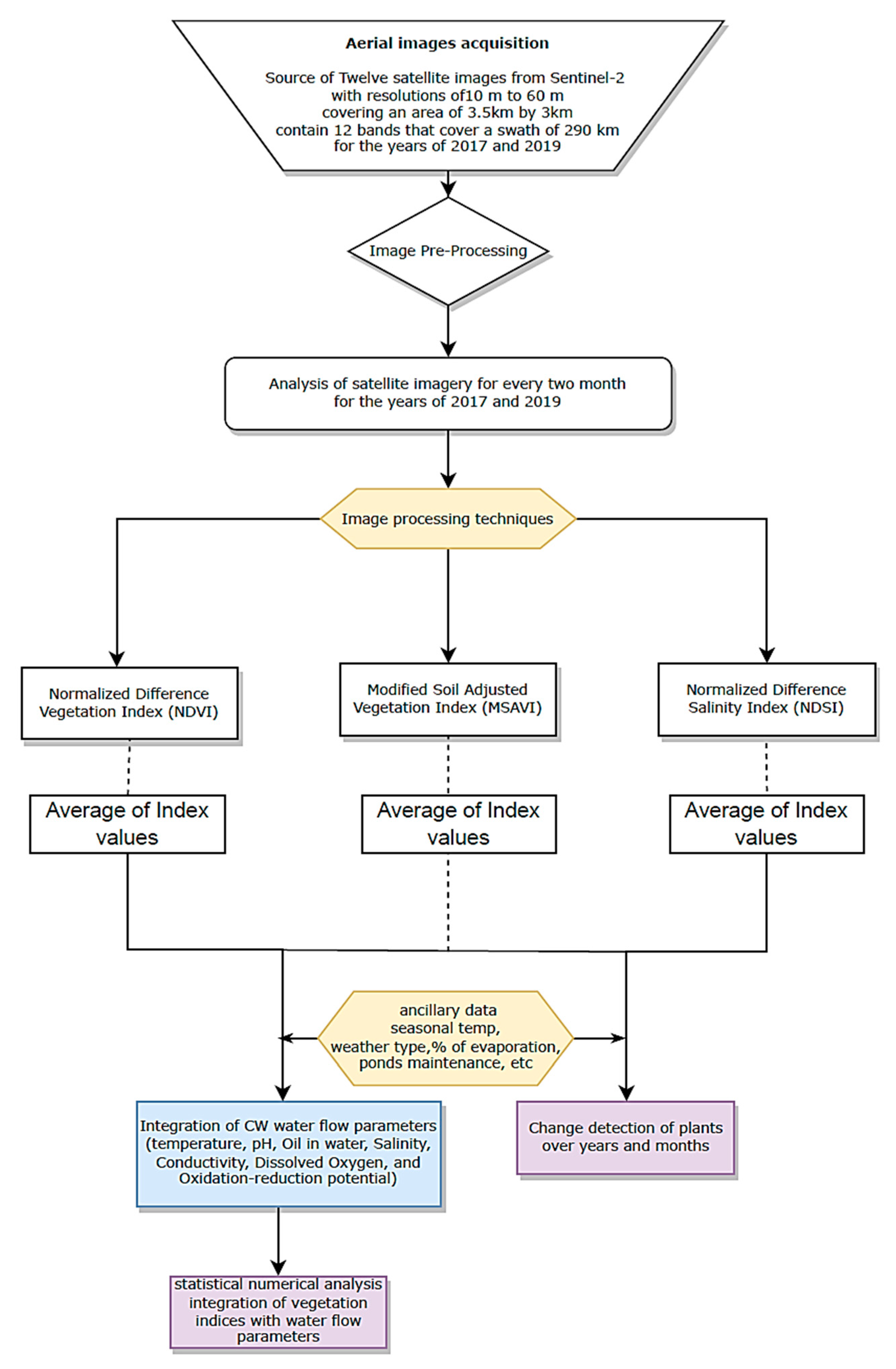
Given the large size of the CW, it is difficult to determine the species that suffered from salinity stress more than others and at what time and place this stress occurred. The use of remote sensing technology can address this difficulty and help in assessing the determination of such reed species temporally and spatially. Moreover, to our knowledge, no remote sensing studies have been conducted on large-scale CW systems or CWs treating oily produced water, especially under a hot and arid climatic region. This study focuses on assessing the health of plants in a massive constructed wetland in Oman. This wetland treats water from oil exploration in a challenging desert environment, exposing the plants to stress from the oil and high salinity. This research examines plant health and changes in the vegetation between 2017 and 2019 using data from Sentinel-2 satellites. Spectral indices including NDVI, MSAVI, and NDSI were used to analyze the plants’ behaviors with these stressors.
Therefore, the objectives of this study were to use remote sensing technology to (1) conduct a change detection analysis for the CW area in Oman, (2) evaluate the performance of the nature-based treatment system in this project, and (3) examine and determine the suffering level of the existing reed species over different seasons of the year.
3. Results and Discussion
3.1. Plant Stress Detection
In this study, an imaging index system was established to appraise plant reactions to stress induced by climatic changes and variations in water parameters across distinct seasons. Employing remote sensing and GIS processing tools along with Microsoft Excel, the imaging data underwent a thorough analysis. This involved the creation of both qualitative false color representations and quantitative graphs, facilitating the discernment of variations in the plant stress levels.
To create a false color image, an initial step involves the generation of a color index file derived from the raw index image. This file preserves the calculated index score for each pixel, denoted as “color index values”. The index scores span from −1.0 to 1.0, with each color index value category corresponding to an incremental range of these index scores. By utilizing this incremental system, an index score of −1.0 denotes an unhealthy status, while a score of 1.0 corresponds to a color index value representing a healthy state. The creation of false color images involves the application of a color lookup table (as illustrated in
Figure 3 and
Figure 4) to the color index file image. These images exhibit artificially generated color schemes that can be customized to highlight pixels with specific color index values in distinct colors, serving the user’s preferences. To produce false color images using the Photo Monitoring plugin, specific settings are applied. These settings involve selecting the option to stretch the near-infrared (NIR) band before generating the index. Additionally, the minimum index value for scaling the color index image is set to −1.00, while the maximum is set to 1.00.
The assessment of plant stress was conducted across various seasons within the specified years, involving a quantitative analysis of the targeted indices juxtaposed with the concurrent calculations of the water flow parameters. This evaluation discerns the impact of high or low scoring index values and their correlations with the water parameters, unveiling the status of healthy or unhealthy plant tissues. Statistical analyses were carried out by employing both Excel’s data analysis tool and the t-test function in R, yielding consistent results. At the conclusion of each year, subsequent to the exposure of targeted ponds, the shift in the peak color index values in the plants exhibited statistically significant differences in comparison to the alterations observed in the peak color index values associated with the water flow parameters.
The dense reed vegetation and the characteristics of the reed clusters make the monitoring and evaluation of each species more challenging with low-resolution mapping images. Therefore, the monitoring and evaluation of the wetland vegetation must be conducted at the scale of the entire reed cluster. In addition, since reed clusters often contain multiple reed species, the differentiation between the different species becomes even more difficult.
Remote sensing methodologies prove to be valuable for detecting alterations in vegetation cover and plant stress, with the spectral indices employed in this investigation (NDVI, MSAVI, and NDSI) demonstrating their effectiveness in capturing information pertaining to salinity, plant stress, and system degradation details induced by produced water. The differences observed between the VSWIR index and other indices indicate the potential of spectral indices to enhance and delineate vegetation stress cover details in an image. The findings of the multivariate analysis conducted on the targeted years indicate moderate saline stress in the wetlands, which is highlighted in the intensity of salinization in different areas depicted in the generated maps. The stressed areas with less vegetation cover can be identified through the remote sensing maps (
Figure 3 and
Figure 4).
The utilization of Sentinel-2 imagery and the spatial resolution of the data, in this study, demonstrated significant effectiveness in accurately delineating the distribution of wetland plant vegetation. To evaluate plant performance in the CW system during the years 2017 and 2019, the similarities and differences between the two years were investigated. The stress on the same cells appeared to be similar in both years, with the plants in the upstream cells close to the produced water inflow exhibiting more stress than those in the downstream cells, as illustrated in
Figure 5 and
Figure 6 for the year 2017.
The cells that showed a weakness in plants growing on their top parts compared to other cells in the CW system were Phase A cells (A1 to A6), Phase B cells (B1, B2, and B5), and Phase C cells (C1 to C5). These cells received inflow with high salinity and hydrocarbon contents, which likely contributed to the observed stress, as indicated by the Vegetation Near-Infrared and Short-Wave Infrared indices.
The research also showed changes in the NDVI and MSAVI indices. The results indicated that the NDVI and MSAVI indices can capture information about plant stress, salinity, and system degradation details. The spectral indices were found to have immense potential in enhancing and delineating vegetation stress cover details in an image. Thus, the Sentinel-2 imagery and the NDVI and MSAVI indices proved to be valuable tools in assessing the response of wetland plant vegetation to changes in the water quality parameters.
3.2. Numerical Analysis
Through the application of laboratory testing on produced water during both the summer and winter seasons, the numerical values of the indices were effectively merged with the corresponding values of the water quality parameters. This integration facilitated a comprehensive understanding of the vegetation conditions prevailing at the CW, thereby providing valuable insights into the complex interactions between the water quality and ecological systems. The outcomes of this approach were instrumental in identifying and assessing the impact of seasonal variations on water quality, as well as enabling the development of informed strategies for sustainable water resource management in the context of the CW ecosystem.
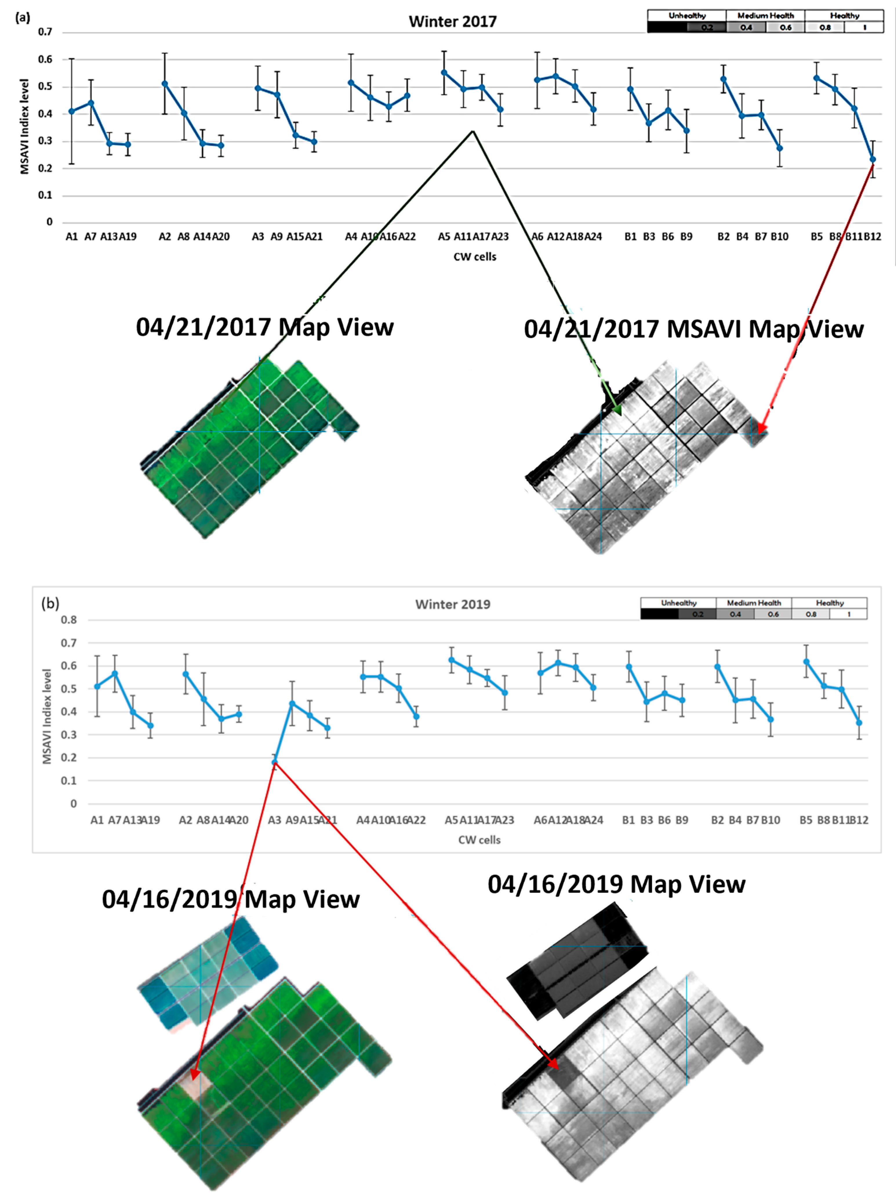
The Modified Soil-Adjusted Vegetation Index (MSAVI) was utilized to rectify the outcomes of the NDVI in the presence of a low vegetative cover and high soil background. By calculating the average maximum MSAVI values of each cell in the CW during both 2017 and 2019, the studied area was classified into three categories based on vegetation health, namely unhealthy for an MSAVI value of <0.3, medium for 0.3 ≤ MSAVI ≤ 0.5, and healthy for an MSAVI value of >0.5. The distribution of the MSAVI served as an example of the classification of plants’ health conditions, as depicted in
Figure 7. Notably, most cells near the outlet exhibited the presence of unhealthy plants under stress due to elevated water salinity levels. Conversely, cells close to the inlet, such as A2, A3, A5, A6, B1, B2, and B5, displayed healthier plants, as inferred from the MSAVI values. This trend was consistent over the two-year period from 2017 to 2019. However, during 2019, some cells malfunctioned, with A3 being out of operation for maintenance reasons, which led to it being dried out. A similar situation was also observed in cells A4 and A9 during the late summer of 2019.
Figure 8,
Figure 9 and
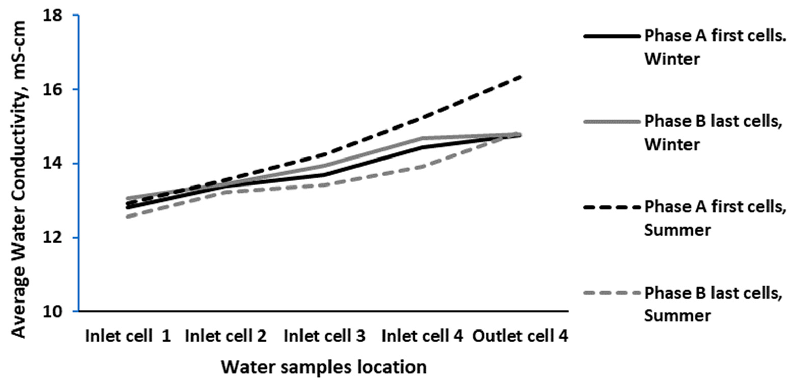
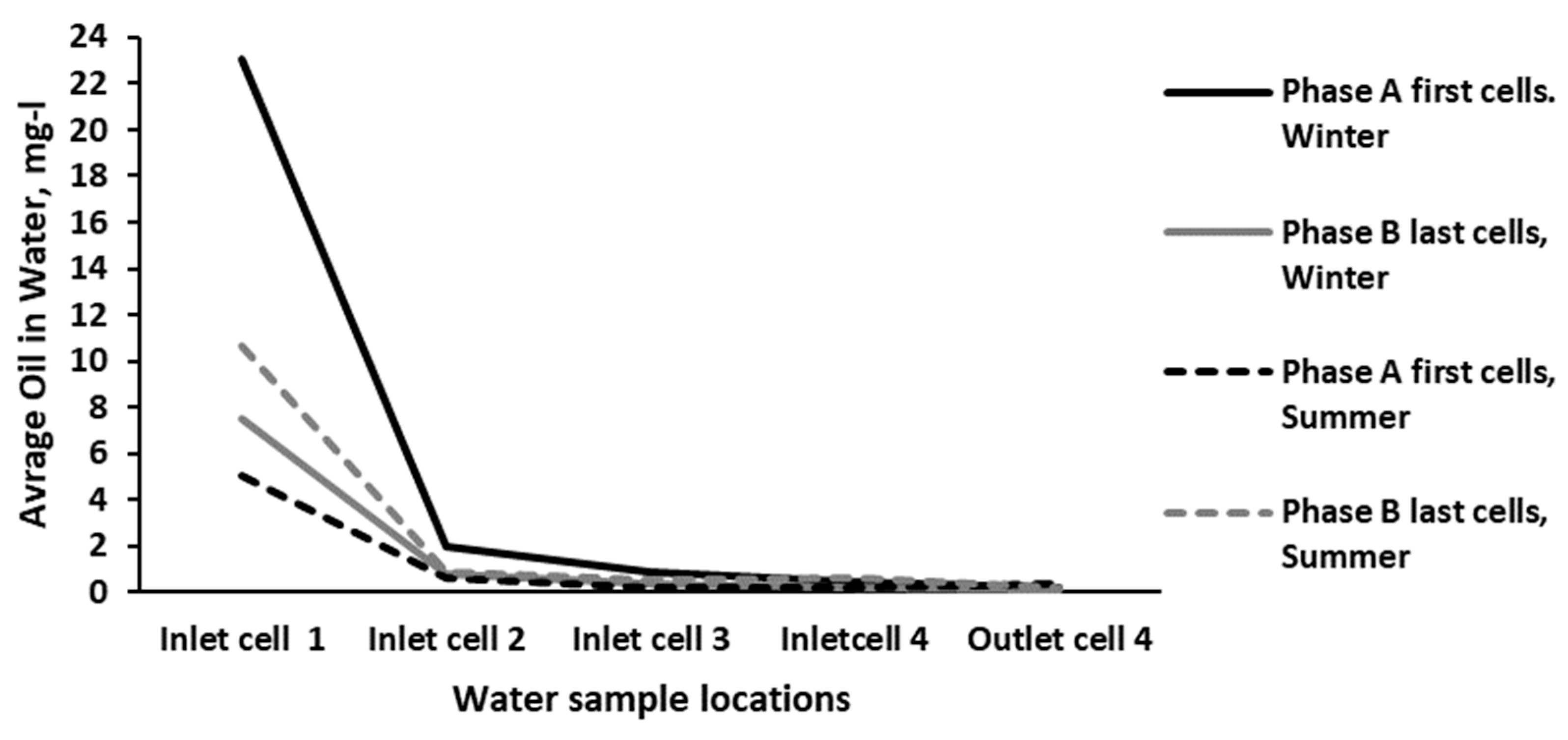
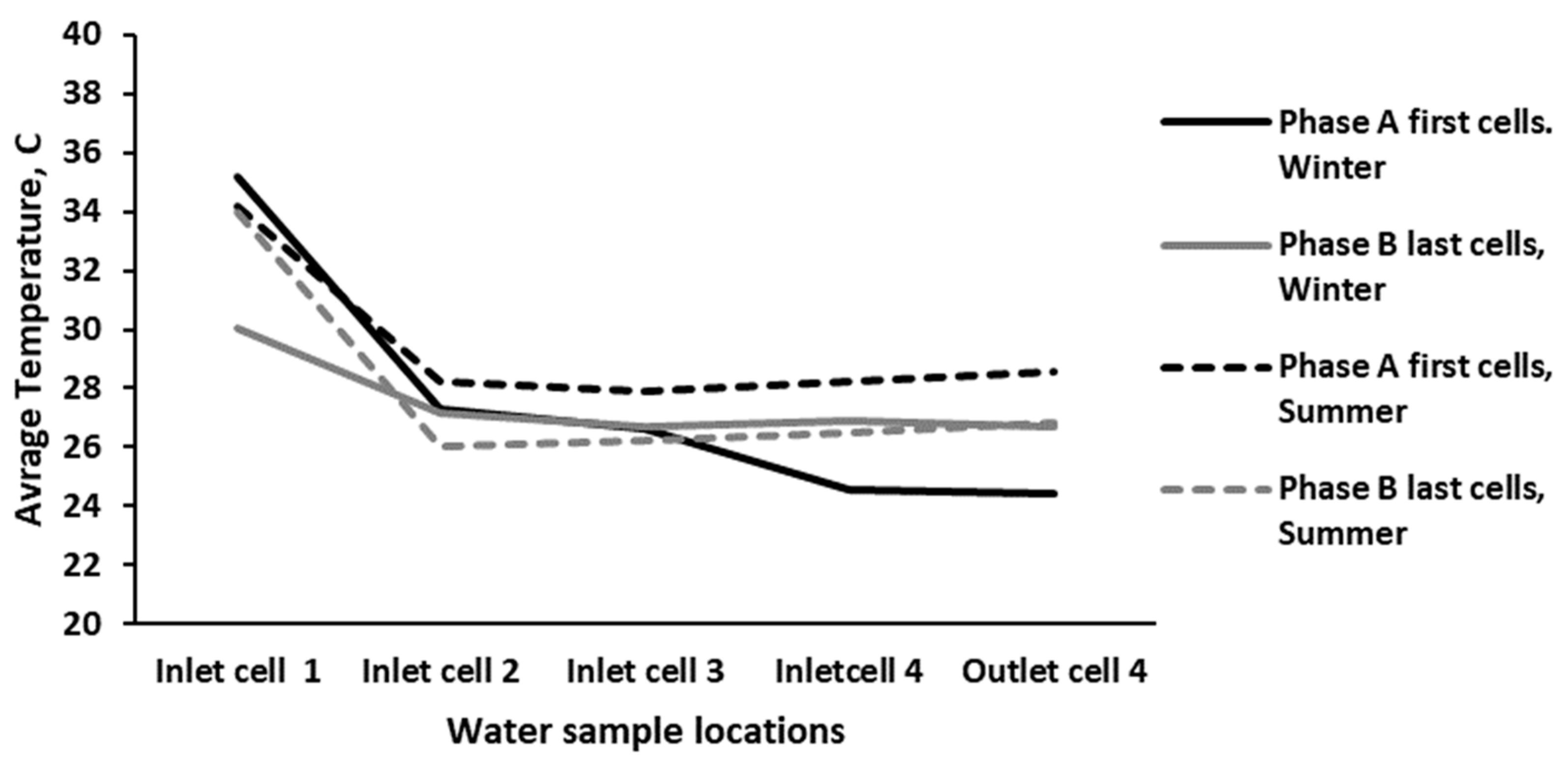
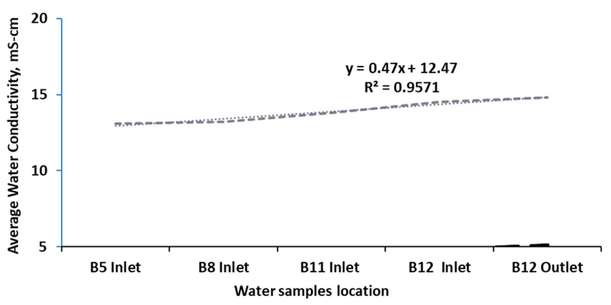
Figure 10 depict the outcomes of the average water flow parameters in the wetland cells of both Phase A and Phase B. The water flow parameters were measured from the first CW cells receiving the produced water inflow to the last cells that discharge water to the evaporation ponds during the winter and summer times of 2017 and 2019. The findings revealed that the water temperature and oil in water (OiW) levels were higher in the inlet CW cells of the first cells, and a subsequent reduction was observed as the produced water flowed towards the last cells in terrace two. Furthermore, the treated produced water showed a further reduction in the temperature and OiW levels upon discharge from the last CW cells to the evaporation ponds. In contrast, the water conductivity levels exhibited an increasing trend as the produced water flowed from the first cells at the first terrace to the last cells at terrace two and subsequently towards the evaporation pond.
The impact of different seasons (winter and summer) on the water flow parameters was assessed for the years 2017 and 2019. The findings revealed that the water temperature levels were higher in the inlet CW cells of the first cells (A1 and B5), whereas a decrease of 3–9 °C was observed as the produced water flowed towards the last cells (A19 and B12) across the reed beds in both evaluated years (
Figure 8). The level of oil contamination in the produced water was similarly reduced by 5–23 mg/L (
Figure 9), and it nearly approached zero as the produced water reached the last cells (A19 and B12), indicating the effectiveness of the CW system. Conversely, the water conductivity levels showed an increase of 2–3 mS/cm as the produced water moved from the inlet at the first cells towards the last cells (
Figure 10).
The data presented in
Figure 11,
Figure 12,
Figure 13,
Figure 14,
Figure 15 and
Figure 16 and in
Table 3 and
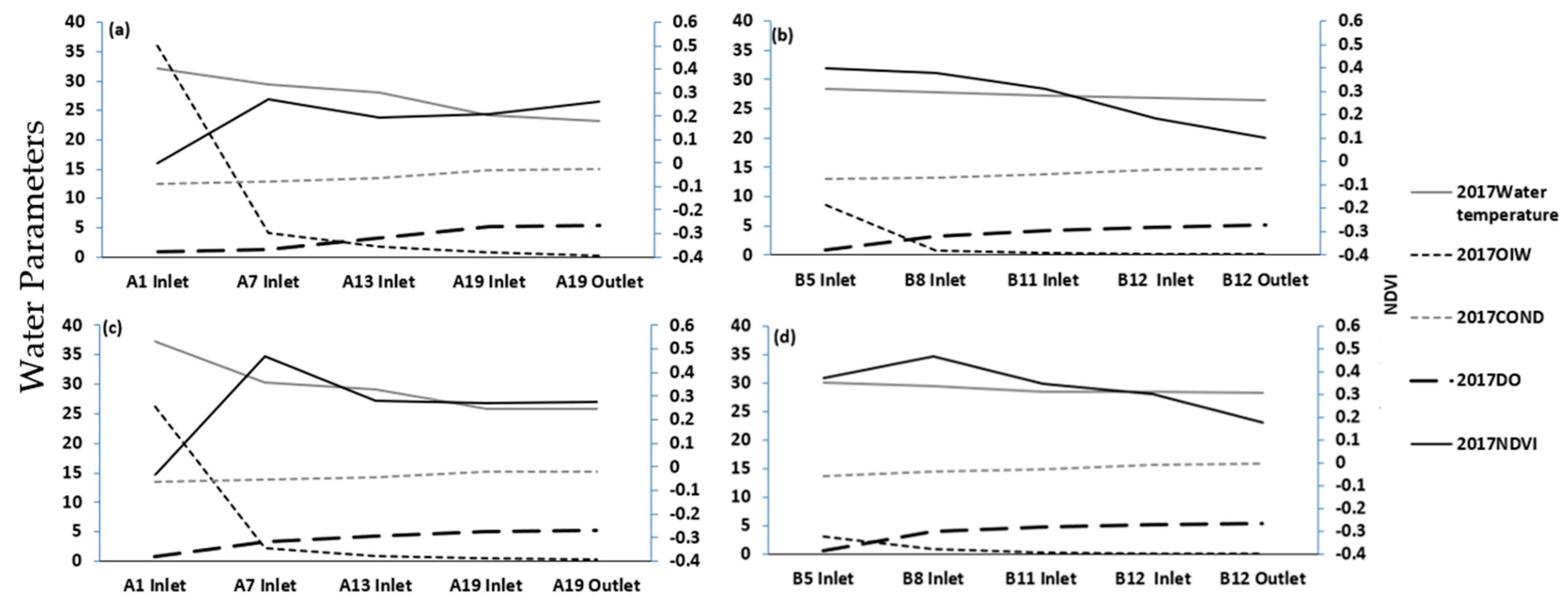
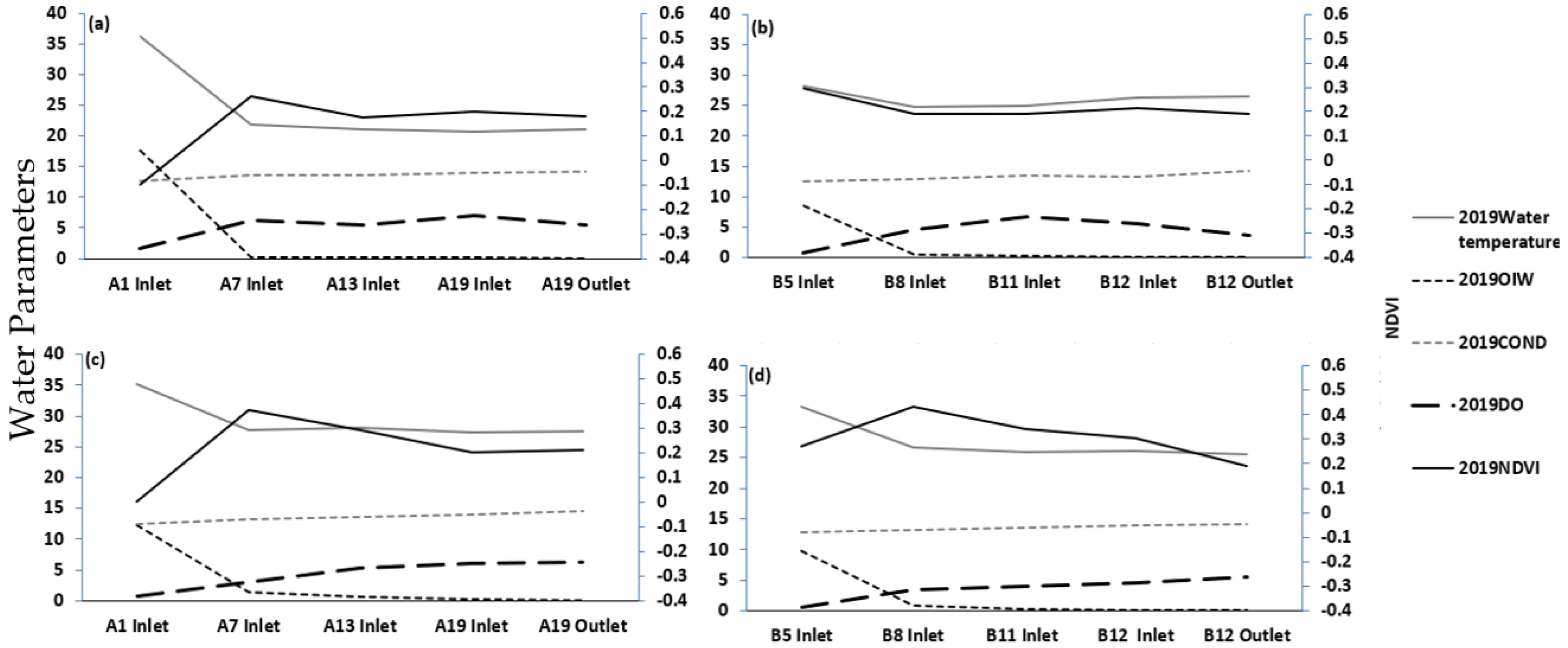
Table 4 demonstrate the influences of various water quality parameters on two seasons in 2017 and 2019, namely the water temperature, oil contamination, water conductivity, dissolved oxygen, and vegetation indices, including the NDVI, NDSI, and MSAVI. The data were collected from the CW tracks of the first cells in Phase A and the last cells in Phase B. The results indicate a positive correlation between the vegetation indices, specifically the NDVI, and water flow parameters. Strong relationships were found between the NDVI and oil contamination in the first cells (A1 to A19) during both seasons of 2017, with an R
2 of 0.87 in the winter and 0.72 in the summer, and 2019, with an R
2 of 0.94 in the winter and 0.66 in the summer. Furthermore, there was a correlation between the NDVI and water temperature in the first cells during the season of 2019, with an R
2 of 0.915 in the winter and 0.704 in the summer (
Figure 12 and
Table 3).
In contrast, the last cells in Phase B (B5 to B12) showed a strong correlation between the NDVI and water conductivity in 2017, with an R
2 of 0.98 in the winter and 0.56 in the summer (
Figure 11 and
Table 4). However, no significant associations were observed in 2019 during any of the seasons for any of the water flow parameters (
Figure 12 and
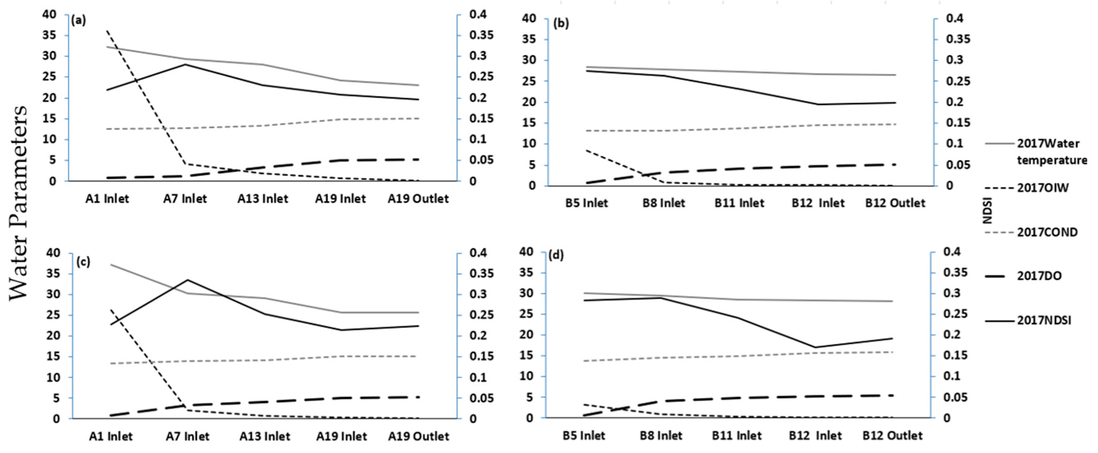
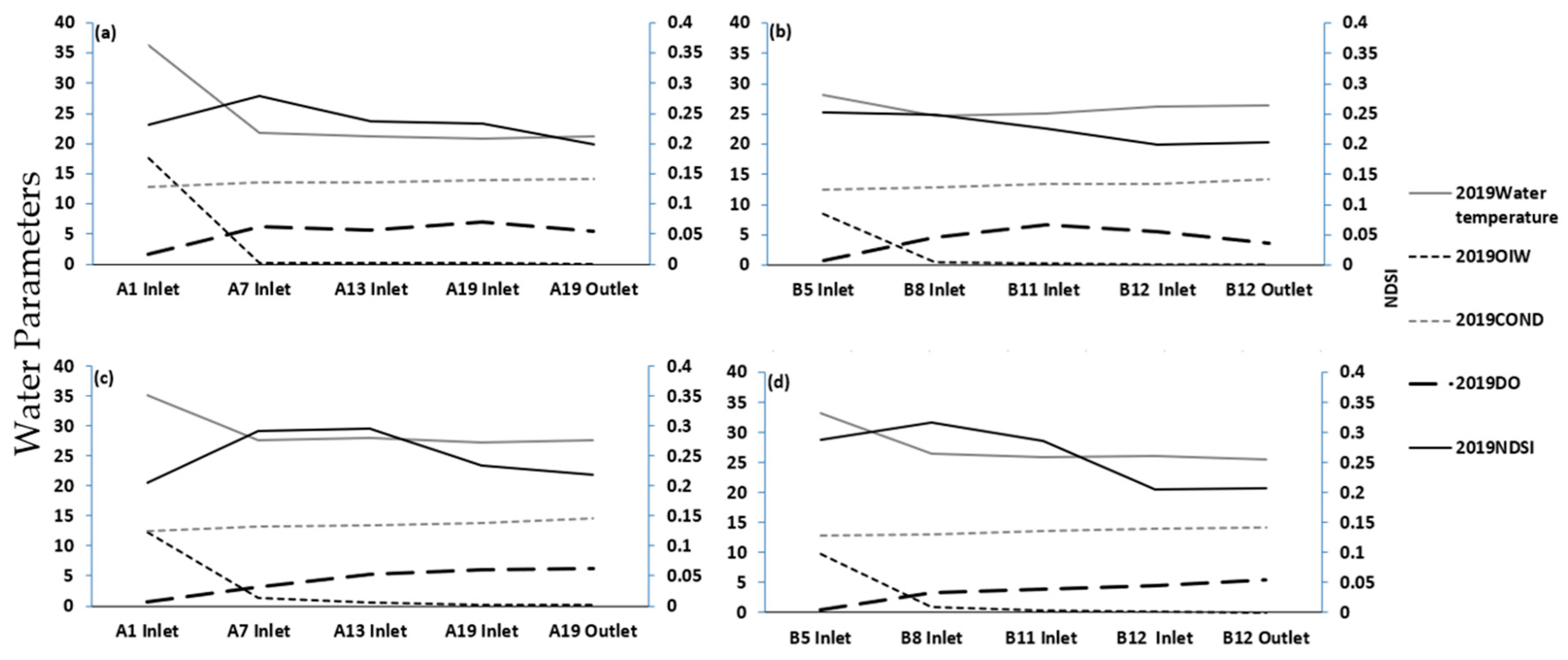
Table 4). Additionally, the NDSI showed a strong correlation with water conductivity in both seasons of both targeted years, 2017 and 2019, with an R
2 of 0.95 in the winter and 0.87 in the summer for 2017 and an R
2 of 0.704 in the winter and 0.766 in the summer for 2019 (
Figure 13 and
Figure 14 and
Table 4).
Overall, these findings suggest that the NDVI and NDSI are useful indicators for water quality assessment and monitoring, particularly in relation to oil contamination and water conductivity, respectively. The results also indicate that the correlation between the vegetation indices and water flow parameters varies depending on the season and location within the CW tracks, emphasizing the importance of considering the temporal and spatial variability when conducting water quality assessments.
The analysis of the vegetation indices (NDSI) in both the winter and summer seasons of the targeted years of 2017 and 2019, along the cells of the CW tracks of the first cells in Phases A did not show significant correlations with the water flow parameters of the first cells (A1 to A19). However, the last cells in Phase B (B5 to B12) exhibited a strong correlation between the vegetation indices (NDVI) and water conductivity in the year of 2017 (R
2:0.95/winter and 0.87/summer) and with the dissolved oxygen in the same year (R
2:0.818/winter and 0.482/summer), as indicated in
Figure 11 and
Table 4. Moreover, the water conductivity demonstrated a correlation between the last cells in Phase B (B5 to B12) and the NDSI indices in the year of 2019 (R
2:0.70/winter and 0.766/summer), as presented in
Figure 14 and
Table 4. These findings suggest that the NDVI and water conductivity are useful indicators for water quality assessment and monitoring in the last cells of Phase B. However, the NDSI did not show any significant correlations with the water flow parameters in the first cells of Phase A.
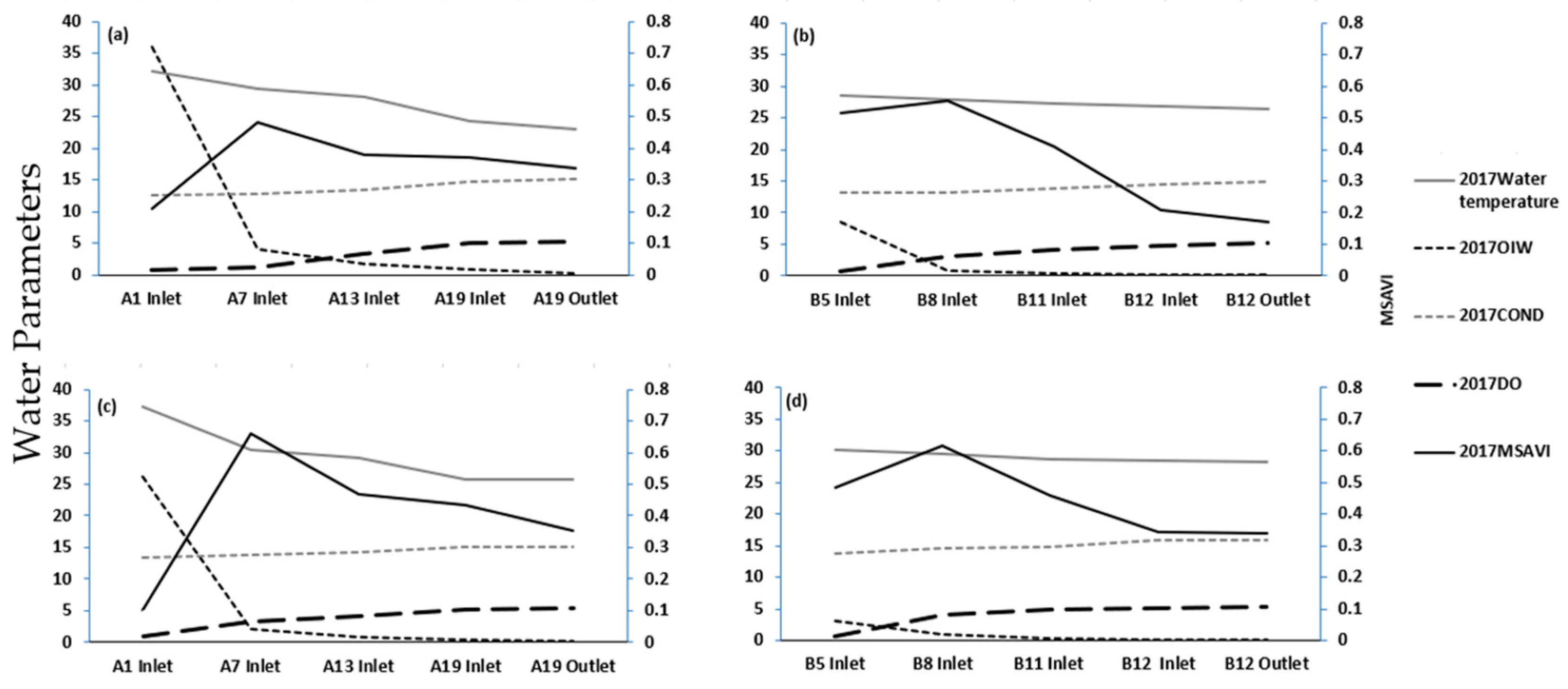
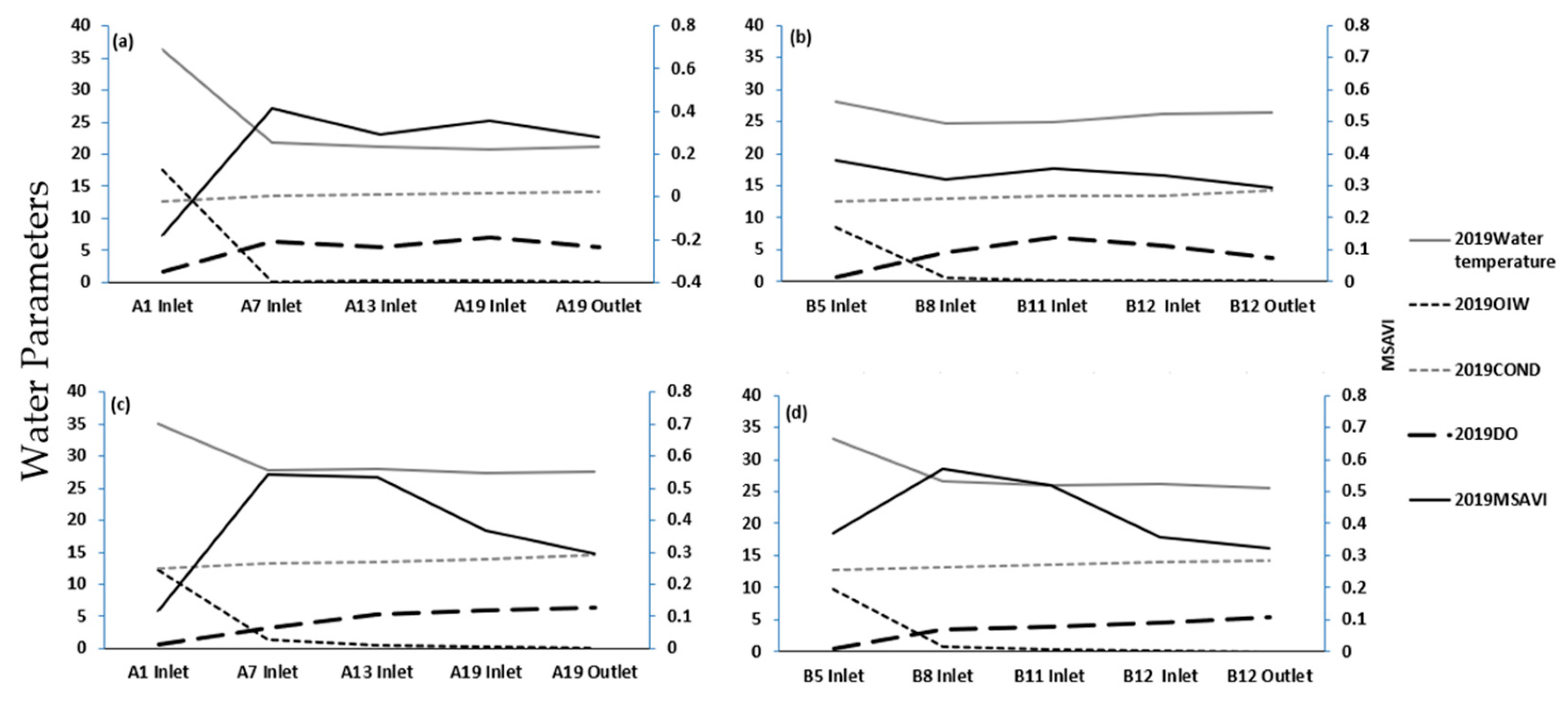
The Modified Soil-Adjusted Vegetation Index (MSAVI) was evaluated for both seasons (winter and summer) of the years 2017 and 2019 along the cells of the CW in Phase A and the last cells in Phase B. The results showed that the MSAVI is correlated with the OIW flow parameters of the first cells (A1 to A19) in both years in Phase A with the R
2 values of 0.608 (winter) and 0.626 (summer) in the year of 2017, and R
2 values of 0.947 (winter) and 0.567 (summer) in the year of 2019, as shown in
Figure 15 and
Figure 16 and
Table 3 and
Table 4.
Moreover, the last cells in Phase B (B5 to B12) showed a good correlation between the MSAVI and water conductivity in the year of 2017 with R
2 values of 0.977 (winter) and 0.5866 (summer), and in the year of 2019 with R
2 values of 0.568 (winter) and 0.218 (summer), as shown in
Figure 15 and
Figure 16 and in
Table 3 and
Table 4.
The findings of the study suggest that both the MSAVI and NDSI exhibited similar reflectance correlations with the water flow parameters. The MSAVI was found to be useful in correcting the outcomes of the NDVI by accounting for the influence of the soil background, especially in areas with a low vegetation cover. Additionally, the NDSI was effective in identifying the salinity stress on reed plants and was able to capture this stress through the correlation between the NDSI and water conductivity in the last cells of Phase B (B5 to B12). These results are presented in
Figure 13 and
Figure 14 as well as in
Table 3 and
Table 4.
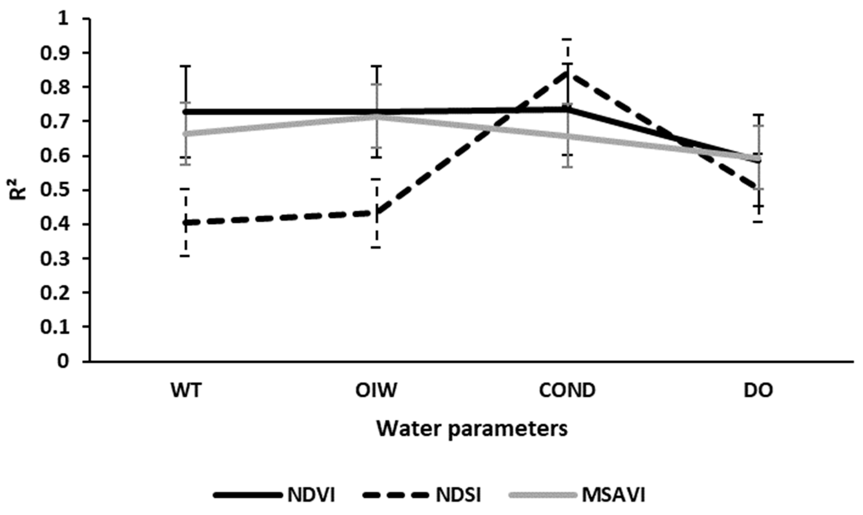
Figure 17 and
Figure 18 and
Table 3 and
Table 4 provide an overview of the R
2 values obtained for the water collection parameters in both 2017 and 2019 for the winter and summer seasons. The results highlight the usefulness of the correlation indicators in water quality assessment and monitoring. The figure indicates that the vegetation index NDVI showed higher average R
2 values compared to the other parameters (
Figure 18).
3.3. Discussion
The CW system is responsible for a significant increase in the total dissolved solids (TDS) concentration in the effluent. The high TDS concentration is attributed to the large surface area of the CW and the dense reed vegetations that result in high water losses through evapotranspiration [
27]. The inflow TDS concentration is around 7–8000 mg/L, while the effluent TDS concentration exceeds 12,000 mg/L [
28]. As the water flows with gravity from the upstream to the downstream wetland cells, a gradual increase in salinity is detected. Boron, which is relatively high in concentration in the inflow (
Table 1), might also have an impact on plant growth, along with salinity. However, the boron levels generally remain lower than the reported level, which might induce phytotoxicity (i.e., 7 mg/L) [
27]. Despite these conditions, the reed plants manage to survive and grow well, establishing, in time, a rich vegetation with a high density.
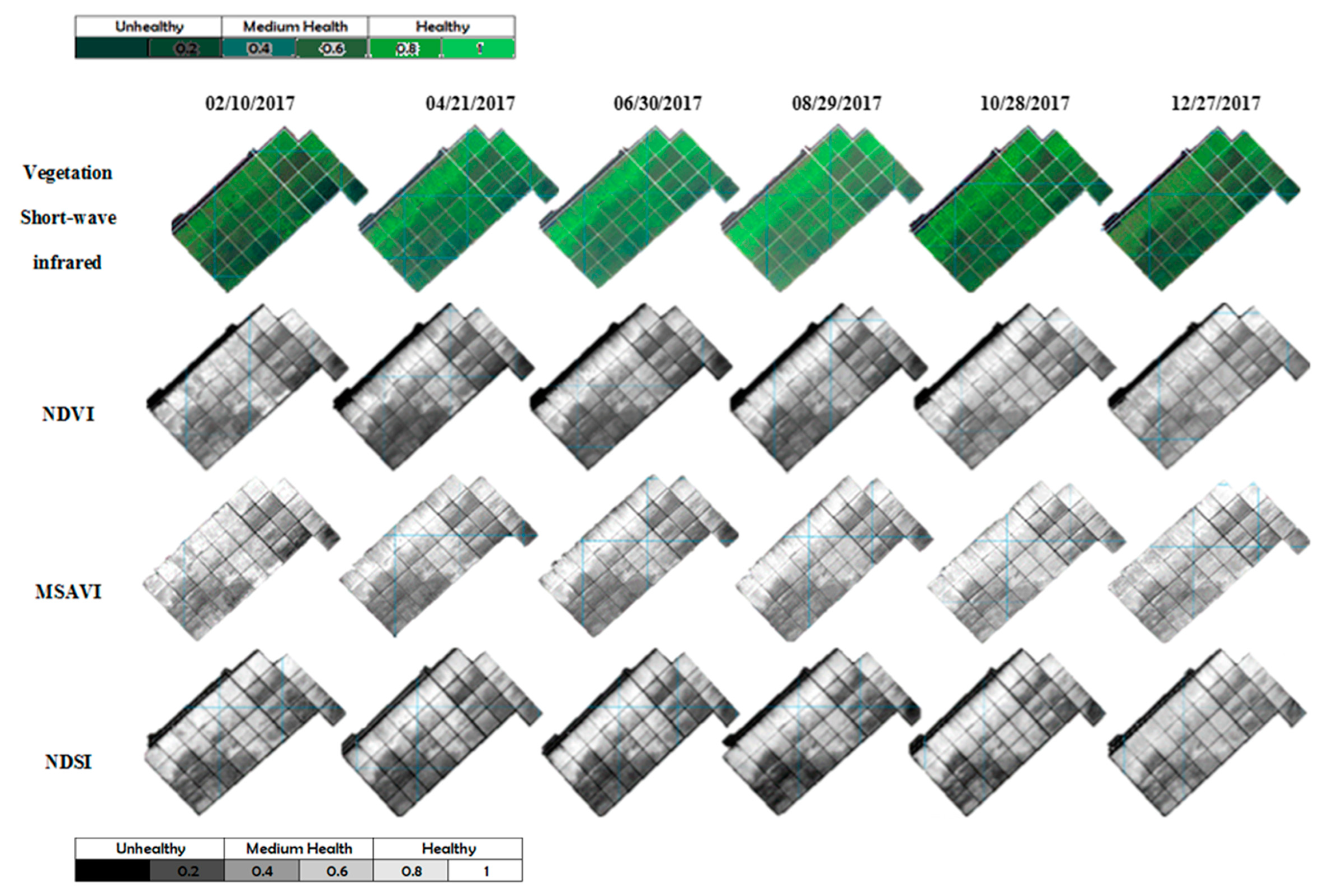
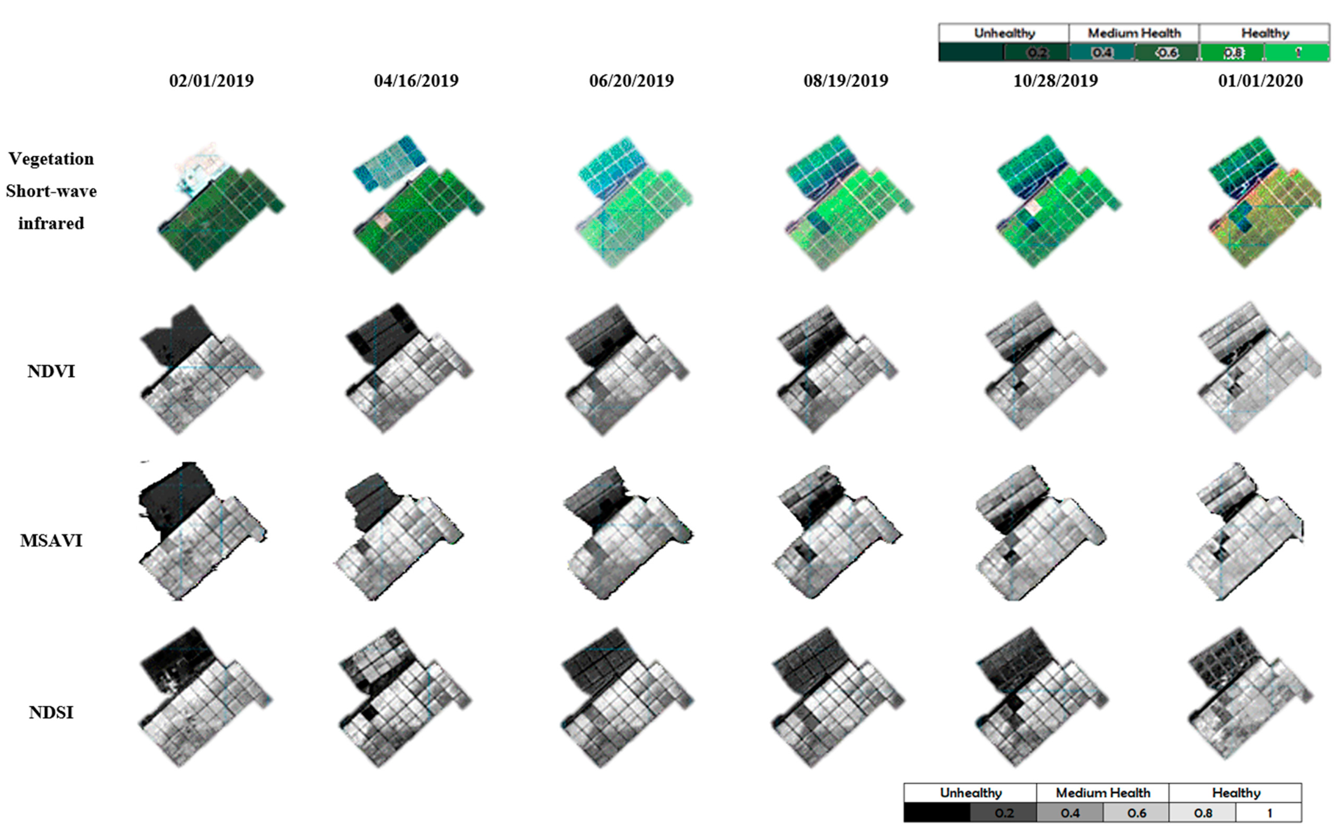
Figure 3 and
Figure 4 present a bi-monthly estimation of plant stress change detection in the CW for the years 2017 and 2019. The analysis was conducted using the Vegetation Short-Wave Infrared (VSWIR) index and spectral indices (NDVI, MSAVI, and NDSI) obtained from Sentinel resolution imaging. The outcomes of the change detection analysis revealed noteworthy alterations in the vegetation cover within specific cells and more subtle variations in the others, alongside changes in the land cover during the two designated years. Concretely, cells A3, A4, A9, A10, A13, A15, A16, A19, A21, and A22 in Phase A demonstrated disparities between the two years, while the downstream cells of Phase B, specifically cells B8, B10, B11, and B12, displayed detectable changes.
The produced water samples were taken at the inlet of the cells and at the outlet of the last cells, with the first cells starting from A1, A7, A13, and A19 and leaving to the evaporation ponds, while the inlet of the last cells of phase B starts at B5, B8, B11, and B12 and leaves to the evaporation ponds.
The average content of oil in water (OiW) in the inflow was found to be approximately 280 mg/L, with occasional spikes that exceeded 500 mg/L, as reported in earlier studies [
27,
28]. However, the treatment process in the CW system resulted in a significant reduction in the OiW, with levels dropping to below 0.5 mg/L in the treated effluent. The average concentration of suspended solids was reduced from 28 mg/L in the inflow to 10 mg/L in the treated effluent, while the average BOD concentration dropped from 16 mg/L to less than 1 mg/L. This reduction in the BOD is particularly noteworthy, as it indicates the removal of biodegradable organic matter from the wastewater.
The CW system also showed an efficient removal of nutrients, such as nitrogen and phosphorus, which are typically found in wastewater. However, the concentration of these nutrients in the inflow was already low, with the levels not exceeding 2–3 mg/L. Consequently, the treated effluent did not have measurable concentrations of nitrogen and phosphorus.
During the operational lifespan of the wetlands, a discernible observation emerged, indicating that certain reed species, when compared to others, exhibited heightened resilience to varying water salinity levels and fluctuations in water quality across different seasons and diverse locations within the wetland. Conversely, several other species encountered challenges due to water salinity stresses, displaying susceptibility at different periods throughout the year and at various sections within the wetland [
16]. The analysis of change detection in the constructed wetland (CW) in Oman provided valuable insights into the variations in wetland stress across the specific seasons and years under examination. The wetland showed that plants could be grown economically with irrigation-treated water of up to EC 16 mS cm (
Figure 8). The greater application of produced water positively affected plant growth by accumulating a toxic level of salts in the lower soil horizons. The use of diluted seawater for barley irrigation is only possible if the leaching of excess salt from the root zone is implemented. However, the soil and plant data found in this study were in the same line of many published data, where the plants underwent stress as the salinity, temperature, and oil in water increased [
15].
In addition to employing indices pertaining to the chlorophyll content, the integration of water flow parameters played a pivotal role in the estimation of various botanical attributes, encompassing photosynthetic pigments, water, nitrogen, and leaf mass per area (e.g., NDSI) [
34]. Consequently, the inclusion of vegetation indices exerted a more pronounced impact on the classification results compared to the original short-wave infrared reflectance. Nevertheless, discernible distinctions in relative importance emerged among the three tested indices (NDVI, NDSI, and MSAVI). The computed importance values, denoted by R
2, served as valuable indicators when correlating the indices with water flow, leading to a substantial enhancement in the accuracy of identifying stressed croplands. The research utilized cost-free satellite images to evaluate stress in reed grass plants induced by hydrocarbon water flow contamination within the wetland. Moreover, the study area experiences an extremely harsh climate, making it uncommon to find comparable research references for the assessment of spectral indices. A higher spectral resolution sensor image could potentially provide a more accurate estimation of the stress content in the plants [
29].
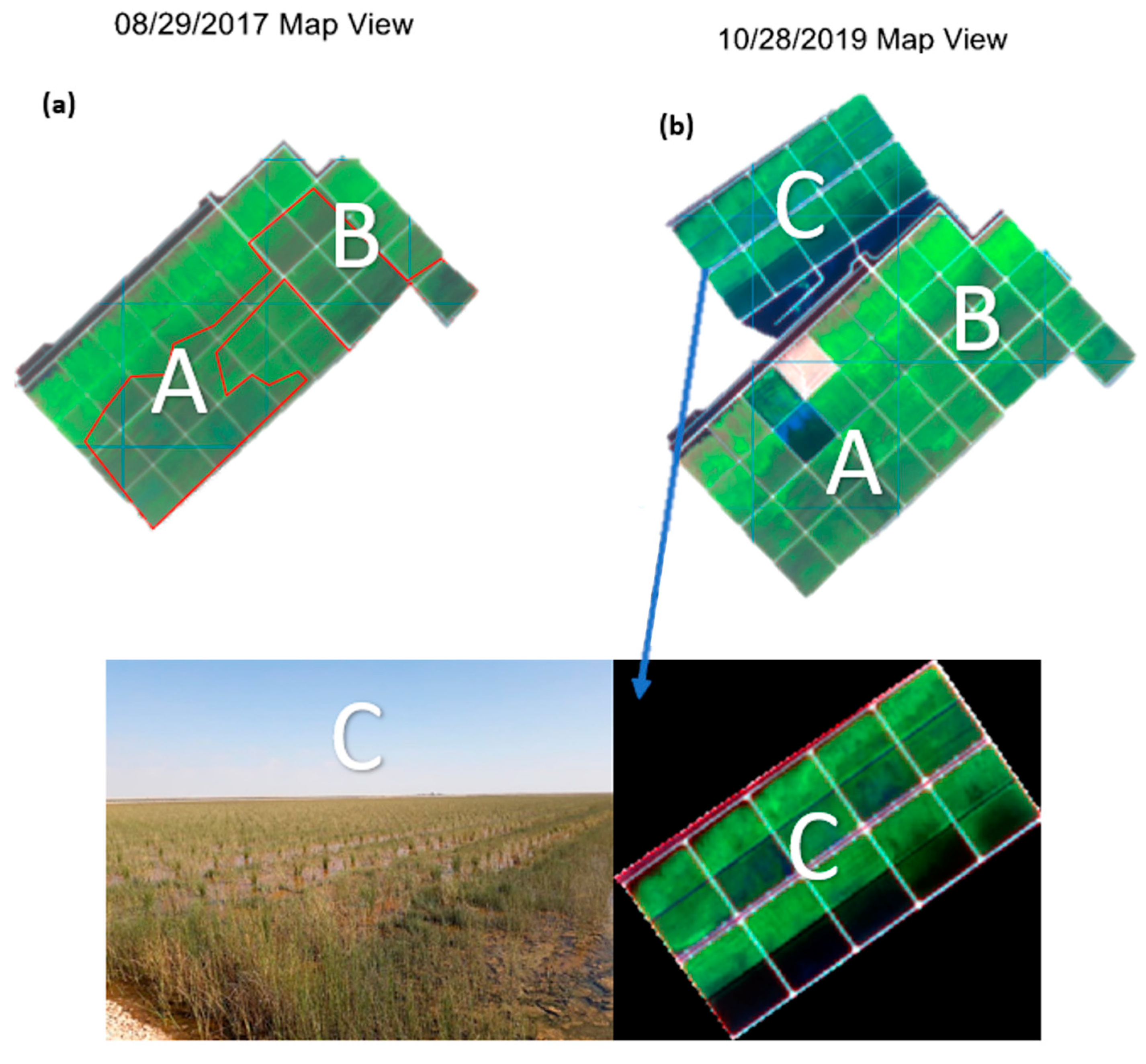
In the third phase (C) of the study, which involved the cultivation of new plants, it was observed that the same stress challenges associated with inflowing water were present. This was evidenced by the appearance of stress on the new CW cells of Phase C within four months of planting, as was also observed in Phases A and B, regardless of the plant species. These findings highlight the presence of high levels of salinity and hydrocarbon stress during the first stage of produced water inflow. In addition, the NDVI and MSAVI revealed variations in plant health across Phase A and Phase B cells, with some cells exhibiting higher levels of vegetation stress than others, as illustrated in
Figure 5 and
Figure 6 for the year 2017. However, when new reed species were planted in Phase C, it was difficult to determine definitively whether the impact of produced water inflow stress on the plants was high or low within a year’s time. As such, further investigation is necessary in Phase C to detect stress more comprehensively on the plants.
This study represents a measure towards the potential of remote sensing in the treatment of hydrocarbon-contaminated water in wetlands via using correlation indicators in water quality assessment and monitoring. The vegetation indices showed their usefulness as tools for assessing water quality and monitoring the impact of various water quality parameters on the environment. By analyzing the R2 values, it is possible to determine the extent to which changes in the water quality parameters affect the vegetation index, which can help identify areas that require further investigation and remediation efforts. These findings have significant implications for environmental monitoring and management, as they provide a valuable means of assessing the impact of water quality on the environment and identifying areas that require targeted interventions to improve the water quality.
In addition, the use of correlation indicators such as the NDVI can help identify the specific water quality parameters that are affecting vegetation growth and health. This information can be used to inform targeted interventions that address the specific water quality issues in each area. Furthermore, the use of correlation indicators can help prioritize areas for further investigation and remediation efforts, which can be particularly useful in resource-limited settings.
The findings of this study suggest that correlation indicators such as the NDVI can be a valuable tool in water quality assessment and monitoring. By identifying areas that require targeted interventions, these indicators can help improve environmental management and protect ecosystems from the negative impacts of poor water quality.


