Spatio-Temporal Dynamics of Total Suspended Sediments in the Belize Coastal Lagoon

Abstract

Increased tourism in Belize over the last decade and the growth of the local population have led to coastal development and infrastructure expansion. Land use alteration and anthropogenic activity may change the sediment and nutrient loads in coastal systems, which can negatively affect ecosystems via mechanisms such as reducing photosynthetically active radiation fields, smothering sessile habitats, and stimulating eutrophication events. Accurate monitoring and prediction of water quality parameters such as Total Suspended Sediments (TSS), are essential in order to understand the influence of land-based changes, climate, and human activities on the coastal systems and devise strategies to mitigate negative impacts. This study implements machine learning algorithms such as Random Forests (RF), Extreme Gradient Boosting (XGB), and Deep Neural Networks (DNN) to estimate TSS using Sentinel-2 reflectance data in the Belize Coastal Lagoon (BCL) and validates the results using TSS data collected in situ. DNN performed the best and estimated TSS with a testing R² of 0.89. Time-series analysis was also performed on the BCL’s TSS trends using Bayesian Changepoint Detection (BCD) methods to flag anomalously high TSS spatio-temporally, which may be caused by dredging events. Having such a framework can ease the near-real-time monitoring of water quality in Belize, help track the TSS dynamics for anomalies, and aid in meeting and maintaining the sustainable goals for Belize.

1. Introduction

1.1. Ecological Significance of the Belize Coastal Lagoon

The Mesoamerican Caribbean Region is home to the second-longest barrier reef in the world, with approximately 30% of this reef structure running the length of the coastline of Belize. The Belize Barrier Reef System (BBRS) comprises the Belize Coastal Lagoon (BCL), three atolls: Turneffe Atoll, Lighthouse Reef Atoll, and Glover’s Atoll, and a complex of Marine Protected Areas (MPAs) that span these reef areas. Nested within this expansive complex of reefs is a UNESCO World Heritage site known as the Belize Barrier Reef Reserve System (BBRRS), featuring a selection of seven MPAs with a diverse collection of flora and fauna.

1.2. Economic Importance of the Belize Coastal Lagoon

A significant portion of the population of Belize depends on the agriculture, fishing, and eco-tourism industries for employment opportunities [1]. A 2009 study conducted by the World Resource Institute (WRI) estimated that the total annual values of the coral reef and mangroves in the BBRRS were between USD 396 and USD 559 million per year, and the Belize coastal lagoon accounted for 12–15% of Belize’s gross domestic product (GDP) [2]. The 16 significant watersheds in Belize directly impact the coral reef health and biodiversity in the BCL by dispersing eroded sediments and nutrients [3,4]. Coral reef ecosystems attract a thriving collection of aquatic biodiversity and provide habitat to support approximately 550,000 to 1,330,000 species [5,6]. Essential for the communities living around them, coral reefs provide protection from coastal erosion and hurricanes and opportunities for commercial fishing, recreation, and eco-tourism [4].

1.3. Sedimentation Issues and the BCL’s Water Quality

Total suspended sediments (TSS) are composed of organic and inorganic materials [7,8] and are introduced to water bodies through runoff, dredging activities in coastal waters, and resuspension events [7]. The introduction of large amounts of sediments to marine environments can negatively impact ecosystems as they may contain harmful materials such as heavy metals, pollutants, or high nutrient loads [9]. Since suspended sediments are optically active constituents, they may decrease the penetration of light through the water column [7,9,10]. This, in turn, can impact primary production levels and, therefore, alter the ecosystem in that area [7].

Suspended sediment settling on coral reef ecosystems can hinder biological processes [11,12,13,14,15,16]. Large sediment loads impede reef development because coral cannot recruit onto silt, mud, or sand, given that they require hard substrates to attach to. When sediments settle on established coral colonies, coral polyps must self-clean their surface via ciliary action, mucus production, or hydrostatic polyp inflation methods. These mechanisms are metabolically expensive for the corals and negatively affect their health [12,17,18,19,20]. Sediment plumes also increase turbidity and result in lower light levels. The combination of the high energetic requirement for self-cleaning, the corals’ inability to open their polyps, and the photosynthetic nature of their symbiotic zooxanthellae lead to a reduction in the corals’ ability to feed [13,19], potentially causing coral starvation and reduced calcification [18,21,22,23,24,25,26].

1.4. Remote Sensing of TSS

TSS concentration in seawater has traditionally been quantified by laboratory analysis of samples collected from the field. However, point-based field sampling alone is an impractical method for quantifying the long-term spatial dynamics of TSS, given that it is expensive, time-consuming, and dependent on access to the field site. As an Optically Active Component (OAC), TSS alters the spectral characteristics of water, making remote sensing a viable alternative to monitor it [10]. Remote sensing applications circumvent the barriers of traditional sampling, such as human efforts and field and equipment costs for continuous monitoring, and provides the ability to monitor water bodies over significantly expanded spatial and temporal scales [10].

Traditional empirical models for TSS estimation use remote sensing reflectance (Rrs) of single bands or a combination of bands and are highly suitable for a limited range of TSS concentration [7]. For instance, Ouillon et al. (2004) in New Caledonia [27], Miller and McKee (2004) in the Mississippi River Delta [8], Kumar et al. (2016) in Chilika Lake, India [28] and in the Chesapeake Bay [29], used methods including linear regression and high order polynomials of single band models to estimate TSS concentrations. However, these models perform poorly in areas with highly variable TSS concentration ranges or low TSS concentrations [30,31,32,33].

1.5. Summary and Objectives

Considering the landscape and geographic location and the total precipitation and runoff output of the BCL, it can be theorized that land-based parameters contribute to changes in TSS levels in the BCL. The BCL is home to mangroves, seagrass, and coral reef habitats. These features show up in satellite images as areas that are darker than the surrounding water, and such benthic habitats can confuse traditional empirical models and lead to the overestimation of TSS levels. Radiometric sensitivity is crucial for clear water conditions, such as in the BCL, where benthic reflectance poses a challenge for accurate water quality modeling. Therefore, it is important to create a model that will be able to account for these habitats and avoid overestimation of TSS levels due to interference from benthic habitats. With that, this study puts forth the following specific objectives: (i) A comparative study of Machine Learning (ML) algorithms to model the TSS concentration in the optically complex BCL using satellite-based surface reflectance, and (ii) A comprehensive time-series trend analysis using Bayesian and statistical methods of changepoint detection, to develop the relationship between TSS concentration trends and parameters such as precipitation and runoff. This can help understand spatio-temporal patterns of TSS in the BCL and its potential drivers that may be causing anomalous TSS concentrations. Additionally, having a TSS estimation model that is able to predict a highly variable range of TSS concentrations may be used in different study areas without being bound by the limitations of site-specificity.

2. Materials and Methods

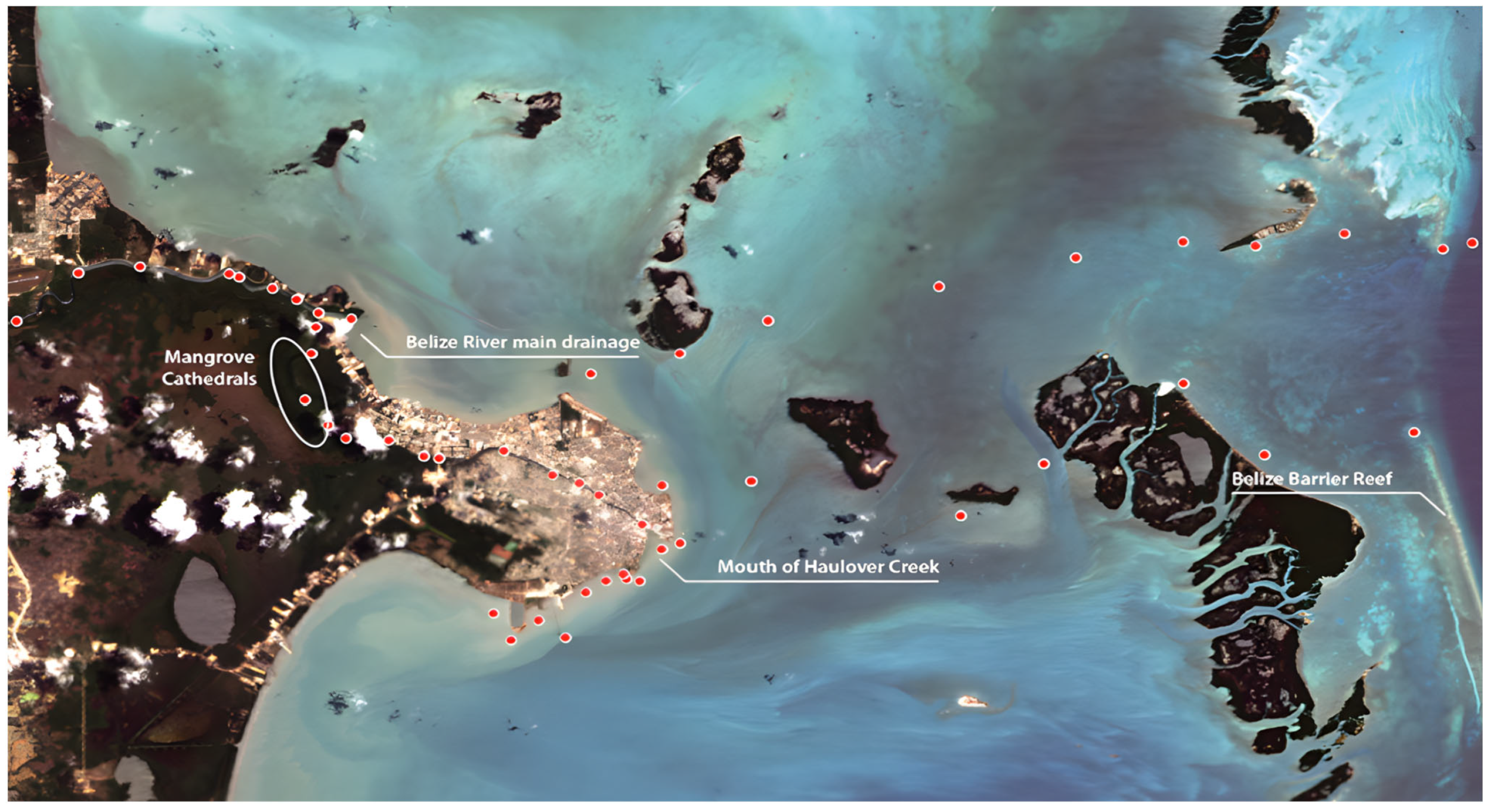
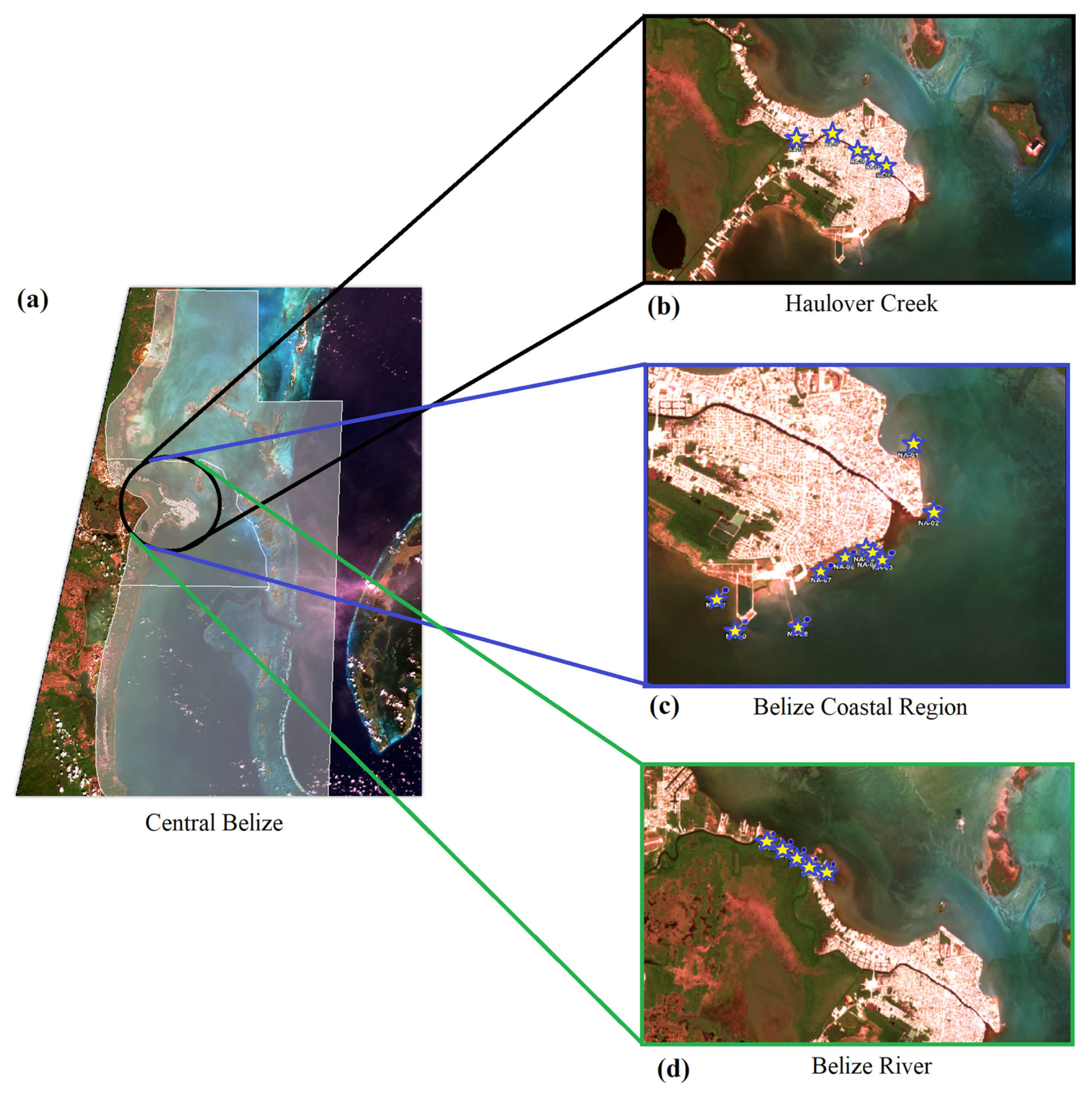
2.1. Study Site

The study area in the BCL contains a total of 50 sampling sites that are located in the central portion of the Belize Barrier Reef Lagoon (BBRL), proximal to Belize City (Figure 1). Belize City is located south of the mouth of the Belize River on a delta that is surrounded by mangroves and the Caribbean Sea. Haulover Creek, known as the inlet of the Belize River, runs through the center of Belize City and opens up to the BBRL. This area is surrounded by factories and communities and is in close proximity to the cruise tourism village in Belize City. This region experiences high marine traffic and is the site for the disposal of waste and treated and untreated sewage directly from the Belize City watershed. The area where the Haulover Creek opens out to the BBRL is also a port for coastal ferries and small fishing vessels. A region of Haulover Creek also passes through the middle of Belize City and experiences high boat traffic and sewage disposal from nearby communities. The existence of the port makes the region susceptible to high suspended sediment concentrations due to resuspension events caused by the boat movements and their motors, as well as regular dredging activity [34,35]. Field sampling was conducted in several locations along Haulover Creek, going out to the BBRL and out to the Barrier Reef.

2.2. Data

2.2.1. Field Data

Field sampling took place in the BBRS during the dry season months from 2019 to 2021. The field data for TSS modeling consisted of water samples to estimate TSS concentrations, depth readings, and YSI measurements that consisted of conductivity, pH, temperature, salinity, and dissolved (DO) readings. Additionally, a separate field campaign was conducted in November 2018 by the National Oceanography Center in the UK in collaboration with the Belize Coastal Zone Management Authority and Institute (CZMAI) to collect samples to study suspended sediment levels in Belize. These data were included in the TSS estimation model, as well.

The Belize water samples were processed at CZMAI. First, the water samples were filtered through glass fiber filters. These filters were then dried to a constant weight at 103 °C to 105 °C and the increase in the weight of the filter caused due to the retainment of total dissolved solids was used to determine the TSS concentration. The difference between the total dissolved solids and the total solids gave the TSS concentration of each sample. Details of the TSS concentrations are shown in

Table 1. Descriptive Statistics for in situ TSS Samples.

In Situ TSS Concentrations (mg/L)—Statistical Description
No. of Samples	203
Mean	70.51
Min	1.5
Max	199.5
Standard Deviation	64.3

.

2.2.2. Satellite Data

To create a dataset of independent variables for the TSS estimation model, satellite imagery from the European Space Agency’s Multispectral Instrument (MSI) onboard the Sentinel-2 satellite was used (

Table 2. Field Sampling Events and Satellite Image Acquisition Dates for TSS Data Assimilation.

No. of Field Samples	Field Sampling Dates	Sentinel-2 Image Dates
39	5 November 2018–11 November 2018	6 November 2018; 8 November 2018; 11 November 2018; 13 November 2018
32	14 May 2019–15 May 2019	17 May 2019
48	30 May 2020	24 May 2020
42	10 May 2021–11 May 2021	11 May 2021
22	30 April 2021	29 April 2021
20	21 July 2021	25 July 2021

). Sentinel-2 is an open-source mission that offers higher spatial resolutions of 10 and 20 m multispectral imagery, compared to other moderate-resolution multispectral satellites. It also has a 3–5 day return interval (depending upon geographic location), where it collects observations over land and coastal waters. Sentinel-2 data are useful in mapping water quality parameters such as Chl-a, water color, and Colored Dissolved Organic Matter (CDOM) [36,37]. Field sampling was performed close to the days of the Sentinel-2 satellite overpass. Sentinel-2 1LC images were obtained from Copernicus Open Access Hub and USGS Earth Explorer. Sentinel-2 Level 1C images give ‘Top of Atmosphere’ (TOA) reflectance data and need to be converted to Sentinel 2A images to obtain water surface reflectance data. To do so, the Sentinel-2 Level 1C images were atmospherically corrected to Sentinel-2A using ACOLITE v20210802.0 software [38]. This is necessary because signals from water bodies only account for approximately 8–10% of the total signal [39]. Therefore, atmospheric correction is vital for the accurate retrieval of reflectance, which is necessary for water quality studies. ACOLITE v20210802.0 uses Sentinel-2 band 9 (940 nm) and band 10 (1375 nm) to implement the dark spectrum fitting method for atmospheric correction [38].

2.3. Methodology

The overall methodology is a combination of different stages, starting from selecting covariables, pre-processing the data, and using ML algorithms to model TSS concentrations. Multiple ML models are trained and evaluated, and the best-performing ML model is selected to predict TSS concentrations for various sampling regions of the BCL for the time period of October 2015–October 2021. The field data and predicted TSS are then combined to plot a time series of TSS concentrations for this period and are analyzed for anomalies using the BCD method. The following subsections describe each stage of methodology in detail.

2.3.1. Covariables Selection

The BBRS has a wide range of TSS concentrations (1.5–200 mg/L), which, combined with the issues of field sampling limitations and the unavailability of sufficient in situ data, poses a challenge when trying to build an accurate TSS estimation model. Adding the water spectral indices mentioned in

Table 3. List of covariables selected for TSS estimation in the BBRS.

From Satellite-based Reflectance Measurements
Spectral Index	Definition Based on Sentinel-2 Bands	Reference
NDWI	(B3−B8)/(B3 + B8)	Gao, 1996 [40]
MNDWI	(B3−B11)/(B3 + B11)	Xu, 2007 [41]
WRI	(B3 + B4)/(B8 + B11)	Mukherjee and Samuel, 2016 [42]
AWEI	4 × (B3−B11)−(0.25 × B8 + 2.75 × B11)	Feyisa et al., 2014 [43]
NDTI	(B4−B3)/(B4 + B3)	Lacaux et al., 2007 [44]
SR	B4/B8	Birth & McVey, 1968 [45]
SRWC	B4/B2	Zarco-Tejada and Ustin, 2001 [46]
From NASA MERRA Products
Parameter	Product	Reference
Precipitation (kg m−2 s−1)	M2TMNXFLX v5.12.4 via NASA MERRA 2.0	Gray et al., 2000 [47]
Runoff (kg m−2 s−1)	M2TMNXLND v5.12.4 via NASA MERRA 2.0	Perlman, 2014 [48]

, as well as land-based parameters such as runoff and precipitation as covariables, is an effort to create a model that can predict a wide range of TSS concentrations within the minimal field dataset.

Table 3 shows the list of covariables selected to model TSS using machine learning algorithms for this study. They can be segregated into two categories: spectral measurements and land-based parameters. Given the recent urban development of Belize City, several water indices created to identify dark surfaces due to coastal habitats and urban development in satellite images can be used as covariables to estimate TSS concentrations in the BCL [41,49]. We adapted our approach from numerous prior studies of estimating TSS that demonstrate a strong sensitivity of Visible and Near Infrared (NIR) channels to TSS concentrations [50,51,52].

The set of covariables also includes land-based parameters such as runoff and precipitation. Precipitation and runoff are capable of introducing eroded sediments into coastal ecosystems. During hurricane season, precipitation events can track massive sediment loads into water bodies. Land-use expansion and lack of forest cover have only contributed to the increase in sediment load impacting this marine area [53]. Callejas et al. (2021) studied the effects of COVID-19 restrictions on the water clarity in the BCL by calculating the attenuation coefficient at 490 nm (Kd 490 nm), which is an indicator of water clarity [34]. This study compared the calculated Kd 490 and the runoff and precipitation output for the BCL to show how changes in land-based parameters also affect water clarity. For instance, higher precipitation and runoff rates showed a decrease in the attenuation coefficient, which meant a decline in water clarity [34]. TSS directly affects water clarity by changing the spectral profile of water, indicating that land-based parameters may be driving the TSS levels in the BCL. Rainfall can lead to resuspension events and runoff from urban development activities, increasing the suspended sediment levels in the coastal system [47]. Precipitation and flooding lead to runoff events and increased sediments in the coastal system [48]. Therefore, understanding the runoff patterns can help to account for suspended sediment levels in the water body.

2.3.2. Model Training

Field co-incident satellite data were curated to create a set of covariables with in situ TSS as the target variable, resulting in a dataset of 203 points. ML algorithms have shown great promise for remote sensing of water quality [54]. Based on the most recent studies [10,50,55], three supervised ML algorithms, namely Random Forest (RF), Extreme Gradient Boosting (XGBoost), and Deep Neural Network (DNN), were chosen for the TSS estimation model [7]. These algorithms were implemented in Python, using scikit-learn, TensorFlow, and scipy-stats packages [56]. Once the input dataset was assembled, it was scaled from ‘0 to 1’ using the MinMaxScaler Python function, defined in Equation (1), during data pre-processing to avoid any statistical skew or bias among the covariables. The input dataset consisted of only 203 field–satellite co-incident data points in total. Considering the size of the dataset, k-fold cross-validation was implemented as opposed to the typical train–test split in ML. K-fold cross-validation is a commonly adopted strategy to train and evaluate ML models in case of a smaller dataset and avoids any biases that may be caused by the dataset being trained on a single split [57]. It creates ‘k’ splits of the entire dataset, in which ‘k − 1’ splits are used as the training set, and the remaining 1 split is used as the test set. The training process is also carried out ‘k’ times, which ensures that both the training and testing splits are always representative of the entire dataset. All three models were trained using k-fold validation with k = 10.

RF and XGB were initialized with default parameters and were optimized using GridSearchCV available in Python’s scikit-learn. The DNN consisted of 3 hidden layers, each activated using the Rectified Linear Unit (ReLU) function and optimized using Stochastic Gradient Descent (SGD). The DNN was trained for 200 epochs at a learning rate of 0.001 with Mean Squared Error (MSE) (Equation (2)) as the loss function. Once the best-performing model was validated, it was applied to Sentinel-2 data to create time-series plots of monthly TSS concentrations for various sampling locations from 2015 to 2021. The model was applied and tested on Sentinel-2 images to produce spatial distribution maps of TSS concentrations in the BBRS. Each testing Sentinel-2 image used for the time-series plots and spatial maps was also atmospherically corrected using ACOLITE v20210802.0 software [58]. Images used for the distribution maps underwent land and cloud masking using the ‘IDEPIX’ package on SNAP ESA [59]. Final maps were produced using Python by implementing the DNN algorithm.

$$X=\frac{x-min\left(x\right)}{max\left(x\right)-min\left(x\right)}$$

(1)

$$MSE(x_o,x_p)=\frac{1}{n}\sum _{i=0}^{n-1} (x_{i,o}-x_{i,p}{)}^2$$

(2)

$$R^2=1-\frac{\sum _{i=0}^n{(x_{i,o}-x_{i,p})}^2}{\sum _{i=0}^n{(x_{i,o}-\overline{x_o})}^2}$$

(3)

where $x_o$ is the original TSS value; $x_p$ is the predicted TSS value; $\overline{x_o}$ is the mean of all TSS values; $n$ is the number of TSS observations

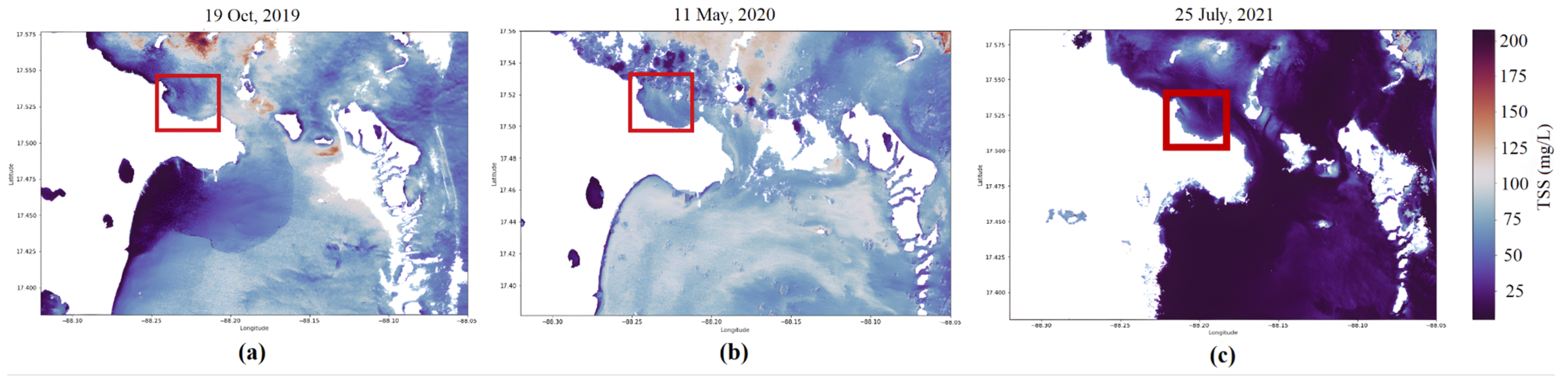
2.3.3. Time-Series Analysis

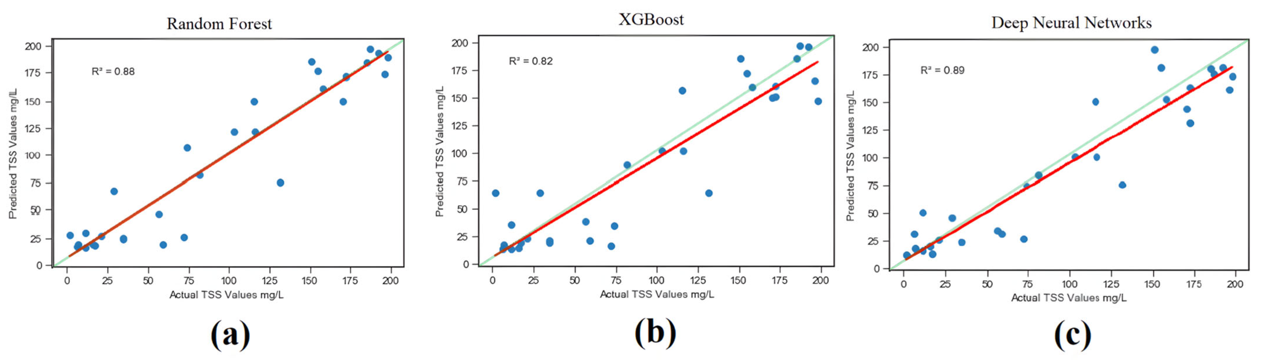
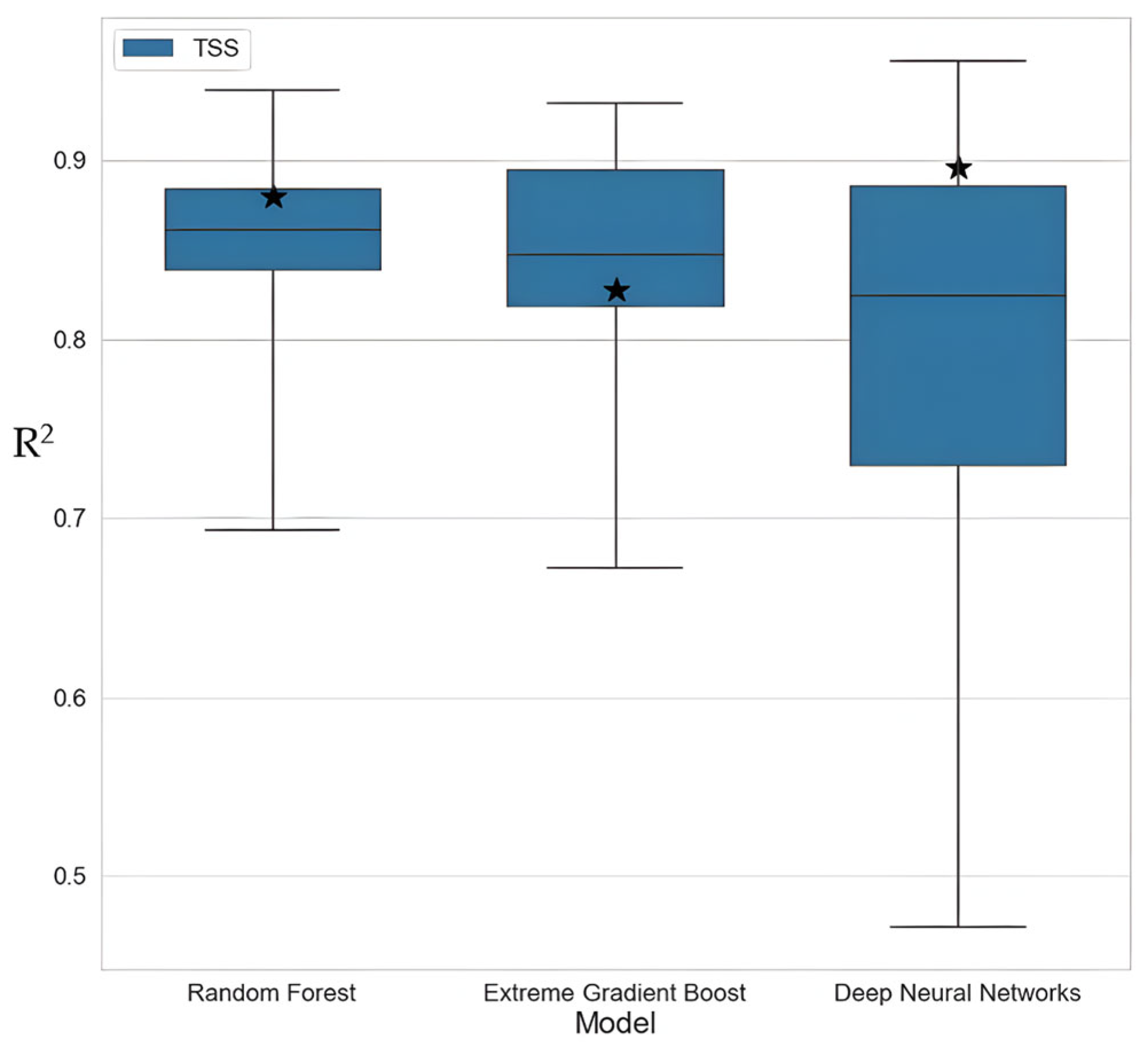
Apart from using ML models to estimate TSS concentration in the BCL, this study also focused on analyzing the changing trends of TSS in the BCL spatio-temporally. These trends were then cross-analyzed with other TSS-related bio-physical trends, such as precipitation, and were also decomposed using the Bayesian Changepoint Detection (BCD) method [60] to isolate timestamps and events having anomalous TSS concentrations. BCD works by identifying the timesteps where one of the inherent quantity parameters (viz mean value) changes, causing an outlier deviating significantly from the distribution.

BCL experiences a heavy wet season (May to November), and TSS levels are significantly driven by precipitation, apart from agricultural and urban runoff [47]. Therefore, the TSS concentration time-series plots were compared to the precipitation events between 2015 and 2021. The NASA MERRA 2.0 model was used to derive monthly time-averaged precipitation data from 2015 to 2021. The time-series plots were also compared to the diffuse attenuation coefficient at 490 nm (K_d 490), which is used as a water-clarity-based water quality indicator [34]. K_d (490) is a level-2 product that merges activity between SeaWiFs, MODIS, and MERIS instruments. K_d (490) data used for this research are a daily average of the Central Belize region. Key revelations of the time-series analysis linked the anomalous TSS timestamps with potential dredging events taking place in Belize. We discuss the analyses of these trends in detail in the discussion section.

3. Results

We only present the results of ML model training here. Since the time-series analyses of TSS concentrations are heavily tied with the subsequent discussions, we present them in the discussion section to maintain better flow. Each of the three ML algorithms for satellite-based TSS retrieval was validated using corresponding in situ field TSS concentration for each fold of training. Metrics such as MSE (Equation (2)) and coefficient of determination (R²) (Equation (3)) were used to evaluate the overall performance of the models. MSE quantifies the statistical error between a predicted TSS value against its corresponding actual value. R² explains the variation in the dependent variable (TSS) based on the independent variables (covariables discussed in Section 2.3.1), indicating the strength of the model based on that set of covariables. These metrics are commonly used not only in evaluating ML models but also for enhancing model performance [10].

Table 4. Performance metrics of the three ML algorithms—RF, XGB, and DNN for TSS estimation on training and testing sets, respectively, after 10-fold cross-validation.

	Training Set		Testing Set
Model	R2	MSE	R2	MSE
RF	0.87	0.011	0.88	0.014
XGBoost	0.85	0.015	0.82	0.0211
DNN	0.83	0.027	0.89	0.0127

shows the overall evaluation metrics of TSS estimation for all three ML algorithms. Figure 2 further shows test prediction fit plots for each algorithm.

All three algorithms achieved an R² of over 0.8 for both training and testing sets. The DNN algorithm, however, had the highest testing R² of 90% and the lowest testing MSE of 0.013 among all three algorithms. The prediction fit line is shown in red, and the reference (1:1) line is shown in green. Based on the fit lines and reference lines in Figure 2, it can be noted that RF did not show any systematic underestimation or overestimation. XGBoost and DNN, on the other hand, do show signs of systematic underestimation for higher values of TSS, roughly ranging from 125 mg/L to 200 mg/L. The same can be inferred from the box plots of R² values of the three models shown in Figure 3. The box plot for XGBoost shows a median skew in its interquartile range (IQR) of testing R2, indicating more predictions having a lower R2. The box plot for RF is the narrowest, indicating the variance agreement in general for the predicted values, in contrast with that of DNN, which is the widest, indicating high variance in general in its predictions. This contributes to DNN having a higher R² (indicated by the star on the plot and the wide IQR) than the other two models. DNN-predicted TSS values have the smallest residuals and, hence, the smallest MSE. Since the dataset is small (n = 203), we also consider the IQR of testing R2, apart from the training and testing metrics in general. This makes DNN the best-performing ML algorithm for TSS among the three, based on its wider testing R2 IQR as well as training and testing MSE. The range of sampled TSS started from as low as 8 mg/L and went up to 200 mg/L. The DNN model was also used to predict TSS concentrations for the same region for the last five years to gap-fill the TSS time-series trends discussed in the upcoming sections. Overall, the predicted TSS concentrations ranged from 5 mg/L to 150 mg/L.

Figure 4 shows the spatio-temporal maps for TSS for the entire BCL region after masking out land area and cloud cover. These maps help illustrate the underlying spatial patterns of TSS and how they change over time.

4. Discussion

4.1. Remote Sensing of TSS in BCL Using ML Algorithms

Remote sensing has been traditionally used for modeling TSS [28]. With the optically complex nature of BCL’s water ecosystem, ML algorithms can help quantify non-linear relationships more accurately than conventional methods. Choosing the right set of covariables is key for an ML algorithm to accurately model TSS. The fact that TSS can be a water clarity indicator and its concentration can impede light penetration hints at what regions of the electromagnetic spectrum may be useful for TSS modeling. Saberioon et al., 2020, used the water spectral indices mentioned in Table 3 as covariables in estimating Chl-a and TSS and reported that TSS concentrations were highly correlated with spectral indices that consisted of a combination of Vis, NIR, and Short-Wave Infrared (SWIR) channels [50]. Gernez et al. (2015) found a linear relationship between suspended particles and the NIR/Vis reflectance in the turbid waters of the Loire estuary, where the concentration range was relatively wider (10–500 mg/L) [51]. They also stated that this linear relationship was enough to estimate the suspended particle concentration. Caballero et al. (2018) further found that water spectral indices consisting of Vis and NIR channels had higher sensitivity to TSS concentrations [52].

4.2. Time-Series Analysis of TSS Concentration Trends in Central Belize

To better understand the TSS levels and their spatio-temporal variation in the BCL, we plotted monthly TSS and precipitation trends from 2015 to 2021 for various locations in the Central Belize region. These time-series trends are a combination of in situ TSS concentrations and predicted TSS concentrations, equally spaced at two weeks. Each point is a weighted median calculated from 10 readings spanning across 14 days. This is done to account for the dynamic and constantly rapidly changing nature of TSS. Corresponding precipitation data are extrapolated from monthly frequency to bi-monthly frequency in order to match the TSS trend frequency. We holistically present the TSS concentration time-series analyses results in this section, entwined with discussions for improved flow. The sampling locations for these time-series plots were in Haulover Creek, the Belize River mangrove region, and the Belize coast, all within the Central Belize region (Figure 5).

The wet season in Belize spans from May to November, and precipitation events cause runoff from nearby agricultural and urban areas into coastal waters, thus increasing the TSS [47]. Therefore, the time-series plots were compared to the precipitation events between 2015 and 2021. A lag of ~1 month may appear between the precipitation events and the peaks in TSS concentrations in these time series. This can be attributed to the tropical climate of Belize influencing a higher baseline of TSS and the difference in temporal resolution of the TSS and precipitation trends. We used the K_d (490) as a daily average of the Central Belize region (Figure 5) extrapolated to match spatially and temporally the TSS trend. We have TSS field samples from Haulover Creek (Figure 5b) and the Belize River (Figure 5d), which are confined and more influenced by activities occurring locally in Belize City. We have samples from the Belize coastal region, as well (Figure 5c), which represent the intermixing of river water and coastal water. Stations NA14, NA15, NA16, NA17, and NA18 represent in situ TSS data from Haulover Creek. Stations NA26, NA27, NA28, NA29, and NA50 represent in situ TSS data from the Belize River, while stations NA01, NA02, NA03, NA04 NA05, NA06, NA07, NA08, NA10, and NA11 represent in situ TSS data from the Belize coastal region. Intermittent dredging events become more evident in spatial and temporal analyses of TSS for the three study regions in the form of anomalous crests in the TSS trend. We used BCD-based time-series analyses [60] to discuss the potential of satellite-based TSS estimation to map and detect these dredging events in time as anomalous TSS hotspots.

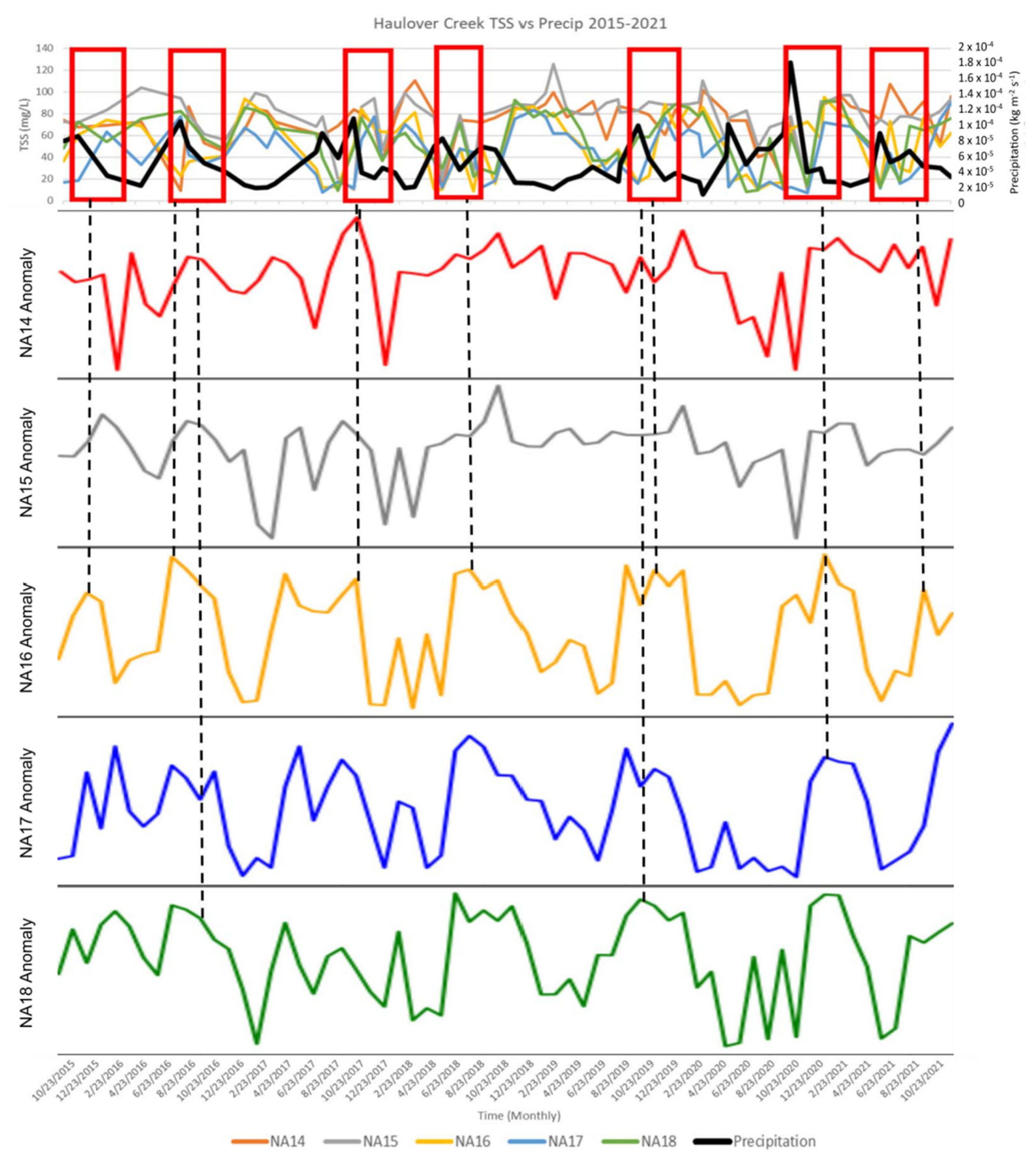
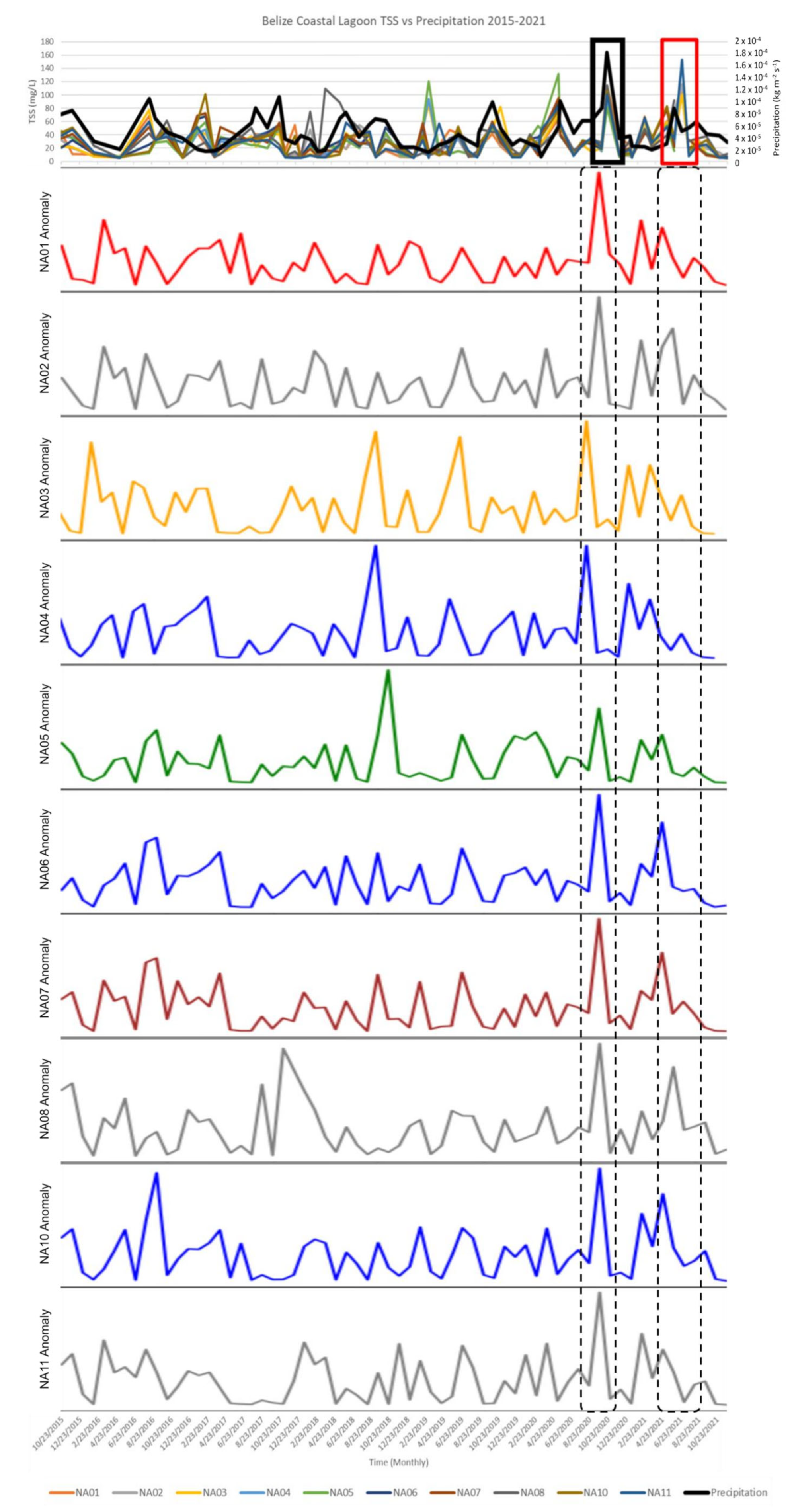
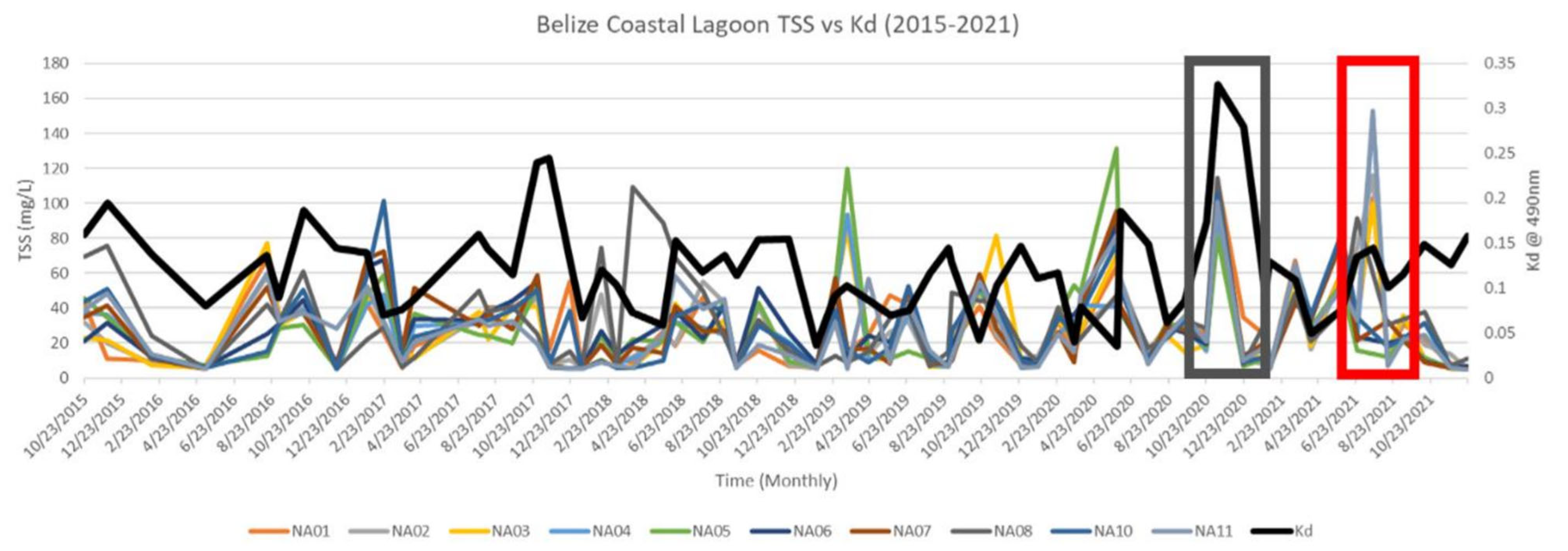
4.2.1. Haulover Creek and Belize Coastal Region Time-Series Analysis

It is essential to note that this region of Haulover Creek passes through the middle of Belize City and experiences high boat traffic and sewage disposal from nearby communities. Marine traffic causes turbulence due to boats’ propellers and movements, and this disturbs sediments, resulting in sediment resuspension in the water column, effectively increasing TSS concentrations [47,61]. In addition, precipitation events trigger runoff from surrounding communities and an increase in the creek’s streamflow. Increased runoff and streamflow combined with resuspension activity due to boat traffic can be attributed to elevated TSS levels in these sampling locations. Figure 5a shows the sampling locations from Haulover Creek. Figure 6 shows the TSS time series from the Haulover Creek stations along with the precipitation time series. The plots show high levels of TSS (~80 mg/L) throughout the year at most of the sampling points. The time-series plots indicate that precipitation and TSS may be correlated because precipitation events were usually followed by elevated levels of TSS. In Figure 6, the red boxes highlight precipitation events followed by TSS peaks. We reinforce the identification of the TSS peaks by applying BCD for decomposing the TSS time-series of each station. BCD assigns an anomaly score to each instance of a trend, creating an anomaly trend for every TSS trend. The timestamps that receive the highest anomaly score are identified as anomalous events, which in this case would be anomalously high TSS concentrations. Figure 6 shows the anomaly trend for each station and the corresponding red boxes on the TSS and precipitation trends. It should be noted that there is a lag of approximately a month between the precipitation event and the increase in TSS concentration.

The region where Haulover Creek opens out to the Belize lagoon is a highly active zone for boats accessing Belize City Port. Figure 5c shows the sampling locations from the BCL where the Belize City Port is located. These figures depict the TSS concentrations from 2015 to 2021 compared with K_d (490) and precipitation events. In Figure 7, we see that precipitation does play a role in controlling TSS concentrations because elevated TSS can be directly correlated to a precipitation event. Therefore, a seasonal pattern of TSS in the BCL can be attributed to the wet season of Belize. Figure 4a–c depicts spatial distribution maps of TSS from 19 October 2019 and 11 May 2020 and shows elevated levels of TSS in the BCL region highlighted by a red box (Figure 4c), further proving the seasonal pattern between precipitation and TSS levels. However, as mentioned above, this area is an active zone for boats as it is the main mouth of the Belize River, used by tourists and coast guards, leading to constant resuspension activities. Resuspension does not allow sediments to settle to the bottom, leading to elevated TSS levels frequently throughout the year. High K_d values are correlated with a decrease in water clarity, and from September through October, there were severe hurricane events in the Caribbean. Hurricane Nana, Hurricane Cristbol, and Hurricane Amanda occurred during this season of 2020 [34]. These events led to elevated TSS levels in November and increased turbidity in this region, showing high K_d values in that month. In November 2020, TSS concentration, precipitation, and K_d (490) all peaked anomalously as an aftermath of the hurricane season. Figure 8 shows the anomalous K_d (490) peak highlighted by the dark gray box. The peak in precipitation and TSS are shown in Figure 7, highlighted by the black box.

When overlaying the TSS trend along with the K_d trend (Figure 8), there is a peak in TSS levels in July 2021 (highlighted in the red box). This is due to a dredging event that took place in the Belize City Port from 22 June 2021 to 30 September 2021. Dredging events can expel large amounts of suspended sediments, and this elevated peak of TSS (~150 mg/L) and K_d can be attributed directly to the dredging activity. This peak is also shown in the TSS concentration trend in Figure 7, highlighted by a red box.

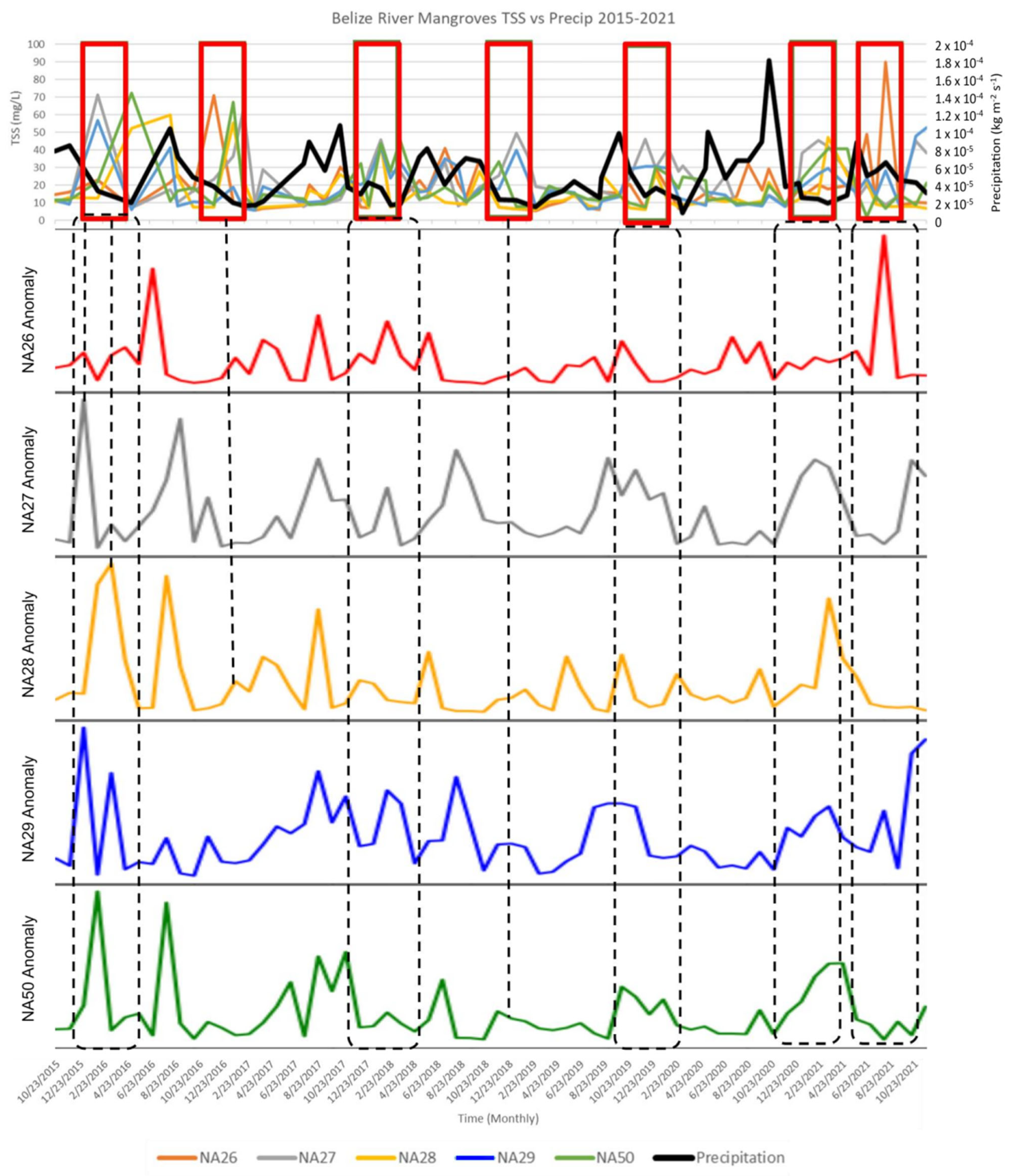
4.2.2. Belize River Time-Series Analysis

Figure 9 shows the TSS time series from 2015 to 2021 for the sampling locations from the mangrove region in the Belize River (Figure 5d). This region of the Belize River is dominated by urban development and contributes to TSS levels in the river through runoff triggered by precipitation events. This region of the Belize River also experiences lower streamflow, allowing the suspended sediments to settle to the bottom [62]. In Figure 9, the areas highlighted by the red boxes show a pattern of elevated TSS levels. This pattern is highlighted because this area generally seems to experience a lag in increased TSS levels that can be attributed to precipitation events from a month before (for every year). For example, in Figure 4c, which shows the spatial distribution map from 25 July 2021, we see elevated levels of TSS near the Belize River mangrove sampling locations (areas highlighted with the dark red box in Figure 4c) that may be attributed to high precipitation from June 2021.

4.3. Water Quality in Belize Coastal Lagoon (BCL)—Towards Sustainable Development Goals

The United Nations’ Sustainable Development Goals (SDGs) address the conservation and sustainable use of oceans and forests, highlighting the importance of protecting marine resources (United Nations (UN), 2018). Due to climate change, oceans are under severe threat. Increasing marine pollution, warming oceans, ocean acidification, and eutrophication events are all factors affecting the health of the world’s marine ecosystems and are resulting in the unsustainable use of resources provided by the ocean. According to the 2021 SDG report by the United Nations, SDG 14 encourages the “conservation and sustainable use of the ocean, seas, and marine resources for the sustainable development by protecting life underwater” and explicitly focuses on combating the issues previously mentioned. Target 14.5, specifically, aims at the “conservation of at least 10% of coastal and marine areas”, and Belize has successfully fulfilled this goal. However, further efforts are needed to fulfill the remaining SDG goals. This research aims to support Belize in successfully meeting and managing SDG 14 while addressing the challenges posed by climate change and unsustainable resource use.

The BCL’s water quality is mainly influenced by its TSS concentrations, which can be attributed to factors such as runoff, pollution, resuspension, weather, and water flow [63]. Belize’s economy thrives on commercial fishing and eco-tourism, housing several cargo ships and fishing boats in its shallow-water ports and canals. The year 2022 saw over 240,000 tourists and approximately 615,000 cruise ship visitors [64,65]. However, cruise ships have been identified as a significant source of pollution in the Caribbean, generating an average of 2228 gallons of oily bilge water and 1 metric ton of garbage daily [65]. The volume of cruise ship tourism in Belize increased by 15.9% just in the past year, contributing to rapid coastal development activities [65,66]. While this growth has positive economic impacts, it often leads to poorly managed coastal development, posing a threat to marine habitats [65,67].

Coastal development activities, such as dredging, have detrimental effects on submerged habitats, reefs, mangroves, and seagrass [65,67]. Dredging projects near the Belize Barrier Reef (BBR) have become common due to the proximity of the port, posing risks to coastal communities and natural resources [65]. Dredging often releases sediments from deeper layers that contain different mineralogies and compositions compared to sediments near the reef systems [67,68,69]. Sediment loads raised by dredging can contain unwanted contaminants [70] and can cause acidification, eutrophication, and significant harm to coral reefs [15,19,23,67].

Furthermore, population growth and urbanization near the coast result in increased discharge of sewage water and agricultural runoff, elevating nutrient loads in the coastal environment [71]. Over the past few decades, nutrient loads entering coastal environments have increased due to increasing human activities [72]. The agricultural runoff draining into the Mesoamerican Barrier Reef system has contributed to an increase in sediments and pollutants from fertilizers and pesticide applications [65]. Excessive nitrogen from fertilizers can lead to harmful algae blooms, eutrophication, and hypoxia, adversely impacting food webs, biodiversity, and habitat health [72]. Agricultural expansion and infrastructure needs in Belize have contributed to the loss of forest cover and an increase in the amounts of eroded sediments reaching the coastal system, especially during hurricane seasons [73,74].

Extreme weather events in Belize, such as tropical storms, hurricanes, and wildfires, have caused flooding, forest damage, and algal blooms, emphasizing the connection between land-based activities and water quality in the Belize Barrier Reef system [4,73]. In 2010, Belize was impacted by four tropical storms and a hurricane that led to major flooding events and caused significant damage to the forests [4]. In 2011, Belize faced an intense dry season that led to wildfires in Central Belize that lasted for two months [4]. Recently, in 2020, Belize faced an intense summer that led to wildfires mainly related to agricultural landscapes [75]. Typically, the aftermath of wildfires can be devastating to coastal environments like the BCL and can potentially cause algal blooms caused by sudden input of ash and nutrients pulled in by consequent monsoons [4].

4.4. Effectiveness of TSS Monitoring in BCL, Limitations and Future Scope

The TSS patterns in the time-series plots shown in Figure 6, Figure 7, Figure 8 and Figure 9 follow trends in other studies from the BBRS [34]. For instance, in 2021, a study was conducted by Callejas et al. [34] to examine the changes in water quality due to the COVID-19 lockdown in Belize using K_d (490) to measure water clarity. The COVID-19 lockdown in Belize started in March 2020, and the country started reopening its borders for travel in October 2020. Following the March 2020 lockdown, the K_d (490) was lower compared to the average K_d (490) for 2002–2019 [34]. The TSS time-series plots show the same pattern as the Kd (490) (Figure 8), where the TSS concentrations were lower in the months following the March 2020 lockdown compared to the previous years. Being able to validate the TSS retrieval model with the K_d (490) study speaks to the effectiveness of the prediction model.

It is important to note the errors and uncertainties associated with the modeling presented in this study. For instance, all ML models significantly underestimate lower TSS concentrations (<50 mg/L). The small size of the dataset warranted the use of k-fold cross-validation, which can limit the scope of scaling the models. With the reported MSEs, applying the DNN model to predict TSS at a different geographic or tropic location can also be challenging. Future work can include building a more populous dataset across a wider TSS concentration range and collecting more field and satellite co-incident data points to improve overall TSS modeling.

5. Conclusions

The DNN algorithm had the lowest test MSE (0.0127) and highest R² (0.89) compared to RF and XGBoost algorithms. Combining machine learning algorithms with satellite data can help us observe and understand TSS distribution in the BBRS. The time-series plots assist in identifying patterns of TSS due to factors such as weather patterns, locations of sampling sites, water flow, and anthropogenic activities. We hypothesized that pollution in the BBRS has increased significantly due to increased tourism and urban development. Data retrieved by the TSS estimation model show us that the areas in the Belize River and the coast dominated by urban activities frequently experience elevated levels of suspended sediments. The results of this study can support the claims that land-based activities affect the water quality in the BBRS. The correlation between the model findings and the K_d(490) patterns promotes confidence in the model’s ability as a forecasting tool to predict seasonal patterns and how future anthropogenic and LULC changes might affect the water quality in Belize. Accurate spatio-temporal monitoring and estimation of TSS concentrations and nutrient levels, using robust methods such as the one presented in this study, are crucial to understanding the drivers of TSS and water quality. Moreover, such methods can contribute to the sustainable management of coral reefs and water quality in Belize’s coastal ecosystems and advance fulfilling the remaining SDG goals.

References

1. Waight, K.; Ake, J.; Romero, J.; Thiagarajan, T. A Preliminary Study of Water Quality in Rural Belize. J. Microbiol. Res. 2015, 5, 41–45. [Google Scholar]
2. WRI. WRI Annual Report 2009; WRI: Washington, DC, USA, 2010. [Google Scholar]
3. Lee, M.D.; Stednick, J.D.; Gilbert, D.M. Environmental Water Quality Monitoring Program: Final Report and Annexes; For Belize Department of Environment by NARMAP, United States Agency for International Development: Belize City, Belize, 1995; 172p. [Google Scholar]
4. Azueta, J.; Enriquez-Hernández, G.; García-Flores, F.; Torres-Rodríguez, V.; Libertad, A.; Cisneros, G. State of the Belize Coastal Zone Report 2014–2018; Coastal Zone Management Authority and Institute: Belize City, Belize, 2020. [Google Scholar]
5. Wear, S.L.; Thurber, R.V. Sewage Pollution: Mitigation Is Key for Coral Reef Stewardship. Ann. N. Y. Acad. Sci. 2015, 1355, 15–30. [Google Scholar] [CrossRef] [PubMed]
6. Fisher, R.; O’Leary, R.A.; Low-Choy, S.; Mengersen, K.; Knowlton, N.; Brainard, R.E.; Caley, M.J. Species Richness on Coral Reefs and the Pursuit of Convergent Global Estimates. Curr. Biol. 2015, 25, 500–505. [Google Scholar] [CrossRef] [PubMed]
7. Balasubramanian, S.V.; Pahlevan, N.; Smith, B.; Binding, C.; Schalles, J.; Loisel, H.; Gurlin, D.; Greb, S.; Alikas, K.; Randla, M.; et al. Robust Algorithm for Estimating Total Suspended Solids (TSS) in Inland and Nearshore Coastal Waters. Remote Sens. Environ. 2020, 246, 111768. [Google Scholar] [CrossRef]
8. Miller, R.L.; McKee, B.A. Using MODIS Terra 250 m Imagery to Map Concentrations of Total Suspended Matter in Coastal Waters. Remote Sens. Environ. 2004, 93, 259–266. [Google Scholar] [CrossRef]
9. Turner, A.; Millward, G.E. Suspended Particles: Their Role in Estuarine Biogeochemical Cycles. Estuar. Coast. Shelf Sci. 2002, 55, 857–883. [Google Scholar] [CrossRef]
10. Kupssinskü, L.S.; Guimarães, T.T.; De Souza, E.M.; Zanotta, D.C.; Veronez, M.R.; Gonzaga, L.; Mauad, F.F. A Method for Chlorophyll-a and Suspended Solids Prediction through Remote Sensing and Machine Learning. Sensors 2020, 20, 2125. [Google Scholar] [CrossRef]
11. Bak, R.P.M. Lethal and Sublethal Effects of Dredging on Reef Corals. Mar. Pollut. Bull. 1978, 9, 14–16. [Google Scholar] [CrossRef]
12. Dodge, R.E.; Vaisnys, J.R. Coral Populations and Growth Patterns: Responses to Sedimentation and Turbidity Associated with Dredging. J. Mar. Res. 1977, 35, 715. [Google Scholar]
13. Erftemeijer, P.L.A.; Riegl, B.; Hoeksema, B.W.; Todd, P.A. Environmental Impacts of Dredging and Other Sediment Disturbances on Corals: A Review. Mar. Pollut. Bull. 2012, 64, 1737–1765. [Google Scholar] [CrossRef]
14. Fabricius, K.E. Effects of Terrestrial Runoff on the Ecology of Corals and Coral Reefs: Review and Synthesis. Mar. Pollut. Bull. 2005, 50, 125–146. [Google Scholar] [CrossRef] [PubMed]
15. Jones, R.; Ricardo, G.F.; Negri, A.P. Effects of Sediments on the Reproductive Cycle of Corals. Mar. Pollut. Bull. 2015, 100, 13–33. [Google Scholar] [CrossRef] [PubMed]
16. Rogers, C.S. Responses of Coral Reefs and Reef Organisms to Sedimentation. Mar. Ecol. Prog. Ser. 1990, 62, 185–202. [Google Scholar] [CrossRef]
17. Bessell-Browne, P.; Negri, A.P.; Fisher, R.; Clode, P.L.; Duckworth, A.; Jones, R. Impacts of Turbidity on Corals: The Relative Importance of Light Limitation and Suspended Sediments. Mar. Pollut. Bull. 2017, 117, 161–170. [Google Scholar] [CrossRef] [PubMed]
18. Humanes, A.; Ricardo, G.F.; Willis, B.L.; Fabricius, K.E.; Negri, A.P. Cumulative Effects of Suspended Sediments, Organic Nutrients and Temperature Stress on Early Life History Stages of the Coral Acropora Tenuis. Sci. Rep. 2017, 7, 44101. [Google Scholar] [CrossRef] [PubMed]
19. Riegl, B. Effects of Sand Deposition on Scleractinian and Alcyonacean Corals. Mar. Biol. 1995, 121, 517–526. [Google Scholar] [CrossRef]
20. Stafford-Smith, M.G.; Ormond, R.F.G. Sediment-Rejection Mechanisms of 42 Species of Australian Scleractinian Corals. Mar. Freshw. Res. 1992, 43, 683–705. [Google Scholar] [CrossRef]
21. Edmunds, P.J.; Davies, P.S. An Energy Budget for Porites Porites (Scleractinia), Growing in a Stressed Environment. Coral Reefs 1989, 8, 37–43. [Google Scholar] [CrossRef]
22. Junjie, R.K.; Browne, N.K.; Erftemeijer, P.L.A.; Todd, P.A. Impacts of Sediments on Coral Energetics: Partitioning the Effects of Turbidity and Settling Particles. PLoS ONE 2014, 9, e107195. [Google Scholar] [CrossRef]
23. Flores, F.; Hoogenboom, M.O.; Smith, L.D.; Cooper, T.F.; Abrego, D.; Negri, A.P. Chronic Exposure of Corals to Fine Sediments: Lethal and Sub-Lethal Impacts. PLoS ONE 2012, 7, e37795. [Google Scholar] [CrossRef]
24. Lirman, D.; Orlando, B.; Maciá, S.; Manzello, D.; Kaufman, L.; Biber, P.; Jones, T. Coral Communities of Biscayne Bay, Florida and Adjacent Offshore Areas: Diversity, Abundance, Distribution, and Environmental Correlates. Aquat. Conserv. 2003, 13, 121–135. [Google Scholar] [CrossRef]
25. Miller, M.W.; Karazsia, J.; Groves, C.E.; Griffin, S.; Moore, T.; Wilber, P.; Gregg, K. Detecting Sedimentation Impacts to Coral Reefs Resulting from Dredging the Port of Miami, Florida USA. PeerJ 2016, 4, e2711. [Google Scholar] [CrossRef] [PubMed]
26. Moeller, M.; Nietzer, S.; Schils, T.; Schupp, P.J. Low Sediment Loads Affect Survival of Coral Recruits: The First Weeks Are Crucial. Coral Reefs 2017, 36, 39–49. [Google Scholar] [CrossRef]
27. Ouillon, S.; Douillet, P.; Andréfouët, S. Coupling Satellite Data with in Situ Measurements and Numerical Modeling to Study Fine Suspended-Sediment Transport: A Study for the Lagoon of New Caledonia. Coral Reefs 2004, 23, 109–122. [Google Scholar]
28. Kumar, A.; Md Equeenuddin, S.; Mishra, D.R.; Acharya, B.C.; Kumar, A.; Equeenuddin, S.M.; Mishra, D.R.; Acharya, B.C. Remote Monitoring of Sediment Dynamics in a Coastal Lagoon: Long-Term Spatio-Temporal Variability of Suspended Sediment in Chilika. ECSS 2016, 170, 155–172. [Google Scholar] [CrossRef]
29. Ondrusek, M.; Stengel, E.; Kinkade, C.S.; Vogel, R.L.; Keegstra, P.; Hunter, C.; Kim, C. The Development of a New Optical Total Suspended Matter Algorithm for the Chesapeake Bay. Remote Sens. Environ. 2012, 119, 243–254. [Google Scholar] [CrossRef]
30. Feng, L.; Hu, C.; Chen, X.; Song, Q. Influence of the Three Gorges Dam on Total Suspended Matters in the Yangtze Estuary and Its Adjacent Coastal Waters: Observations from MODIS. Remote Sens. Environ. 2014, 140, 779–788. [Google Scholar] [CrossRef]
31. Luo, Y.; Doxaran, D.; Ruddick, K.; Shen, F.; Gentili, B.; Yan, L.; Huang, H.; Gordon, H.R.; Brown, O.B.; Evans, R.H.; et al. Saturation of Water Reflectance in Extremely Turbid Media Based on Field Measurements, Satellite Data and Bio-Optical Modelling. Opt. Express 2018, 26, 10435–10451. [Google Scholar] [CrossRef]
32. Ritchie, J.C.; Zimba, P.V.; Everitt, J.H. Remote Sensing Techniques to Assess Water Quality. Photogramm. Eng. Remote Sens. 2003, 69, 695–704. [Google Scholar] [CrossRef]
33. Shi, W.; Wang, M. An Assessment of the Black Ocean Pixel Assumption for MODIS SWIR Bands. Remote Sens. Environ. 2009, 113, 1587–1597. [Google Scholar] [CrossRef]
34. Callejas, I.A.; Lee, C.M.; Mishra, D.R.; Felgate, S.L.; Evans, C.; Carrias, A.; Rosado, A.; Griffin, R.; Cherrington, E.A.; Ayad, M.; et al. Effect of COVID-19 Anthropause on Water Clarity in the Belize Coastal Lagoon. Front. Mar. Sci. 2021, 8, 490. [Google Scholar]
35. Lapointe, B.E.; Tewfik, A.; Phillips, M. Macroalgae Reveal Nitrogen Enrichment and Elevated N:P Ratios on the Belize Barrier Reef. Mar. Pollut. Bull. 2021, 171, 112686. [Google Scholar] [CrossRef] [PubMed]
36. Toming, K.; Kutser, T.; Laas, A.; Sepp, M.; Paavel, B.; Nõges, T. First Experiences in Mapping Lakewater Quality Parameters with Sentinel-2 MSI Imagery. Remote Sens. 2016, 8, 640. [Google Scholar] [CrossRef]
37. Grendaitė, D.; Stonevičius, E.; Karosienė, J.; Savadova, K.; Kasperovičienė, J. Chlorophyll-a Concentration Retrieval in Eutrophic Lakes in Lithuania from Sentinel-2 Data. Geol. Geogr. 2018, 4, 15–28. [Google Scholar] [CrossRef]
38. Vanhellemont, Q.; Ruddick, K. Atmospheric Correction of Metre-Scale Optical Satellite Data for Inland and Coastal Water Applications. Remote Sens. Environ. 2018, 216, 586–597. [Google Scholar] [CrossRef]
39. Kirk, J.T.O. Light and Photosynthesis in Aquatic Ecosystems; Cambridge University Press: Cambridge, UK, 1994. [Google Scholar] [CrossRef]
40. Gao, B.C. NDWI—A Normalized Difference Water Index for Remote Sensing of Vegetation Liquid Water from Space. Remote Sens. Environ. 1996, 58, 257–266. [Google Scholar] [CrossRef]
41. Xu, H. Modification of Normalised Difference Water Index (NDWI) to Enhance Open Water Features in Remotely Sensed Imagery. Int. J. Remote Sens. 2007, 27, 3025–3033. [Google Scholar] [CrossRef]
42. Mukherjee, N.R.; Samuel, C. Assessment of the temporal variations of surface water bodies in and around Chennai using Landsat imagery. Indian J. Sci. Technol. 2016, 9, 1–7. [Google Scholar] [CrossRef]
43. Feyisa, G.L.; Meilby, H.; Fensholt, R.; Proud, S.R. Automated Water Extraction Index: A New Technique for Surface Water Mapping Using Landsat Imagery. Remote Sens. Environ. 2014, 140, 23–35. [Google Scholar] [CrossRef]
44. Lacaux, J.P.; Tourre, Y.M.; Vignolles, C.; Ndione, J.A.; Lafaye, M. Classification of Ponds from High-Spatial Resolution Remote Sensing: Application to Rift Valley Fever Epidemics in Senegal. Remote Sens. Environ. 2007, 106, 66–74. [Google Scholar] [CrossRef]
45. Birth, G.S.; McVey, G.R. Measuring the Color of Growing Turf with a Reflectance Spectrophotometer1. Agron. J. 1968, 60, 640–643. [Google Scholar] [CrossRef]
46. Zarco-Tejada, P.J.; Ustin, S.L. Modeling Canopy Water Content for Carbon Estimates from MODIS Data at Land EOS Validation Sites. Int. Geosci. Remote Sens. Symp. 2001, 1, 342–344. [Google Scholar] [CrossRef]
47. Gray, J.R.; Glysson, G.D.; Turcios, L.M.; Schwarz, G.E. Comparability of Suspended-Sediment Concentration and Total Suspended Solids Data. Water-Resources Investigations Report; 2000. [Google Scholar] [CrossRef]
48. Perlman, H. Sediment and Suspended Sediment. The USGS Water Science School. 2014. [Google Scholar]
49. Zhai, K.; Wu, X.; Qin, Y.; Du, P. Comparison of Surface Water Extraction Performances of Different Classic Water Indices Using OLI and TM Imageries in Different Situations. Geo-Spat. Inf. Sci. 2015, 18, 32–42. [Google Scholar] [CrossRef]
50. Saberioon, M.; Brom, J.; Nedbal, V.; Souček, P.; Císař, P. Chlorophyll-a and Total Suspended Solids Retrieval and Mapping Using Sentinel-2A and Machine Learning for Inland Waters. Ecol. Indic 2020, 113, 106236. [Google Scholar] [CrossRef]
51. Gernez, P.; Lafon, V.; Lerouxel, A.; Curti, C.; Lubac, B.; Cerisier, S.; Barillé, L. Toward Sentinel-2 High Resolution Remote Sensing of Suspended Particulate Matter in Very Turbid Waters: SPOT4 (Take5) Experiment in the Loire and Gironde Estuaries. Remote Sens. 2015, 7, 9507–9528. [Google Scholar] [CrossRef]
52. Caballero, I.; Steinmetz, F.; Navarro, G. Evaluation of the First Year of Operational Sentinel-2A Data for Retrieval of Suspended Solids in Medium- to High-Turbidity Waters. Remote Sens. 2018, 10, 982. [Google Scholar] [CrossRef]
53. Burke, L.; Sugg, Z.; Cherubin, L.; Kuchinke, C.; Paris, C.; Kool, J. Hydrologic Modeling of Watersheds Discharging Adjacent to the Mesoamerican Reef; World Resources Institute: Washington, DC, USA, 2006. [Google Scholar]
54. Lary, D.J.; Alavi, A.H.; Gandomi, A.H.; Walker, A.L. Machine Learning in Geosciences and Remote Sensing. Geosci. Front. 2016, 7, 3–10. [Google Scholar] [CrossRef]
55. Ahmad, H. Machine Learning Applications in Oceanography. Rev. Artic. Aquat. Res. 2019, 2, 161–169. [Google Scholar] [CrossRef]
56. Kramer, O. Scikit-Learn. Stud. Big Data 2016, 20, 45–53. [Google Scholar]
57. Domingos, P. A Few Useful Things to Know about Machine Learning. Commun. ACM 2012, 55, 78–87. [Google Scholar] [CrossRef]
58. Vanhellemont, Q.; Ruddick, K. Acolite for Sentinel-2: Aquatic Applications of MSI Imagery. European Space Agency. In Proceedings of the 2016 ESA Living Planet Symposium, Prague, Czech Republic, 9–13 May 2016; pp. 9–13. [Google Scholar]
59. Zuhlke, M.; Fomferra, N.; Brockmann, C.; Peters, M.; Veci, L.; Malik, J.; Regner, P. SNAP (Sentinel Application Platform) and the ESA Sentinel 3 Toolbox. In Sentinel-3 for Science Workshop; 2015; Volume 734, p. 21. [Google Scholar]
60. Zhao, K.; Hu, T.; Li, Y. Rbeast: Bayesian Change-Point Detection and Time Series Decomposition. R package version 0.2 2019, Volume 2. Available online: https://cran.r-project.org/web/packages/Rbeast/Rbeast.pdf (accessed on 16 September 2023).
61. Sagerman, J.; Hansen, J.P.; Wikström, S.A. Effects of Boat Traffic and Mooring Infrastructure on Aquatic Vegetation: A Systematic Review and Meta-Analysis. Ambio 2020, 49, 517–530. [Google Scholar] [CrossRef] [PubMed]
62. Dubon, W.F. Belize River Water Quality—A Baseline Chemical Assessment; University of Belize: Belmopan, Belize, 2013. [Google Scholar]
63. McNally, W.H.; Mehta, A.J. Sediment Transport and Deposition in Estuaries (Sample Chapter). In Encyclopedia of Life Support Systems (EOLSS): Coastal Zones and Estuaries; 2004. [Google Scholar]
64. Cruise Passenger Arrivals in Belize 2022|Statista. Available online: https://www.statista.com/statistics/387145/cruise-tourism-volume-belize/ (accessed on 14 September 2023).
65. Burke, L.; Maidens, J. Belize Coastal Threat Atlas; World Resources Institute: Washington, DC, USA, 9 January 2005. Available online: https://www.wri.org/belize-coastal-threat-atlas (accessed on 1 May 2023).
66. Statistics|Belize Tourism Board. Available online: https://www.belizetourismboard.org/belize-tourism/statistics/ (accessed on 14 September 2023).
67. Cunning, R.; Silverstein, R.N.; Barnes, B.B.; Baker, A.C. Extensive Coral Mortality and Critical Habitat Loss Following Dredging and Their Association with Remotely-Sensed Sediment Plumes. Mar. Pollut. Bull. 2019, 145, 185–199. [Google Scholar] [CrossRef] [PubMed]
68. Saussaye, L.; van Veen, E.; Rollinson, G.; Boutouil, M.; Andersen, J.; Coggan, J. Geotechnical and Mineralogical Characterisations of Marine-Dredged Sediments before and after Stabilisation to Optimise Their Use as a Road Material. Environ. Technol. 2017, 38, 3034–3046. [Google Scholar] [CrossRef] [PubMed]
69. Swart, P.K. Report on the Mineralogy and the Stable Carbon and Oxygen Isotopic Composition of Samples Supplied by NOAA. 2016. [Google Scholar]
70. Jones, R.J. Spatial Patterns of Chemical Contamination (Metals, PAHs, PCBs, PCDDs/PCDFS) in Sediments of a Non-Industrialized but Densely Populated Coral Atoll/Small Island State (Bermuda). Mar. Pollut. Bull. 2011, 62, 1362–1376. [Google Scholar] [CrossRef] [PubMed]
71. Cherrington, E.; Kay, E.; Waight-Cho, I. Modelling the Impacts of Climate Change and Land. Use Change on Belize’s Water Resources: Potential. Effects on Erosion and Runoff. 2015. [Google Scholar] [CrossRef]
72. Zhang, P.; Chen, Y.; Peng, C.; Dai, P.; Lai, J.; Zhao, L.; Zhang, J. Spatiotemporal Variation, Composition of DIN and Its Contribution to Eutrophication in Coastal Waters Adjacent to Hainan Island, China. Reg. Stud. Mar. Sci. 2020, 37, 101332. [Google Scholar] [CrossRef]
73. Cherrington, E.A.; Ek, E.; Cho, P.; Howell, B.F.; Hernandez, B.E.; Anderson, E.R.; Flores, A.I.; Garcia, B.C.; Sempris, E.; Irwin, D.E. Forest Cover and Deforestation in Belize: 1980–2010. SERVIR, 2010. [Google Scholar]
74. Belizean. Belize Country Report on the Protection of Coral Reef as It Relates to the un Secretary General Report. 2021.
75. Government’s Response to Wildfire Situation—Government of Belize Press Office. Available online: https://www.pressoffice.gov.bz/governments-response-to-wildfire-situation/ (accessed on 14 September 2023).
Figure 1. Location of sampling sites (inland and into the BBRS) depicted as red dots on a LandSat-8 image from 20 May 2019.
Remotesensing 15 05625 g001
Figure 2. Prediction fit plots for actual and predicted TSS values for (a) RF, (b) XGB, (c) DNN models for TSS estimation. The red line is the best-fit line of actual vs. predicted values, and the green line is the reference (1:1) line.
Remotesensing 15 05625 g002
Figure 3. Box plot of training R2 of all three models after cross-validation. The testing R2 value for each model is marked with a star.
Remotesensing 15 05625 g003
Figure 4. Spatio-temporal maps of TSS prepared using the DNN model for the BCL region across 3 years. The red box highlights the area where the Belize River opens up into the BCL, a transition zone between fresh and lagoon waters, and a potentially frequent dredging location. TSS levels within the red box can be seen to be anomalously high in July 2021 from among the three pictures. Only water pixels are shown; all non-water pixels (land/cloud) are masked out.
Remotesensing 15 05625 g004
Figure 5. (a) Sentinel-2 scene captured on 19 October 2019 with an opaque box highlighting the Central Belize region for where the average daily Kd (490) was calculated, (b) Inset of the Haulover Creek region with TSS field sampling locations marked with star symbols, (c) Inset of Belize coastal region with TSS field sampling locations marked with start symbols, (d) Inset of Belize River with TSS field sampling locations marked with start symbols.
Remotesensing 15 05625 g005
Figure 6. TSS concentration trend, precipitation trend, and the BCD anomaly from each station in Haulover Creek for the 2015–2021 period. The first row contains the TSS concentration trends for the NA14, NA15, NA16, NA17, and NA18 stations, as well as precipitation. The rows below the first one contain the trend decomposition of the TSS concentration trend of each station as obtained from BCD analysis, which shows the magnitude of anomalies. Anomalous TSS concentrations co-incident with anomalous precipitation events are highlighted in the red boxes. Each red box (anomalous TSS event) is drawn based on the timestamp of the TSS anomaly trend for each station derived from BCD analysis. The dominating anomaly for each flagged event (red box) is connected by a black dotted line.
Remotesensing 15 05625 g006
Figure 7. TSS concentration trend, precipitation trend, and the BCD anomaly from each station in the BCL for the 2015–2021 period. The first row contains the TSS concentration trends for the NA01, NA02, NA03, NA04, NA05, NA06, NA07, NA08, NA10, and NA11 stations, as well as precipitation. The rows below the first one contain the trend decomposition of the TSS concentration trend of each station as obtained from BCD analysis, which shows the magnitude of anomalies. Anomalous TSS concentrations co-incident with anomalous precipitation events are highlighted in the red and black boxes. Each box (anomalous TSS event) is drawn based on the timestamp of the TSS anomaly trend for each station derived from BCD analysis. The dominating anomaly for each flagged event (red and black boxes) is connected by a dashed black box, indicating the probability flag being in the temporal neighborhood of the anomalous TSS.
Remotesensing 15 05625 g007
Figure 8. TSS concentration trend overlayed with the Kd trend and the BCD anomaly from each station in the BCL for the 2015–2021 period. Anomalous TSS concentrations that followed the dredging-induced anomalous Kd are highlighted by a red box. Anomalously high Kd values in the trend are highlighted by a black box.
Remotesensing 15 05625 g008
Figure 9. TSS concentration trend, precipitation trend, and the BCD anomaly from each station in the Belize River for the 2015–2021 period. The first row contains the TSS concentration trends for the NA26, NA27, NA28, NA29, and NA50 stations, as well as precipitation. The rows below the first one contain the trend decomposition of the TSS concentration trend of each station as obtained from BCD analysis, which shows the magnitude of anomalies. Anomalous TSS concentrations co-incident with anomalous precipitation events are highlighted in the red boxes. Each red box (anomalous TSS event) is drawn based on the timestamp of the TSS anomaly trend for each station derived from BCD analysis. The dominating anomaly for each flagged event (red box) is connected by either a black dotted line if it lines up with the anomalous TSS peak or a dashed black box if the temporal flag does not directly line up with the anomalous TSS peak but is, rather, in its neighborhood.
Remotesensing 15 05625 g009