
Evaluating Feature Selection Methods and Machine Learning Algorithms for Mapping Mangrove Forests Using Optical and Synthetic Aperture Radar Data

Abstract
:
1. Introduction
2. Materials
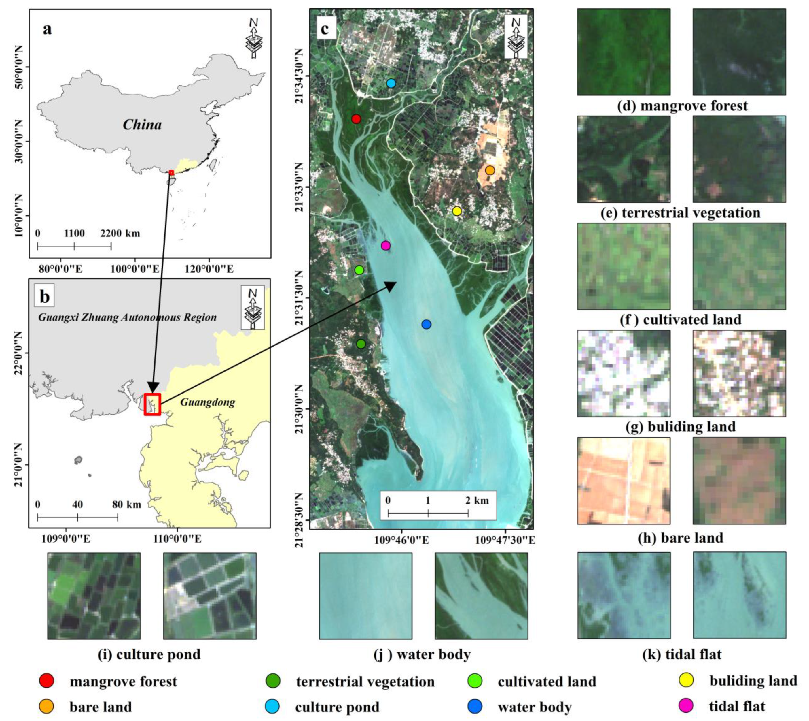
2.1. Study Area
2.2. Data
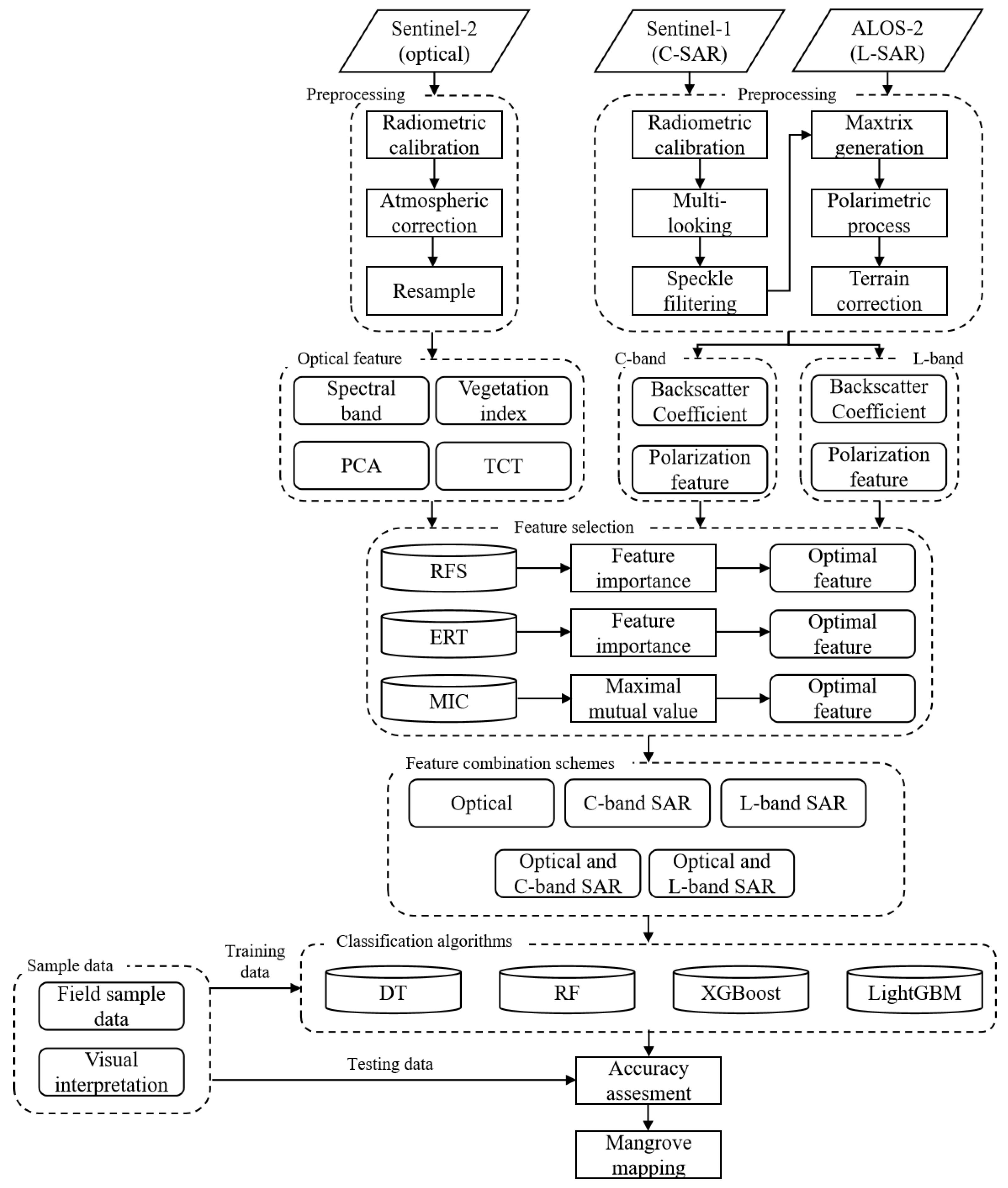
2.2.1. Satellite Data and Preprocessing
2.2.2. Sample Datasets
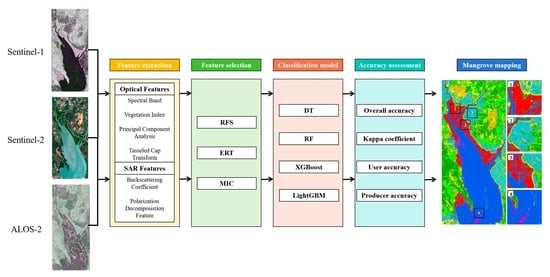
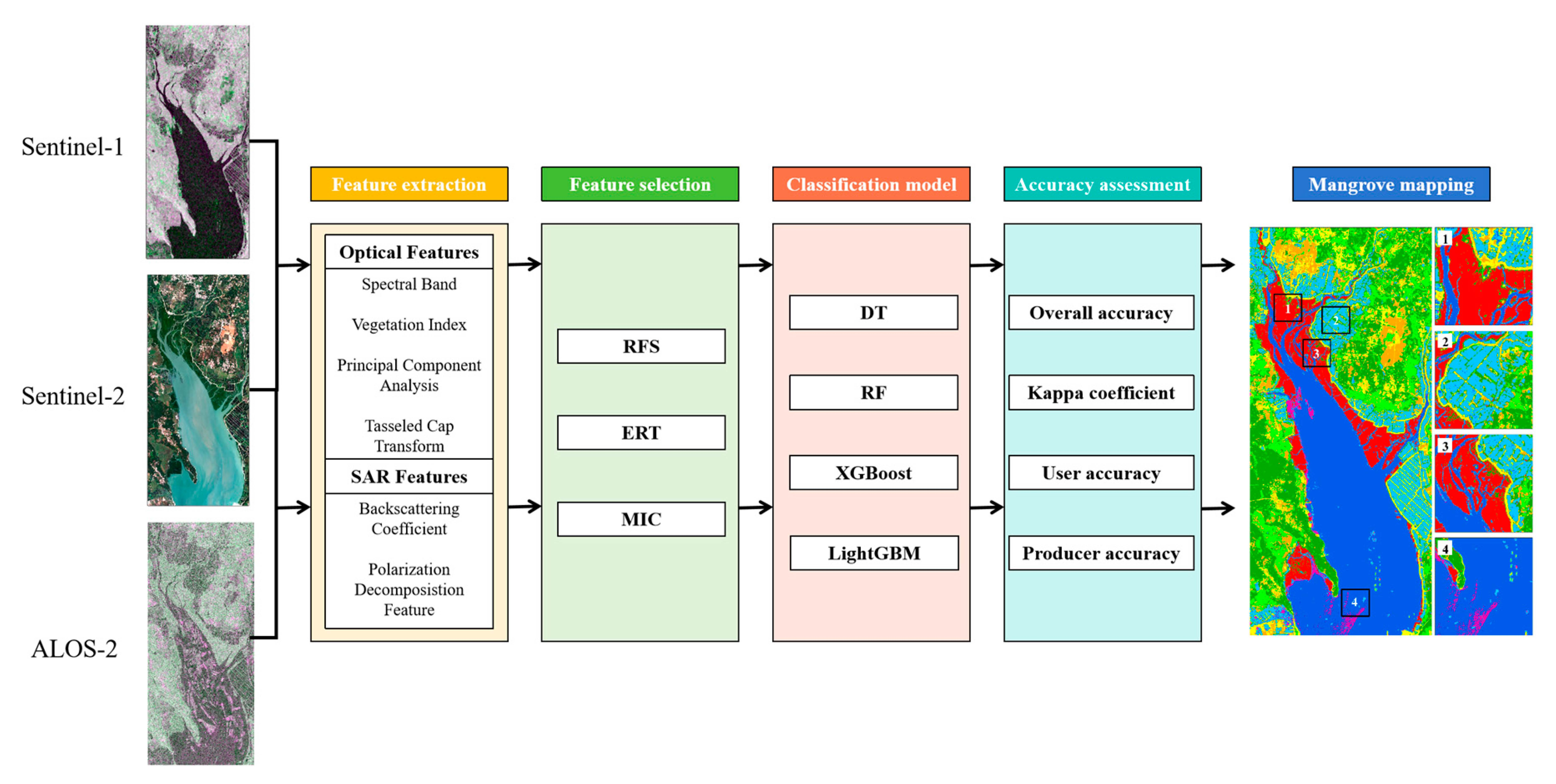
3. Methods
3.1. Feature Extraction
3.1.1. Multispectral Image Features
3.1.2. Polarimetric SAR Features
3.2. Feature Selection
3.2.1. Random Forest (RFS)
3.2.2. Extremely Randomized Tree (ERT)
3.2.3. Maximal Information Coefficient (MIC)
3.2.4. Determining the Optimal Number of Features
3.3. Image Classification with Machine Learning Algorithms
3.3.1. Decision Tree (DT)
3.3.2. Random Forest (RF)
3.3.3. Extreme Gradient Boosting (XGBoost)
3.3.4. Light Gradient-Boosting Machine (LightGBM)
3.4. Accuracy Assessment
4. Results
4.1. Classification with a Single Data Source
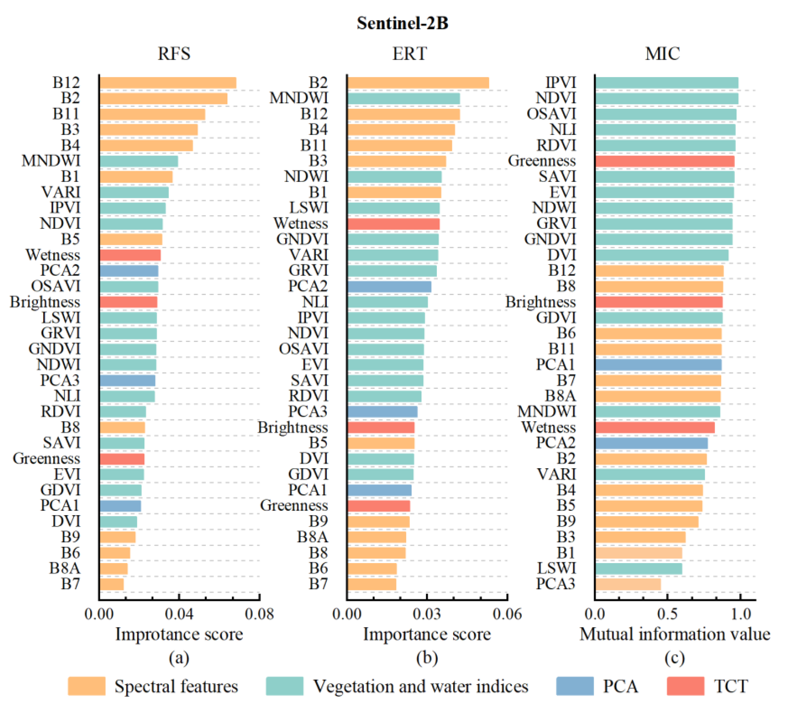
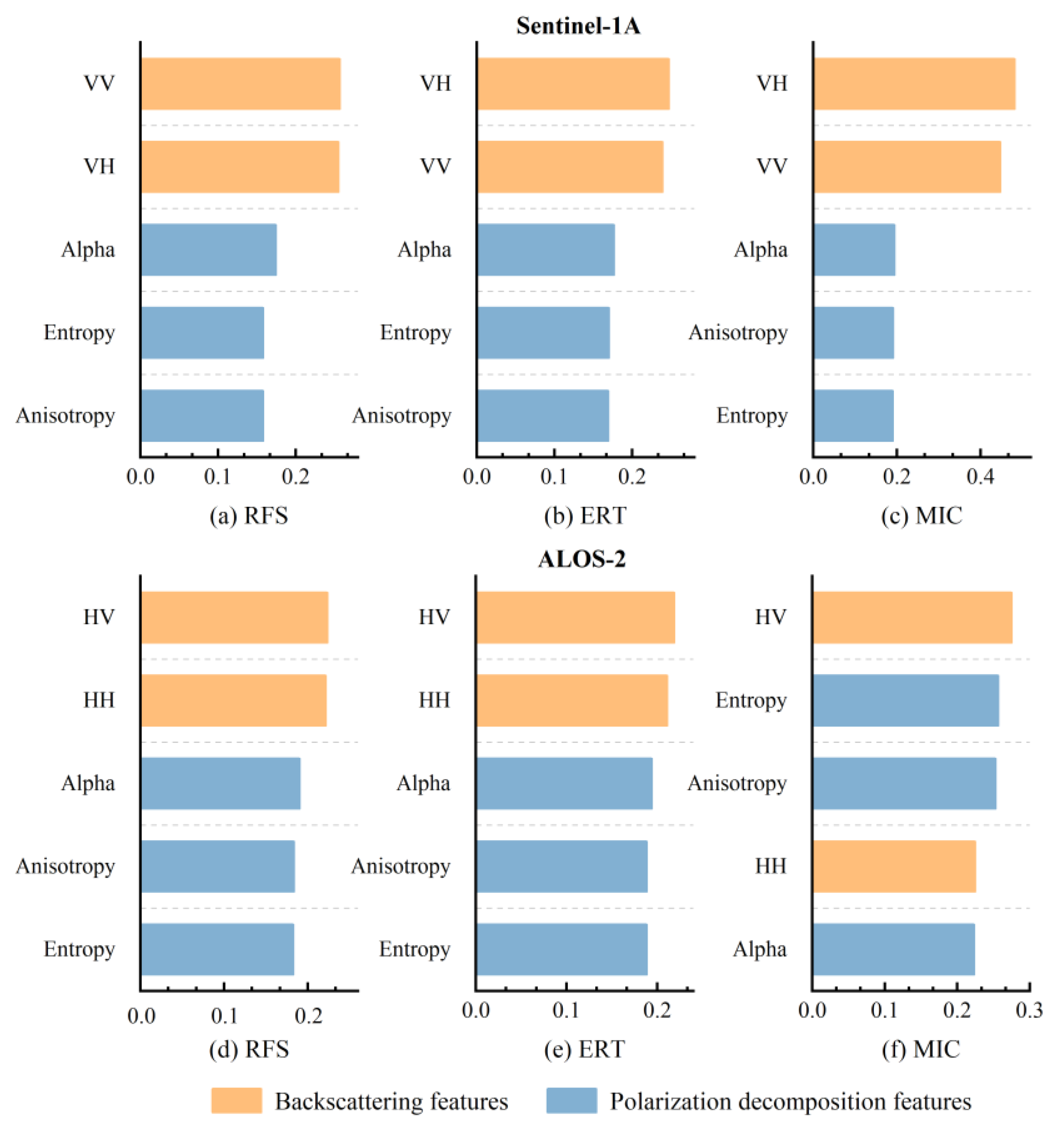
4.1.1. Feature Selection Results
4.1.2. The Accuracy of Classification for a Single Data Source
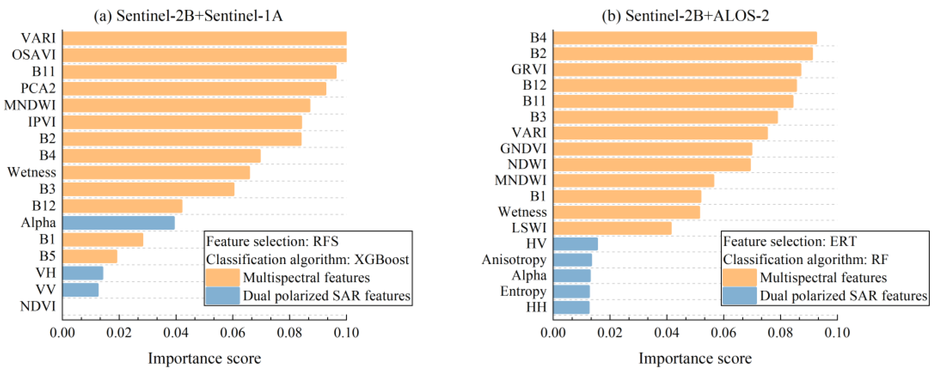
4.2. Classification with Combined Data
4.3. Comparison between C-Band and Dual-Polarized SAR and L-Band Dual-Polarized SAR
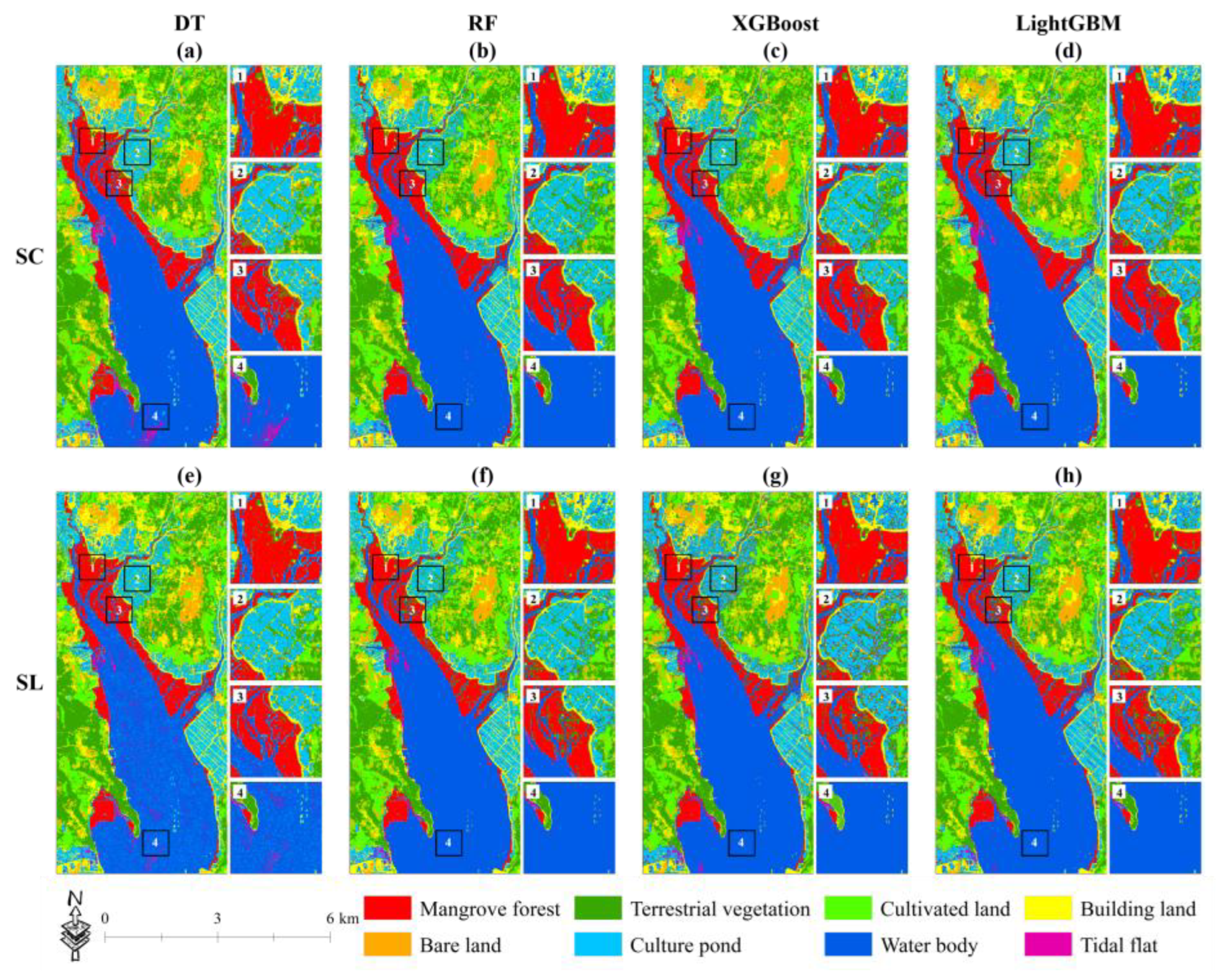
4.4. Mapping the Classification Results of Two Schemes Based on Four Machine Learning Algorithms
5. Discussion
5.1. The Contribution and Sensitive Features of Optical and SAR Images
5.2. The Impact of Different Classification Algorithms on the Classification Accuracy
5.3. Potential Application and Future Work
6. Conclusions
Author Contributions
Funding
Data Availability Statement
Conflicts of Interest
References
- Thomas, N.; Lucas, R.; Bunting, P.; Hardy, A.; Rosenqvist, A.; Simard, M. Distribution and drivers of global mangrove forest change, 1996–2010. PLoS ONE 2017, 12, e0179302. [Google Scholar] [CrossRef] [PubMed]
- Abad-Segura, E.; Gonzalez-Zamar, M.D.; Vazquez-Cano, E.; Lopez-Meneses, E. Remote Sensing Applied in Forest Management to Optimize Ecosystem Services: Advances in Research. Forests 2020, 11, 969. [Google Scholar] [CrossRef]
- Son, N.T.; Chen, C.F.; Chang, N.B.; Chen, C.R.; Chang, L.Y.; Thanh, B.X. Mangrove Mapping and Change Detection in Ca Mau Peninsula, Vietnam, Using Landsat Data and Object-Based Image Analysis. IEEE J. Sel. Top. Appl. Earth Obs. Remote Sens. 2015, 8, 503–510. [Google Scholar] [CrossRef]
- Wang, L.; Jia, M.M.; Yin, D.M.; Tian, J.Y. A review of remote sensing for mangrove forests: 1956–2018. Remote Sens. Environ. 2019, 231, 111223. [Google Scholar] [CrossRef]
- Zhao, C.P.; Qin, C.Z. 10-m-resolution mangrove maps of China derived from multi-source and multi-temporal satellite observations. ISPRS J. Photogramm. Remote Sens. 2020, 169, 389–405. [Google Scholar] [CrossRef]
- Jia, M.M.; Wang, Z.M.; Zhang, Y.Z.; Mao, D.H.; Wang, C. Monitoring loss and recovery of mangrove forests during 42 years: The achievements of mangrove conservation in China. Int. J. Appl. Earth Obs. 2018, 73, 535–545. [Google Scholar] [CrossRef]
- Jhonnerie, R.; Siregar, V.P.; Nababan, B.; Prasetyo, L.B.; Wouthuyzen, S. Random Forest Classification for Mangrove Land Cover Mapping Using Landsat 5 TM and Alos Palsar Imageries. Procedia Environ. Sci. 2015, 24, 215–221. [Google Scholar] [CrossRef]
- Ghorbanian, A.; Zaghian, S.; Asiyabi, R.M.; Amani, M.; Mohammadzadeh, A.; Jamali, S. Mangrove Ecosystem Mapping Using Sentinel-1 and Sentinel-2 Satellite Images and Random Forest Algorithm in Google Earth Engine. Remote Sens. 2021, 13, 2565. [Google Scholar] [CrossRef]
- Abdel-Hamid, A.; Dubovyk, O.; Abou El-Magd, I.; Menz, G. Mapping Mangroves Extents on the Red Sea Coastline in Egypt using Polarimetric SAR and High Resolution Optical Remote Sensing Data. Sustainability 2018, 10, 646. [Google Scholar] [CrossRef]
- Zhao, C.P.; Jia, M.M.; Wang, Z.M.; Mao, D.H.; Wang, Y.Q. Identifying mangroves through knowledge extracted from trained random forest models: An interpretable mangrove mapping approach (IMMA). ISPRS J. Photogramm. Remote Sens. 2023, 201, 209–225. [Google Scholar] [CrossRef]
- Cheng, Q.; Varshney, P.K.; Arora, M.K. Logistic regression for feature selection and soft classification of remote sensing data. IEEE Geosci. Remote Sens. Lett. 2006, 3, 491–494. [Google Scholar] [CrossRef]
- Kohavi, R.; John, G.H. Wrappers for feature subset selection. Artif. Intell. 1997, 97, 273–324. [Google Scholar] [CrossRef]
- Tang, X.H.; Wang, J.C.; Lu, J.G.; Liu, G.K.; Chen, J.D. Improving Bearing Fault Diagnosis Using Maximum Information Coefficient Based Feature Selection. Appl. Sci. 2018, 8, 2143. [Google Scholar] [CrossRef]
- Fei, H.; Fan, Z.H.; Wang, C.K.; Zhang, N.N.; Wang, T.; Chen, R.G.; Bai, T.C. Cotton Classification Method at the County Scale Based on Multi-Features and Random Forest Feature Selection Algorithm and Classifier. Remote Sens. 2022, 14, 829. [Google Scholar] [CrossRef]
- Fu, B.; Liang, Y.; Lao, Z.; Sun, X.; Li, S.; He, H.; Sun, W.; Fan, D. Quantifying scattering characteristics of mangrove species from Optuna-based optimal machine learning classification using multi-scale feature selection and SAR image time series. Int. J. Appl. Earth Obs. 2023, 122, 103446. [Google Scholar] [CrossRef]
- Held, A.; Ticehurst, C.; Lymburner, L.; Williams, N. High resolution mapping of tropical mangrove ecosystems using hyperspectral and radar remote sensing. Int. J. Remote Sens. 2003, 24, 2739–2759. [Google Scholar] [CrossRef]
- Li, W.Z.; El-Askary, H.; Qurban, M.A.; Li, J.J.; ManiKandan, K.P.; Piechota, T. Using multi-indices approach to quantify mangrove changes over the Western Arabian Gulf along Saudi Arabia coast. Ecol. Indic. 2019, 102, 734–745. [Google Scholar] [CrossRef]
- Jafarzadeh, H.; Mahdianpari, M.; Gill, E.; Mohammadimanesh, F.; Homayouni, S. Bagging and Boosting Ensemble Classifiers for Classification of Multispectral, Hyperspectral and PolSAR Data: A Comparative Evaluation. Remote Sens. 2021, 13, 4405. [Google Scholar] [CrossRef]
- Zhen, J.N.; Liao, J.J.; Shen, G.Z. Mapping Mangrove Forests of Dongzhaigang Nature Reserve in China Using Landsat 8 and Radarsat-2 Polarimetric SAR Data. Sensors 2018, 18, 4012. [Google Scholar] [CrossRef]
- Ke, G.; Meng, Q.; Finley, T.; Wang, T.; Chen, W.; Ma, W.; Ye, Q.; Liu, T.-Y. LightGBM: A Highly Efficient Gradient Boosting Decision Tree. Adv. Neurol. 2017, 30, 52. [Google Scholar]
- Miao, J.; Zhen, J.N.; Wang, J.J.; Zhao, D.M.; Jiang, X.P.; Shen, Z.; Gao, C.J.; Wu, G.F. Mapping Seasonal Leaf Nutrients of Mangrove with Sentinel-2 Images and XGBoost Method. Remote Sens. 2022, 14, 3679. [Google Scholar] [CrossRef]
- Su, H.; Lu, X.M.; Chen, Z.Q.; Zhang, H.S.; Lu, W.F.; Wu, W.T. Estimating Coastal Chlorophyll-A Concentration from Time-Series OLCI Data Based on Machine Learning. Remote Sens. 2021, 13, 576. [Google Scholar] [CrossRef]
- Fu, B.; He, X.; Yao, H.; Liang, Y.; Deng, T.; He, H.; Fan, D.; Lan, G.; He, W. Comparison of RFE-DL and stacking ensemble learning algorithms for classifying mangrove species on UAV multispectral images. Int. J. Appl. Earth Obs. 2022, 112, 102890. [Google Scholar] [CrossRef]
- Guyon, I.; Elisseeff, A. An introduction to variable and feature selection. J. Mach. Learn. Res. 2003, 3, 1157–1182. [Google Scholar]
- You, M.; Liu, J.; Li, G.-Z.; Chen, Y. Embedded Feature Selection for Multi-label Classification of Music Emotions. Int. J. Comput. Intell. Syst. 2012, 5, 668–678. [Google Scholar] [CrossRef]
- Al-Ahmadi, F.S.; Al-Hames, A.S. Comparison of four classification methods to extract land use and land cover from raw satellite images for some remote arid areas, Kingdom of Saudi Arabia. Earth Sci. 2009, 20, 24. [Google Scholar] [CrossRef]
- Foody, G.M.; Mathur, A. A relative evaluation of multiclass image classification by support vector machines. IEEE Trans. Geosci. Remote Sens. 2004, 42, 1335–1343. [Google Scholar] [CrossRef]
- Maxwell, A.E.; Warner, T.A.; Fang, F. Implementation of machine-learning classification in remote sensing: An applied review. Int. J. Remote Sens. 2018, 39, 2784–2817. [Google Scholar] [CrossRef]
- Breiman, L. Random forests. Mach. Learn. 2001, 45, 5–32. [Google Scholar] [CrossRef]
- Shami, S.; Azar, M.K.; Nilfouroushan, F.; Salimi, M.; Reshadi, M.A.M. Assessments of ground subsidence along the railway in the Kashan plain, Iran, using Sentinel-1 data and NSBAS algorithm. Int. J. Appl. Earth Obs. 2022, 112, 102898. [Google Scholar] [CrossRef]
- Yamaguchi, Y.; Umemura, M.; Kanai, D.; Miyazaki, K.; Yamada, H. ALOS-2 polarimetric SAR observation of Hokkaido- Iburi-Tobu earthquake 2018. Ieice Commun. Express 2019, 8, 26–31. [Google Scholar] [CrossRef]
- Vrigazova, B. The Proportion for Splitting Data into Training and Test Set for the Bootstrap in Classification Problems. Bus. Syst. Res. J. 2021, 12, 228–242. [Google Scholar] [CrossRef]
- Datt, B. Remote sensing of chlorophyll a, chlorophyll b, chlorophyll a+b, and total carotenoid content in eucalyptus leaves. Remote Sens. Environ. 1998, 66, 111–121. [Google Scholar] [CrossRef]
- Huete, A.R.; Liu, H.Q.; Batchily, K.; van Leeuwen, W. A comparison of vegetation indices global set of TM images for EOS-MODIS. Remote Sens. Environ. 1997, 59, 440–451. [Google Scholar] [CrossRef]
- Sakamoto, T.; Van Nguyen, N.; Kotera, A.; Ohno, H.; Ishitsuka, N.; Yokozawa, M. Detecting temporal changes in the extent of annual flooding within the Cambodia and the Vietnamese Mekong Delta from MODIS time-series imagery. Remote Sens. Environ. 2007, 109, 295–313. [Google Scholar] [CrossRef]
- Rondeaux, G.; Steven, M.; Baret, F. Optimization of soil-adjusted vegetation indices. Remote Sens. Environ. 1996, 55, 95–107. [Google Scholar] [CrossRef]
- Tucker, C.J. Red and photographic infrared linear combinations for monitoring vegetation. Remote Sens. Environ. 1979, 8, 127–150. [Google Scholar] [CrossRef]
- Sripada, R.P.; Heiniger, R.W.; White, J.G.; Meijer, A.D. Aerial color infrared photography for determining early in-season nitrogen requirements in corn. Agron. J. 2006, 98, 968–977. [Google Scholar] [CrossRef]
- Huete, A.R. A soil-adjusted vegetation index (SAVI). Remote Sens. Environ. 1988, 25, 295–309. [Google Scholar] [CrossRef]
- McFeeters, S.K. The use of the normalized difference water index (NDWI) in the delineation of open water features. Int. J. Remote Sens. 1996, 17, 1425–1432. [Google Scholar] [CrossRef]
- Xu, H.Q. Modification of normalised difference water index (NDWI) to enhance open water features in remotely sensed imagery. Int. J. Remote Sens. 2006, 27, 3025–3033. [Google Scholar] [CrossRef]
- Gitelson, A.A.; Kaufman, Y.J.; Stark, R.; Rundquist, D. Novel algorithms for remote estimation of vegetation fraction. Remote Sens. Environ. 2002, 80, 76–87. [Google Scholar] [CrossRef]
- Crippen, R.E. Calculating the vegetation index faster. Remote Sens. Environ. 1990, 34, 71–73. [Google Scholar] [CrossRef]
- Roujean, J.-L.; Breon, F.-M. Estimating PAR absorbed by vegetation from bidirectional reflectance measurements. Remote Sens. Environ. 1995, 51, 375–384. [Google Scholar] [CrossRef]
- Gao, C.; Jiang, X.; Zhen, J.; Wang, J.; Wu, G. Mangrove species classification with combination of WorldView-2 and Zhuhai-1 satellite images. Natl. Remote Sens. Bull. 2022, 26, 1155–1168. [Google Scholar] [CrossRef]
- Cloude, S.R.; Pottier, E. A review of target decomposition theorems in radar polarimetry. IEEE Trans. Geosci. Remote Sens. 1996, 34, 498–518. [Google Scholar] [CrossRef]
- Saraswat, M.; Arya, K.V. Feature selection and classification of leukocytes using random forest. Med. Biol. Eng. Comput. 2014, 52, 1041–1052. [Google Scholar] [CrossRef]
- Geurts, P.; Ernst, D.; Wehenkel, L. Extremely randomized trees. Mach. Learn. 2006, 63, 3–42. [Google Scholar] [CrossRef]
- Wu, M.H.; Lin, N.; Li, G.J.; Liu, H.L.; Li, D.L. Hyperspectral estimation of petroleum hydrocarbon content in soil using ensemble learning method and LASSO feature extraction. Environ. Pollut. Bioavailab. 2022, 34, 308–320. [Google Scholar] [CrossRef]
- Reshef, D.N.; Reshef, Y.A.; Finucane, H.K.; Grossman, S.R.; McVean, G.; Turnbaugh, P.J.; Lander, E.S.; Mitzenmacher, M.; Sabeti, P.C. Detecting Novel Associations in Large Data Sets. Science 2011, 334, 1518–1524. [Google Scholar] [CrossRef] [PubMed]
- Sun, G.L.; Li, J.B.; Dai, J.; Song, Z.C.; Lang, F. Feature selection for IoT based on maximal information coefficient. Future Gener. Comput. Syst. 2018, 89, 606–616. [Google Scholar] [CrossRef]
- Friedl, M.A.; Brodley, C.E. Decision tree classification of land cover from remotely sensed data. Remote Sens. Environ. 1997, 61, 399–409. [Google Scholar] [CrossRef]
- Chen, T.; Guestrin, C. XGBoost: A Scalable Tree Boosting System. In Proceedings of the 22nd Acm Sigkdd International Conference on Knowledge Discovery and Datamining, San Francisco, CA, USA, 13–17 August 2016; pp. 785–794. [Google Scholar]
- Aja, D.; Miyittah, M.K.; Angnuureng, D.B. Quantifying Mangrove Extent Using a Combination of Optical and Radar Images in a Wetland Complex, Western Region, Ghana. Sustainability 2022, 14, 16687. [Google Scholar] [CrossRef]
- Tsyganskaya, V.; Martinis, S.; Marzahn, P.; Ludwig, R. SAR-based detection of flooded vegetation - a review of characteristics and approaches. Int. J. Remote Sens. 2018, 39, 2255–2293. [Google Scholar] [CrossRef]
- Mandianpari, M.; Salehi, B.; Mohammadimanesh, F.; Motagh, M. Random forest wetland classification using ALOS-2 L-band, RADARSAT-2 C-band, and TerraSAR-X imagery. ISPRS J. Photogramm. Remote Sens. 2017, 130, 13–31. [Google Scholar] [CrossRef]
- Hess, L.L.; Melack, J.M.; Simonett, D.S. Radar detection of flooding beneath the forest canopy: A review. Int. J. Remote Sens. 1990, 11, 1313–1325. [Google Scholar] [CrossRef]
- Wang, X.Z.; Tan, L.L.; Fan, J.C. Performance Evaluation of Mangrove Species Classification Based on Multi-Source Remote Sensing Data Using Extremely Randomized Trees in Fucheng Town, Leizhou City, Guangdong Province. Remote Sens. 2023, 15, 1386. [Google Scholar] [CrossRef]
- Yang, G.; Huang, K.; Sun, W.W.; Meng, X.C.; Mao, D.H.; Ge, Y. Enhanced mangrove vegetation index based on hyperspectral images for mapping mangrove. ISPRS J. Photogramm. Remote Sens. 2022, 189, 236–254. [Google Scholar] [CrossRef]
- Fu, B.L.; Zuo, P.P.; Liu, M.; Lan, G.W.; He, H.C.; Lao, Z.A.; Zhang, Y.; Fan, D.L.; Gao, E.R. Classifying vegetation communities karst wetland synergistic use of image fusion and object-based machine learning algorithm with Jilin-1 and UAV multispectral images. Ecol. Indic. 2022, 140, 108989. [Google Scholar] [CrossRef]


| Method | Name | Advantages | Disadvantages | Reference |
|---|---|---|---|---|
| Feature selection methods | Filters |
|
| [24] |
| Wrappers |
|
| [12] | |
| Embedded |
|
| [25] | |
| Classification algorithms | MLC |
|
| [26] |
| SVM |
|
| [27] | |
| DT |
|
| [28] | |
| RF |
|
| [29] |
| Satellite/Sensor | Data Level/Data Type | Time | Spectral/Polarization | Spatial Resolution | |
|---|---|---|---|---|---|
| Sentinel-2B/MSI | Level-1C | 5 October 2018 | B1 (Coastal) | 0.433~0.453 μm | 60 m |
| B2 (Blue) | 0.458~0.523 μm | 10 m | |||
| B3 (Green) | 0.543~0.578 μm | 10 m | |||
| B4 (Red) | 0.650~0.680 μm | 10 m | |||
| B5 (RedEdge1) | 0.698~0.713 μm | 20 m | |||
| B6 (RedEdge2) | 0.733~0.748 μm | 20 m | |||
| B7 (RedEdge3) | 0.773~0.793 μm | 20 m | |||
| B8 (NIR) | 0.785~0.900 μm | 10 m | |||
| B8a (NIRNarrow) | 0.855~0.875 μm | 20 m | |||
| B9 (Water) | 0.935~0.955 μm | 60 m | |||
| B10 (Cirrus) | 1.360~1.390 μm | 60 m | |||
| B11 (SWIR1) | 1.565~1.655 μm | 20 m | |||
| B12 (SWIR2) | 2.100~2.280 μm | 20 m | |||
| Sentinel-1A/SAR | SLC | 7 October 2018 | VV, VH | ||
| ALOS-2/PALSAR-2 | SLC | 18 October 2018 | HH, HV | ||
| Classes | Number of Sample Points | ||
|---|---|---|---|
| Training Samples | Validation Samples | Total | |
| Mangrove forest | 105 | 45 | 150 |
| Terrestrial vegetation | 101 | 43 | 144 |
| Cultivated land | 85 | 37 | 122 |
| Building land | 97 | 41 | 138 |
| Bare land | 89 | 39 | 128 |
| Culture pond | 98 | 42 | 140 |
| Water body | 89 | 38 | 127 |
| Tidal flat | 36 | 15 | 51 |
| Vegetation and Water Indices | Acronyms | Formula | Reference |
|---|---|---|---|
| Normalized Difference Vegetation Index | NDVI | [33] | |
| Enhanced Vegetation Index | EVI | [34] | |
| Land Surface Water Index | LSWI | [35] | |
| Optimized Soil Adjusted Vegetation Index | OSAVI | [36] | |
| Difference Vegetation Index | DVI | [37] | |
| Green Difference Vegetation Index | GDVI | [38] | |
| Green Normalized Difference Vegetation Index | GNDVI | [33] | |
| Soil Adjusted Vegetation Index | SAVI | [39] | |
| Normalized Difference Water Index | NDWI | [40] | |
| Modified Normalized Difference Water Index | MNDWI | [41] | |
| Green Ratio Vegetation Index | GRVI | [38] | |
| Visible Atmospherically Resistant Index | VARI | [42] | |
| Infrared Percentage Vegetation Index | IPVI | [43] | |
| Renormalized Difference Vegetation Index | RDVI | [44] | |
| Nonlinear Index (NLI) | NLI | [45] |
| SAR Data/Band | Feature | Name | Formula | Reference |
|---|---|---|---|---|
| Sentinel-1A/C | Backscattering features | VV/VH | ||
| ALOS-2/L | Backscattering features | HH/HV | ||
| Sentinel-1A/C ALOS-2/L | Polarization decomposition features | Entropy (H) | [46] | |
| ) | ||||
| Anisotropy (A) |
| Data | Overall Accuracy and Kappa Coefficient (Optimal Number of Features) | ||||||||||||
|---|---|---|---|---|---|---|---|---|---|---|---|---|---|
| RFS | ERT | MIC | |||||||||||
| DT | RF | XGB | GBM | DT | RF | XGB | GBM | DT | RF | XGB | GBM | ||
| S2 | OA | 87.00% 0.850 (14) | 92.67% 0.915 (10) | 92.33% 0.912 (14) | 92.33% 0.912 (15) | 88.33% 0.866 (15) | 93.00% 0.919 (13) | 92.00% 0.908 (8) | 91.66% 0.904 (9) | 83.00% 0.804 (17) | 88.33% 0.866 (14) | 86.67% 0.846 (15) | 86.00% 0.838 (13) |
| K | |||||||||||||
| OM | |||||||||||||
| S1 | OA | 35.33% 0.255 (3) | 39.67% 0.302 (5) | 36.67% 0.268 (3) | 37.00% 0.272 (5) | 35.67% 0.259 (3) | 40.00% 0.306 (5) | 37.00% 0.272 (4) | 35.33% 0.254 (4) | 35.67% 0.259 (3) | 39.33% 0.299 (5) | 37.00% 0.272 (4) | 35.33% 0.253 (5) |
| K | |||||||||||||
| OM | |||||||||||||
| A2 | OA | 27.67% 0.168 (5) | 30.33% 0.194 (5) | 33.67% 0.235 (4) | 31.33% 0.208 (3) | 27.67% 0.168 (5) | 30.67% 0.198 (5) | 33.67% 0.235 (4) | 31.33% 0.208 (3) | 27.00% 0.160 (5) | 30.00% 0.190 (5) | 32.00% 0.215 (5) | 32.00% 0.215 (4) |
| K | |||||||||||||
| OM | |||||||||||||
| Data | Overall Accuracy (%) and Kappa Coefficient | |||||||||||
|---|---|---|---|---|---|---|---|---|---|---|---|---|
| RFS | ERT | MIC | ||||||||||
| DT | RF | XGB | GBM | DT | RF | XGB | GBM | DT | RF | XGB | GBM | |
| S2+S1 | 88.67% | 93.67% | 95.00% | 93.33% | 90.67% | 94.00% | 94.00% | 94.00% | 84.67% | 89.33% | 91.33% | 90.33% |
| 0.869 | 0.927 | 0.942 | 0.923 | 0.892 | 0.931 | 0.931 | 0.931 | 0.823 | 0.877 | 0.900 | 0.889 | |
| S2+A2 | 89.67% | 93.00% | 92.33% | 93.33% | 91.00% | 93.33% | 93.00% | 92.67% | 84.33% | 89.33% | 90.67% | 90.67% |
| 0.881 | 0.919 | 0.912 | 0.923 | 0.896 | 0.923 | 0.919 | 0.915 | 0.819 | 0.877 | 0.892 | 0.892 | |
Disclaimer/Publisher’s Note: The statements, opinions and data contained in all publications are solely those of the individual author(s) and contributor(s) and not of MDPI and/or the editor(s). MDPI and/or the editor(s) disclaim responsibility for any injury to people or property resulting from any ideas, methods, instructions or products referred to in the content. |
© 2023 by the authors. Licensee MDPI, Basel, Switzerland. This article is an open access article distributed under the terms and conditions of the Creative Commons Attribution (CC BY) license (https://creativecommons.org/licenses/by/4.0/).
Share and Cite
Shen, Z.; Miao, J.; Wang, J.; Zhao, D.; Tang, A.; Zhen, J. Evaluating Feature Selection Methods and Machine Learning Algorithms for Mapping Mangrove Forests Using Optical and Synthetic Aperture Radar Data. Remote Sens. 2023, 15, 5621. https://doi.org/10.3390/rs15235621
Shen Z, Miao J, Wang J, Zhao D, Tang A, Zhen J. Evaluating Feature Selection Methods and Machine Learning Algorithms for Mapping Mangrove Forests Using Optical and Synthetic Aperture Radar Data. Remote Sensing. 2023; 15(23):5621. https://doi.org/10.3390/rs15235621
Chicago/Turabian StyleShen, Zhen, Jing Miao, Junjie Wang, Demei Zhao, Aowei Tang, and Jianing Zhen. 2023. "Evaluating Feature Selection Methods and Machine Learning Algorithms for Mapping Mangrove Forests Using Optical and Synthetic Aperture Radar Data" Remote Sensing 15, no. 23: 5621. https://doi.org/10.3390/rs15235621