


Landscape Pattern of Sloping Garden Erosion Based on CSLE and Multi-Source Satellite Imagery in Tropical Xishuangbanna, Southwest China
 ,
,
Abstract
:1. Introduction
2. Materials and Methods
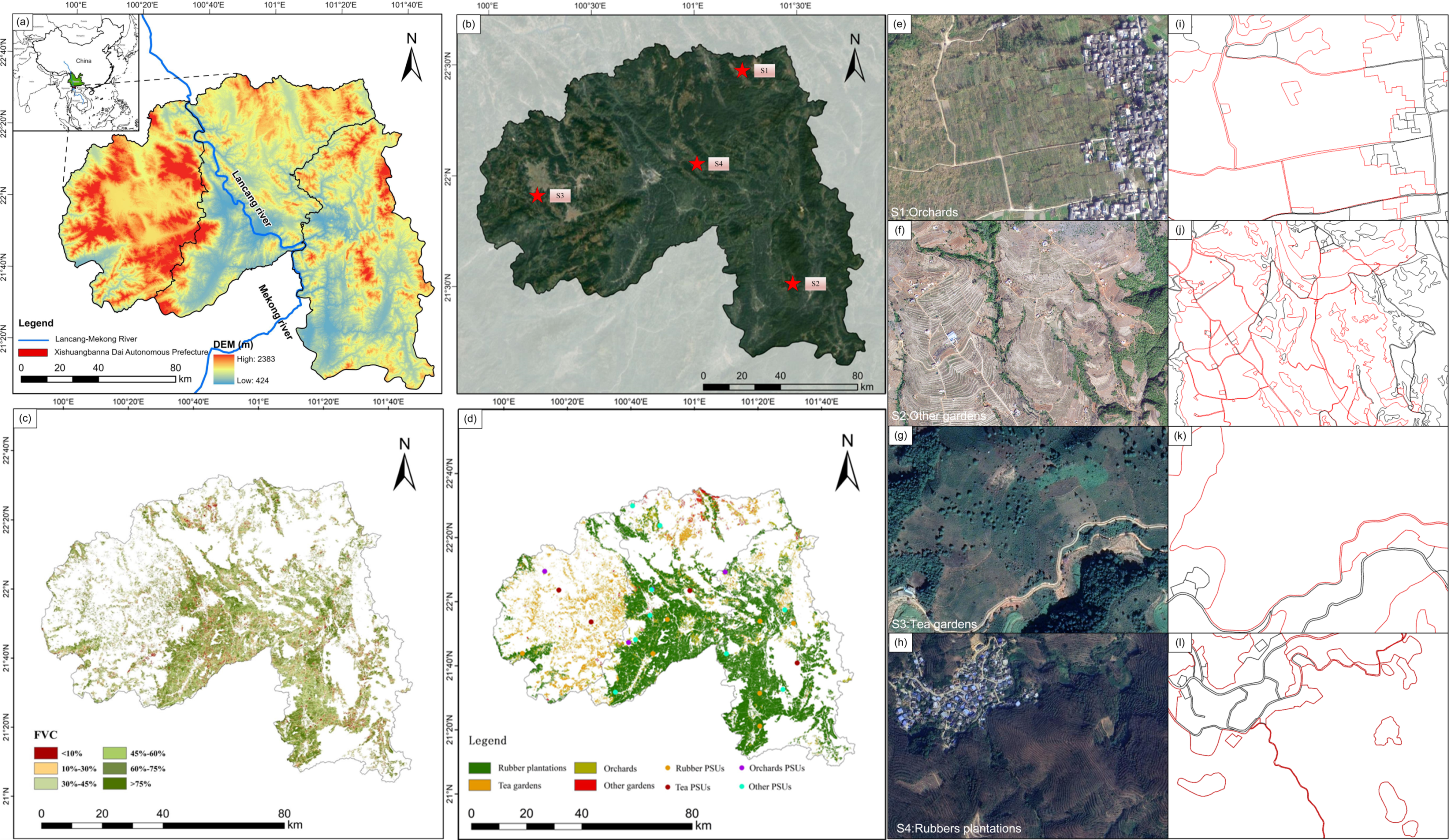
2.1. Study Area
2.2. Data Sources
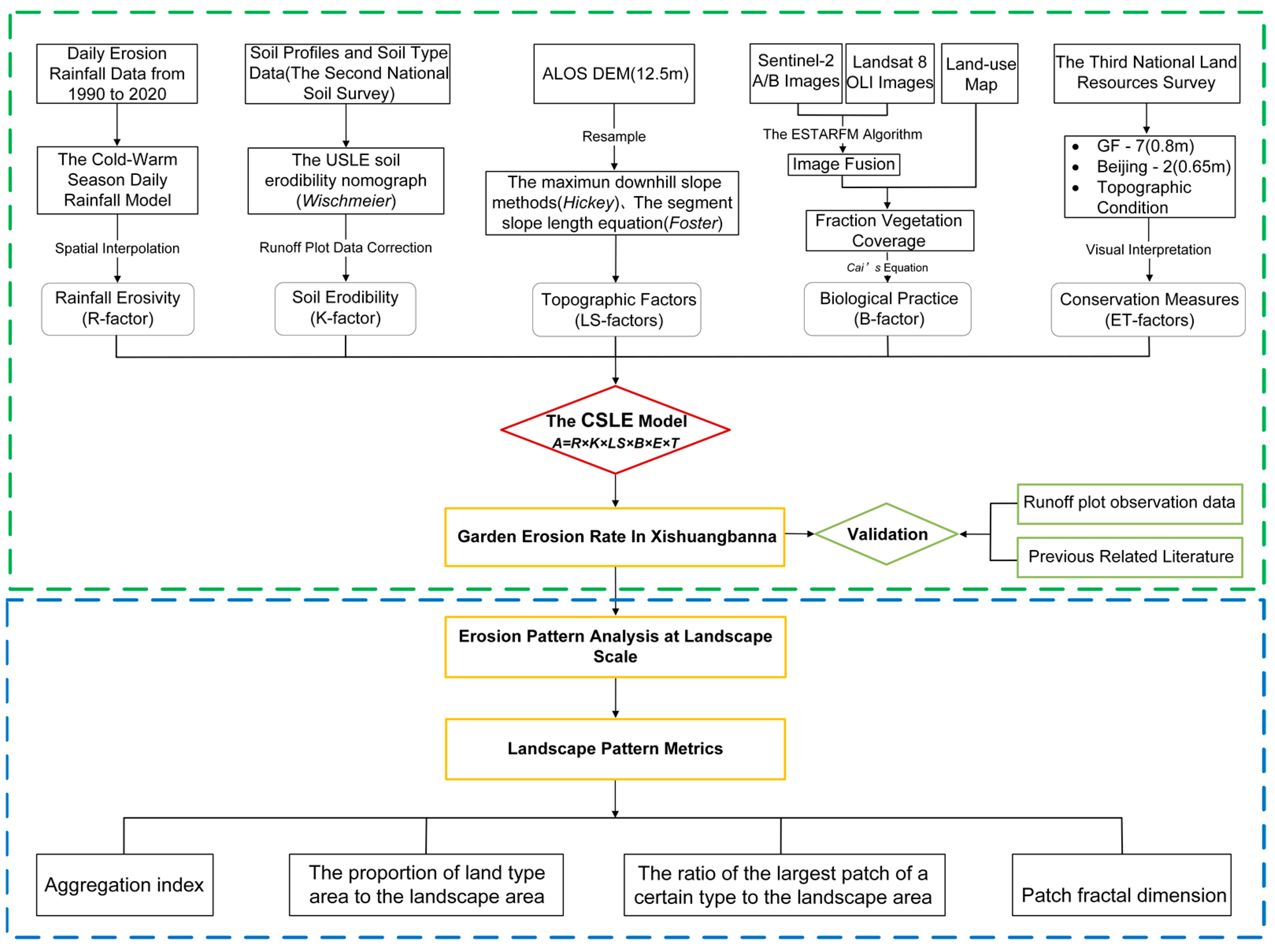
2.3. Methodology
2.3.1. The CSLE Model
2.3.2. Landscape Pattern Metrics
- Patch fractal dimension (D):
- b.
- Ratio of the largest patch of a certain type to the landscape area (LPI):
- c.
- Proportion of land-type area to the landscape area (PLAND):
- d.
- Aggregation index (AI, %):
3. Results
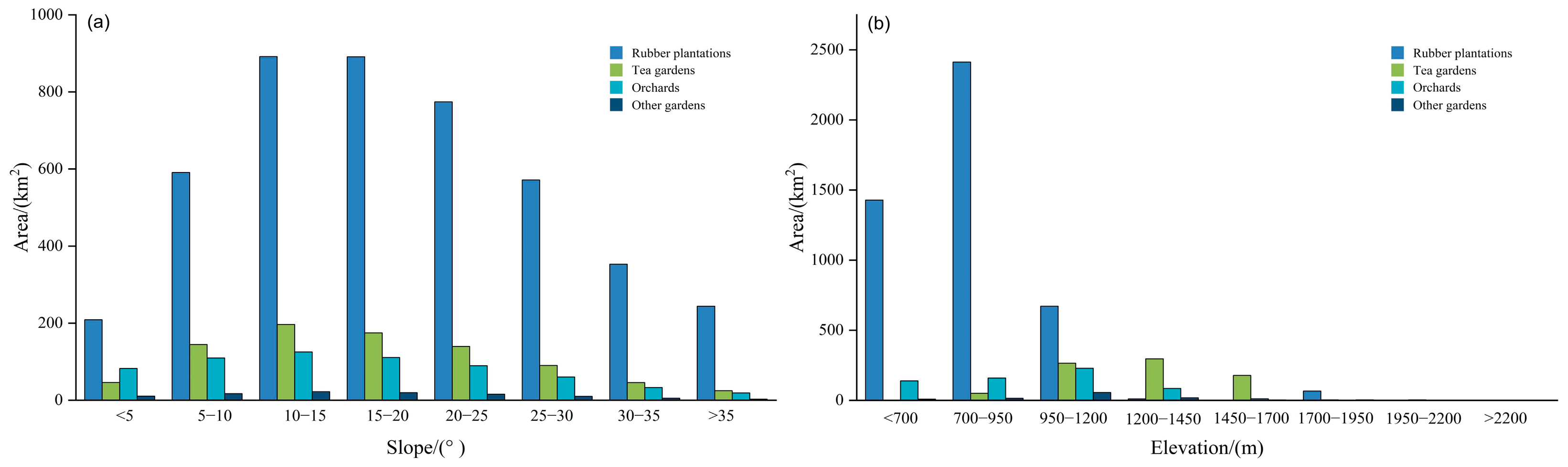
3.1. Spatial Distribution of Garden Plantations in XSBN
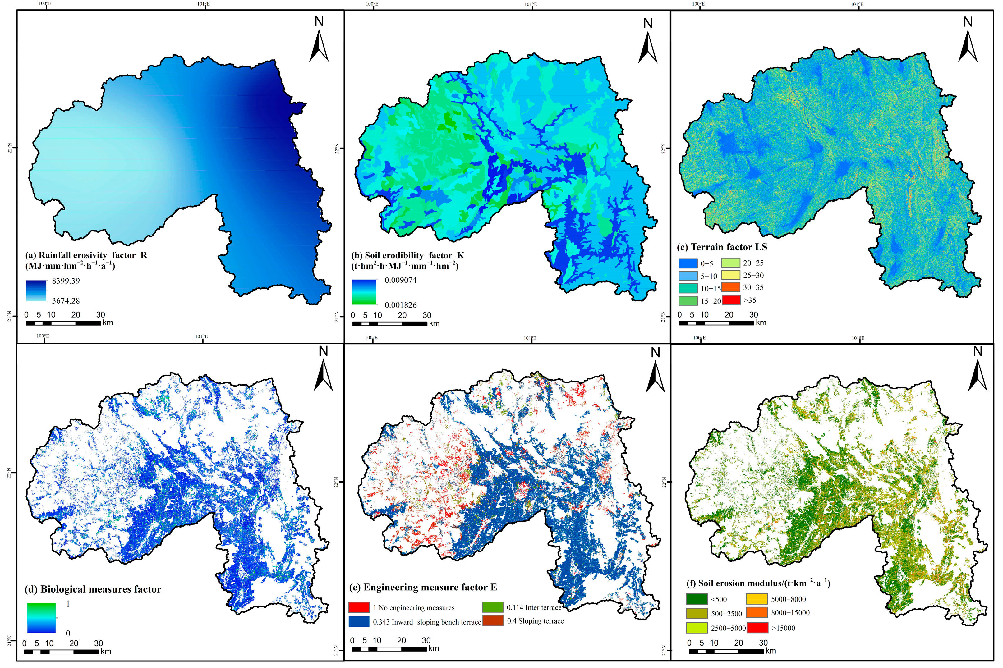
3.2. Spatial Pattern of Garden-Erosion-Affecting Factors
3.3. Soil Erosion of Garden Plantations in XSBN
3.4. Validation of the CSLE Estimated Erosion Rates
3.5. Landscape Pattern of Garden Erosion Intensity
4. Discussion
5. Conclusions
- (1)
- Garden distribution in XSBN shows obvious vertical zoning differentiation, and is more sensitive to altitude change rather than the slope gradient, showing a decreasing trend as the altitude increases. In total, 90% of the gardens in XSBN are distributed in low-altitude areas below 1200 m, of which more than 40% are concentrated in the 700–950-m-altitude zone, much higher than other altitude zones. Orchards and teas are fragmented and mostly planted on slopes, while rubbers are clustered.
- (2)
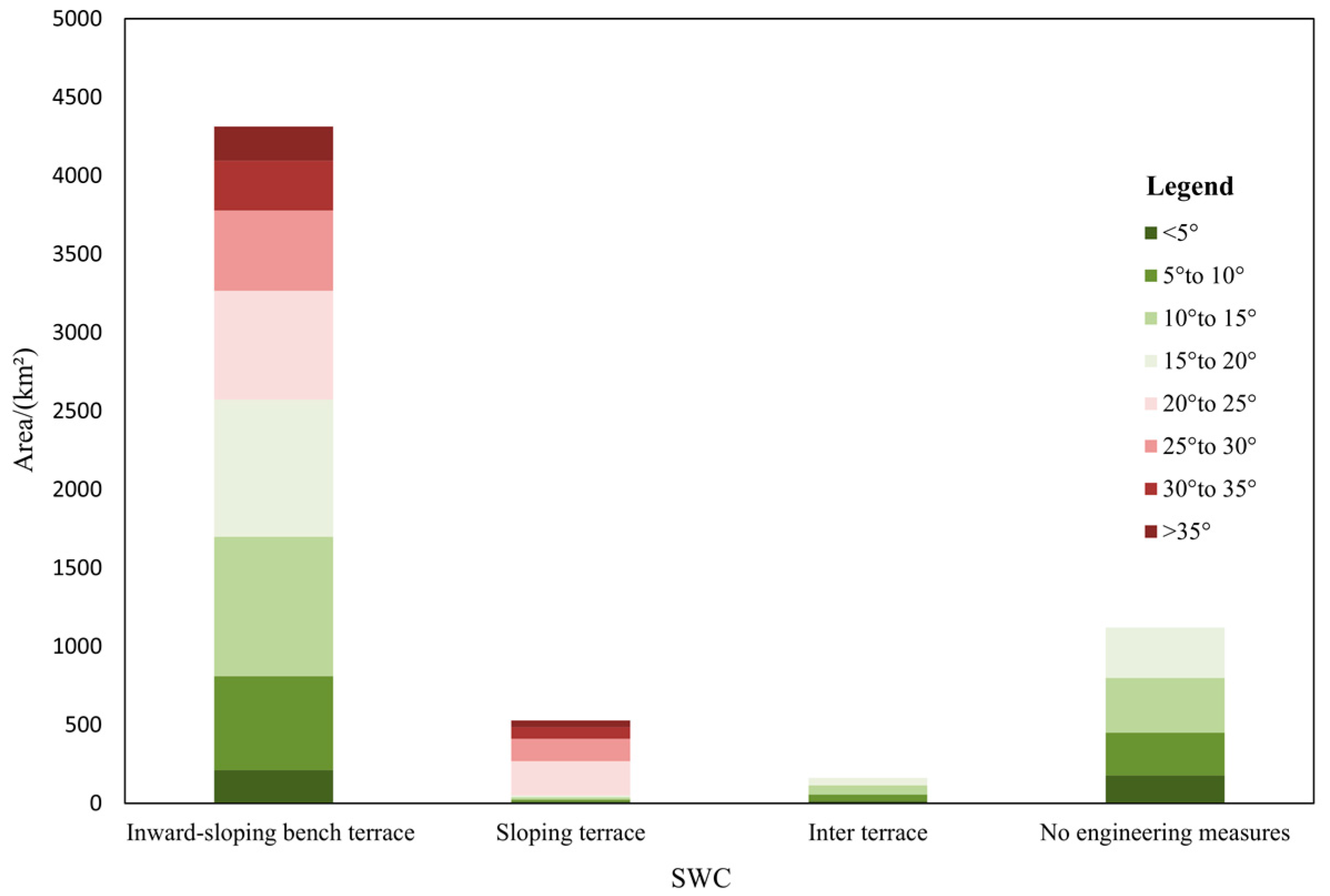
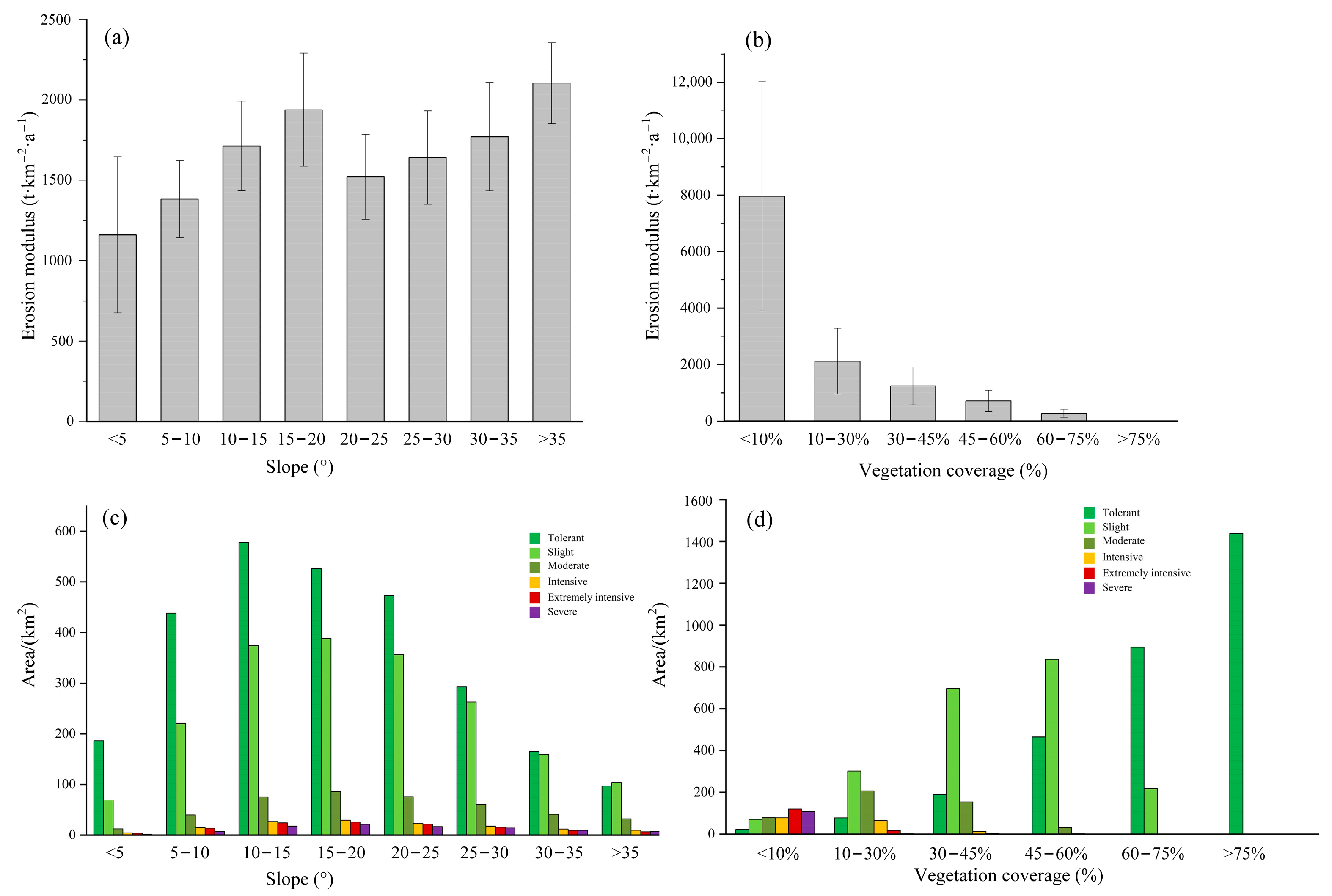
- In total, 49.34% of the gardens in XSBN are being eroded at an erosion rate higher than the soil loss tolerance. The average garden erosion rate in XSBN is 1595.08 t·km−2a−1, which is three times the accepted rate to sustain soil productivity, and the annual soil erosion amount is 9.73 × 10⁶ tons. Extreme and severe erosion are mostly found in those garden lands with FVC lower than 30%, which contribute about 68.19% of the total soil loss. For the three major garden types, orchards suffer from the most serious erosion problem with an erosion rate of 1827.54 t·km−2a−1. Gardens with soil erosion intensity higher than the grade of intensive only account for 6.73% of the total garden area, but contribute more than 50% of the total soil loss amount from gardens. Still, a garden land area of about 1123.93 km² is still under no protection in the prefecture.
- (3)
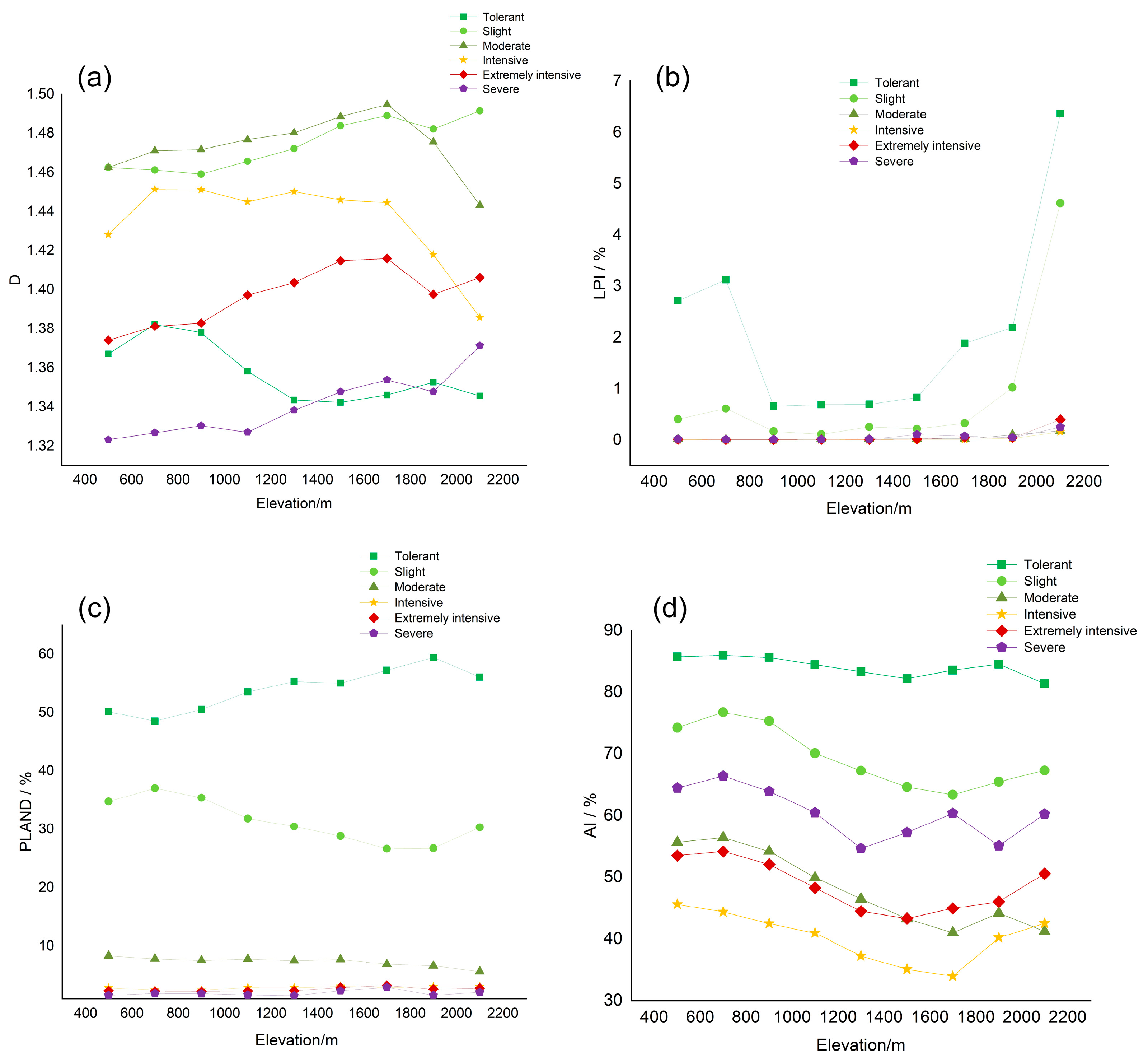
- The spatial analysis of garden erosion intensity demonstrated that heterogeneity in the vertical dimension is much more complex compared to the horizontal dimension. Affected by human activities, garden patches of lowlands (especially near 700 m) are simpler in shape and high in the erosion ratio. Patches of tolerant and slight erosion intensity dominate the landscape, especially in lowlands and areas above 1900 m, showing a high aggregation degree and stability. Meanwhile, garden patches exhibit higher diversity of soil erosion intensity grades in the mid-elevation classes (900–1500 m). The peaks and troughs of landscape metric curves are critical in identifying garden erosion hotspots, for patches that are high in both erosion intensity and aggregation degree can be regarded as priorities of soil erosion control efforts. As the pressure of population and economy growth keeps driving garden plantations onto increasingly steep slopes, soil erosion occurring under a rubber canopy also needs sufficient attention from relevant departments to maintain sustainable development in tropical areas.
Author Contributions
Funding
Data Availability Statement
Acknowledgments
Conflicts of Interest
References
- Morgan, R.P.C. Soil Erosion and Conservation; John Wiley & Sons: New York, NY, USA, 2009. [Google Scholar]
- Borrelli, P.; Robinson, D.A.; Fleischer, L.R.; Lugato, E.; Ballabio, C.; Alewell, C.; Meusburger, K.; Modugno, S.; Schutt, B.; Ferro, V.; et al. An assessment of the global impact of 21st century land use change on soil erosion. Nat. Commun. 2017, 8, 13. [Google Scholar] [CrossRef] [PubMed]
- Liu, B.Y.; Yang, Y.; Lu, S.Y. Discriminations on common soil erosion terms and their implications for soil and water conservation. Sci. Soil Water Conserv. 2018, 16, 10–16. (In Chinese) [Google Scholar]
- Keesstra, S.; Pereira, P.; Novara, A.; Brevik, E.C.; Azorin-Molina, C.; Parras-Alcantara, L.; Jordan, A.; Cerda, A. Effects of soil management techniques on soil water erosion in apricot orchards. Sci. Total Environ. 2016, 551, 357–366. [Google Scholar] [CrossRef] [PubMed]
- Duan, J.; Liu, Y.J.; Yang, J.; Tang, C.J.; Shi, Z.H. Role of groundcover management in controlling soil erosion under extreme rainfall in citrus orchards of southern China. J. Hydrol. 2020, 582, 10. [Google Scholar] [CrossRef]
- Wuepper, D.; Borrelli, P.; Finger, R. Countries and the global rate of soil erosion. Nat. Sustain. 2020, 3, 51–55. [Google Scholar] [CrossRef]
- Borrelli, P.; Ballabio, C.; Yang, J.E.; Robinson, D.A.; Panagos, P. GloSEM: High-resolution global estimates of present and future soil displacement in croplands by water erosion. Sci. Data 2022, 9, 9. [Google Scholar] [CrossRef] [PubMed]
- Kemp, D.B.; Sadler, P.M.; Vanacker, V. The human impact on North American erosion, sediment transfer, and storage in a geologic context. Nat. Commun. 2020, 11, 9. [Google Scholar] [CrossRef]
- Pope, I.; Harbor, J.; Zanotti, L.; Shao, G.; Bowen, D.; Burniske, G.R. Cloud Forest Conservation in the Central Highlands of Guatemala Hinges on Soil Conservation and Intensifying Food Production. Prof. Geogr. 2016, 68, 1–13. [Google Scholar] [CrossRef]
- Meliho, M.; Nouira, A.; Benmansour, M.; Boulmane, M.; Khattabi, A.; Mhammdi, N.; Benkdad, A. Assessment of soil erosion rates in a Mediterranean cultivated and uncultivated soils using fallout 137Cs. J. Environ. Radioact. 2019, 208, 10. [Google Scholar] [CrossRef]
- Guo, L.J.; Liu, R.M.; Men, C.; Wang, Q.R.; Miao, Y.X.; Shoaib, M.; Wang, Y.F.; Jiao, L.J.; Zhang, Y. Multiscale spatiotemporal characteristics of landscape patterns, hotspots, and influencing factors for soil erosion. Sci. Total Environ. 2021, 779, 13. [Google Scholar] [CrossRef]
- Sun, H.L. Chinese Encyclopedia of Resource Science; Encyclopedia of China Publishing House: Beijing, China, 2000; pp. 124–156. [Google Scholar]
- The Detailed Rules for the Land Classification of the Third National Land Survey, Ministry of Natural Resources of the People’s Republic of China. Available online: https://www.mnr.gov.cn/ (accessed on 20 June 2022).
- Liu, X.N.; Feng, Z.M.; Jiang, L.G.; Zhang, J.H. Spatial-Temporal Pattern Analysis of Land Use and Land Cover Change in Xishuangbanna. Resour. Sci. 2014, 36, 233–244. (In Chinese) [Google Scholar]
- Chen, H.F.; Yi, Z.F.; Schmidt-Vogt, D.; Ahrends, A.; Beckschafer, P.; Kleinn, C.; Ranjitkar, S.; Xu, J.C. Pushing the Limits: The Pattern and Dynamics of Rubber Monoculture Expansion in Xishuangbanna, SW China. PLoS ONE 2016, 11, 15. [Google Scholar] [CrossRef]
- Zhu, X.I.; Yuan, X.; Lu, E.F.; Yang, B.; Wang, H.F.; Du, Y.Y.; Singh, A.K.; Liu, W.J. Soil splash erosion: An overlooked issue for sustainable rubber plantation in the tropical region of China. Int. Soil Water Conserv. Res. 2023, 11, 30–42. [Google Scholar] [CrossRef]
- Liu, W.J.; Luo, Q.P.; Lu, H.J.; Wu, J.N.; Duan, W.P. The effect of litter layer on controlling surface runoff and erosion in rubber plantations on tropical mountain slopes, SW China. Catena 2017, 149, 167–175. [Google Scholar] [CrossRef]
- Zhu, X.A.; Chen, C.F.; Wu, J.N.; Yang, J.B.; Zhang, W.J.; Zou, X.; Liu, W.J.; Jiang, X.J. Can intercrops improve soil water infiltrability and preferential flow in rubber-based agroforestry system? Soil Tillage Res. 2019, 191, 327–339. [Google Scholar] [CrossRef]
- Wang, S.S.; Sun, B.Y.; Li, C.D.; Li, Z.B.; Ma, B. Runoff and Soil Erosion on Slope Cropland: A Review. J. Resour. Ecol. 2018, 9, 461–470. [Google Scholar]
- Wang, X.X.; Sun, Y.Y.; Hu, Y.; Zhu, C.J. Impact of Weeds on Surface Runoff and Soil Loss in a Navel Orange Orchard. J. Weed Sci. 2019, 37, 23–28. (In Chinese) [Google Scholar]
- Liu, H.X.; Blagodatsky, S.; Giese, M.; Liu, F.; Xu, J.C.; Cadisch, G. Impact of herbicide application on soil erosion and induced carbon loss in a rubber plantation of Southwest China. Catena 2016, 145, 180–192. [Google Scholar] [CrossRef]
- Sarathchandra, C.; Abebe, Y.A.; Worthy, F.R.; Wijerathne, I.L.; Ma, H.X.; Bi, Y.F.; Guo, J.Y.; Chen, H.F.; Yan, Q.S.; Geng, Y.F.; et al. Impact of land use and land cover changes on carbon storage in rubber dominated tropical Xishuangbanna, South West China. Ecosyst. Health Sustain. 2021, 7, 14. [Google Scholar] [CrossRef]
- Igwe, P.U.; Onuigbo, A.A.; Chinedu, O.C.; Ezeaku, I.I.; Muoneke, M.M. Soil erosion: A review of models and applications. Int. J. Adv. Eng. Res. Sci. 2017, 4, 237341. [Google Scholar]
- Borrelli, P.; Alewell, C.; Alvarez, P.; Anache, J.A.A.; Baartman, J.; Ballabio, C.; Bezak, N.; Biddoccu, M.; Cerda, A.; Chalise, D.; et al. Soil erosion modelling: A global review and statistical analysis. Sci. Total Environ. 2021, 780, 18. [Google Scholar] [CrossRef]
- Laflen, J.M.; Flanagan, D.C. The development of US soil erosion prediction and modeling. Int. Soil Water Conserv. Res. 2013, 1, 1–11. [Google Scholar] [CrossRef]
- Alewell, C.; Borrelli, P.; Meusburger, K.; Panagos, P. Using the USLE: Chances, challenges and limitations of soil erosion modelling. Int. Soil Water Conserv. Res. 2019, 7, 203–225. [Google Scholar] [CrossRef]
- Renard, K.G. Predicting Soil Erosion by Water: A Guide to Conservation Planning with the Revised Universal Soil Loss Equation (RUSLE); ARS: Washington, DC, USA, 2013. [Google Scholar]
- Flanagan, D.C.; Gilley, J.E.; Franti, T.G. Water Erosion Prediction Project (WEPP): Development history, model capabilities, and future enhancements. Trans. ASABE 2007, 50, 1603–1612. [Google Scholar] [CrossRef]
- Taguas, E.V.; Moral, C.; Ayuso, J.L.; Perez, R.; Gomez, J.A. Modeling the spatial distribution of water erosion within a Spanish olive orchard microcatchment using the SEDD model. Geomorphology 2011, 133, 47–56. [Google Scholar] [CrossRef]
- Gharibreza, M.; Samani, A.B.; Arabkhedri, M.V.; Zaman, M.; Porto, P.; Kamali, K.; Sobh-Zahedi, S. Investigation of on-site implications of tea plantations on soil erosion in Iran using Cs-137 method and RUSLE. Environ. Earth Sci. 2021, 80, 14. [Google Scholar] [CrossRef]
- Novara, A.; Gristina, L.; Saladino, S.S.; Santoro, A.; Cerda, A. Soil erosion assessment on tillage and alternative soil managements in a Sicilian vineyard. Soil Tillage Res. 2011, 117, 140–147. [Google Scholar] [CrossRef]
- Niu, Y.H.; Wang, L.; Wan, X.G.; Peng, Q.Z.; Huang, Q.; Shi, Z.H. A systematic review of soil erosion in citrus orchards worldwide. Catena 2021, 206, 9. [Google Scholar] [CrossRef]
- Rodrigo-Comino, J.; Taguas, E.; Seeger, M.; Ries, J.B. Quantification of soil and water losses in an extensive olive orchard catchment in Southern Spain. J. Hydrol. 2018, 556, 749–758. [Google Scholar] [CrossRef]
- Neyret, M.; Robain, H.; de Rouw, A.; Janeau, J.L.; Durand, T.; Kaewthip, J.; Trisophon, K.; Valentin, C. Higher runoff and soil detachment in rubber tree plantations compared to annual cultivation is mitigated by ground cover in steep mountainous Thailand. Catena 2020, 189, 12. [Google Scholar] [CrossRef]
- Ebabu, K.; Tsunekawa, A.; Haregeweyn, N.; Tsubo, M.; Adgo, E.; Fenta, A.A.; Meshesha, D.T.; Berihun, M.L.; Sultan, D.; Vanmaercke, M.; et al. Global analysis of cover management and support practice factors that control soil erosion and conservation. Int. Soil Water Conserv. Res. 2022, 10, 161–176. [Google Scholar] [CrossRef]
- Novara, A.; Cerda, A.; Barone, E.; Gristina, L. Cover crop management and water conservation in vineyard and olive orchards. Soil Tillage Res. 2021, 208, 11. [Google Scholar] [CrossRef]
- Ahmad, N.; Mustafa, F.B.; Yusoff, S.Y.M.; Didams, G. A systematic review of soil erosion control practices on the agricultural land in Asia. Int. Soil Water Conserv. Res. 2020, 8, 103–115. [Google Scholar] [CrossRef]
- Jia, L.Z.; Zhao, W.W.; Zhai, R.J.; Liu, Y.; Kang, M.M.; Zhang, X. Regional differences in the soil and water conservation efficiency of conservation tillage in China. Catena 2019, 175, 18–26. [Google Scholar] [CrossRef]
- Liu, H.X.; Yang, X.Q.; Blagodatsky, S.; Marohn, C.; Liu, F.; Xu, J.C.; Cadisch, G. Modelling weed management strategies to control erosion in rubber plantations. Catena 2019, 172, 345–355. [Google Scholar] [CrossRef]
- Cerda, A.; Rodrigo-Comino, J.; Gimenez-Morera, A.; Novara, A.; Pulido, M.; Kapovic-Solomun, M.; Keesstra, S.D. Policies can help to apply successful strategies to control soil and water losses. The case of chipped pruned branches (CPB) in Mediterranean citrus plantations. Land Use Pol. 2018, 75, 734–745. [Google Scholar] [CrossRef]
- Li, H.Y.; Zhu, N.Y.; Wang, S.C.; Gao, M.N.; Xia, L.Z.; Kerr, P.G.; Wu, Y.H. Dual benefits of long-termecological agricultural engineering: Mitigation of nutrient losses and improvement of soil quality. Sci. Total Environ. 2020, 721, 11. [Google Scholar] [CrossRef]
- Liu, X.Y.; Xin, L.J.; Lu, Y.H. National scale assessment of the soil erosion and conservation function of terraces in China. Ecol. Indic. 2021, 129, 14. [Google Scholar] [CrossRef]
- Sepuru, T.K.; Dube, T. An appraisal on the progress of remote sensing applications in soil erosion mapping and monitoring. Remote Sens. Appl. Soc. Environ. 2018, 9, 1–9. [Google Scholar] [CrossRef]
- King, C.; Baghdadi, N.; Lecomte, V.; Cerdan, O. The application of remote-sensing data to monitoring and modelling of soil erosion. Catena 2005, 62, 79–93. [Google Scholar] [CrossRef]
- Panagos, P.; Ballabio, C.; Poesen, J.; Lugato, E.; Scarpa, S.; Montanarella, L.; Borrelli, P. A soil erosion indicator for supporting agricultural, environmental and climate policies in the European Union. Remote Sens. 2020, 12, 1365. [Google Scholar] [CrossRef]
- Matthews, F.; Verstraeten, G.; Borrelli, P.; Panagos, P. A field parcel-oriented approach to evaluate the crop cover-management factor and time-distributed erosion risk in Europe. Int. Soil Water Conserv. Res. 2023, 11, 43–59. [Google Scholar] [CrossRef]
- Matthews, F.; Panagos, P.; Borrelli, P.; Verstraeten, G. A Crop Phenology-Based Approach to Quantify the C-Factor at the Field-Parcel Scale in Europe; Copernicus Meetings: Vienna, Austria, 2023. [Google Scholar]
- Pijl, A.; Quarella, E.; Vogel, T.A.; D’Agostino, V.; Tarolli, P. Remote sensing vs. field-based monitoring of agricultural terrace degradation. Int. Soil Water Conserv. Res. 2021, 9, 1–10. [Google Scholar] [CrossRef]
- Zhang, F.; Liu, B.Y.; Zhu, L.P.; Cruse, R.; Li, D.F.; Panagos, P.; Borrelli, P.; Kuzyakov, Y.; An, S. Call for joint international actions to improve scientific understanding and address soil erosion and riverine sediment issues in mountainous regions. Int. Soil Water Conserv. Res. 2023, 11, 586–588. [Google Scholar] [CrossRef]
- Matthews, F.; Verstraeten, G.; Borrelli, P.; Vanmaercke, M.; Poesen, J.; Steegen, A.; Degré, A.; Rodríguez, B.C.; Bielders, C.; Franke, C. EUSEDcollab: A network of data from European catchments to monitor net soil erosion by water. Sci. Data 2023, 10, 515. [Google Scholar] [CrossRef]
- Xie, Y.; Yue, Y.T. Application of soil erosion models for soil and water conservation. Sci. Soil Water Conserv. 2018, 16, 25–37. (In Chinese) [Google Scholar]
- Hammond, J.; Yi, Z.; McLellan, T.; Zhao, J. Situational Analysis Report: Xishuangbanna Autonomous Dai Prefecture, Yunnan Province, China; World Agroforestry Centre East and Central Asia: Kunming, China, 2015. [Google Scholar]
- Cao, M.; Zou, X.M.; Warren, M.; Zhu, H. Tropical forests of xishuangbanna, China. Biotropica 2006, 38, 306–309. [Google Scholar] [CrossRef]
- Li, H.M.; Ma, Y.X.; Aide, T.M.; Liu, W.J. Past, present and future land-use in Xishuangbanna, China and the implications for carbon dynamics. For. Ecol. Manag. 2008, 255, 16–24. [Google Scholar] [CrossRef]
- Lü, X.T.; Yin, J.X.; Tang, J.W. Structure, tree species diversity and composition of tropical seasonal rainforests in Xishuangbanna, south-west China. J. Trop. For. Sci. 2010, 22, 260–270. [Google Scholar]
- Zhu, H. Forest vegetation of Xishuangbanna, south China. For. Ecosyst. 2006, 8, 1–58. [Google Scholar]
- Zhang, J.Q.; Corlett, R.T.; Zhai, D.L. After the rubber boom: Good news and bad news for biodiversity in Xishuangbanna, Yunnan, China. Reg. Environ. Chang. 2019, 19, 1713–1724. [Google Scholar] [CrossRef]
- Chen, G.K.; Liu, Z.C.; Wen, Q.K.; Tan, R.; Wang, Y.W.; Zhao, J.J.; Feng, J.X. Identification of Rubber Plantations in Southwestern China Based on Multi-Source Remote Sensing Data and Phenology Windows. Remote Sens. 2023, 15, 1228. [Google Scholar] [CrossRef]
- Chen, G.K.; Zhang, Z.X.; Guo, Q.K.; Wang, X.; Wen, Q.K. Quantitative assessment of soil erosion based on CSLE and the 2010 national soil erosion survey at regional scale in Yunnan Province of China. Sustainability 2019, 11, 3252. [Google Scholar] [CrossRef]
- Chen, G.K.; Wang, Y.W.; Wen, Q.K.; Zuo, L.J.; Zhao, J.J. An Erosion-Based Approach Using Multi-Source Remote Sensing Imagery for Grassland Restoration Patterns in a Plateau Mountainous Region, SW China. Remote Sens. 2023, 15, 2047. [Google Scholar] [CrossRef]
- Liu, B.Y.; Zhang, K.L.; Xie, Y. An empirical soil loss equation. In Proceedings of the 12th International Soil Conservation Organization Conference, Beijing, China, 26–31 May 2002; pp. 21–25. [Google Scholar]
- Liu, B.Y.; Guo, S.; Peichl, M.Z.; Wang, X.J.R.S. Sampling survey of water erosion in China. Soil Water Conserv. China 2017, 10, 26–34. (In Chinese) [Google Scholar]
- Liu, B.Y.; Nearing, M.A.; Shi, P.J.; Jia, Z.W. Slope length effects on soil loss for steep slopes. Soil Sci. Soc. Am. J. 2000, 64, 1759–1763. [Google Scholar] [CrossRef]
- Liu, B.Y.; Xie, Y.; Li, Z.G.; Liang, Y.; Zhang, W.B.; Fu, S.H.; Yin, S.Q.; Wei, X.; Zhang, K.L.; Wang, Z.Q. The assessment of soil loss by water erosion in China. Int. Soil Water Conserv. Res. 2020, 8, 430–439. [Google Scholar] [CrossRef]
- Mccool, D.K.; Brown, L.C.; Foster, G.R.; Mutchler, C.K.; Meyer, L.D. Revised slope steepness factor for the Universal Soil Loss Equation. Trans. ASAE 1987, 30, 1387–1396. [Google Scholar] [CrossRef]
- Liu, B.Y.; Nearing, M.A.; Risse, L.M. Slope gradient effects on soil loss for steep slopes. Trans. ASAE 1994, 37, 1835–1840. [Google Scholar] [CrossRef]
- Yan, K.; Gao, S.; Chi, H.J.; Qi, J.B.; Song, W.J.; Tong, Y.Y.; Mu, X.H.; Yan, G.J. Evaluation of the vegetation-index-based dimidiate pixel model for fractional vegetation cover estimation. IEEE Trans. Geosci. Remote Sens. 2021, 60, 1–14. [Google Scholar]
- Cai, C.F.; Ding, S.W.; Shi, Z.H.; Huang, L.; Zhang, G.Y. Study of applying USLE and geographical information system IDRISI to predict soil erosion in small watershed. J. Soil Water Conserv. 2000, 14, 19–24. [Google Scholar]
- Duan, X.; Rong, L.; Bai, Z.; Gu, Z.; Ding, J.; Tao, Y.; Li, J.; Wang, W.; Yin, X. Effects of soil conservation measures on soil erosion in the Yunnan Plateau, southwest China. J. Soil Water Conserv. 2020, 75, 131–142. [Google Scholar] [CrossRef]
- Duan, X.W.; Bai, Z.W.; Rong, L.; Li, Y.B.; Ding, J.H.; Tao, Y.Q.; Li, J.X.; Li, J.S.; Wang, W. Investigation method for regional soil erosion based on the Chinese Soil Loss Equation and high-resolution spatial data: Case study on the mountainous Yunnan Province, China. Catena 2020, 184, 104237. [Google Scholar] [CrossRef]
- Chen, L.D.; Liu, Y.; Lu, Y.H. Landscape pattern analysis in landscape ecology: Current, challenges andfuture. Acta Ecol. Sin. 2008, 28, 5521–5531. [Google Scholar]
- Liu, Y.; Lu, Y.; Fu, B.J. Implication and limitation of landscape metrics in delineating relationship between landscape pattern and soil erosion. Acta Ecol. Sin. 2011, 31, 267–275. (In Chinese) [Google Scholar]
- Wang, Y.W.; Liu, Q.J.; Yu, X.X. Fractal characteristics of vertical landscape of soil erosion in the Yimeng mountainous area. Trans. Chin. Soc. Agric. Eng. 2010, 26, 304–309. (In Chinese) [Google Scholar]
- Liu, Q.J.; Yu, X.X. Vertical landscape pattern on soil erosion intensity in the rocky area of northern China: A case study in the Yimeng Mountainous Area Shandong. Geogr. Res. 2010, 29, 1471–1483. [Google Scholar]
- Song, S.; Wang, S.H.; Shi, M.X.; Hu, S.S.; Xu, D.W. Influences of landscape pattern on water quality at multiple scales in an agricultural basin of western China. Res. Soil Water Conserv. 2023, 29, 120986. (In Chinese) [Google Scholar]
- Liu, Y. Effectiveness of landscape metrics in coupling soil erosion with landscape pattern. Acta Ecol. Sin. 2017, 37, 4923–4935. (In Chinese) [Google Scholar]


| Measures | Descriptions and Interpretation Symbols | Remote Sensing Images | E Value |
|---|---|---|---|
| Interval terrace (IT) | Double terraces, with a flat surface interspersed within slopes. Each level terrace has an area of the original slope above; an evident natural slope between two terraces in the remote sensing images |  | 0.114 |
| Sloping terrace (ST) | Horizontal terraces with lower ridges compared to ISBT, uneven surface, curved shape in remote sensing images and less regular and wider than ISBT; mostly distributed in areas with slopes greater than 5° and planted with different crops |  | 0.393 |
| Inward (reverse) sloping bench terrace (ISBT) | Slopes transformed into terraces of 1–1.5 m width, with terrace surfaces sloping inwards at 3–5°; regular strip shape in remote sensing images, mostly on slopes, planted with teas and citrus |  | 0.343 |
| Gardens | NP | LA (km2) | MPA (km2) | MPS (m2) | MPM (km2) | SD (km2) |
|---|---|---|---|---|---|---|
| Tea gardens | 31326 | 863.639 | 2.564 | 61.187 | 0.028 | 0.076 |
| Orchards | 21092 | 630.566 | 1.974 | 71.195 | 0.030 | 0.069 |
| Rubbers | 26098 | 4528.892 | 22.375 | 60.885 | 0.174 | 0.742 |
| Other gardens | 5074 | 102.966 | 1.019 | 56.982 | 0.020 | 0.047 |
| Erosion Intensity | SER/(t·km−2a−1) | Area/km2 | AP/% | SL/106 t | SLP/% |
|---|---|---|---|---|---|
| Tolerant | <500 | 3089.34 | 50.65 | 0.391 | 4.02 |
| Slight | 500–2500 | 2125.09 | 34.84 | 2.565 | 26.37 |
| Moderate | 2500–5000 | 473.99 | 7.77 | 1.631 | 16.77 |
| Intensive | 5000–8000 | 159.47 | 2.61 | 0.998 | 10.26 |
| Extremely Intensive | 8000–15,000 | 141.28 | 2.32 | 1.546 | 15.90 |
| Severe | >15,000 | 109.63 | 1.80 | 2.596 | 26.69 |
| Gardens | Land Area (km2) | ER | SL/106 t | SLP | |||||
|---|---|---|---|---|---|---|---|---|---|
| T | Sl | M | I | EI | SE | ||||
| Rubbers | 2244.74 | 1631.13 | 342.70 | 108.45 | 101.51 | 80.72 | 50.22% | 7.06 | 72.03% |
| Tea gardens | 465.48 | 268.25 | 66.45 | 25.73 | 20.82 | 14.49 | 45.95% | 1.37 | 14.08% |
| Orchards | 317.08 | 199.09 | 58.50 | 22.82 | 16.76 | 12.24 | 49.39% | 1.14 | 11.77% |
| Other gardens | 62.05 | 26.62 | 6.33 | 2.47 | 2.19 | 2.18 | 39.07% | 0.16 | 1.62% |
| PSUs | Area (ha) | Slope length (m) | Gradient (°) | Longitude | Latitude | NSES (t·ha−1a−1) | Estimation (t·ha−1a−1) | Plantations |
|---|---|---|---|---|---|---|---|---|
| 1 | 1.68 | 52.16 | 24.35 | 100°27′31″ | 21°53′38″ | 7.356 | 11.687 | Tea |
| 2 | 2.23 | 53.40 | 18.69 | 100°17′20″ | 22°03′33″ | 2.255 | 3.903 | Tea |
| 3 | 19.15 | 66.25 | 23.24 | 100°05′56″ | 21°43′53″ | 17.724 | 14.394 | Rubber |
| 4 | 0.74 | 99.35 | 24.37 | 100°35′08″ | 21°31′39″ | 0.534 | 1.605 | Other garden |
| 5 | 0.85 | 32.33 | 18.48 | 100°35′13″ | 22°26′09″ | 2.865 | 1.779 | Other garden |
| 6 | 0.68 | 27.41 | 5.72 | 100°47′25″ | 22°26′27″ | 99.949 | 79.615 | Other garden |
| 7 | 0.47 | 73.76 | 28.53 | 100°46′35″ | 22°03′50″ | 8.647 | 5.540 | Orchard |
| 8 | 2.05 | 96.16 | 33.59 | 100°46′33″ | 22°03′35″ | 13.761 | 8.150 | Other garden |
| 9 | 0.61 | 36.92 | 21.39 | 100°46′37″ | 22°03′43″ | 6.364 | 4.133 | Orchard |
| 10 | 0.26 | 42.94 | 33.88 | 100°46′31″ | 22°03′31″ | 5.800 | 7.297 | Orchard |
| 11 | 0.55 | 46.31 | 30.04 | 100°46′34″ | 21°03′32″ | 19.938 | 21.158 | Orchard |
| 12 | 0.32 | 39.00 | 27.83 | 100°46′34″ | 21°53′56″ | 2.534 | 3.950 | Other garden |
| 13 | 19.73 | 48.39 | 22.80 | 100°46′44″ | 21°53′55″ | 14.809 | 11.101 | Rubber |
| 14 | 1.24 | 60.85 | 28.33 | 100°46′55″ | 21°44′01″ | 40.012 | 26.391 | Rubber |
| 15 | 3.31 | 51.53 | 18.63 | 100°46′50″ | 21°44′05″ | 11.777 | 17.229 | Other garden |
| 16 | 4.27 | 70.06 | 23.92 | 100°58′39″ | 22°03′25″ | 2.774 | 2.836 | Tea |
| 17 | 35.34 | 50.26 | 24.32 | 101°20′41″ | 21°53′51″ | 6.575 | 3.470 | Rubber |
| 18 | 3.19 | 39.14 | 17.08 | 101°31′32″ | 21°53′27″ | 27.515 | 42.409 | Rubber |
| 19 | 0.58 | 62.02 | 29.65 | 101°31′34″ | 21°53′20″ | 13.472 | 21.506 | Other garden |
| 20 | 9.65 | 62.52 | 31.38 | 101°10′05″ | 21°43′40″ | 1.142 | 0.722 | Other garden |
| 21 | 2.86 | 75.86 | 14.77 | 101°32′23″ | 21°43′39″ | 89.668 | 97.613 | Other garden |
| 22 | 2.45 | 40.10 | 18.64 | 101°32′23″ | 21°43′35″ | 17.969 | 12.003 | Tea |
| 23 | 24.14 | 48.38 | 17.56 | 101°20′33″ | 21°31′18″ | 5.481 | 5.333 | Rubber |
| 24 | 0.25 | 55.54 | 36.88 | 101°20′31″ | 21°21′01″ | 9.507 | 7.942 | Rubber |
Disclaimer/Publisher’s Note: The statements, opinions and data contained in all publications are solely those of the individual author(s) and contributor(s) and not of MDPI and/or the editor(s). MDPI and/or the editor(s) disclaim responsibility for any injury to people or property resulting from any ideas, methods, instructions or products referred to in the content. |
© 2023 by the authors. Licensee MDPI, Basel, Switzerland. This article is an open access article distributed under the terms and conditions of the Creative Commons Attribution (CC BY) license (https://creativecommons.org/licenses/by/4.0/).
Share and Cite
Tan, R.; Chen, G.; Tang, B.; Huang, Y.; Ma, X.; Liu, Z.; Feng, J. Landscape Pattern of Sloping Garden Erosion Based on CSLE and Multi-Source Satellite Imagery in Tropical Xishuangbanna, Southwest China. Remote Sens. 2023, 15, 5613. https://doi.org/10.3390/rs15235613
Tan R, Chen G, Tang B, Huang Y, Ma X, Liu Z, Feng J. Landscape Pattern of Sloping Garden Erosion Based on CSLE and Multi-Source Satellite Imagery in Tropical Xishuangbanna, Southwest China. Remote Sensing. 2023; 15(23):5613. https://doi.org/10.3390/rs15235613
Chicago/Turabian StyleTan, Rui, Guokun Chen, Bohui Tang, Yizhong Huang, Xianguang Ma, Zicheng Liu, and Junxin Feng. 2023. "Landscape Pattern of Sloping Garden Erosion Based on CSLE and Multi-Source Satellite Imagery in Tropical Xishuangbanna, Southwest China" Remote Sensing 15, no. 23: 5613. https://doi.org/10.3390/rs15235613