
Distribution Characteristics and Influencing Factors of Sea Ice Leads in the Weddell Sea, Antarctica
by
 , , ,
, , ,
Yueyun Wang
1,
Qing Ji
2,
Xiaoping Pang
1,3,*,
Meng Qu
4,
Mingxing Cha
1,
Fanyi Zhang
1,
Zhongnan Yan
1 and
Bin He
1 1
Chinese Antarctic Center of Surveying and Mapping, Wuhan University, Wuhan 430079, China
2
School of Geography and Tourism, Anhui Normal University, Wuhu 241002, China
3
Key Laboratory of Polar Environment Monitoring and Public Governance, Wuhan University, Ministry of Education, Wuhan 430079, China
4
Key Laboratory of Polar Science of Ministry of Natural Resources, Polar Research Institute of China, Shanghai 200136, China
*
Author to whom correspondence should be addressed.
Remote Sens. 2023, 15(23), 5568; https://doi.org/10.3390/rs15235568
Submission received: 12 October 2023
/
Revised: 17 November 2023
/
Accepted: 28 November 2023
/
Published: 30 November 2023
(This article belongs to the Special Issue Remote Sensing of Polar Sea Ice)
Abstract
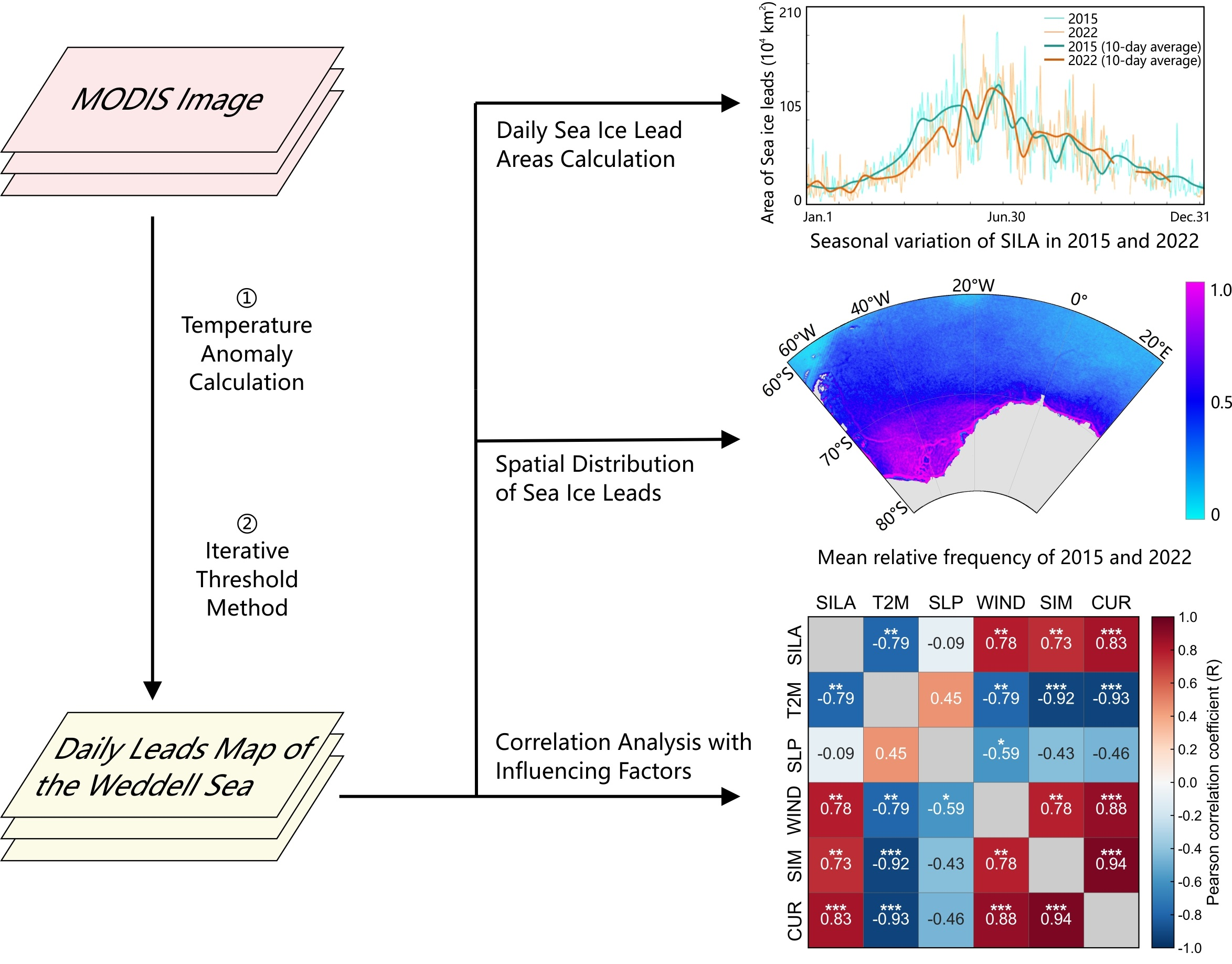
:The characteristics of sea ice leads (SILs) in the Weddell Sea are an important basis for understanding the mechanism of the atmosphere–ocean system in the Southern Ocean. In this study, we derived the sea ice surface temperature (IST) of the Weddell Sea from MODIS thermal images and then generated a daily SIL map for 2015 and 2022 by utilizing the iterative threshold method on the optimised MOD35 cloud-masked IST. The results showed that SIL variations in the Weddell Sea presented remarkable seasonal characteristics. The trend of the SIL area exhibited an initial rise followed by a decline from January to December, characterised by lower values in spring and summer and higher values in fall and winter. SILs in the Weddell Sea were predominantly concentrated between 70~78°S and 60~30°W. The coastal spatial distribution density of the SILs exceeded that of offshore regions, peaking near the Antarctic Peninsula and then near Queen Maud Land. The SIL variation was mainly influenced by dynamical factors, and there were strong positive correlations between the wind field, ocean currents, and sea-ice motion.

1. Introduction
The Antarctic climate system is a critical constituent of the global climatic framework [1,2], and the growth and melting of sea ice in the Antarctic profoundly influence the exchange of heat, momentum, and material between the atmosphere and the ocean [3]. Over the past several decades, the Antarctic sea ice extent (SIE) has exhibited a prolonged period of relatively stable and gradual expansion [3,4]. However, this trend has undergone an abrupt shift towards reduction [5,6], notably in recent years, marked by recurrent instances of record minima [7,8]. The Weddell Sea is one of the prominently diminishing regions of sea ice in the Southern Ocean, and sea ice variations in the Weddell Sea significantly implicate the Southern Ocean [9].
Sea ice leads (SILs), as an important feature of sea ice dynamics, are elongated open water areas formed by the fracturing of sea ice due to joint atmospheric and oceanic forces during motion [10]. Turbulent heat fluxes through SILs during the freezing period of sea ice are two orders of magnitude greater than those through thicker ice [11], which causes them to be a crucial part of the energy exchange between the atmosphere and the ocean [12,13]. In the Weddell Sea, SILs contribute approximately 30% to the total energy flux from the ocean to the atmosphere in winter months [14]. Evidently, SILs serve as a window for exploring polar climate variations. At present, most pertinent research has been conducted in the Arctic region. The initial research mostly focused on the spatial distribution and morphological features, such as width, direction, and length [15,16,17]. Later, it expanded to the turbulent heat flux in SILs [18,19]. Subsequently, researchers used SIL as a predictive factor to forecast the SIE of Arctic summer [20].
In contrast, research on Antarctica SIL primarily focused on the identification algorithm [21,22], and there is a need for more comprehensive research to explore the distribution characteristics of SILs and their correlation with meteorological and hydrological factors. A notable oceanographic feature in the Southern Ocean is the Weddell Gyre (WG). Influenced by the WG, the sea ice in the Weddell Sea moves at higher speeds and is more prone to cracking, forming leads [23]. Furthermore, the Weddell Sea contributes nearly half of the global Antarctic Bottom Water through the Weddell Sea Deep Water and denser Weddell Sea Bottom Water (WSBW) formed on the continental shelves through sea ice production, and the reduction in WSBW is strongly correlated with the decrease rate of sea ice formation [24]. Since SILs are the main sites for sea ice formation [25], studying the distribution characteristics and factors influencing SILs in the Weddell Sea could be a foundation for analysing Antarctic sea ice variations and explaining the mechanisms of the climate system of the Southern Ocean.
In this study, we used MODIS thermal images to retrieve the daily leads distribution of the Weddell Sea using the iterative threshold method. Based on the daily leads map, we analysed the spatiotemporal changes in SIL in the Weddell Sea and explored the correlation between SILs and related thermodynamic and kinetic factors. The data and method used in this study are described in Section 2. The results of the analysis are presented in Section 3, followed by the discussion presented in Section 4. Finally, we conclude our work in Section 5.
2. Data and Methods
2.1. Data Used in This Study
The study area selected for this research was the Weddell Sea sector from 60°W to 20°E and 60°S to 80°S. The utilised data included MODIS data for SIL identification and Sentinel-2 data for accuracy evaluation. Additionally, sea ice concentration products from the University of Bremen, 2 m air temperature, sea level pressure, 10 m wind field products from the European Centre for Medium-Range Weather Forecasts (ECMWF) reanalysis data, sea ice motion vector products from the National Snow and Ice Data Center (NSIDC), and ocean current products from the National Centers for Environmental Prediction (NCEP) reanalysis data were used for correlation analysis.
2.1.1. MODIS Data
The moderate-resolution imaging spectroradiometer (MODIS) is a large-space remote sensing instrument developed by the National Aeronautics and Space Administration (NASA), which is an important payload of the Terra and Aqua satellites mounted on the Earth Observing System (EOS). MODIS has 36 imaging bands, covering the optical and infrared spectral bands from 0.4 μm to 14.4 μm, with ground resolutions of 250 m (bands 1–2), 500 m (bands 3–7) and 1 km (bands 8–36). The MODIS data used in this paper were MODIS L1B-level images (i.e., MOD02 products) and L2-level cloud masks (i.e., MOD35 products) for 2015 and 2022 from NASA’s L1-level Distributed Data Center website (http://ladsweb.nascom.nasa.gov/ (accessed on 27 November 2023)).
2.1.2. Sentinel-2 Data
Sentinel-2 is the European Space Agency (ESA) Copernicus Sentinel missions in the high-resolution multispectral imaging satellites, and its payload is the multispectral imaging instrument (MSI). Sentinel-2 is mainly used for land monitoring, providing images of vegetation, soil and water cover, inland waterways, coastal areas, etc. The Sentinel-2 data released by the ESA are mainly L1C-level geolocated imagery products (https://scihub.copern-icus.eu/dhus/#/home (accessed on 27 November 2023)), with the images projected on the UTM/WGS84 coordinate system and uniformly cropped to 100 km-wide tiles. There are sparse observational images in the polar marine region, and in this paper, four views of Sentinel-2B fourth-band 10 m resolution images in the Weddell Sea were used for leads’ identification accuracy evaluation.
2.1.3. Sea Ice Concentration and Sea Ice Motion Product
The sea ice concentration product was published by the University of Bremen and was based on the AMSR2 (89 GHz) mounted on GCOM-W1, inverted using the ARTIST Sea Ice (ASI) algorithm [26]. The sea ice motion vector data were the daily averaged polar region sea ice motion vector dataset published by NSIDC, which were obtained by applying feature recognition tracking and mutual correlation methods to continuously observed passive microwave imagery extracted and interpolated in combination with International Arctic Buoy Programme (IABP) buoys and NCEP reanalysis wind field data.
2.1.4. Reanalysis Data
ERA5 is the latest generation of ECMWF reanalysis datasets, which is based on a four-dimensional variational data assimilation model and an integrated forecasting system (IFS) to produce predictions of various climate variables in the atmosphere, land and oceans. ERA5 is vertically capable of providing data with a total of 37 atmospheric pressure levels of profiles ranging from 1000 hPa to 1 hPa and horizontally in a latitude–longitude grid. Atmospheric data are provided vertically in a latitude/longitude grid and horizontally at a spatial resolution of 0.25°.
The Climate Forecast System Reanalysis (CFSR) is high-resolution reanalysis data provided by NCEP, covering the globe from 1979 to the present. The atmospheric model used in the CFSR is T382L64 (with a horizontal resolution of ~38 km), with a vertical resolution extending from the surface to 0.26 hPa in 64 layers.
2.2. The Sea Ice Leads Identification Algorithm
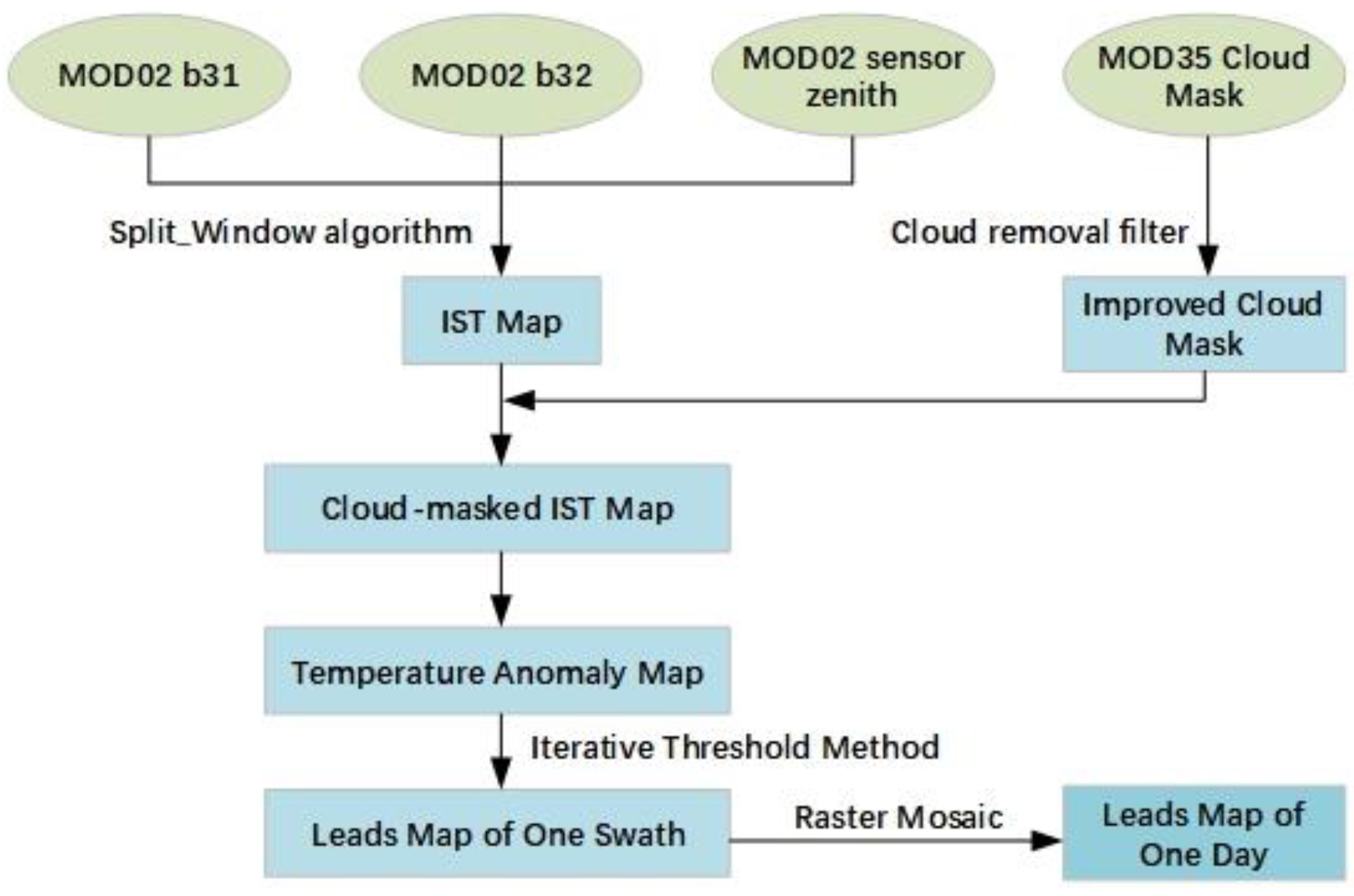
Basically, the retrieval of SILs based on MODIS data is achieved through the differentiation of the surface temperature between sea ice and open water. Utilising the MOD/MYD29 ice surface temperature (IST) product, Willmes and Heinemann (2015) [16] compared several threshold methods for the identification and found that the iterative threshold method is most consistent with the visual interpretation results. Hoffman et al. (2019) [27] opted to utilise the brightness temperature from MOD02/MYD02 instead of the MOD/MYD29 IST product for leads identification due to issues with inappropriate cloud masks in the latter. However, the brightness temperature is susceptible to atmospheric constituents such as water vapour and aerosols, which might hinder an accurate representation of the true temperature difference at the surface [28]. To improve the accuracy of the identification results, we first calculated the IST of the Weddell Sea based on the 31 and 32 bands in MOD02 with the split-window algorithm [28,29]. Second, we optimised the MOD35 product using the method mentioned in Fraser et al. (2009) [30] and applied it to the IST images to eliminate cloudy pixels. Afterwards, the surface temperature anomalies were computed, and the leads map of one swath of MODIS images was generated using the iterative threshold method. Finally, we obtained the daily leads map of the Weddell Sea through raster mosaic. The above process is depicted in Figure 1.
2.3. Precision Evaluation
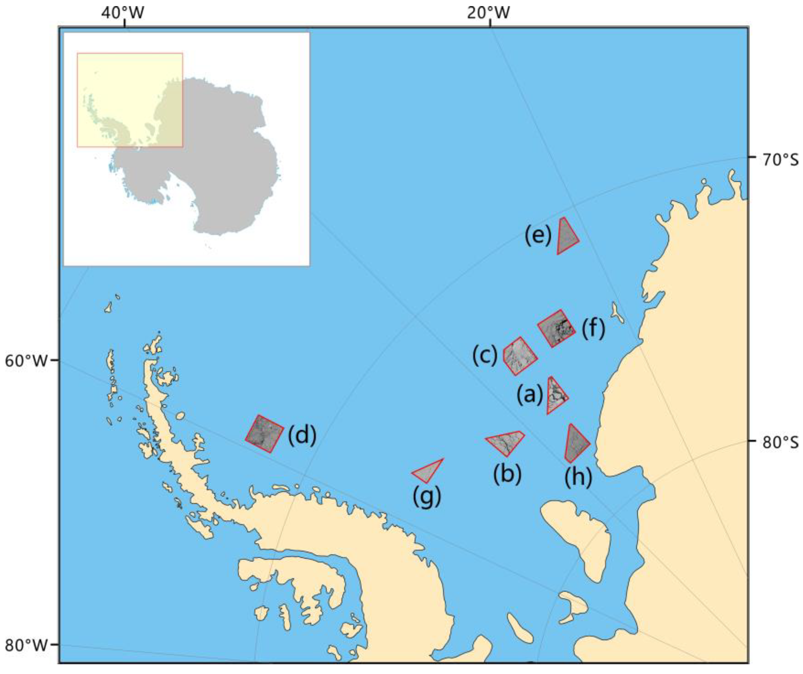
Due to the absence of SIL data observed in situ in Antarctic, we thought Sentinel-2 would be a suitable choice for validating our identification with its resolution capability of up to 10 m. However, Sentinel-2 is not only a land mission that acquires data over oceans only in the vicinity of land [31], which restricts the regional selection, but the polar night phenomenon also has an impact on the image of the Weddell Sea, which further restricts the time selection. In addition, cloud cover also affects the validation results. Therefore, in this study, we manually selected eight cloud-free images with the period ranges from September to March for the evaluation of the experimental results. The distribution of the used data is shown in Figure 2.
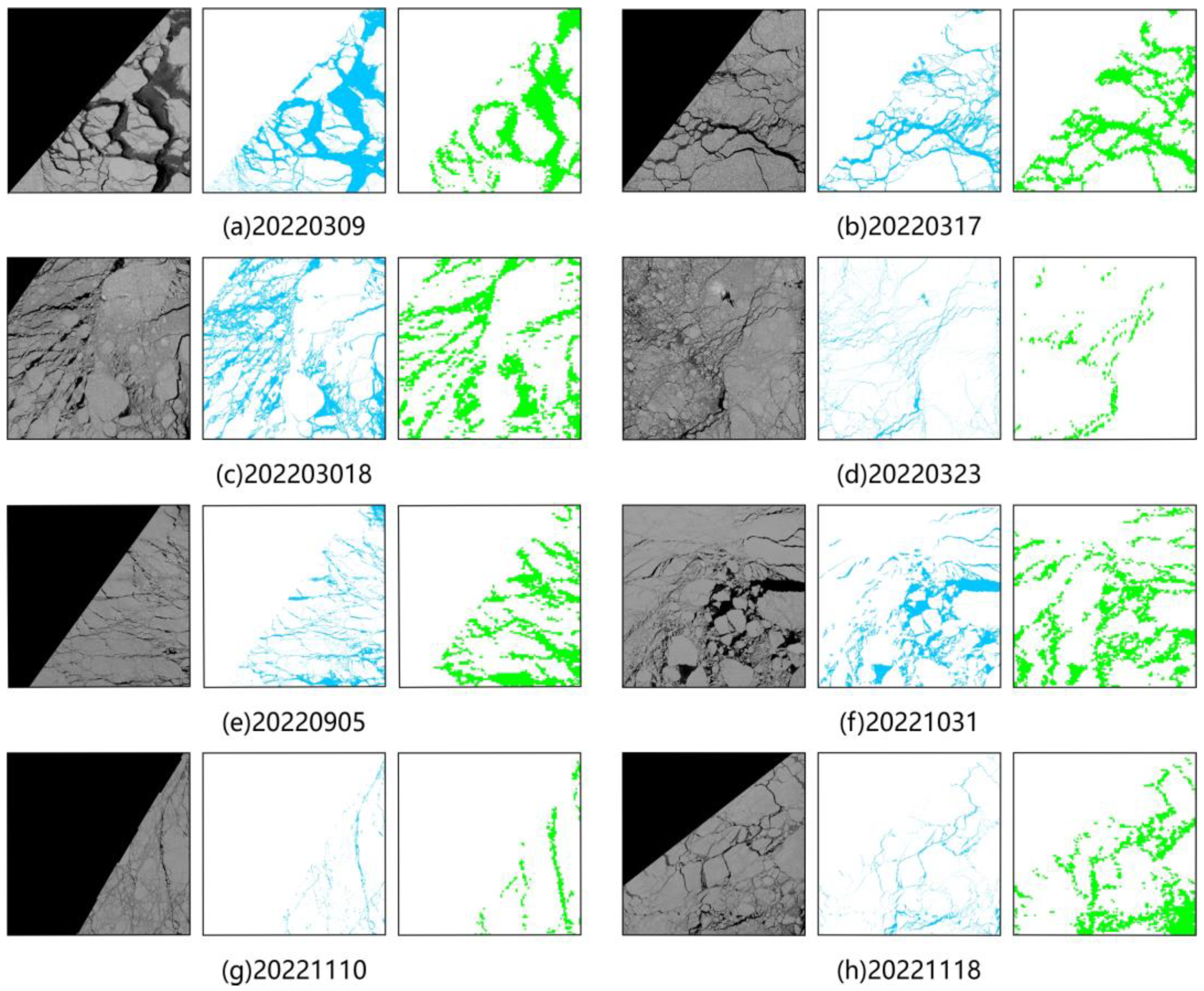
A previous study showed that band 4 (665 nm) of Sentinel-2 is the best choice for SIL identification [22]; thus, the reflectance of band 4 was chosen for comparison with the identification results for evaluation in this paper. The comparison of SILs detected from Sentinel-2 images and MODIS images is depicted in Figure 3, which is arranged in the order, Sentinel-2 original band 4 image, Sentinel-2 leads map, and MODIS leads map. And the sensing date, the product name and the precision result of each image are shown in Table 1.
The results above show that the SILs with a width exceeding 1 km were clearly identified based on MODIS images. Overall, our algorithm exhibited the capability to accurately identify 87.16% of the lead structures.
3. Results
3.1. Temporal Variation in Sea Ice Leads Area
On 19 September 2014, Antarctic sea ice reached a record maximum extent of 20 million square kilometres, marking the largest extent in a dataset that commenced in 1978 [32]. Subsequently, the total Antarctic SIE began to decline [33]. Therefore, 2015 represents a pivotal inflection point in the dynamics of Antarctic sea ice variation, and is designated as the starting point for this study.
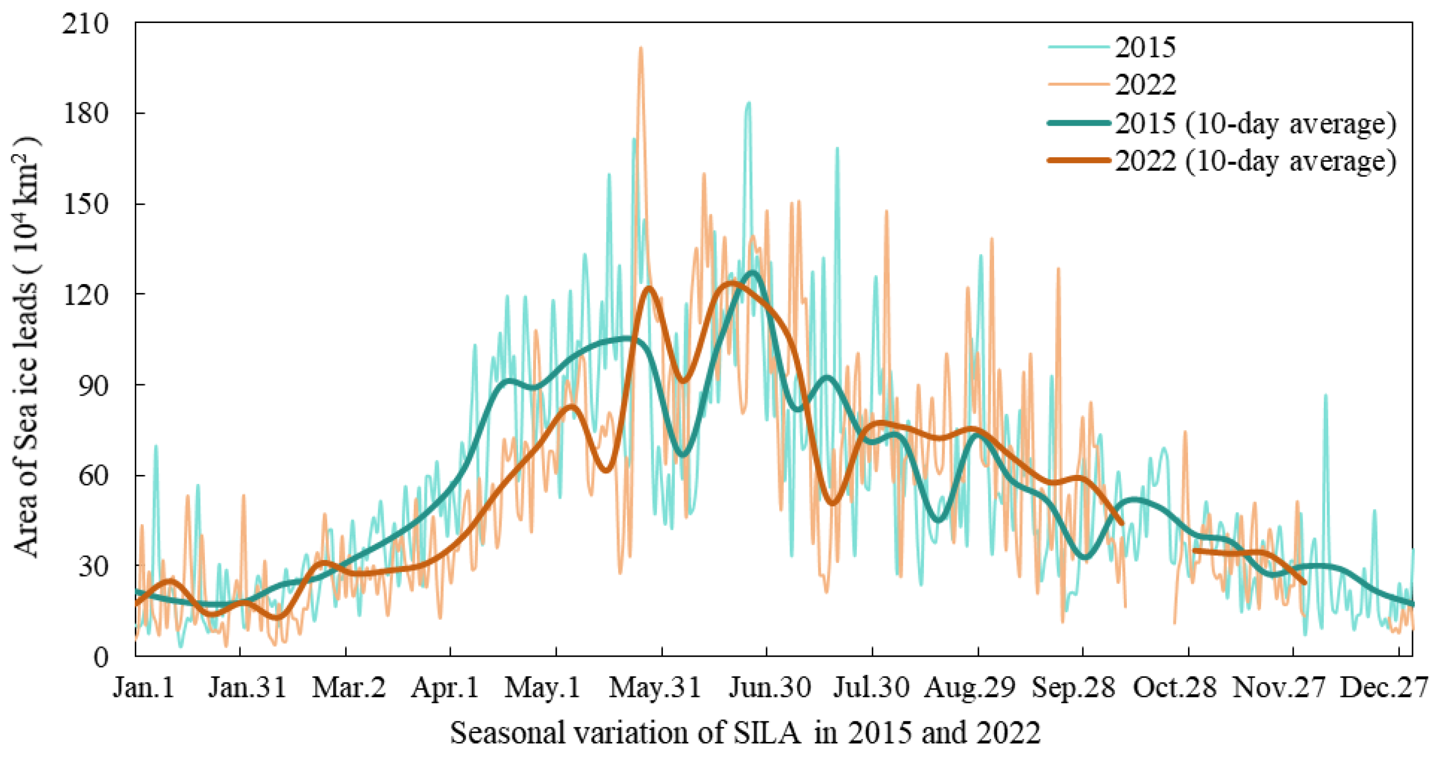
The daily sea ice lead areas (SILAs) for 2015 and 2022 were computed based on the daily leads map of Weddell Sea and are plotted in Figure 4 in a light line. And we smoothed it on a 10-day average window with a bold line. The variation in SILA in the Weddell Sea exhibited distinctive seasonal patterns, characterised by its lowest values during the summer months (January–March). Subsequently, there was a progressive increase, peaking during the fall (April–June), followed by a gradual decline during the winter (July–September) and spring (October–December). In 2015, the maximum SILA was observed on 25 June, reaching 1,834,174 km2, while the minimum occurred on 14 January, measuring 31,688 km2. Similarly, the minimum of 2022 also occurred in January, precisely on 27 January, with a value of 34,222 km2. The maximum of 2022 was recorded on 25 May, being a substantial value of 2,016,792 km2.
The difference in SILA between 2022 and 2015 was evident. Specifically, from January to May, the SILA of 2022 was lower than that of 2015. However, in June, the SILA of 2022 surpassed that of 2015, after which, on different dates, there was no discernible trend in the SILA differences. From an overarching perspective, the SILA in the Weddell Sea during 2022 remained below that of 2015.
3.2. Variation in SILA in the Latitudinal and Longitudinal Directions
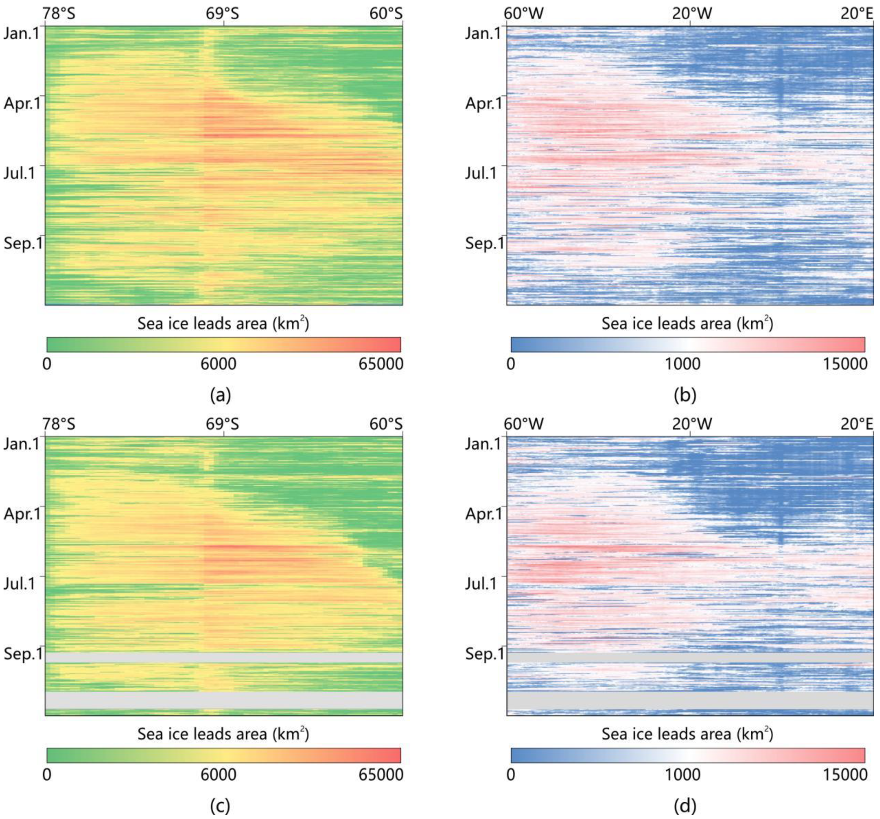
Since the study area focused on 60°W to 20°E and 60°S to 80°S, we summed the daily lead maps along the longitude and latitude directions with an interval of 0.25° to study the spatial distribution characteristics of SILA at different time periods. The resulting values were used as the X-axis, while the dates were used as the Y-axis to plot Figure 5.
In view of the overall situation, the characteristics of the SILA in 2015 and 2022 exhibited concordance in both directions. Along the zonal axis, the SILA is predominantly concentrated within the latitudinal band, spanning 70°S to 78°S in the entire year, which means that SIL were found more in higher latitudes. Meanwhile, within the latitudinal band spanning 60°S to 70°S, the variation trend of SILA shows an ascending trajectory from January to July, followed by a gradual descent from July to December, which aligns closely with the depiction in Figure 4. The results reveal that, in the latitude dimension, SILA variations in lower-latitude regions were more significantly influenced by seasonal factors.
Likewise, along the meridional axis, the SILA is primarily concentrated within the longitudinal range of 60°W to 30°W in the entire year, which indicates that SILs were more prevalent in the West Weddell Sea. Within the longitudinal range spanning 30°W to 20°E, the variation of the SILA also showed a similar trend as in Figure 4. This observation elucidates that the fluctuations of the SILA within the East Weddell Sea region were predominantly influenced by seasonal dynamics.
3.3. Spatial Distribution of Sea Ice Leads
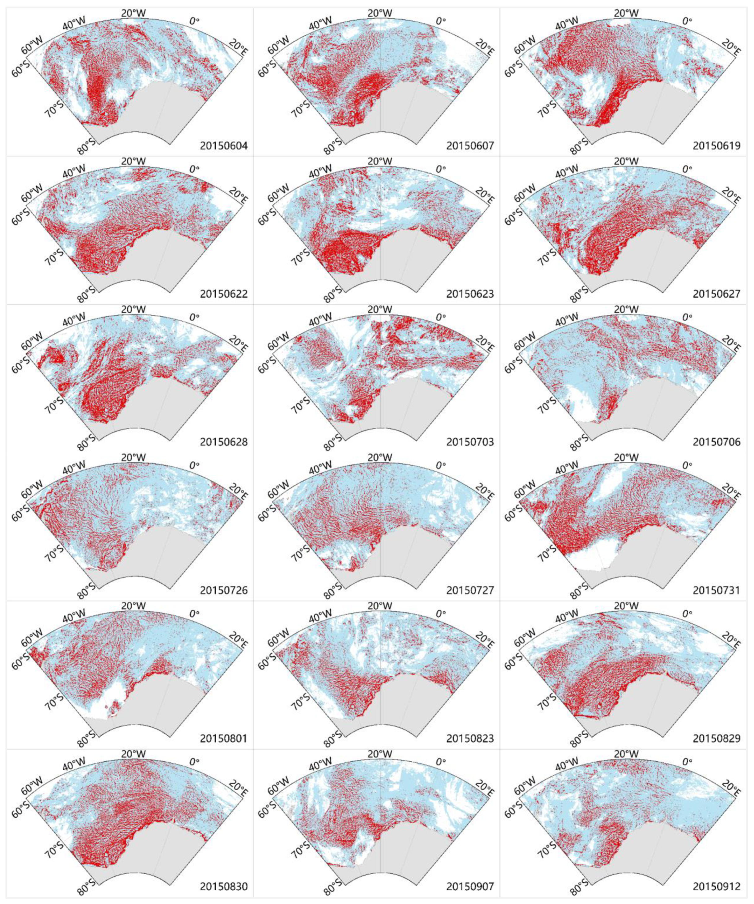
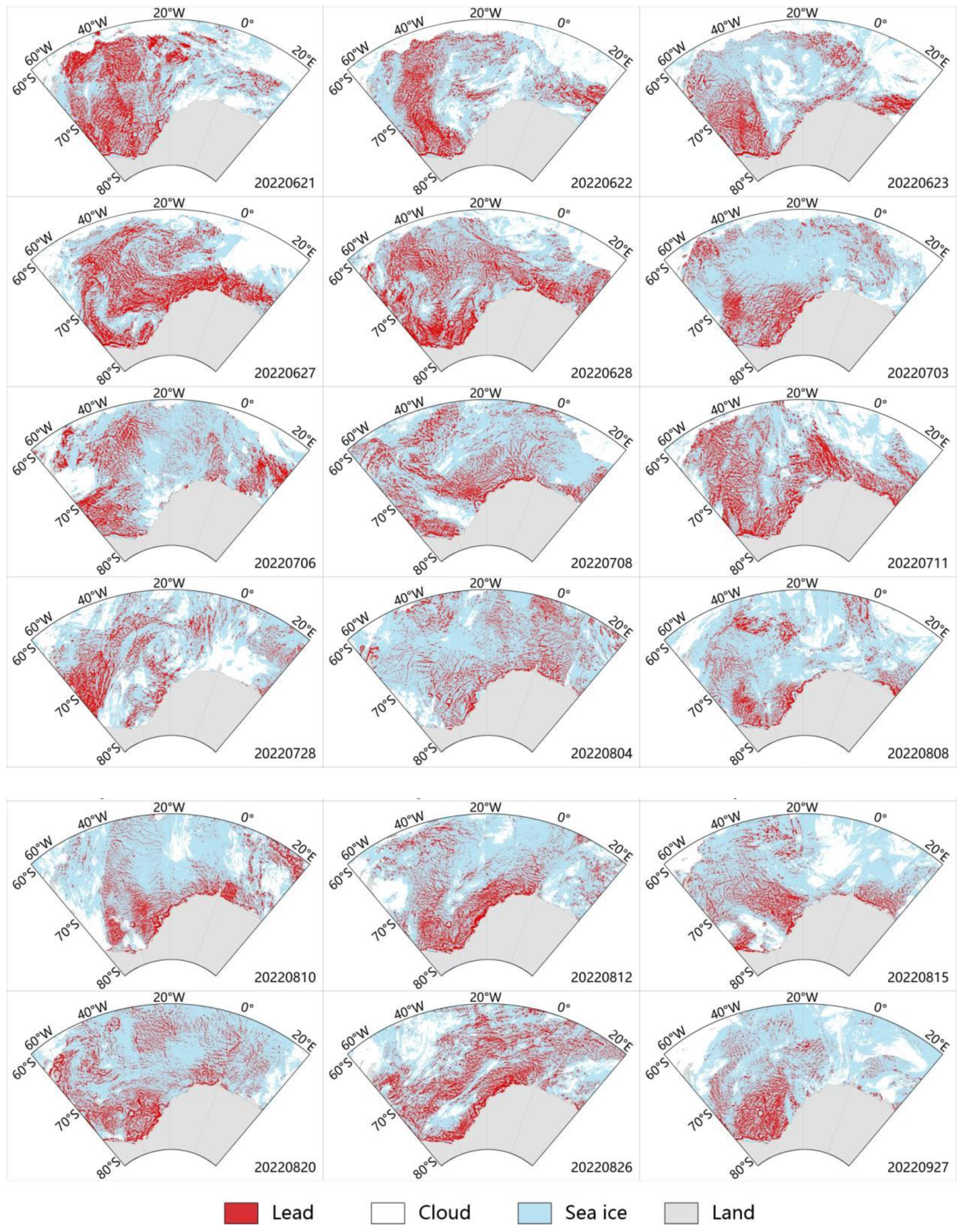
It is evident from Figure 4 that the SILA in the Weddell Sea was greater during the period spanning from June to September, compared to other months. Considering the potential influence of cloud cover on the identification of leads using MODIS data, we manually chose dates during the months of June to September for the years 2015 and 2022 when cloud cover was relatively minimal. Due to the relatively random nature of cloud cover, the selected date intervals are not evenly spaced. The spatial distribution maps of daily leads in the Weddell Sea for these selected dates are plotted in Figure 6. SILs were predominantly concentrated within the western Weddell Sea region proximate to the Antarctic Peninsula, whereas their distribution near the Queen Maud Land sector of the Antarctic remained comparatively sparse. This spatial distribution pattern bore resemblance to WSBW distribution characteristics influenced by WG [23,24]. Along the coastal regions, there was a pronounced increase in the number and density of SILs compared to offshore areas. The distribution characteristics align with the findings of Reiser et al. (2019) [34]. This observation may potentially signify a correlation between the distribution of leads and factors such as the density of WSBW, seafloor topography, and depths of the sea.
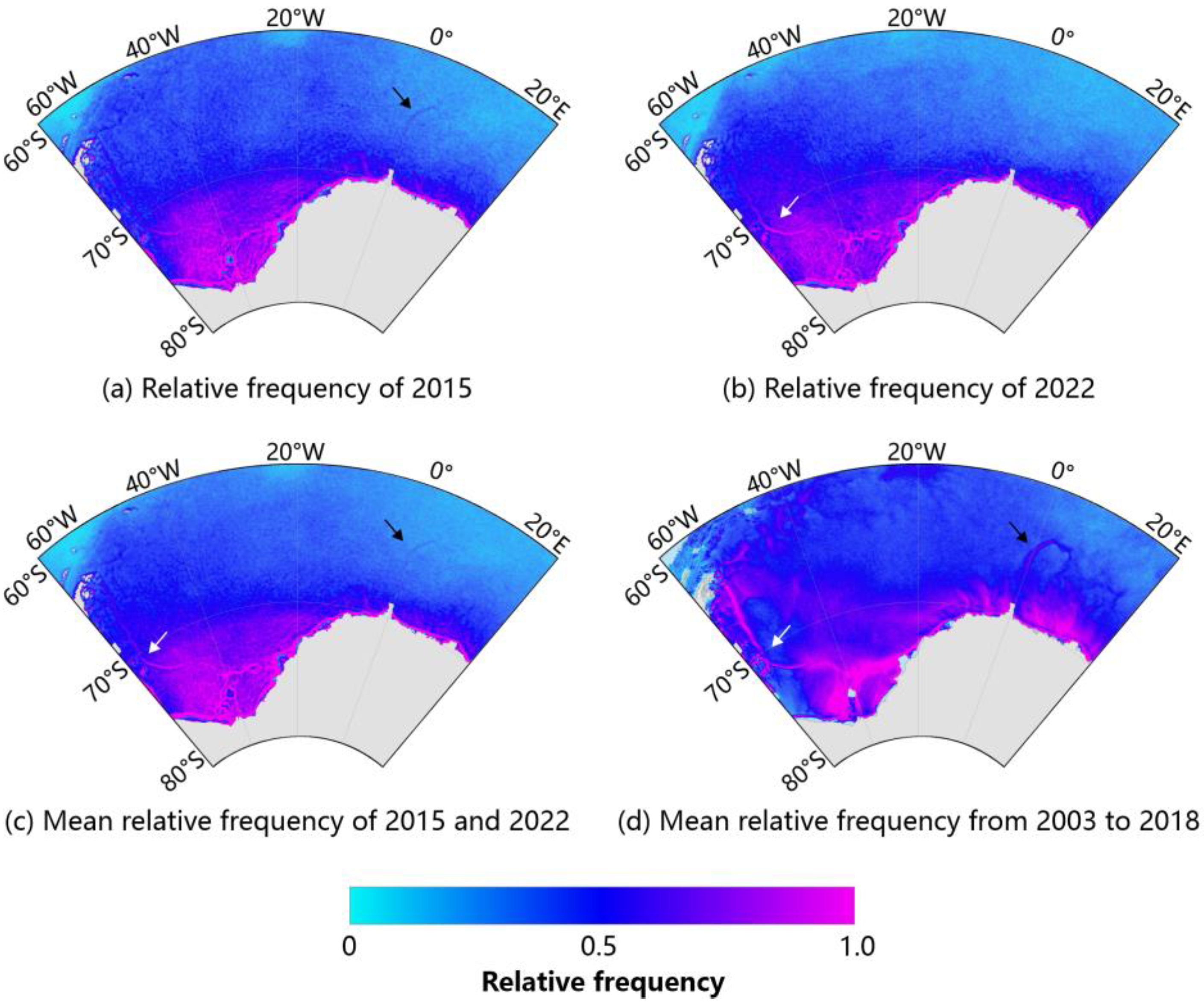
Reiser et al. (2020) [21] released long-term relative SIL frequency data of the Antarctic for the months of April to September spanning from 2003 to 2019 on Pangaea (https://doi.pangaea.de/10.1594/PANGAEA.917588 (27 November 2023)). In order to maintain temporal consistency, we selected daily SIL maps from April to September for both 2015 and 2022 and summed and averaged these maps to calculate relative frequency. We acquired the dataset from Pangaea and conducted a spatial cropping procedure tailored to our study area. For the purpose of enabling comparison, we normalized the frequency, and the results are illustrated in Figure 7.
Although our data differed in terms of years to Reiser’s dataset; notably, consistency was evident here after the mean and normalization processing. The black arrow in Figure 7a,c,d indicates the Maud Rise, which is an oceanic plateau, rising at its shallowest to depths of about a 1000 m. And the white arrow in Figure 7b–d indicates the Weddell Sea Polynya. According to Reiser et al. (2020) [21], the relative SIL frequency is pronounced in association with the shelf break and seabed ridges.
4. Discussion
4.1. Correlation Analysis with Thermodynamic and Kinetic Factors
Given that SILs serve as pivotal conduits for material and energy exchange between the atmosphere and the ocean and emerge because of sea ice dynamics, the distribution characteristics of leads are intricately intertwined with a multitude of influencing factors. From a thermodynamic perspective, elevated air temperatures induce the melting of sea ice, resulting in a reduction in its thickness, thereby rendering it more susceptible to fracturing and the formation of leads. Moreover, considering the kinetic aspect, fluctuations in sea level pressure contribute to variations in wind speed at the sea surface. Increased wind velocity accelerates sea ice motion, and, likewise, higher ocean current speeds lead to swifter sea ice movements, consequently promoting the generation of a greater number of leads.
In the realm of research pertaining to Arctic sea ice, Richter-Menge et al. (2002) [35] identified wind as a primary dynamic factor influencing ice deformation while investigating sea ice stresses in the Arctic under winter conditions. The interplay between wind and ocean currents collectively determines the direction of sea ice movement. Additionally, Lewis and Hutchings (2019) [36] observed a correlation between sea ice motion in the Beaufort Sea and the anticyclonic movement of the Beaufort Gyre, with the seasonal distribution of leads typically following the seasonal position of the Beaufort High. Consequently, to explore whether the causative factors for the formation of SILs in the Antarctic and Arctic exhibit similarities, we opted to study the same influencing factors.
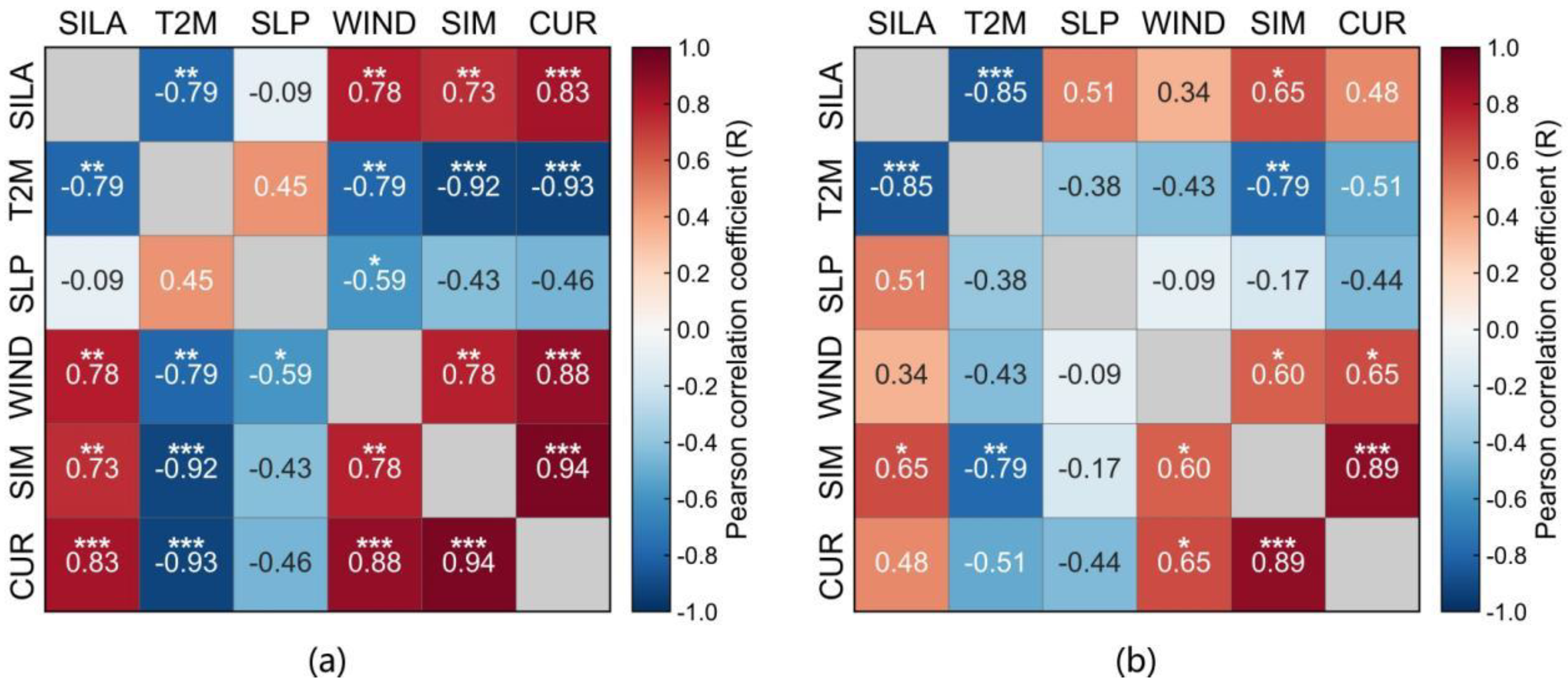
We integrated the ERA5 reanalysis product, including 2 m air temperature, 10 m wind speed, and sea level pressure, alongside sea ice motion vector data from NSIDC and ocean current data from the CFSR reanalysis product with SILA results mentioned in Section 3 and computed the correlation between the monthly means of each factor for the years 2015 and 2022 (Figure 8).
In 2015, the monthly mean SILA exhibited statistically significant negative correlations with the 2 m air temperature (p < 0.01), yielding a correlation coefficient of −0.79. Furthermore, the SILA demonstrated statistically significant positive correlations with 10 m wind speed and sea-ice motion velocity (p < 0.01), achieving correlation coefficients of 0.78 and 0.73, respectively. Additionally, the SILA exhibited a statistically significant positive correlation with ocean current speed (p < 0.001), yielding a correlation coefficient of 0.83. In 2022, the monthly mean SILA continued to display a statistically significant negative correlation with the 2 m air temperature (p < 0.001), with a notably strengthened correlation coefficient of −0.85. It maintained a statistically significant positive correlation with sea ice movement speed (p < 0.05), with a correlation coefficient of 0.65.
Figure 8 also illustrates a strong correlation between sea ice motion velocity, wind speed, and current velocity. In 2015, the correlation coefficient between sea ice motion velocity and wind speed was 0.78 (p < 0.01), while the correlation with current velocity was even stronger at 0.94 (p < 0.001). Comparatively, in 2022, the correlation coefficient between sea ice motion velocity and wind speed was 0.60 (p < 0.05), and with current velocity, it remained robust at 0.89 (p < 0.001). Notably, this suggested that the influence of current speed on sea ice motion velocity is more pronounced than that of wind speed.
A noteworthy question emerged here concerning the pronounced negative correlation between the SILA and the 2 m air temperature. Contrary to findings in Arctic SIL studies, which has been concluded that the heat released through leads contributes to a temperature increase [13]. That is to say, it implies a positive correlation between the SILA and air temperature. The divergent outcomes observed in the Antarctic and Arctic might be attributed to distinct factors. Firstly, conclusions drawn from the positive correlation between temperature and SILA in the Arctic region are subject to stringent limitations, as their study is restricted to clear sky conditions during a polar night. Secondly, the climates and marine environments of the Antarctic and Arctic greatly differ, and findings from Arctic sea ice research might not be applicable to the Antarctic.
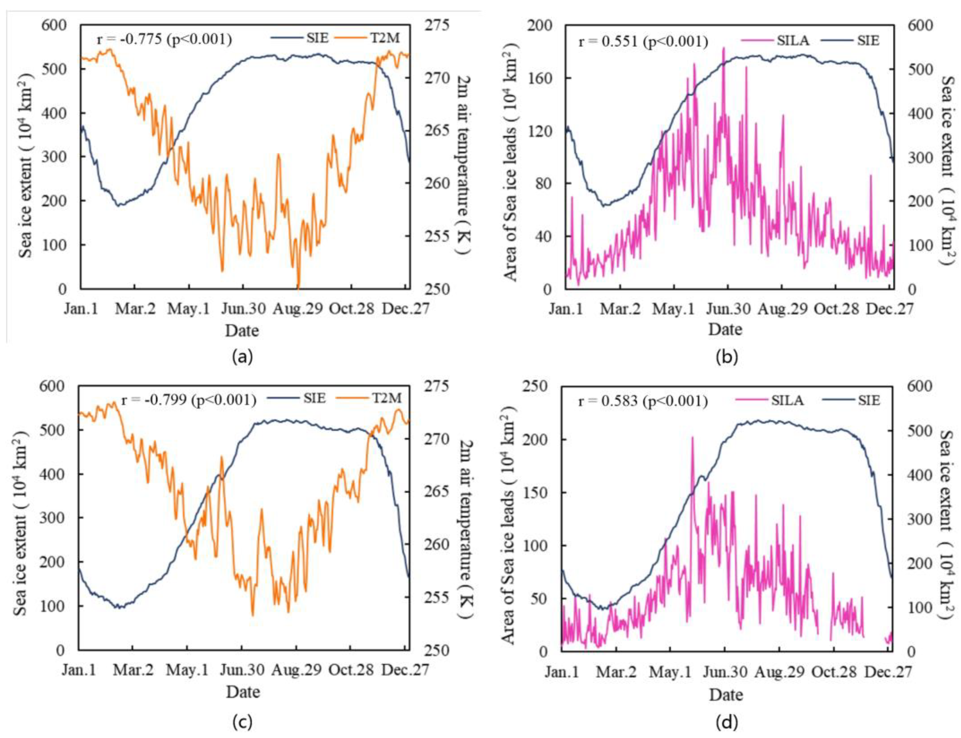
The current research on the correlation between SILs in the Southern Ocean and air temperatures remains rare, and we found it challenging to explain the significant negative correlation observed in Figure 8. In an attempt to unravel this phenomenon, we tried to investigate from the perspective of sea ice extent (SIE) as a bridging variable. Thus, we utilised sea ice concentration data from the University of Bremen to compute daily mean SIEs in the Weddell Sea for the years 2015 and 2022 and calculated the correlation between them and air temperature, as depicted in Figure 9a,c. The results revealed a notably negative correlation between them. Afterwards, we speculated that if there exists a strong positive correlation between the SIE and SILA, perhaps the negative correlation between temperature and leads is mediated by SIE serving as a bridging variable. Therefore, we proceeded to calculate the correlation coefficient between SIE and SILA, as illustrated in Figure 9b,d. The result indicated a relatively low correlation between them. Henceforth, we contended that SIE may not serve as a bridging variable to elucidate the correlation issues between SILA and air temperatures. The reasons pertaining to this matter need further investigation.
When coupled with the findings presented in Figure 8, it was evident that air temperature alone cannot elucidate the mechanisms governing the changes in leads on a broad spatial scale. However, this does not preclude the possibility of interactions between temperature and lead changes, which may require investigations at finer spatial and temporal resolutions. Notably, the results in Figure 8 underscore that the emergence of SILs is closely associated with dynamic factors such as wind field, sea ice motion, and ocean currents. This implies that leads serve as a direct manifestation of sea ice motion.
4.2. Spatial Correlation Analysis with Wind, Sea Ice Motion and Ocean Currents
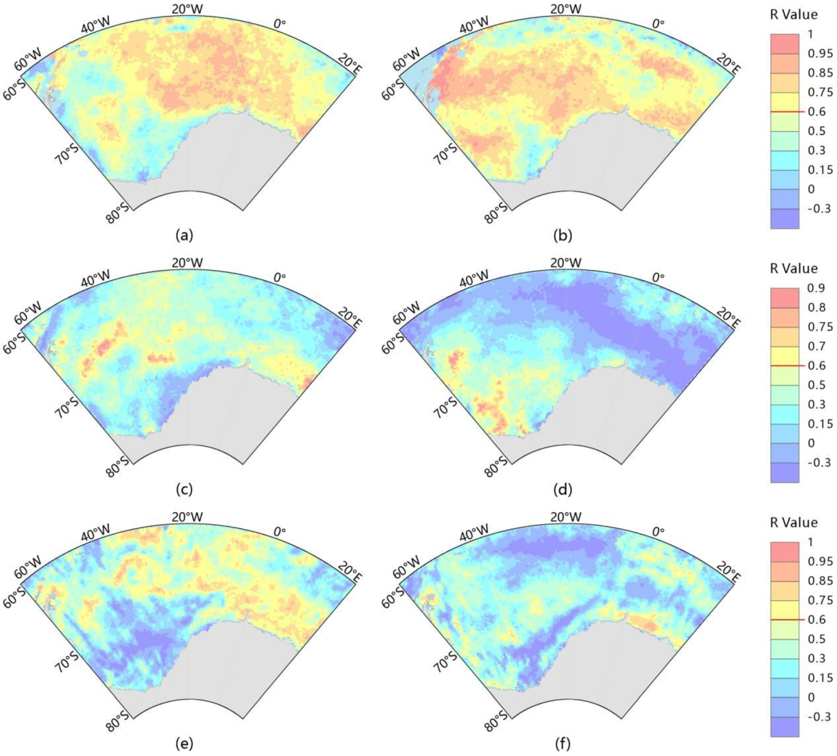
To investigate the relationship between leads distribution and sea ice motion, wind field, and ocean current within the Weddell Sea, we harmonised the resolution of daily leads maps, wind field data, and current data with that of the sea ice motion data (25 km). Then, we utilised monthly mean maps to assess the spatial correlations between the SILA and the velocity of sea ice motion, wind speed, and current speed for 2015 and 2022, and we depict the results in Figure 10.
In Figure 10a,b, it is obvious that in both 2015 and 2022, the correlation coefficients between the SILA and sea ice motion velocity in the vast majority of the Weddell Sea were above 0.75, albeit with slight variations in spatial distribution. In 2015, high-correlation regions were predominantly concentrated between 60°S and 70°S and spanned from 40°W to 20°E. In contrast, in 2022, notable correlation coefficients were primarily near the Antarctic Peninsula, the Ronne Ice Shelf, and the Coats Land region, with offshore regions displaying decreased correlation coefficients compared to 2015.
Comparing Figure 10c,d, in 2015, areas with a correlation coefficient above 0.7 between the SILA and 10 m wind speed were primarily in the Weddell Abyssal Plain and the Haakon VII Sea, concentrated within the latitudinal band of 60°S to 70°S. This result is consistent with the findings of Holland and Kwok (2012) [37], who studied the correlation between Antarctic sea ice drift and wind. They found a strong correlation between sea ice drift speed and wind speed in the Weddell Sea central area, while the correlation in coastal regions was relatively low. The low correlation in coastal areas is typically associated with convergent ice motion or flow near the coastline, where internal stresses are higher. As for 2022, regions exhibiting a correlation coefficient above 0.7 were mostly near the Antarctic Peninsula and the Ronne Ice Shelf, within latitudes 65°S to 70°S and longitudes 60°W to 40°W. Overall, the correlation coefficient for 2022 was lower than that for 2015, with a notably high negative correlation in the Eastern Weddell Sea.
As depicted in Figure 10e,f, in 2015, the regions within the Weddell Sea exhibiting a correlation coefficient of 0.75 or higher between the SILA and the ocean current velocity were primarily the Weddell Abyssal Plain and the Haakon VII Sea, spatially concentrated between 60°S to 70°S and 0° to 20°E. In contrast, by 2022, the areas where the correlation coefficient exceeded 0.75 were mostly near the Antarctic Peninsula and the Haakon VII Sea. Spatially, these areas were concentrated between 60°S to 75°S, 60°W to 40°W, and 0° to 20°E. Notably, the overall correlation coefficient for 2022 was lower than that for 2015, with a high negative correlation observed in the region spanning from 40°W to 20°W.
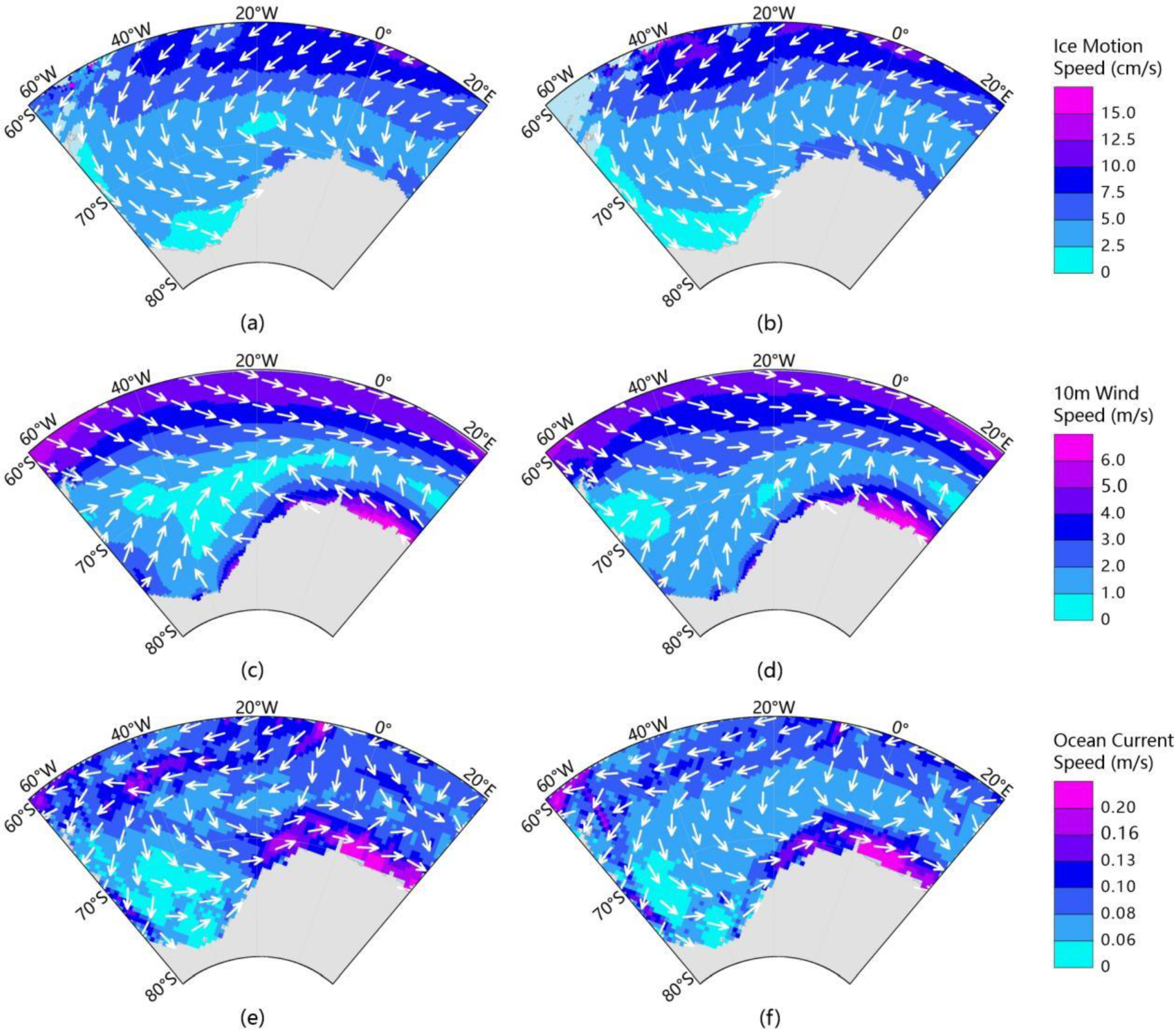
Annual mean sea ice motion velocity and direction maps for 2015 and 2022, along with annual mean wind speed and wind direction maps, as well as annual mean ocean current speed and current direction maps, were calculated and plotted based on sea ice motion data, 10 m wind field data, and ocean current data, as depicted in Figure 11.
A comparison of Figure 11a,b revealed that within the region spanning 60°W to 40°W and 60°S to 65°S, the sea ice motion speed in 2022 surpassed that of 2015. This difference likely contributed to the pronounced correlation observed between the SILA and sea ice motion in the same region shown in Figure 10b. Conversely, the notable correlation within the 40°W to 10°W range in both 2015 and 2022 could be attributed to eddies in the sea ice motion direction within this zone, and sea ice alterations in speed and direction within this region resulted in leads formation. The elevated sea ice motion velocity along the nearshore region of the Weddell Sea, ranging from 0° to 20°E, as depicted in Figure 11a,b, aligned with the zone displaying heightened correlation coefficients, as shown in Figure 10a,b.
When comparing Figure 10c and Figure 11c, it became evident that wind speeds exhibited greater magnitudes in the nearshore sector of the Weddell Sea in 2015, specifically within the longitudinal span of 0 to 20°E. This phenomenon was concomitant with correlation coefficients between the SILA and wind speed that surpassed the 0.7 threshold. A distinct core of diminished wind speeds materialised within the longitude range of 30°W to 20°W, characterised by prevailing westerly winds along the latitudinal axis; thus, this region also showed a heightened correlation between the SILA and wind speeds. Figure 11d conspicuously illustrates the presence of a low wind speed centre in the Weddell Sea during 2022, situated proximate to the Antarctic Peninsula within the nearshore domain, which might be a factor contributing to an elevated correlation between the SILA and wind speed in 2022 within this geographical expanse, as depicted in Figure 10d.
As depicted in Figure 11e, the current velocity in the region south of 70°S within the Weddell Sea, proximate to the Antarctic Peninsula and the Ronne Ice Shelf, exhibited lower values in 2015. This corresponded to a diminished correlation between the current speeds and SILA within this specific geographical range, which is shown in Figure 10e. The current velocity within the Weddell Sea sector near the Antarctic Peninsula and the Haakon VII region was relatively higher in both 2015 and 2022 (Figure 11e,f), which aligned with a higher correlation coefficient value between the current speeds and SILA within this geographical zone, as shown in Figure 10e,f.
4.3. Cloud Cover Effect
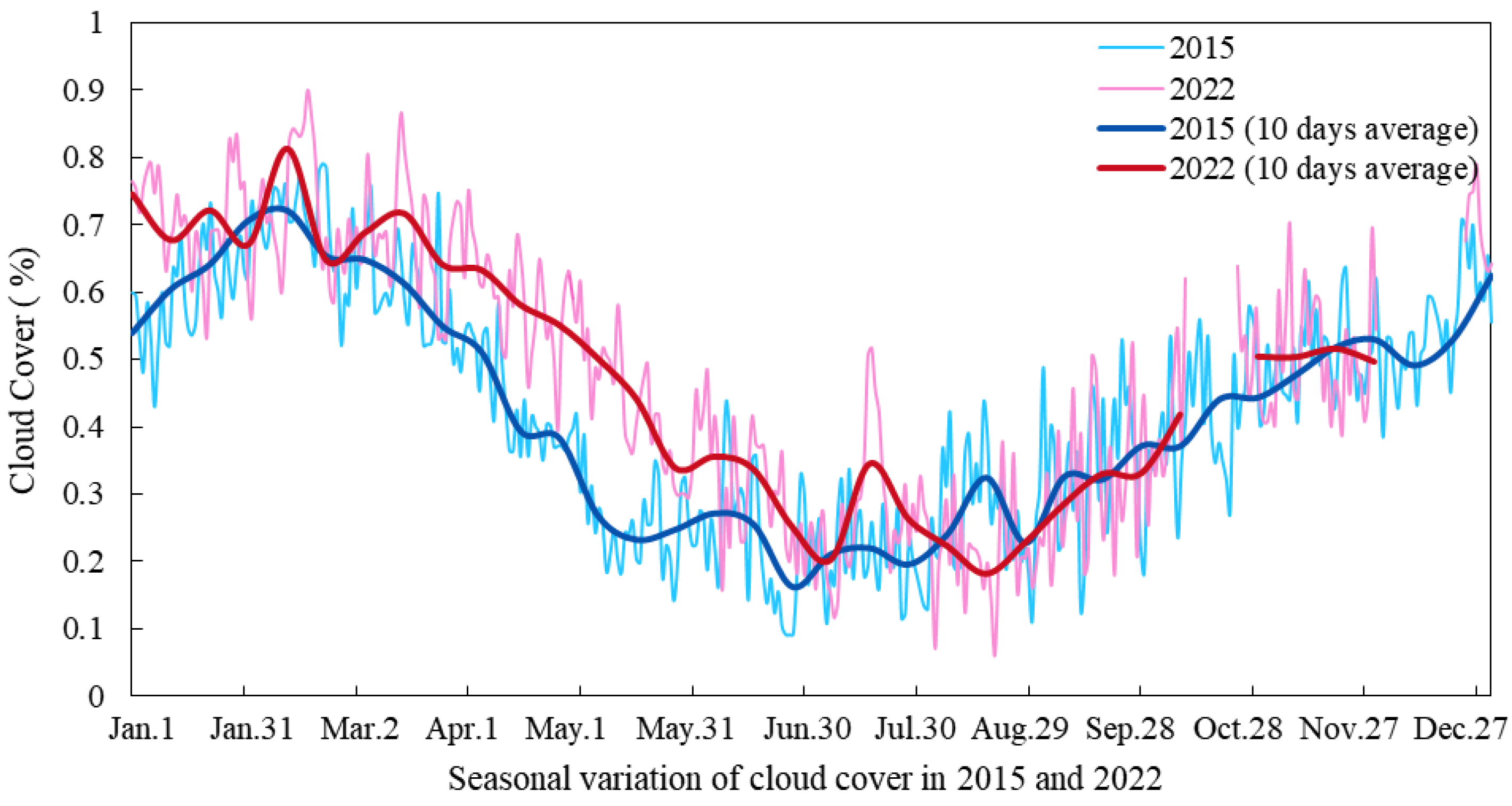
Given that the identification of leads critically depends on the cloud cover conditions prevailing in the local overhead atmosphere, the daily average cloud cover of the study area was calculated based on the optimised MOD35 product, which was used to assess the imaging conditions, image quality, and impact on leads extraction from MODIS imagery.
The temporal variation in cloud cover in the Weddell Sea, as illustrated in Figure 12, revealed that cloud cover in 2022 significantly surpassed that in 2015 during the period from January to July, and from August to September, the cloud cover in 2022 was slightly lower than that in 2015. Overall, the daily cloud cover over the Weddell Sea in 2022 exceeded that in 2015. This circumstance might potentially account for the comparatively diminished correlation between leads, wind speeds, and current velocities in Figure 8b for 2022.
In addition, we found in Figure 12 that there was a declining trend of cloud cover from January to June, followed by a subsequent increase from July to December, which contrasted with the trend of SILA variation. This implied that a higher cloud cover was associated with poorer MODIS imaging conditions and lower image quality, ultimately leading to the reduced identification of SILA. The finding correspondingly brought scepticism that the seasonality of the SILA might be the function of the cloud-free area of an image.
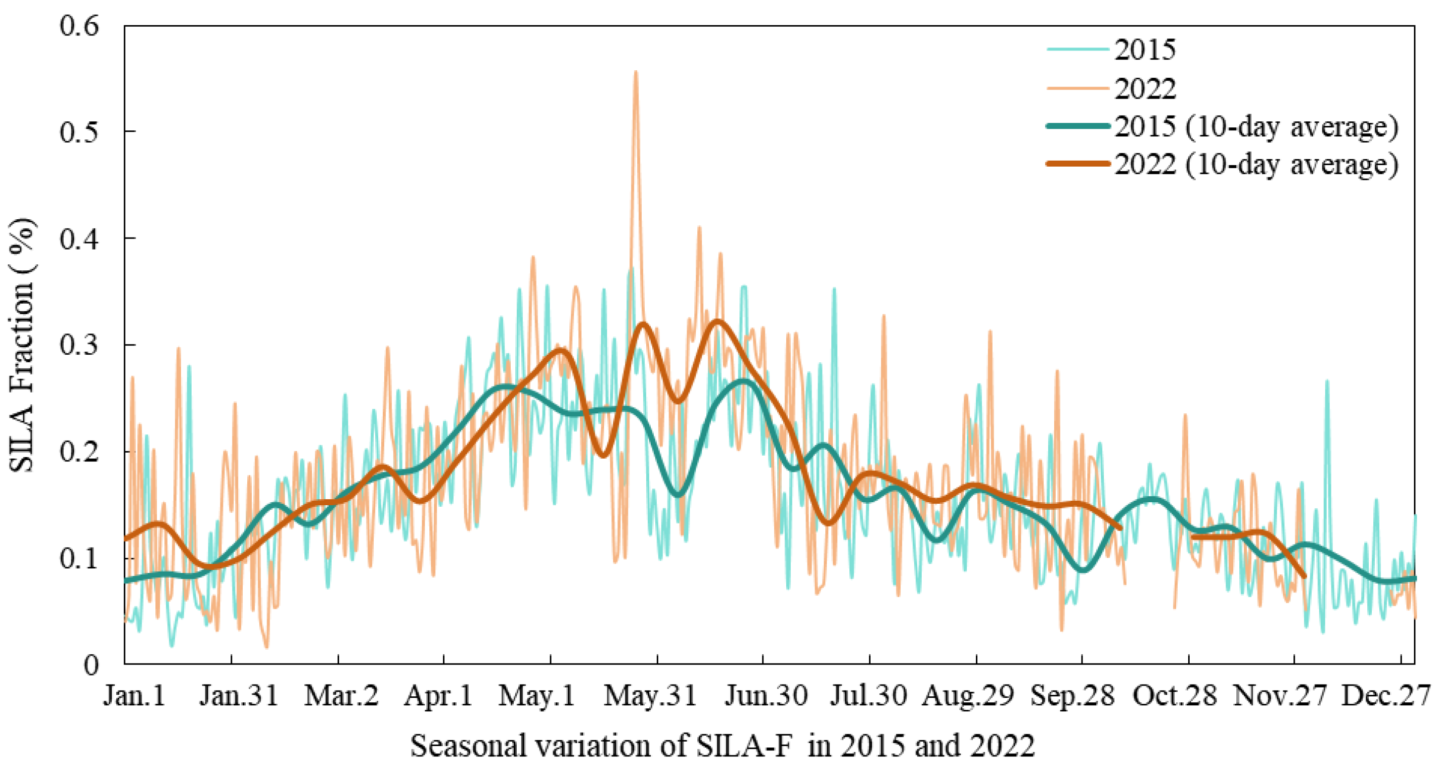
In order to assess the variation trends of the SILA while minimizing the impact of clouds, we proposed the “sea ice leads area fraction (SILA-F)”, which is defined as
where WSA is the area of the Weddell Sea, SILA is the area of sea ice leads, CA is the area of cloud coverage.
SILA-F = SILA/(WSA − CA)
5. Conclusions
Over the years, the changing trends in Antarctic sea ice have exhibited significant differences from those in the Arctic. While the sustained reduction of the Arctic sea ice has been widely attributed to global climate warming, Antarctic sea ice has also shown a diminishing trend in recent years. SILs serve as a crucial window for oceanic and atmospheric heat exchange, which have been extensively investigated in the Arctic, whereas studies related to these features in the Antarctic are comparatively scarce. In addition, the Weddell Sea has emerged as a pivotal region associated with the recent decline in Antarctic sea ice. We posit that studying the distribution characteristics and influencing factors of SILs in the Weddell Sea might be a foundation for understanding the reasons behind the reduction of the Antarctic sea ice.
In this study, a workflow for generating daily SIL distribution maps in the Weddell Sea was devised. This workflow involved an initial step of IST computation using MOD02 products, followed by the optimisation of MOD35 products. After cloud mask processing, daily lead maps were generated through the application of the iterative threshold method and raster-mosaic technique. The daily lead maps for 2015 and 2022 were obtained based on the workflow, and via the analysis of spatiotemporal variations in daily SILAs, it was found that SILA fluctuations in the Weddell Sea exhibited pronounced seasonality. During the summer (January to March), the SILA displayed a low value and then increased over time, reaching its maximum extent during the autumn season (April to June). Thereafter, it progressively diminished during the winter (July to September) and spring (October to December) months. The latitudinal extent of the larger SILA in the Weddell Sea was predominantly concentrated within the range of 66°S to 70°S, while the longitudinal extent of the larger SILA was primarily concentrated between 60°W and 30°W. An analysis of daily spatial distribution, focusing on dates characterised by lower cloud cover, revealed that the distribution of leads was mostly concentrated in the West Weddell Sea region proximate to the Antarctic Peninsula, whereas relatively fewer leads were observed near the Queen Maud Land area. In particular, the coastal regions exhibited a higher density of leads compared to offshore areas.
Afterwards, an exploration of the relationships between the formation of the SILA and meteorological and hydrological parameters, including air temperature, sea-level pressure, wind speed, sea ice motion velocity, and ocean current velocity, was conducted. The results indicated a close correlation between the SILA and the velocity of sea ice motion, with correlation coefficients of 0.73 in 2015 and 0.6 in 2022. Through an examination of the spatial correlation between the SILA and sea ice motion velocity, it was observed that in 2015, regions with a high correlation were concentrated between 60°S and 70°S and between 40°W and 20°E. In 2022, areas with high correlation coefficients were primarily situated near the Antarctic Peninsula, the Ronne Ice Shelf, and Coats Land, while offshore regions exhibited a decreased correlation coefficient compared to 2015. This distribution pattern corresponded to the spatial distribution of sea ice motion speed and direction in the Weddell Sea in 2015 and 2022.
Various satellite remote sensing datasets have distinct characteristics. SIL identification based on MODIS data can be susceptible to the distribution of cloud cover, while SAR data can effectively mitigate the impact of clouds on leads detection. However, its spatial coverage is limited and discontinuous, which hinders the exploration of long-term, large-scale SIL distribution patterns. In the future, it is advisable to combine diverse datasets to facilitate prolonged, high-resolution analyses of large-scale regions. This study will enhance our comprehension of the characteristics of Antarctic SIL, enabling a more profound interpretation of the interplay between the Antarctic climate–ocean system and the evolving trends in global climate change.
Author Contributions
Conceptualization, X.P. and Q.J.; methodology, M.Q. and Y.W.; software, Y.W.; validation, Y.W. and F.Z.; formal analysis, Y.W. and Z.Y.; investigation, Y.W.; resources, Y.W. and M.C.; data curation, Y.W. and B.H.; writing—original draft preparation, Y.W.; writing—review and editing, X.P., Q.J., M.Q., Y.W. and M.C.; visualization, Y.W. and M.C.; supervision, X.P. and Q.J.; project administration, X.P. and Q.J.; funding acquisition, X.P., Q.J. and M.Q. All authors have read and agreed to the published version of the manuscript.
Funding
This research was funded by the National Natural Science Foundation of China, grant number 42076235, and the National Natural Science Foundation of China, grant number 42206259.
Data Availability Statement
Data are contained within the article.
Conflicts of Interest
The authors declare no conflict of interest.
References
- Simmonds, I.; Wu, X. Cyclone Behaviour Response to Changes in Winter Southern Hemisphere Sea-Ice Concentration. Q. J. R. Met. Soc. 1993, 119, 1121–1148. [Google Scholar] [CrossRef]
- Parkinson, C.L. A 40-y Record Reveals Gradual Antarctic Sea Ice Increases Followed by Decreases at Rates Far Exceeding the Rates Seen in the Arctic. Proc. Natl. Acad. Sci. USA 2019, 116, 14414–14423. [Google Scholar] [CrossRef]
- Parkinson, C.L.; Cavalieri, D.J. Antarctic Sea Ice Variability and Trends, 1979–2010. Cryosphere 2012, 6, 871–880. [Google Scholar] [CrossRef]
- Comiso, J.C.; Gersten, R.A.; Stock, L.V.; Turner, J.; Perez, G.J.; Cho, K. Positive Trend in the Antarctic Sea Ice Cover and Associated Changes in Surface Temperature. J. Clim. 2017, 30, 2251–2267. [Google Scholar] [CrossRef]
- Schlosser, E.; Haumann, F.A.; Raphael, M.N. Atmospheric Influences on the Anomalous 2016 Antarctic Sea Ice Decay. Cryosphere 2018, 12, 1103–1119. [Google Scholar] [CrossRef]
- Eayrs, C.; Li, X.; Raphael, M.N.; Holland, D.M. Rapid Decline in Antarctic Sea Ice in Recent Years Hints at Future Change. Nat. Geosci. 2021, 14, 460–464. [Google Scholar] [CrossRef]
- Turner, J.; Holmes, C.; Caton Harrison, T.; Phillips, T.; Jena, B.; Reeves-Francois, T.; Fogt, R.; Thomas, E.R.; Bajish, C.C. Record Low Antarctic Sea Ice Cover in February 2022. Geophys. Res. Lett. 2022, 49, e2022GL098904. [Google Scholar] [CrossRef]
- Jena, B.; Bajish, C.C.; Turner, J.; Ravichandran, M.; Anilkumar, N.; Kshitija, S. Record Low Sea Ice Extent in the Weddell Sea, Antarctica in April/May 2019 Driven by Intense and Explosive Polar Cyclones. Npj Clim. Atmos. Sci. 2022, 5, 19. [Google Scholar] [CrossRef]
- Turner, J.; Hosking, J.S.; Bracegirdle, T.J.; Marshall, G.J.; Phillips, T. Recent Changes in Antarctic Sea Ice. Phil. Trans. R. Soc. A 2015, 373, 20140163. [Google Scholar] [CrossRef]
- Miles, M.W.; Barry, R.G. A 5-year Satellite Climatology of Winter Sea Ice Leads in the Western Arctic. J. Geophys. Res. 1998, 103, 21723–21734. [Google Scholar] [CrossRef]
- Cabaniss, G.H. US-IGY Drifting Station Alpha, Arctic Ocean, 1957–1958. 1965. Available online: https://www.psu.edu/ (accessed on 27 November 2023).
- Maykut, G.A. Energy Exchange over Young Sea Ice in the Central Arctic. J. Geophys. Res. 1978, 83, 3646. [Google Scholar] [CrossRef]
- Lüpkes, C.; Vihma, T.; Birnbaum, G.; Wacker, U. Influence of Leads in Sea Ice on the Temperature of the Atmospheric Boundary Layer during Polar Night. Geophys. Res. Lett. 2008, 35, L03805. [Google Scholar] [CrossRef]
- Eisen, O.; Kottmeier, C. On the Importance of Leads in Sea Ice to the Energy Balance and Ice Formation in the Weddell Sea. J. Geophys. Res. 2000, 105, 14045–14060. [Google Scholar] [CrossRef]
- Lindsay, R.W.; Rothrock, D.A. Arctic Sea Ice Leads from Advanced Very High Resolution Radiometer Images. J. Geophys. Res. 1995, 100, 4533. [Google Scholar] [CrossRef]
- Willmes, S.; Heinemann, G. Pan-Arctic Lead Detection from MODIS Thermal Infrared Imagery. Ann. Glaciol. 2015, 56, 29–37. [Google Scholar] [CrossRef]
- Murashkin, D.; Spreen, G. Sea Ice Leads Detected From Sentinel-1 SAR Images. In Proceedings of the IGARSS 2019—2019 IEEE International Geoscience and Remote Sensing Symposium, Yokohama, Japan, 28 July 2019–2 August 2019; IEEE: Yokohama, Japan, 2019; pp. 174–177. [Google Scholar]
- Marcq, S.; Weiss, J. Influence of Sea Ice Lead-Width Distribution on Turbulent Heat Transfer between the Ocean and the Atmosphere. Cryosphere 2012, 6, 143–156. [Google Scholar] [CrossRef]
- Qu, M.; Pang, X.; Zhao, X.; Zhang, J.; Ji, Q.; Fan, P. Estimation of Turbulent Heat Flux over Leads Using Satellite Thermal Images. Cryosphere 2019, 13, 1565–1582. [Google Scholar] [CrossRef]
- Zhang, Y.; Cheng, X.; Liu, J.; Hui, F. The Potential of Sea Ice Leads as a Predictor for Summer Arctic Sea Ice Extent. Cryosphere 2018, 12, 3747–3757. [Google Scholar] [CrossRef]
- Reiser, F.; Willmes, S.; Heinemann, G. A New Algorithm for Daily Sea Ice Lead Identification in the Arctic and Antarctic Winter from Thermal-Infrared Satellite Imagery. Remote Sens. 2020, 12, 1957. [Google Scholar] [CrossRef]
- Muchow, M.; Schmitt, A.U.; Kaleschke, L. A Lead-Width Distribution for Antarctic Sea Ice: A Case Study for the Weddell Sea with High-Resolution Sentinel-2 Images. Cryosphere 2021, 15, 4527–4537. [Google Scholar] [CrossRef]
- Vernet, M.; Geibert, W.; Hoppema, M.; Brown, P.J.; Haas, C.; Hellmer, H.H.; Jokat, W.; Jullion, L.; Mazloff, M.; Bakker, D.C.E.; et al. The Weddell Gyre, Southern Ocean: Present Knowledge and Future Challenges. Rev. Geophys. 2019, 57, 623–708. [Google Scholar] [CrossRef]
- Zhou, S.; Meijers, A.J.S.; Meredith, M.P.; Abrahamsen, E.P.; Holland, P.R.; Silvano, A.; Sallée, J.-B.; Østerhus, S. Slowdown of Antarctic Bottom Water Export Driven by Climatic Wind and Sea-Ice Changes. Nat. Clim. Change 2023, 13, 701–709. [Google Scholar] [CrossRef]
- Kwok, R. Deformation of the Arctic Ocean Sea Ice Cover between November 1996 and April 1997: A Qualitative Survey. In IUTAM Symposium on Scaling Laws in Ice Mechanics and Ice Dynamics; Dempsey, J.P., Shen, H.H., Eds.; Solid Mechanics and Its Applications; Springer: Dordrecht, The Netherlands, 2001; Volume 94, pp. 315–322. ISBN 978-90-481-5890-4. [Google Scholar]
- Spreen, G.; Kaleschke, L.; Heygster, G. Sea Ice Remote Sensing Using AMSR-E 89-GHz Channels. J. Geophys. Res. Ocean. 2008, 113, C02S03. [Google Scholar] [CrossRef]
- Hoffman, J.; Ackerman, S.; Liu, Y.; Key, J. The Detection and Characterization of Arctic Sea Ice Leads with Satellite Imagers. Remote Sens. 2019, 11, 521. [Google Scholar] [CrossRef]
- Key, J.R.; Collins, J.B.; Fowler, C.; Stone, R.S. High-Latitude Surface Temperature Estimates from Thermal Satellite Data. Remote Sens. Environ. 1997, 61, 302–309. [Google Scholar] [CrossRef]
- Hall, D.K.; Key, J.R.; Case, K.A.; Riggs, G.A.; Cavalieri, D.J. Sea Ice Surface Temperature Product from MODIS. IEEE Trans. Geosci. Remote Sens. 2004, 42, 1076–1087. [Google Scholar] [CrossRef]
- Fraser, A.D.; Massom, R.A.; Michael, K.J. A Method for Compositing Polar MODIS Satellite Images to Remove Cloud Cover for Landfast Sea-Ice Detection. IEEE Trans. Geosci. Remote Sens. 2009, 47, 3272–3282. [Google Scholar] [CrossRef]
- Drusch, M.; Del Bello, U.; Carlier, S.; Colin, O.; Fernandez, V.; Gascon, F.; Hoersch, B.; Isola, C.; Laberinti, P.; Martimort, P.; et al. Sentinel-2: ESA’s Optical High-Resolution Mission for GMES Operational Services. Remote Sens. Environ. 2012, 120, 25–36. [Google Scholar] [CrossRef]
- Massonnet, F.; Guemas, V.; Fuckar, N.S.; Doblas-Reyes, F.J. The 2014 high record of Antarctic sea ice extent [in ‘‘Explaining Extremes of 2014 from a Climate Perspective’’]. Bull. Am. Meteor. Soc. 2015, 96, S163–S167. [Google Scholar] [CrossRef]
- Wang, Z.; Turner, J.; Wu, Y.; Liu, C. Rapid Decline of Total Antarctic Sea Ice Extent during 2014–16 Controlled by Wind-Driven Sea Ice Drift. J. Clim. 2019, 32, 5381–5395. [Google Scholar] [CrossRef]
- Reiser, F.; Willmes, S.; Hausmann, U.; Heinemann, G. Predominant Sea Ice Fracture Zones Around Antarctica and Their Relation to Bathymetric Features. Geophys. Res. Lett. 2019, 46, 12117–12124. [Google Scholar] [CrossRef]
- Richter-Menge, J.A.; McNutt, S.L.; Overland, J.E.; Kwok, R. Relating Arctic Pack Ice Stress and Deformation under Winter Conditions. J. Geophys. Res. 2002, 107(C10), 8040. [Google Scholar] [CrossRef]
- Lewis, B.J.; Hutchings, J.K. Leads and Associated Sea Ice Drift in the Beaufort Sea in Winter. JGR Ocean. 2019, 124, 3411–3427. [Google Scholar] [CrossRef]
- Holland, P.R.; Kwok, R. Wind-Driven Trends in Antarctic Sea-Ice Drift. Nat. Geosci. 2012, 5, 872–875. [Google Scholar] [CrossRef]

Figure 2.
Distribution of Sentinel-2 data used in this study (the label corresponds the serial number in Figure 3).
Figure 2.
Distribution of Sentinel-2 data used in this study (the label corresponds the serial number in Figure 3).

Figure 3.
Comparison of SILs detected from Sentinel-2 and MODIS.

Figure 4.
Temporal SILA variation in 2015 and 2022.

Figure 5.
The SILA of the Weddell Sea in the latitudinal and longitudinal directions, where (a,b) represent the latitudinal and longitudinal results of 2015, and (c,d) represent the latitudinal and longitudinal results of 2022. (Grey colour represents the missing data).
Figure 5.
The SILA of the Weddell Sea in the latitudinal and longitudinal directions, where (a,b) represent the latitudinal and longitudinal results of 2015, and (c,d) represent the latitudinal and longitudinal results of 2022. (Grey colour represents the missing data).

Figure 6.
Spatial distribution of the leads for the period of June to September in 2015 and 2022.


Figure 7.
Observed lead frequencies based on daily composites for the period of April to September, where (a,b) represent the relative frequency of 2015 and 2022, respectively, (c) represents the mean relative frequency of 2015 and 2022, and (d) represents the mean relative frequency from 2003 to 2019 according to Reiser’s dataset. The arrows indicate the similarity of the comparison.

Figure 8.
Correlation coefficients between factors in 2015 (a) and 2022 (b). (SILA: sea ice leads area, T2M: 2 m air temperature, SLP: mean sea level pressure, WIND: 10 m wind speed, SIM: sea ice motion speed, CUR: ocean current speed. * denotes a significance level of 0.05, ** denotes a significance level of 0.01 and *** denotes a significance level of 0.001).

Figure 9.
Changes in SIE and 2 m temperature in 2015 (a) and 2022 (c); changes in SIE and SILA in 2015 (b) and 2022 (d).
Figure 9.
Changes in SIE and 2 m temperature in 2015 (a) and 2022 (c); changes in SIE and SILA in 2015 (b) and 2022 (d).

Figure 10.
Spatial correlation between SILA and the velocity of sea ice motion (a), wind speed (c), and current speed (e) in 2015, and the right columns (b,d,f) are the corresponding factors in 2022. (The pixels with correlation coefficients (r) greater than 0.6 exhibit p values below 0.05).
Figure 10.
Spatial correlation between SILA and the velocity of sea ice motion (a), wind speed (c), and current speed (e) in 2015, and the right columns (b,d,f) are the corresponding factors in 2022. (The pixels with correlation coefficients (r) greater than 0.6 exhibit p values below 0.05).

Figure 11.
The speed and direction map of sea ice motion (a), wind field (c), and ocean current (e) in 2015, and the right columns (b,d,f) are the corresponding factors in 2022.
Figure 11.
The speed and direction map of sea ice motion (a), wind field (c), and ocean current (e) in 2015, and the right columns (b,d,f) are the corresponding factors in 2022.

Figure 12.
Temporal cloud cover variation in 2015 and 2022.

Figure 13.
Temporal lead fraction variation in 2015 and 2022.


Table 1.
Precision results of the comparison.
| Sensing Date (dd/mm/yyyy) | Product Name | Precision * |
|---|---|---|
| 9 March 2022 | S2B_MSIL1C_20220309T100059_N0400_R093_T25CDS_20220309T112924 | 94.24% |
| 17 March 2022 | S2B_MSIL1C_20220317T110249_N0400_R065_T23CNS_20220317T140318 | 87.06% |
| 18 March 2022 | S2B_MSIL1C_20220318T103149_N0400_R079_T25CDU_20220318T120424 | 88.98% |
| 23 March 2022 | S2B_MSIL1C_20220323T125859_N0400_R009_T21DVE_20220323T174633 | 93.12% |
| 5 September 2022 | S2B_MSIL1C_20220905T100059_N0509_R093_T26DPG_20230125T141937 | 87.29% |
| 31 October 2022 | S2B_MSIL1C_20221031T102139_N0400_R036_T26CMD_20221031T114320 | 80.33% |
| 10 November 2022 | S2B_MSIL1C_20221110T120239_N0400_R037_T22CDD_20221110T132417 | 85.08% |
| 18 November 2022 | S2B_MSIL1C_20221118T094019_N0400_R007_T24CWV_20221118T112152 | 81.21% |
* Precision = TP/(TP + FP), where TP, FP represent the cell numbers of true positives, false positives, respectively.
Disclaimer/Publisher’s Note: The statements, opinions and data contained in all publications are solely those of the individual author(s) and contributor(s) and not of MDPI and/or the editor(s). MDPI and/or the editor(s) disclaim responsibility for any injury to people or property resulting from any ideas, methods, instructions or products referred to in the content. |
© 2023 by the authors. Licensee MDPI, Basel, Switzerland. This article is an open access article distributed under the terms and conditions of the Creative Commons Attribution (CC BY) license (https://creativecommons.org/licenses/by/4.0/).
Share and Cite
MDPI and ACS Style
Wang, Y.; Ji, Q.; Pang, X.; Qu, M.; Cha, M.; Zhang, F.; Yan, Z.; He, B. Distribution Characteristics and Influencing Factors of Sea Ice Leads in the Weddell Sea, Antarctica. Remote Sens. 2023, 15, 5568. https://doi.org/10.3390/rs15235568
AMA Style
Wang Y, Ji Q, Pang X, Qu M, Cha M, Zhang F, Yan Z, He B. Distribution Characteristics and Influencing Factors of Sea Ice Leads in the Weddell Sea, Antarctica. Remote Sensing. 2023; 15(23):5568. https://doi.org/10.3390/rs15235568
Chicago/Turabian StyleWang, Yueyun, Qing Ji, Xiaoping Pang, Meng Qu, Mingxing Cha, Fanyi Zhang, Zhongnan Yan, and Bin He. 2023. "Distribution Characteristics and Influencing Factors of Sea Ice Leads in the Weddell Sea, Antarctica" Remote Sensing 15, no. 23: 5568. https://doi.org/10.3390/rs15235568
Note that from the first issue of 2016, this journal uses article numbers instead of page numbers. See further details here.