
A Radar Reflectivity Image Prediction Method: The Spatial MIM + Pix2Pix

1
School of Electrical and Information Engineering, Tianjin University, Tianjin 300072, China
2
School of Information Science and Engineering, Shandong Normal University, Jinan 250014, China
*
Author to whom correspondence should be addressed.
Remote Sens. 2023, 15(23), 5554; https://doi.org/10.3390/rs15235554
Submission received: 31 October 2023
/
Revised: 24 November 2023
/
Accepted: 26 November 2023
/
Published: 29 November 2023
(This article belongs to the Topic Radar Signal and Data Processing with Applications)
Abstract
:Radar reflectivity images have the potential to provide vital information on the development of convective cloud interiors, which can play a critical role in precipitation prediction. However, traditional prediction methods face challenges in preserving the high-frequency component, leading to blurred prediction results. To address this issue and accurately estimate radar reflectivity intensity, this paper proposes a novel reflectivity image prediction approach based on the Spatial Memory in Memory (Spatial MIM) networks and the Pix2Pix networks. Firstly, a rough radar reflectivity image prediction is made using the Spatial MIM network. Secondly, the prediction results from the Spatial MIM network are fed into the Pix2pix network, which improves the high-frequency component of the predicted image and solves the image blurring issue. Finally, the proposed approach is evaluated using data from Oklahoma in the United States during the second and third quarters of 2021. The experimental results demonstrate that the proposed approach yields more accurate radar reflectivity prediction images.
1. Introduction
In the field of meteorology, radar is a very effective piece of equipment [1,2,3,4,5]. It can provide data including reflectivity intensity, spectral width and velocity, which can provide powerful data support for weather prediction [6,7,8,9,10]. Based on radar data, meteorologists are able to observe the 3D structural features of near-surface cloud clusters. These 3D features can be used to identify and track cloud clusters. Based on the identification and tracking of the cloud clusters, the future trajectory of the cloud clusters can be forecast. The usual idea is to use traditional prediction methods or deep learning methods to process past moment reflectivity images and then forecast future reflectivity images. Following the completion of reflectivity images prediction, subsequent work such as precipitation particle class identification and precipitation forecasting can be performed. The accuracy of the reflectivity images prediction results is crucial for future work.
2. Related Work
Traditional radar image prediction methods can be divided into per-pixel forecasts [11,12,13,14] and convective cloud forecasts [15,16,17,18,19]. The Tracking of Radar Echo with Correlations (TREC) [11] is the classical method for per-pixel forecasts. This method calculates the direction of motion of each pixel and determines the speed of motion, which in turn leads to a full-image forecast. The optical flow method [20,21,22] builds on the idea of TREC. This method only uses a few pixels near the prediction pixel to calculate in the prediction process. This makes it difficult for prediction methods to cope with the complexity and variability of strong convective weather. The Thunderstorm Identification, Tracking, Analysis and Forecasting (TITAN) [15] method and the Storm Cell Identification and Tracking (SCIT) [16] method are classic methods based on convective cloud cluster prediction methods. These methods take convective cloud cluster as an object, track the convective cloud cluster and calculate the speed and direction of the cloud’s future motion. The prediction method based on convective cloud cluster also has its limitations. These methods forecast clouds as a whole. The change of internal structure and strength during the prediction process is not considered. Furthermore, there is no training process for these methods, and the forecasts of historical samples will not help the current moment forecasts.
Deep learning methods have developed rapidly in recent years [23,24,25]. These methods have been useful in strong convective monitoring and short-term prediction. Their application is therefore superior to traditional methods that rely on subjective experience and objective statistical features. Recurrent Neural Networks (RNN) [9,26] have significant advantages in processing time series data, and the method is widely used in video prediction. The addition of methods such as Long Short-Term Memory (LSTM) and Gated Recurrent Unit (GRU) to RNN networks allows more spatiotemporal information to be captured. Shi et al. [27] used an RNN model for the first time to forecast radar reflectivity images. The fully connected form of the state-to-state transition in the LSTM model was changed to a convolutional form. It can capture spatial information better and save computational resources effectively. Experimental results show a significant improvement of the method over the optical flow method in the field of short-time prediction. At the same time, it also shows that RNN models have great potential to solve this practical problem. Shi et al. [28] proposed the Trajectory GRU (TrajGRU) model based on the Convlstm. This model can learn the position change of natural motion and at the same time can better learn the spatiotemporal information of radar reflectivity images. Wang et al. [29] proposed a Predictive Recurrent Neural Network (PredRNN) where the memory states are no longer confined within each RNN unit but can be shifted in both horizontal and vertical directions. This method achieved excellent performance on radar datasets. Wang et al. [30] proposed the PredRNN++ network on the basis of the PredRNN network. This method alleviates the gradient disappearance problem by improving the LSTM with causal LSTM structure and adding Gradient Highway Units (GHU). Xie et al. [31] proposed the MIM network in order to address the problem of spatiotemporal non-stationarity. This method can better capture complex spatiotemporal non-stationarity through two cascaded self-updating memory modules while learning the changes in a continuous spatiotemporal context. Wang et al. [32] proposed an extrapolation model based on convolutional neural networks and generative adversarial networks in order to address the lack of small-scale details in the echoes. This model can better preserve the details in the forecast.
Compared with traditional methods, although the accuracy of radar image prediction method based on the neural network is higher, there is still room for improvement. Neural networks are trained by constructing a loss function that measures the difference between the predicted and true values of the network. As training progresses, the loss function decreases and the performance of the network gradually improves, eventually reaching stability. Almost all radar reflectivity image prediction methods based on RNN use Mean Square Error (MSE) [28,29,30,31] as the loss function. The use of the MSE loss function facilitates the use of the gradient descent algorithm. It facilitates the convergence of the model and also makes the model better overall. However, the use of the MSE loss function can also cause some problems [33]. The MSE loss function is strongly influenced by outliers, which can affect part of the correct prediction. This in turn leads to the blurring problem of blurred forecast images that usually occur when prediction images. In addition to the problems caused by this MSE loss function, the radar reflectivity images datasets are more complex compared to traditional datasets such as MNIST and KTH, and the shape structure and the texture information of radar reflectivity images are difficult to predict. This information is important for meteorological work researchers to make strong convective weather forecasts.
In the field of computer vision, Generative Adversarial Networks (GAN) [34] are often used to reduce blurring caused by MSE and enhance image details. The GAN network consists of two parts: a generator and a discriminator. The generator and the discriminator fight against each other and continuously adjust the parameters. Eventually, the generated image is close to the real image. Since radar reflectivity images are complex spatiotemporal images, using only GAN networks for prediction tends to cause several problems. Firstly, GAN models are difficult to converge, and the results generated by the models are complex. Secondly, during the training of GAN networks, it is difficult for the models to accurately predict the location and intensity of radar echoes at the same time with high resolution. Therefore, meteorological researchers optimize the forecast results with the advantages of GAN networks [35]. They usually use generative adversarial networks (GANs) to reduce the problem of blurred forecast images caused by using MSE loss functions [36]. However, how to trace the small-scale details and the high-reflectivity part of the echoes is still the focus of the work. In reflectivity image prediction, the blurring problem always occurs in the center region of clouds with high reflectivity intensity. Due to high reflectivity intensity being frequently associated with catastrophic weather, resolving the blurring problem of reflectance images is critical.
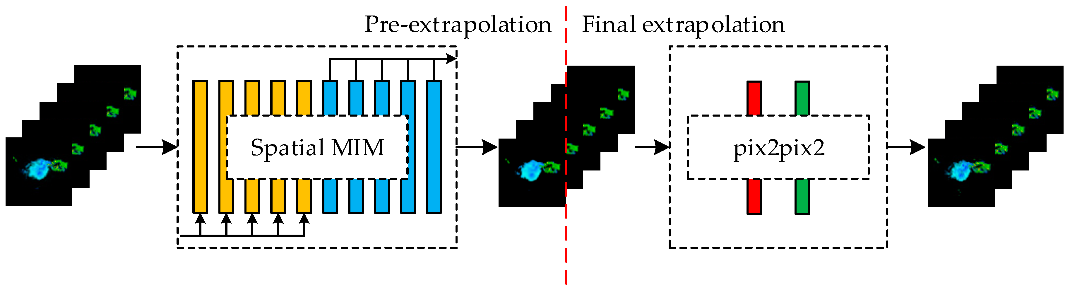
In this paper, we propose a two-stage radar reflectivity images prediction model as shown in Figure 1. In the first stage, the Spatial MIM network is used to make rough predictions of the region and shape of the reflectivity images. The experimental results show that the Spatial MIM network has better prediction performance compared to other methods. This can also show that spatial MIM networks can better retain the spatiotemporal information of the sequence. In the second stage, the Pix2Pix network [37] is used as the optimization model. The reflectivity intensity and internal structure of the predicted image are fine-tuned by optimizing the model. The forecast images are processed through the Pix2Pix network to resolve high reflectivity deficits and local texture deficits due to image blurring. The main contributions of this paper are summarized as follows:
- The traditional method can only predict the changes in the position and shape of cloud clusters. The method in this paper not only predicts the change of reflectivity intensity of cloud clusters but also solves the difficult situation of cloud reflectivity intensity prediction;
- The use of RNN causes the image blurring problem caused by using the MSE loss function. The method in this paper can solve the image blurring problem and better predict the high-frequency component of nonlinearity in reflectivity images;
- The method in this paper can give the prediction results of reflectivity images for five moments and all of them have high reliability.
This paper is organized as follows: Section 1 is an introduction. Section 2 presents the related work. Section 3 describes the dataset and the computer hardware. Section 4 presents the structure of the Spatial MIM network and its experimental results. Section 5 presents the Pix2Pix network and its effects. Section 6 presents the discussions. Section 7 presents the conclusions.
3. Training Preparation
3.1. Data
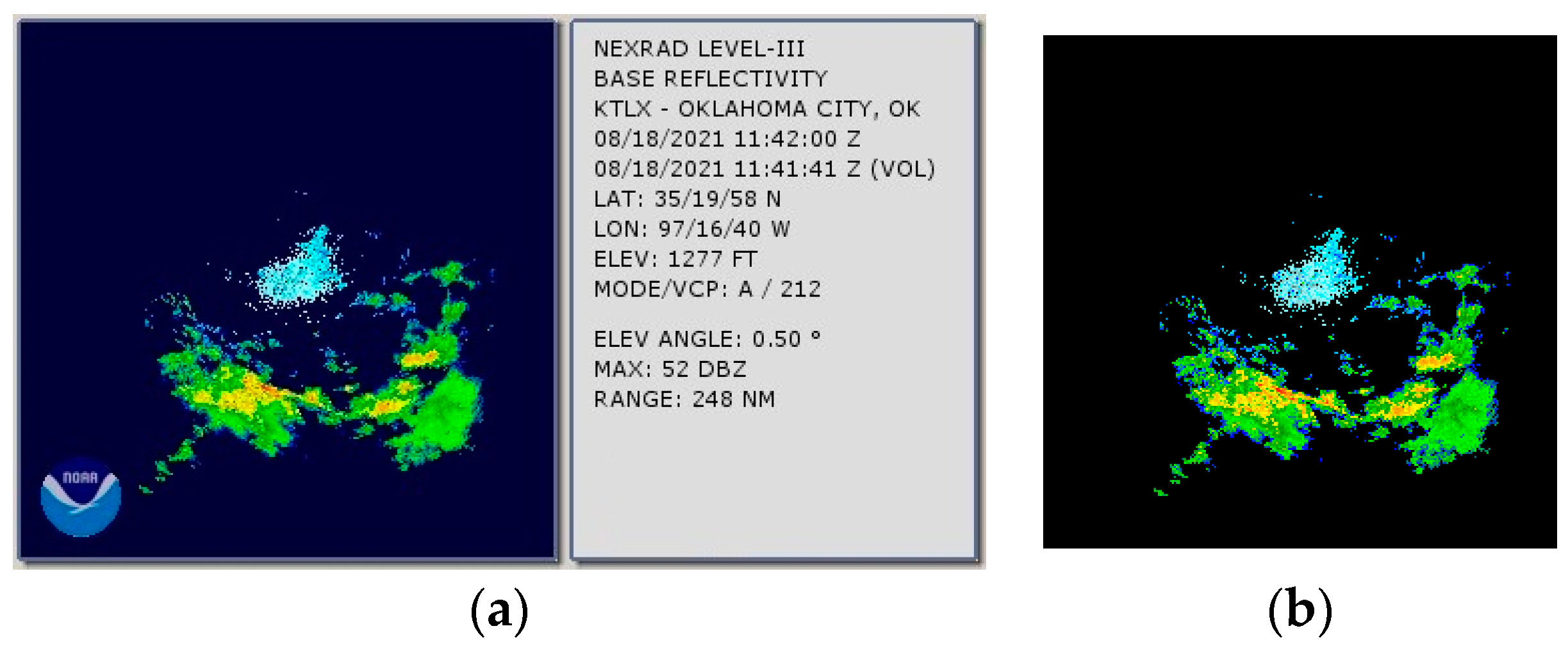
The radar reflectivity images are generated using dual-polarization weather radar data provided by the National Oceanic and Atmospheric Administration (NOAA) of the United States. The reflectivity image is shown in Figure 2a. The radar is located in Oklahoma, Oklahoma, USA, with a latitude of 35.19°N and a longitude of 97.16°W. The radar scan range is 230 km. Each scan includes six elevation angles, ranging from 0.5° to 3.4°. Every 10 consecutive radar scans are considered as a complete set of samples. The first 5 moments of radar reflectivity images are used as inputs to the model to predict the next 5 moments of radar reflectivity images. The latter 5 moments of radar reflectivity images are used as labels to evaluate the model performance. The samples are divided into training and test sets according to the sample recording time under the premise of random division. To ensure the independence between the datasets, under the above constraints, we use a total of 6137 sets of series from April 2021 to September 2021 as the dataset. Among them, the training set sample sequences are 5337 and the test set sample sequences are 800.
3.2. Image Preprocessing
Before starting the training, we need to crop the unnecessary information on the image and only retain the reflectivity image area. Inputting too large reflectivity images will take up a lot of GPU memory resources, while too small images will lose image detail information. With the Java support provided by NOAA, we changed the image size and tested it. Finally, the image size of 256 × 256 is chosen. This scheme can retain as much original image information as possible while reducing the training cost. On this basis, we remove the NOAA logo from the lower left corner of the reflectance image. To enhance the contrast between the foreground and background of the image, the background color is changed to black. The pre-processed image is shown in Figure 2b.
3.3. Experimental Equipment
The model was trained with an Intel i7-10700KF CPU, RTX 3090 GPU and 16 GB RAM. The running environment was Windows 10, Python 3.8.11, tensorflow2.7.0 (A symbolic mathematics system based on data flow programming), CUDA 11.1 (A computing platform launched by NVIDIA), cudnn 8.1.0 (A GPU acceleration library for deep neural networks) and pytorch 1.10.1 (An open-source neural network library).
4. Pre-Extrapolation Model
4.1. The Spatial MIM Network
Time series prediction involves fitting a function to historical moment data to predict future values [38]. An effective prediction model should be able to capture the intrinsic variation in continuous time, which comprises a low-frequency stationarity component and a high-frequency non-stationarity component. While existing methods can fit the low-frequency stationarity component well, accurately modeling the high-frequency non-stationarity component remains a significant challenge in time series prediction tasks. In particular, the radar reflectivity image sequence is a natural space-time process in which adjacent pixels are closely related, and their joint distribution rapidly changes with time, resulting in complex non-stationarity in both time and space. Therefore, learning the high-frequency components based on temporal and spatial non-stationarity is crucial for radar reflectivity image prediction tasks.
The results of the study reveal [31] that while models such as PredRNN have made some progress in addressing the issue of temporal and spatial information transfer, their forgetting gate settings are overly simplistic and cannot effectively predict higher-order components of spatiotemporal non-stationarity. This drawback leads to partial blurring of the predicted image and diminishes the model’s prediction effectiveness. Specifically, experiments [29] using the PredRNN model for precipitation prediction reveal that the forgetting gate is saturated in 80% of the time, leading to a significant loss of high-frequency non-stationarity components in the forecast process. Consequently, the prediction results are dominated by the forecasts of low-frequency stationarity components.
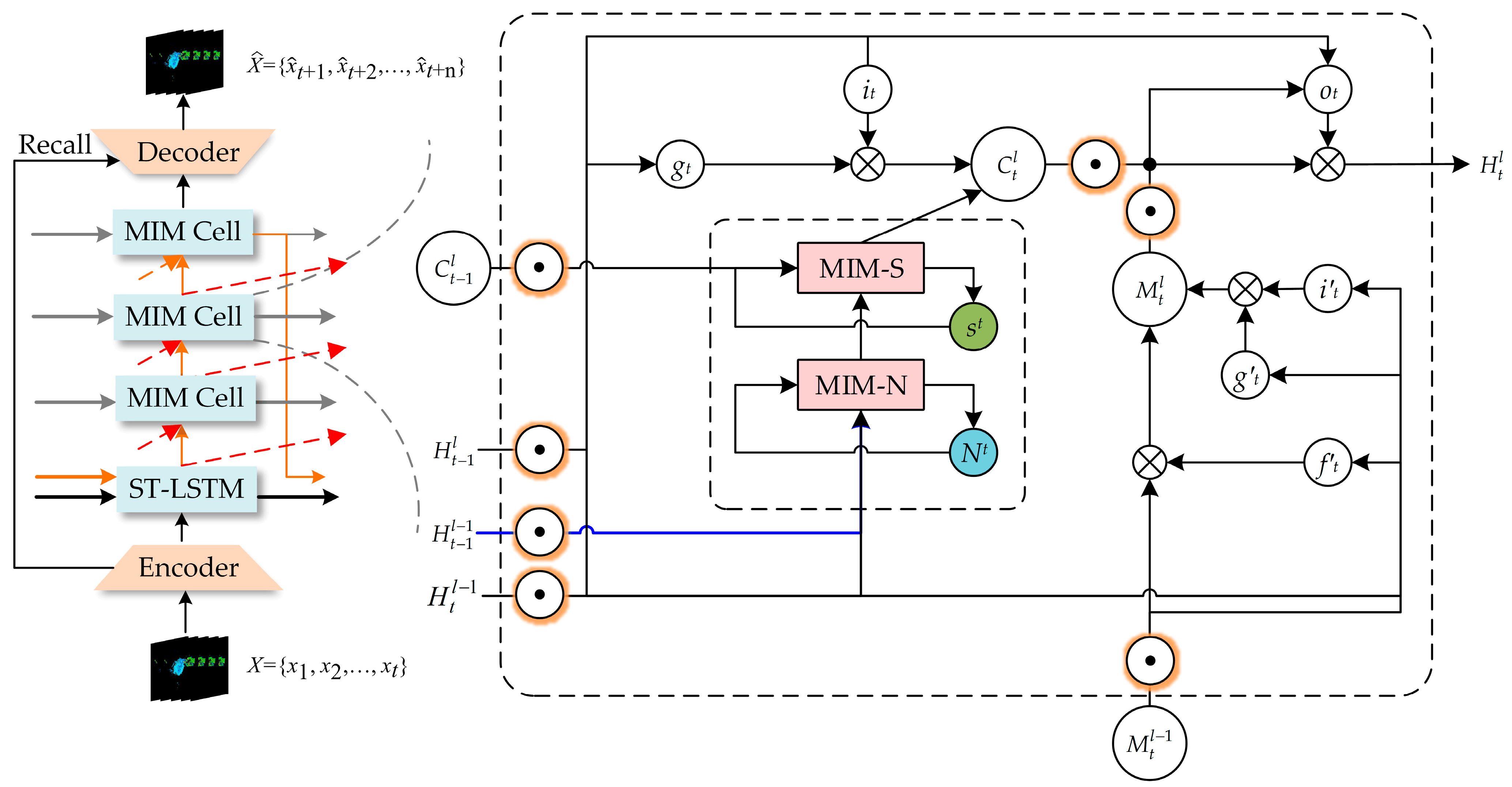
In comparison to the PredRNN, the proposed model provides better prediction of the higher-order components of spatiotemporal non-stationarity. Specifically, the input images to the Spatial MIM network are radar reflectivity images with a sequence length of five, and the output is a sequence of radar reflectivity images at future 5 moments. The Spatial MIM network is a six-layer network comprising an encoder, an ST-LSTM layer, three modified MIM layers and a decoder layer. The design of the Spatial MIM network is derived from the MIM network, which aims to replace the easily saturated forgetting gate in the ST-LSTM network with two cascaded temporal memory modules.
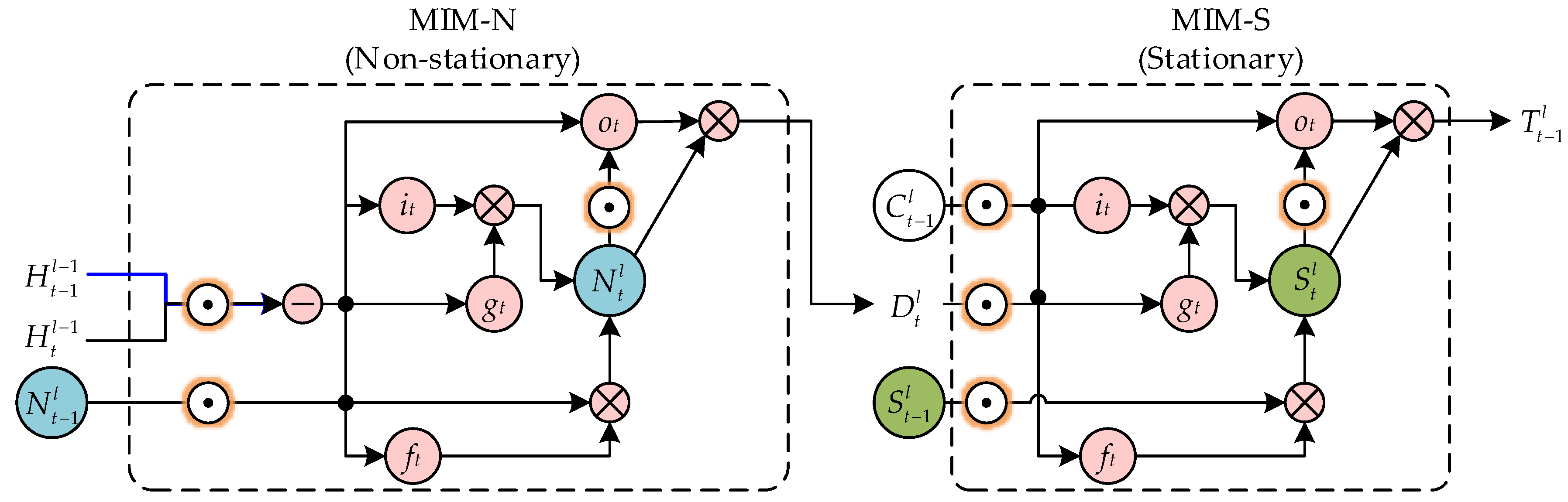
The memory module is shown in Figure 3 and Figure 4. Its formulas can be expressed as follows:
where Ntl and Stl denote the memory units in MIM-N and MIM-S, respectively, Dtl is learned by MIM-N and used as the input of MIM-S, Ttl is the memory passing the virtual “forget gate”, Ctl is the standard temporal cell, Mtl is the spatiotemporal memory, Htl is the hidden state, it is the input gate, ot is the output gate, ft is the forget gate, gt is the input-modulation gate, σ is sigmoid activation function and * means that function A acts on array B in A * B.
The first module is a non-stationarity module with inputs htl−1 and ht-1l−1. This module represents high-frequency non-stationary changes through the difference between the two inputs. The second module is the stationary module, and the input is the output of the non-stationary module Dtl and the external temporary memory Ct-1l. This module is used to represent low-frequency stationarity variations in spatiotemporal sequences. The above two modules are cascaded and used to replace the forgetting gate in ST-LSTM. It can better forecast high-frequency non-stationary variations. The formulas for the MIM-N module are shown as follows:
where the non-stationary variation in the spatiotemporal series is represented by the difference (Htl−1 − Ht−1l−1). The formulas of the MIM-S module are shown as follows:
When the value of differential feature Dtl is very small, the non-stationary variation is not severely expressed. At this time, the MIM-S module will mainly use the original memory. When the value of the difference feature Dtl is large, the MIM-S module will overwrite the original memory.
During training, the encoder and decoder [39,40] are required to effectively transfer information from the bottom layer to the top layer and preserve the spatial high-frequency components of the image. The encoder encodes the input Xt into deep features, which extract useful spatial information that helps the state transfer unit make accurate spatial predictions. The decoder saves the useful spatial information and decodes the predicted spatial states as outputs.
The structure diagram of the Spatial MIM network is shown in Figure 4, and the formulas of the encoder and decoder are presented as follows:
where Enc denotes encoder and Dec denotes decoder.
Considering that some high-frequency components of spatial information will be lost during encoding, the information recall scheme is used when constructing the encoder and decoder. By using the information recall scheme, each layer of the decoder can obtain information from multiple layers of the encoder. This information can help generate better forecast images with a more complete retention of the high-frequency component of spatial information. The formula of the information recall scheme is shown as follows:
where Dl denotes the decoding features from layer l of the decoder and El~N denotes the encoding features from layer l to layer N of the encoder.
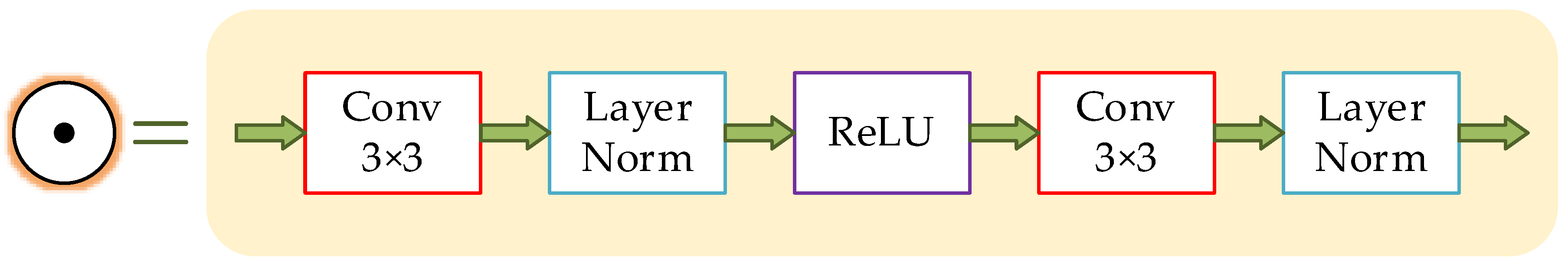
In this paper, we replace the 5 × 5 convolution filter in the MIM module with two 3 × 3 convolution filters and change the normalization method, resulting in three advantages: increased network depth, reduced model parameters and reduced risk of the exploding gradient problem. The orange circles in Figure 3 and Figure 4 represent our modified two-layer convolutional filter, which consists of a convolutional layer, a LayerNorm layer and a ReLU layer. The structure is shown in Figure 5. The first convolutional layer of the two-layer convolutional filter is followed by a ReLU activation function, and the second convolutional layer is followed by a tanh or sigmoid activation function.
4.2. Prediction Results of the Spatial MIM Network
In this section, we present the experimental results of the proposed Spatial MIM network and compare it with other models, namely Convlstm, PredRNN, PredRNN++ and MIM. To evaluate the performance of the models, we use evaluation indicators and analyze the results. All models were trained using 5337 sample sequences and tested using 800 sample sequences to evaluate the model performance.
The original radar reflectivity image is a 220-graded pseudo-color image, and the radar reflectivity image obtained from the forecast is a color image. Therefore, we perform a similarity measure for each pixel point in the forecast radar reflectivity image and convert the image to a 220-graded pseudo-color image.
4.2.1. Meteorological Evaluation Indicators
To evaluate the models under different degrees of meteorological disasters, a threshold is set for the reflectivity intensity. Pixel points with reflectivity intensity lower than the reflectivity threshold are changed to background black, while pixel points with reflectivity intensity larger than the reflectivity threshold retain their original color. The evaluation is conducted by classifying each point on the forecast image after setting the threshold as “predicted yes” or “predicted no”. Likewise, each point on the labeled image after setting the threshold is classified as “observed yes” or “observed no”. The details are shown in Table 1.
POD, FAR, CSI and ETS, which are commonly used in the field of meteorology, were selected as evaluation indicators, and the formulas are shown below.
The POD represents the proportion of successful forecasts among the total number of events; the FAR represents the proportion of incorrect forecasts among the total number of forecast events; the CSI represents the comprehensive level of POD and FAR; the ETS represents a more comprehensive evaluation of hits through penalizing misses and false alarms and adjusting hits associated with random chance. Larger POD, CSI and ETS values indicate greater model performance, while smaller FAR values indicate greater model performance.
Using the POD, FAR, CSI and ETS scores evaluated from the test set, we quantitatively assess the model’s overall performance. Table 2 lists the POD, FAR, CSI and ETS scores of the models with the threshold of 0 DBZ. Compared with the Convlstm, the other four models have higher POD, CSI and ETS scores. Although the Convlstm outperforms the other four models in FAR during the first two prediction moments, it falls short in subsequent moments. The PredRNN outperforms the Convlstm on POD, CSI and ETS scores but falls short on FAR score, showing that its predicted results are more accurate and closer to reality. At the same time, the experiments result also exhibits the ST-SLTM module’s effectiveness. When compared to the PredRNN, the PredRNN++ and the MIM perform better. As a result, the feasibility of using cascaded memory modules to replace ST-SLTM modules was demonstrated. Among the five models, the Spatial MIM model proposed in this article has the highest POD, CSI and ETS scores while also having the least FAR score. The Spatial MIM achieved the best prediction results, proving the superiority of the proposed method.
Table 3, Table 4 and Table 5 list the POD, FAR, CSI and ETS scores of the models with the threshold of 20, 25 and 30 DBZ. When the threshold value is 30DBZ, the MIM has a lower FAR score than the Spatial MIM and a lower fraction of prediction error events. However, it is clear that the Spatial MIM proposed in this paper has higher POD, CSI and ETS scores while having a lower FAR score most of the time. Experiments show that the Spatial MIM proposed in this paper can complete the spatiotemporal modeling well and forecast convective weather more accurately.
4.2.2. Mathematical Evaluation Indicators
The most common mathematical evaluation indicators used for assessing the performance of prediction models are Mean Absolute Error (MAE), Root-Mean-Square Error (RMSE), Correlation Coefficient (CC), Skill Score (SS), Mean Error (ME) and Normalized Root-Mean-Square Error (NRMSE). Thus, the mathematical evaluation indicators used in this paper are expressed as follows:
where and represents the actual pixel values and the predicted pixel values, n represents the total number of pixels, MSES represents the MSE score of the Spatial MIM and MSEf represents the MSE score of the comparison network.
Larger CC, SS values indicate greater model performance, while smaller MAE, RMSE, NRMSE values indicate greater model performance. At the same time, ME value closer to 0 indicate greater model performance.
The mathematical evaluation indicators of the models averaged over all moments and the time required to predict a time series are listed in Table 6. In comparison to Convlstm and PredRNN, the other three models have higher CC value and lower SS value. This represents an improvement in the correlation between the forecast and real images, as well as a decrease in forecast error. Although the RMSE value for RredRNN++ and MAE and ME values for MIM are the same as for the Spatial MIM, the Spatial MIM performs better on other Mathematical evaluation indicators. Although the increased network depth adds some time consumption. In a sequence of radar reflectivity images, the time interval between two neighboring images is severe minutes, whereas our prediction of a complete sequence takes 0.97 s. This time consumption is acceptable in comparison to the performance improvement. In summary, the prediction method presented in this paper can perform better in the area of radar reflectivity image prediction.
4.2.3. Ablation Study
We performed an ablation study on the spatial MIM network to validate the effectiveness of the model improvement. The details are shown in Table 7 and Table 8:
The evaluation indicators reveals that the performance of the Spatial MIM is not only superior to MIM, but also better than the Spatial MIM with no E and the Spatial MIM with no D. It can be seen that the improvements made in this paper for the MIM are effective and can better predict the radar reflectivity images.
4.2.4. Reflectivity Forecast Images
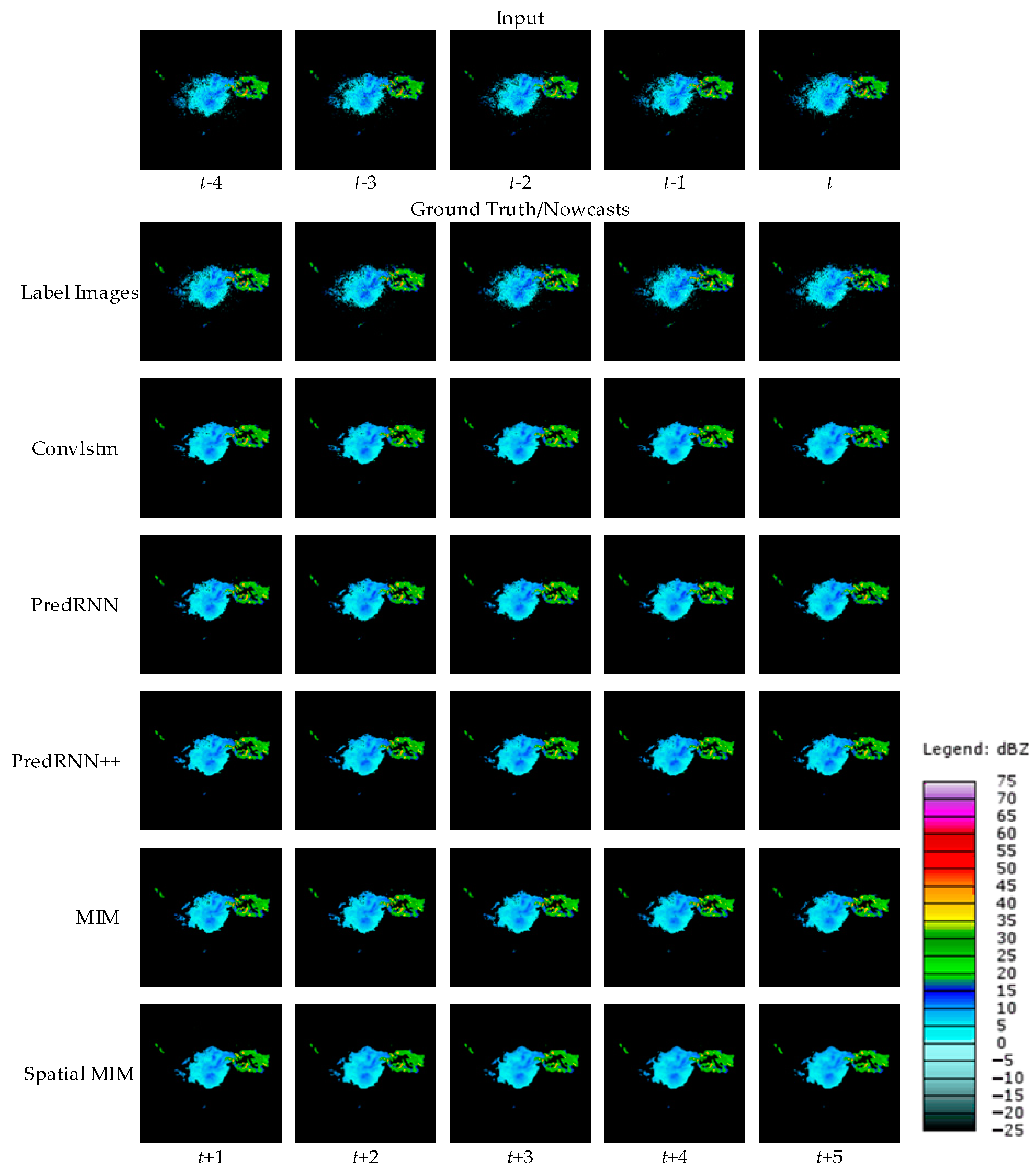
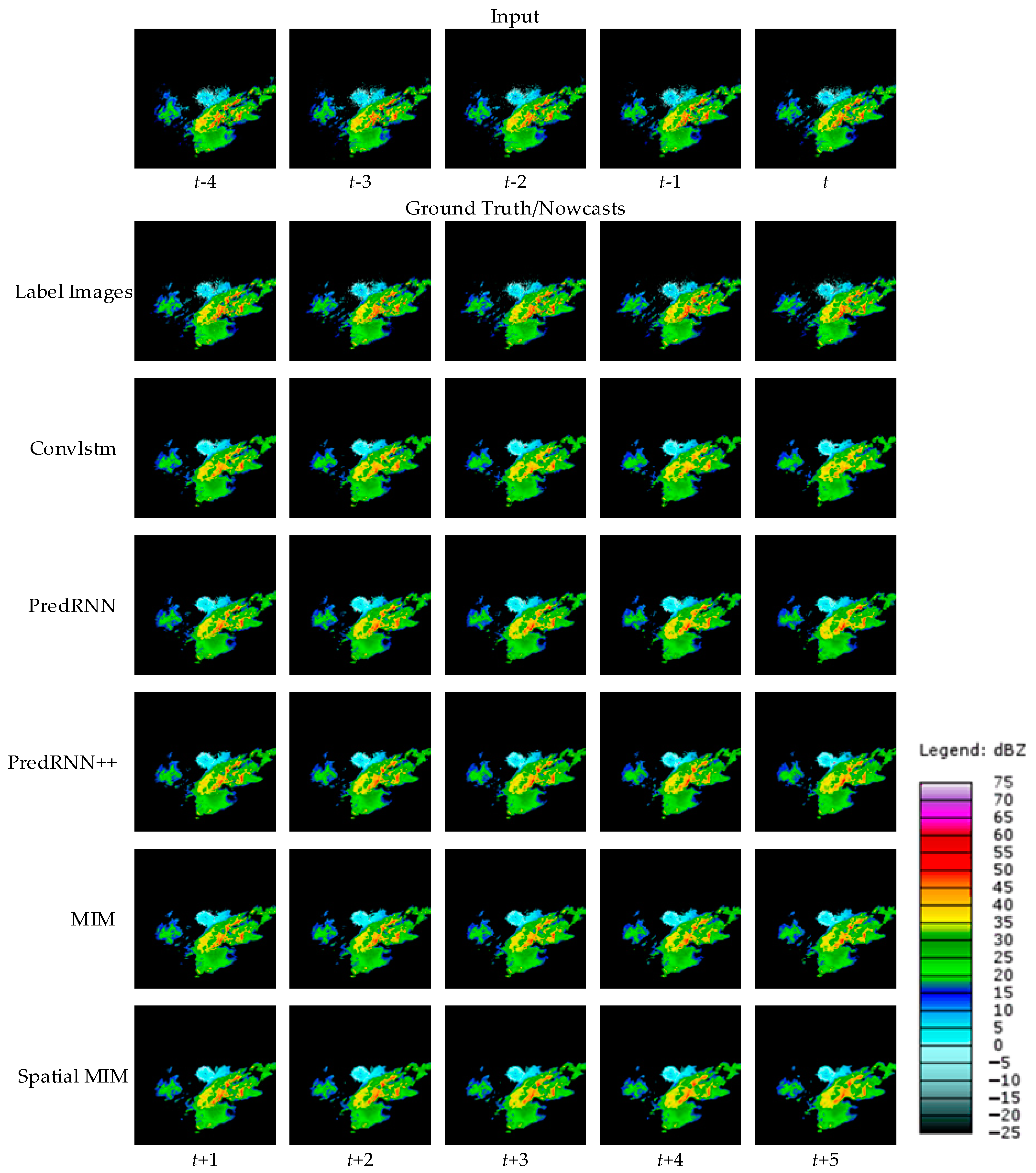
To visually represent the performance of the model proposed in this paper, two cases are randomly selected from the test set and the forecast results of different models are shown. Figure 6 and Figure 7 show the observed images and forecast results of the two cases.
As demonstrated by the above two cases, all four comparison models can produce roughly accurate prediction predictions. However, compared with other comparable models, Spatial MIM produces better extrapolation results. At the same time, it can complete as much of the forecast of high-frequency components as possible while minimizing detail loss. Through the evaluation indexes and forecast images, it is easy to see that Spatial MIM has superior spatial and temporal modeling capabilities for the complex nonlinear process of convective echoes. While RNN networks provide accurate forecasts, they do have limits, which are described in detail in Section 4.
5. Post-Processing Model
This section discusses the limitations of radar reflectivity images in capturing three-dimensional information, as well as the blurring effect that occurs when predicting with RNN models. The use of MSE loss functions in RNN models can result in image smoothing and reduced high-frequency component forecast accuracy. While the Spatial MIM model presented in the previous section demonstrated accurate low-frequency component prediction, its high-frequency component prediction accuracy is still lacking in two areas: high reflectivity deficits and local texture deficits due to image blurring. Accurate high-frequency component prediction is critical in convective weather prediction, so this section focuses on it. To address this, the Pix2Pix network-based post-processing model is proposed to improve the accuracy of high-frequency component forecasts.
5.1. Pix2Pix Method
GAN is a traditional neural network with a generator and discriminator model. The generator model is used to generate images in the field of image processing. The generator receives a random noise z and calculates the noise z to generate a false image G(z). The discriminator determines whether the generated image is true or false. The discriminator’s inputs are G(z) and the label image, and the output D(G(z)) represents whether G(z) is a real image. During training, the generator’s goal is to generate fake images in order to deceive the discriminator, rendering the discriminator unable to distinguish the generated images from the real ones.
The generator and discriminator are trained together, and the training process is turned into a game. Simultaneously, the generator and discriminator gradually improve their capabilities until they reach a Nash equilibrium. GAN overcomes the limitations imposed by traditional image generation models due to the use of loss functions. The discriminator works similarly to a loss function, allowing the model to be improved continuously. The loss function of the GAN network is shown below:
where G denotes the generator, D denotes the discriminator, E denotes the mathematical expectation, y denotes the real image and z denotes the noise used to generate the image.
Traditional GAN networks take noise z as input and investigate the mapping of noise z to image y. There is no obvious relationship between the generator’s input and output, making it challenging to deal with complex applications. In contrast to GAN networks, CGAN networks [41] use the condition x and noise z as the generator’s input. The generator and the discriminator are continuously confronted to complete the network training. The loss function of the CGAN network is shown as follows:
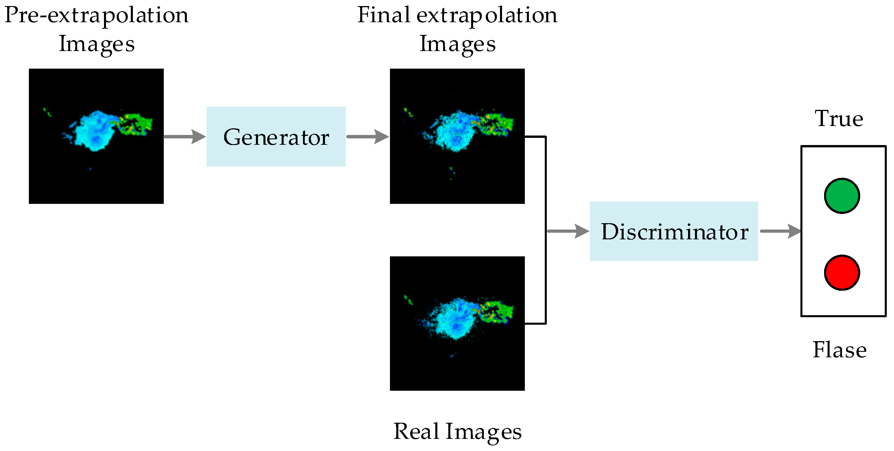
The Pix2Pix network is a type of architecture for conditional generative adversarial networks (cGAN). In this paper, we use the Pix2Pix network to improve the Spatial MIM network’s forecast results and solve the problem of blurred forecast images. The forecasts from the Spatial MIM network are fed into the generator and the improved forecasts are output. The discriminator receives both the improved and real images as input and outputs either 0 or 1. The output is 1 when the discriminator considers the improved image to be a positive sample. The output is 0 when the discriminator considers the improved image to be a negative sample. The structure diagram of the Pix2pix network is shown in Figure 8.
5.2. Model Structure
5.2.1. Generator
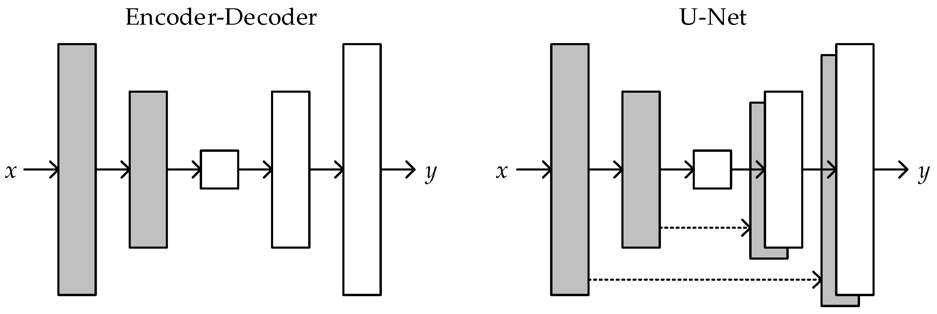
Image translation is the process of converting a high-resolution image to another high-resolution image. Although the images’ content differs before and after translation, they all have the same underlying structure. As a result, an encoder–decoder network is commonly used as a generator in practice. The network meets the basic criterion of having roughly symmetrical input and output structures. The input enters the generator and passes through a compression path and an expansion path. The data is down-sampled by several convolution–BatchNorm–ReLu modules in the compression path before entering the expansion path after reaching the bottleneck layer. Deconvolution is used to perform up-sampling in the expansion path. The image information goes across all layers of the generator network when the encoder–decoder is used as a generator, resulting in partial information loss.
To ensure that low-level information is well transferred between input and output and that the generated image can recover high-frequency components more effectively. Add skip connections between the compressed and expanded paths using the U-Net form. Skip connections are added between layer i and layers n-i, where n is the total number of layers. Each skip connection’s function is to connect all channels at layer i to layer n-i. The structure diagram is shown in Figure 9.
5.2.2. Markovian Discriminator (PatchGAN)
The Markovian discriminator (PatchGAN) is used as a discriminator to better recover the high-frequency components of the forecast image and to reduce the discriminator’s computational complexity. The original GAN’s discriminator only produces a single evaluation value, which is used to determine whether the image is true or false. The input image will not directly enter the full connection layer after passing through the convolution layer but will be mapped into an N × N matrix through convolution. Each matrix point represents the evaluation value of a small portion of the original image. Evaluating the entire image with one value is converted to evaluating the whole image through an N × N matrix. The final output of the discriminator is determined by averaging all the evaluation values. The use of PatchGAN reduces the computational effort and allows for better recovery of the high-frequency components of the local image.
5.2.3. Loss Function
In traditional GAN, the L2 loss and the GAN objective are commonly mixed as the network’s loss function. The L1 loss is used instead of the L2 loss to provide a better solution to the image blurring caused by using RNN and to better recover the high-frequency components of the forecast images. The L1 loss is calculated as:
Our final loss function is:
where LcGAN denotes the GAN objective and λ denotes a constant coefficient.
Increasing the noise z at input had an insignificant effect on preventing the generation of fixed results. Most of the time the generator learns to ignore the noise through training. In this paper, we replace the input noise z with noise in the form of dropout, which is applied to several layers of our generator during both training and testing.
5.3. Results of the Pix2Pix Network
The inputs of the Pix2Pix network are the outputs of the Spatial MIM, with the high-frequency components missing in part. The Pix2Pix network was trained and tested using the same sample sequences as the Spatial MIM, with 5337 sample sequences were used for training and 800 sample sequences were used for testing to evaluate model performance.
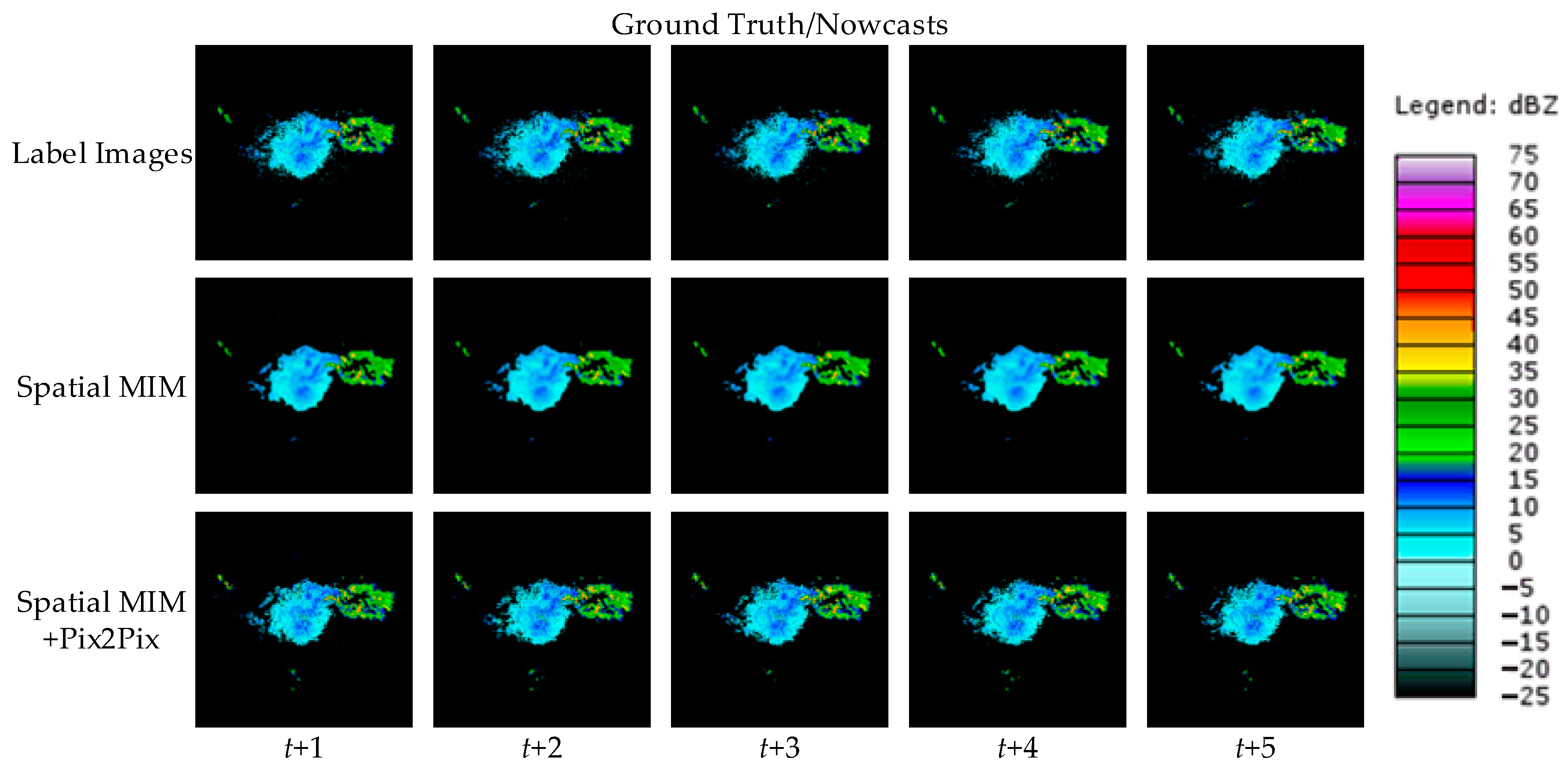
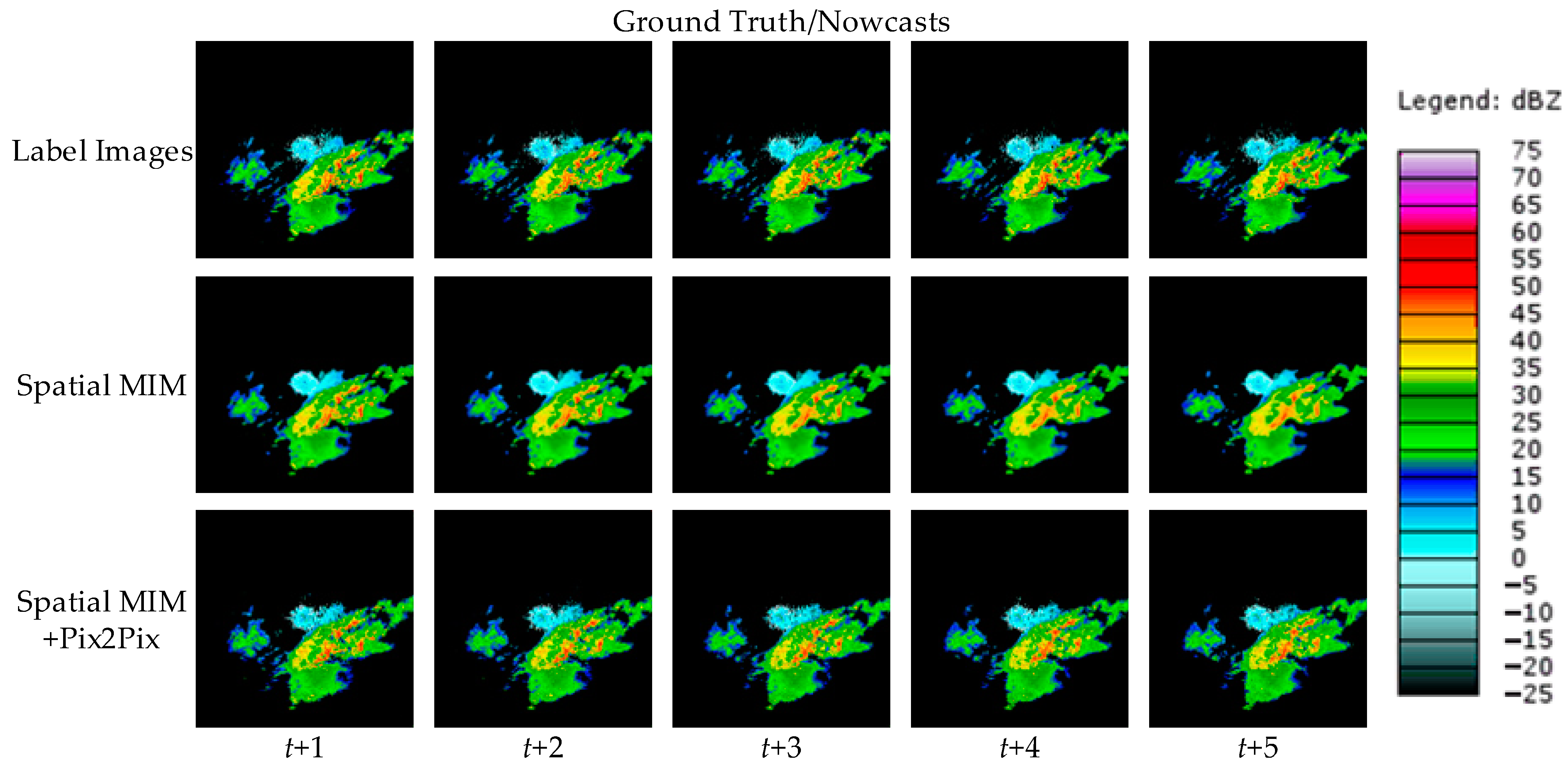
To visualize the model’s performance after adding the Pix2Pix network, we show the prediction results before and after adding the Pix2Pix network for the two cases as shown in Figure 10 and Figure 11.
As shown in Figure 10 and Figure 11, the addition of the Pix2Pix network restores some of the detail information of the forecast image. This is manifested in two ways: the reduction of high reflectivity deficits and the reduction of local texture deficits due to image blurring. This demonstrates that the prediction accuracy of the high-frequency component of the forecast image has improved. The method used in this paper allows future studies such as precipitation prediction and it is effective and can be encouraged for application.
6. Discussion
Although the method in this paper performs well, there are several limitations that need be addressed in the future. First, radar reflectivity images are time sensitive. When the original images surpass the radar echo lifetime, predicting the formation and demise of a cloud mass becomes challenging. Second, after several moments of development, similar radar reflectivity images may yield different live weather. As a result, uncertainty in prediction findings may exist during real prediction, which is one of the challenges of reflectivity image prediction. Third, the speed of cloud mass migration influences accuracy. When the motion speed of the cloud mass is too quick, the forecast’s accuracy may suffer. In summary, for most types of radar reflectivity echoes, our method can effectively conduct motion trajectory prediction, reflectivity intensity prediction and echo shape prediction.
7. Conclusions
We propose a deep learning-based reflectivity image prediction algorithm in this paper. We offer a method that combines pre-extrapolation and final extrapolation to address the problems of blurring and loss of high-frequency components in forecast images produced by MSE functions. We optimize the model structure and add codecs during the pre-extrapolation stage. And at the final extrapolation stage, we use the Pix2Pix network to improve the forecast image blurring problem.
In comparison to the traditional method, the method presented in this paper can achieve continuous prediction of reflectivity images. The forecast results have better small-scale details and are more consistent with the real radar reflectivity images. Our method is more accurate in predicting cloud masses that may cause severe weather.
Despite the fact that we employ the Pix2Pix network to reduce image blurring produced by the MSE loss function and to collect high-frequency information, there is still a gap between the prediction images and the actual images. Further in-depth research is still required to improve the forecast image quality. Simultaneously, the employment of GAN raises certain concerns, such as whether it will have a negative impact on later precipitation prediction efforts.
To summarize, precisely predicting the motion of clouds in the sky from reflectivity images alone remains a difficult task. Wind field data, environmental field data and spectral data must all be examined in order to achieve more precise forecast results. In future studies, we will build models that are jointly driven by environmental field data and radar reflectivity data to improve prediction results.
Author Contributions
Conceptualization, Z.L. and J.G.; methodology, J.G.; software, J.G.; validation, Z.L. and J.G.; formal analysis, J.G.; investigation, Q.Y.; resources, Z.L.; data curation, J.G.; writing—original draft preparation, J.G.; writing—review and editing, Z.L. and J.Z.; project administration, J.Z.; funding acquisition, Z.L. All authors have read and agreed to the published version of the manuscript.
Funding
This research received no external funding.
Data Availability Statement
For this study, we used an open-source and governmental dataset from the address: National Oceanic and Atmospheric Administration (NOAA) National Climatic Data Center. The data is available at https://www.ncdc.noaa.gov/nexradinv/ (accessed on 11 April 2022).
Conflicts of Interest
The authors declare no conflict of interest.
References
- Geng, F.; Liu, L. Study on Attenuation Correction for the Reflectivity of X-Band Dual-Polarization Phased-Array Weather Radar Based on a Network with S-Band Weather Radar. Remote Sens. 2023, 15, 1333. [Google Scholar] [CrossRef]
- Garcia-Benadi, A.; Bech, J.; Udina, M.; Campistron, B.; Paci, A. Multiple Characteristics of Precipitation Inferred from Wind Profiler Radar Doppler Spectra. Remote Sens. 2022, 14, 5023. [Google Scholar] [CrossRef]
- Wang, P.; Shi, J.; Hou, J. The Identification of Hail Storms in the Early Stage Using Time Series Analysis. J. Geophys. Res. 2018, 123, 929–947. [Google Scholar] [CrossRef]
- Shi, J.; Wang, P.; Wang, D.; Jia, H. Radar-Based Automatic Identification and Quantification of Weak Echo Regions for Hail Nowcasting. Atmosphere 2019, 10, 325. [Google Scholar] [CrossRef]
- Sun, Y.; Zhou, Z.; Gao, Q.; Li, H.; Wang, M. Evaluating Simulated Microphysics of Stratiform and Convective Precipitation in a Squall Line Event Using Polarimetric Radar Observations. Remote Sens. 2023, 15, 1507. [Google Scholar] [CrossRef]
- Pulkkinen, S.; Chandrasekar, V.; Lerber, A.V. Nowcasting of Convective Rainfall Using Volumetric Radar Observations. IEEE Trans. Geosci. Remote Sens. 2020, 58, 7845–7859. [Google Scholar] [CrossRef]
- Pulkkinen, S.; Chandrasekar, V.; Harri, A.M. Fully Spectral Method for Radar-Based Precipitation Nowcasting. IEEE J. Sel. Topics Appl. Earth Observ. Remote Sens. 2019, 12, 1369–1382. [Google Scholar] [CrossRef]
- Cao, Y.; Zhang, D.; Zheng, X.; Shan, H.; Zhang, J. Mutual Information Boosted Precipitation Nowcasting from Radar Images. Remote Sens. 2023, 15, 1639. [Google Scholar] [CrossRef]
- Guo, S.; Sun, N.; Pei, Y.; Li, Q. 3D-UNet-LSTM: A Deep Learning-Based Radar Echo Extrapolation Model for Convective Nowcasting. Remote Sens. 2023, 15, 1529. [Google Scholar] [CrossRef]
- Pop, L.; Sokol, Z.; Minarova, J. Nowcasting of the probability of accumulated precipitation based on the radar echo extrapolation. Atmos. Res. 2018, 216, 1–10. [Google Scholar] [CrossRef]
- Rinehart, R.E.; Garvey, E.T. Three-dimensional storm motion detection by conventional weather radar. Nature 1978, 273, 287–289. [Google Scholar] [CrossRef]
- Zou, H.; Wu, S.; Shan, J. A Method of Radar Echo Extrapolation Based on TREC and Barnes Filter. J. Atmos. Ocean. Technol. 2019, 36, 1713–1727. [Google Scholar] [CrossRef]
- Zahraei, A.; Hsu, K.L.; Sorooshian, S. Quantitative Precipitation Nowcasting: A Lagrangian Pixel-Based Approach. Atmos. Res. 2012, 118, 418–434. [Google Scholar] [CrossRef]
- Liu, Y.; Xi, D.G.; Li, Z.L. A new methodology for pixel-quantitative precipitation nowcasting using a pyramid Lucas Kanade optical flow approach. J. Hydrol. 2015, 529, 354–364. [Google Scholar] [CrossRef]
- Dixon, M.; Wiener, G. TITAN: Thunderstorm Identification, Tracking, Analysis, and Nowcasting—A Radar-based Methodology. J. Atmos. Ocean. Technol. 1993, 10, 785–797. [Google Scholar] [CrossRef]
- Johnson, J.T.; MacKeen, P.L.; Witt, A.; Mitchell, E.D.W.; Stumpf, G.J.; Eilts, M.D.; Thomas, K.W. The Storm Cell Identification and Tracking Algorithm: An Enhanced WSR-88D Algorithm. Weather Forecast. 1998, 13, 263–276. [Google Scholar] [CrossRef]
- Walker, J.R.; MacKenzie, W.M.; Mecikalski, J.R.; Jewett, C.P. An Enhanced Geostationary Satellite–Based Convective Initiation Algorithm for 0–2-h Nowcasting with Object Tracking. J. Appl. Meteorol. Climatol. 2012, 51, 1931–1949. [Google Scholar] [CrossRef]
- Rossi, P.J.; Chandrasekar, V.; Hasu, V.; Moisseev, D. Kalman filtering based probabilistic nowcasting of object-oriented tracked convective storms. J. Atmos. Ocean. Technol. 2015, 32, 461–477. [Google Scholar] [CrossRef]
- Muñoz, C.; Wang, L.P.; Willems, P. Enhanced object-based tracking algorithm for convective rain storms and cells. Atmos. Res. 2018, 201, 144–158. [Google Scholar] [CrossRef]
- Ayzel, G.; Heistermann, M.; Winterrath, T. Optical flow models as an open benchmark for radar-based precipitation nowcasting (rainymotion v0.1). Geosci. Model Dev. 2019, 12, 1387–1402. [Google Scholar] [CrossRef]
- Woo, W.-c.; Wong, W.-k. Operational Application of Optical Flow Techniques to Radar-Based Rainfall Nowcasting. Atmosphere 2017, 8, 48. [Google Scholar] [CrossRef]
- Bowler, N.E.; Pierce, C.E.; Seed, A. Development of a precipitation nowcasting algorithm based upon optical flow techniques. J. Hydrol. 2004, 288, 74–91. [Google Scholar] [CrossRef]
- Lagerquist, R.; McGovern, A.; Smith, T. Machine learning for real-time prediction of damaging straight-line convective wind. Weather Forecast. 2017, 32, 2175–2193. [Google Scholar] [CrossRef]
- Jergensen, G.E.; McGovern, A.; Lagerquist, R.; Smith, T. Classifying convective storms using machine learning. Weather Forecast. 2020, 1, 537–559. [Google Scholar] [CrossRef]
- Asanjan, A.A.; Yang, T.; Hsu, K.; Sorooshian, S.; Lin, J.; Peng, Q. Short-term precipitation forecast based on the Persiann system and LSTM recurrent neural networks. J. Geophys. Res. Atmos. 2018, 123, 12543–12563. [Google Scholar]
- Lu, Z.; Wang, Z.; Li, X.; Zhang, J. A Method of Ground-Based Cloud Motion Predict: CCLSTM + SR-Net. Remote Sens. 2021, 13, 3876. [Google Scholar] [CrossRef]
- Shi, X.; Chen, Z.; Wang, H.; Yeung, D.; Wong, W.; Woo, W. Convolutional LSTM Network: A Machine Learning Approach for Precipitation Nowcasting. In Proceedings of the 29th Annual Conference on Neural Information Processing Systems, Montreal, QC, Canada, 7–12 December 2015; Volume 28. [Google Scholar]
- Shi, X.; Gao, Z.; Lausen, L.; Wang, H.; Yeung, D.-Y.; Wong, W.-K.; Woo, W.-C. Deep learning for precipitation nowcasting: A benchmark and a new model. In Proceedings of the Advances in Neural Information Processing Systems, Long Beach, CA, USA, 4–9 December 2017; pp. 5618–5628. [Google Scholar]
- Wang, Y.; Long, M.; Wang, J.; Gao, Z.; Yu, P.S. PredRNN: Recurrent Neural Networks for Predictive Learning using Spatiotemporal LSTMs. In Proceedings of the 31st Annual Conference on Neural Information Processing Systems, Long Beach, CA, USA, 4–9 December 2017; Volume 30. [Google Scholar]
- Wang, Y.; Gao, Z.; Long, M.; Wang, J.; Yu, P.S. PredRNN++: Towards A Resolution of the Deep-in-Time Dilemma in Spatiotemporal Predictive Learning. In Proceedings of the 35th International Conference on Machine Learning, Stockholmsmässan, Stockholm, Sweden, 10–15 July 2018; Volume 80, pp. 5123–5132. [Google Scholar]
- Wang, Y.; Zhang, J.; Zhu, H.; Long, M.; Wang, J.; Yu, P.S. Memory in Memory: A Predictive Neural Network for Learning Higher-Order Non-Stationarity From Spatiotemporal Dynamics. In Proceedings of the 2019 IEEE/CVF Conference on Computer Vision and Pattern Recognition (CVPR), Long Beach, CA, USA, 15–20 June 2019; pp. 9146–9154. [Google Scholar]
- Wang, C.; Wang, P.; Wang, P.; Xue, B.; Wang, D. Using Conditional Generative Adversarial 3-D Convolutional Neural Network for Precise Radar Extrapolation. IEEE J. Sel. Top. Appl. Earth Obs. Remote Sens. 2021, 14, 5735–5749. [Google Scholar] [CrossRef]
- Mathieu, M.; Couprie, C.; LeCun, Y. Deep multi-scale video prediction beyond mean square error. In Proceedings of the 4th International Conference on Learning Representations, San Juan, PR, USA, 2–4 May 2016; pp. 1–14. [Google Scholar]
- Goodfellow, L.J.; Pouget-Abadie, J.; Mirza, M.; Xu, B.; Warde-Farley, D.; Ozair, S.; Courville, A.; Bengio, Y. Generative Adversarial Nets. In Proceedings of the 28th Conference and Workshop on Neural Information Processing Systems, Montreal, QC, Canada, 8–13 December 2014; pp. 2672–2680. [Google Scholar]
- Tian, L.; Li, X.; Ye, Y.; Xie, P.; Li, Y. A Generative Adversarial Gated Recurrent Unit Model for Precipitation Nowcasting. IEEE Geosci. Remote Sens. Lett. 2020, 17, 601–605. [Google Scholar] [CrossRef]
- Xie, P.; Li, X.; Ji, X.; Chen, X.; Chen, Y.; Liu, J.; Ye, Y. An Energy-Based Generative Adversarial Forecaster for Radar Echo Map Extrapolation. IEEE Geosci. Remote Sens. Lett. 2022, 19, 3500505. [Google Scholar] [CrossRef]
- Isola, P.; Zhu, J.; Zhou, T.; Efros, A. Image-to-Image Translation with Conditional Adversarial Networks. In Proceedings of the 2017 IEEE Conference on Computer Vision and Pattern Recognition (CVPR), Honolulu, HI, USA, 21–26 July 2017; pp. 5967–5976. [Google Scholar]
- Pan, X.; Lu, Y.; Zhao, K.; Huang, H.; Wang, M.; Chen, H. Improving Nowcasting of Convective Development by Incorporating Polarimetric Radar Variables Into a Deep-Learning Model. Geophys. Res. Lett. 2021, 48, 21. [Google Scholar] [CrossRef]
- Che, H.; Niu, D.; Zang, Z.; Cao, Y.; Chen, X. ED-DRAP: Encoder-Decoder Deep Residual Attention Prediction Network for Radar Echoes. IEEE Geosci. Remote Sens. Lett. 2022, 19, 1004705. [Google Scholar] [CrossRef]
- Cheng, Z.; Zhang, X.; Wang, S.; Ma, S.; Ye, Y.; Xiang, X.; Gao, W. MAU: A Motion-Aware Unit for Video Prediction and Beyond. In Proceedings of the 35th Conference on Neural Information Processing Systems (NeurIPS 2021), Montreal, QC, Canada, 6–14 December 2021. [Google Scholar]
- Liu, H.B.; Lee, I. MPL-GAN: Toward Realistic Meteorological Predictive Learning Using Conditional GAN. IEEE Access 2020, 8, 93179–93186. [Google Scholar] [CrossRef]
Figure 1.
Schematic diagram of the overall structure of the model. The left side is the pre-extrapolation model, and the right side is the final extrapolation model.
Figure 1.
Schematic diagram of the overall structure of the model. The left side is the pre-extrapolation model, and the right side is the final extrapolation model.

Figure 2.
Dual-polarization weather radar data provided by the NOAA of the United States: (a) the original reflectivity image; (b) the pre-processed image.
Figure 2.
Dual-polarization weather radar data provided by the NOAA of the United States: (a) the original reflectivity image; (b) the pre-processed image.

Figure 3.
The MIM-N module (non-stationary) and the MIM-S module (stationary) are interlinked in a cascaded structure in the MIM block.
Figure 3.
The MIM-N module (non-stationary) and the MIM-S module (stationary) are interlinked in a cascaded structure in the MIM block.

Figure 4.
(Left): A Spatial MIM network with three MIM, one ST-LSTM, one Encoder and one Decoder. (Right): The MIM block which is designed to introduce two recurrent modules to replace the forget gate in ST-LSTM. Red arrows denote the diagonal state transition paths of H for differential modeling. Grey arrows denote the horizontal transition paths of the memory cells C, N and S. Orange arrows denote the zigzag state transition paths of M.

Figure 5.
“Modified two-layer convolution filter” (The black point in the organ circle in Figure 3 and Figure 5).

Figure 6.
A random case of local strong convective weather in Oklahoma at T = 18 July 2021, 05:27. The top row contains the radar extrapolation input data, while the second row contains the label images. The third through seventh rows represent extrapolations of several models.
Figure 6.
A random case of local strong convective weather in Oklahoma at T = 18 July 2021, 05:27. The top row contains the radar extrapolation input data, while the second row contains the label images. The third through seventh rows represent extrapolations of several models.

Figure 7.
A random case of local strong convective weather in Oklahoma at T = 29 April 2021, 05:17. The top row contains the radar extrapolation input data, while the second row contains the label images. The third through seventh rows represent extrapolations of several models.
Figure 7.
A random case of local strong convective weather in Oklahoma at T = 29 April 2021, 05:17. The top row contains the radar extrapolation input data, while the second row contains the label images. The third through seventh rows represent extrapolations of several models.

Figure 8.
Pix2Pix structure. The discriminator, D, learns to classify between real images and final extrapolation images. The generator, G, learns to fool the discriminator.
Figure 8.
Pix2Pix structure. The discriminator, D, learns to classify between real images and final extrapolation images. The generator, G, learns to fool the discriminator.

Figure 9.
Two structures of the generator model. The “U-Net” is an encoder–decoder with skip connections between mirrored layers.
Figure 9.
Two structures of the generator model. The “U-Net” is an encoder–decoder with skip connections between mirrored layers.

Figure 10.
A random case of local strong convective weather in Oklahoma at T = 18 July 2021, 05:27. The second and third rows show extrapolations before and after the Pix2Pix network was added.
Figure 10.
A random case of local strong convective weather in Oklahoma at T = 18 July 2021, 05:27. The second and third rows show extrapolations before and after the Pix2Pix network was added.

Figure 11.
A random case of local strong convective weather in Oklahoma at T = 29 April 2021, 05:17. The second and third rows show extrapolations before and after the Pix2Pix network was added.
Figure 11.
A random case of local strong convective weather in Oklahoma at T = 29 April 2021, 05:17. The second and third rows show extrapolations before and after the Pix2Pix network was added.


Table 1.
Contingency table of indicators for model evaluation.
| Observed Yes | Observed No | |
|---|---|---|
| Predicted yes | a | b |
| Predicted no | c | d |
where a, b, c and d, respectively represent the number of different types of pixel points.
Table 2.
POD, FAR, CSI and ETS scores of the models with the threshold of 0 DBZ.
| Sequence | t + 1 | t + 2 | t + 3 | t + 4 | t + 5 | |
|---|---|---|---|---|---|---|
| POD | Convlstm [27] | 0.86 | 0.86 | 0.86 | 0.86 | 0.86 |
| PredRNN [29] | 0.87 | 0.87 | 0.86 | 0.86 | 0.86 | |
| RredRNN++ [30] | 0.88 | 0.87 | 0.87 | 0.86 | 0.85 | |
| MIM [31] | 0.87 | 0.87 | 0.87 | 0.88 | 0.88 | |
| Spatial MIM | 0.90 | 0.89 | 0.89 | 0.89 | 0.89 | |
| FAR | Convlstm [27] | 0.09 | 0.10 | 0.12 | 0.13 | 0.12 |
| PredRNN [29] | 0.11 | 0.11 | 0.12 | 0.12 | 0.11 | |
| RredRNN++ [30] | 0.10 | 0.10 | 0.11 | 0.11 | 0.11 | |
| MIM [31] | 0.10 | 0.10 | 0.10 | 0.11 | 0.10 | |
| Spatial MIM | 0.10 | 0.10 | 0.10 | 0.10 | 0.10 | |
| CSI | Convlstm [27] | 0.79 | 0.78 | 0.78 | 0.78 | 0.79 |
| PredRNN [29] | 0.79 | 0.79 | 0.80 | 0.80 | 0.79 | |
| RredRNN++ [30] | 0.80 | 0.79 | 0.79 | 0.80 | 0.80 | |
| MIM [31] | 0.80 | 0.81 | 0.79 | 0.80 | 0.79 | |
| Spatial MIM | 0.82 | 0.82 | 0.82 | 0.81 | 0.81 | |
| ETS | Convlstm [27] | 0.76 | 0.77 | 0.76 | 0.76 | 0.76 |
| PredRNN [29] | 0.77 | 0.77 | 0.77 | 0.77 | 0.76 | |
| RredRNN++ [30] | 0.77 | 0.77 | 0.77 | 0.77 | 0.77 | |
| MIM [31] | 0.78 | 0.78 | 0.78 | 0.77 | 0.77 | |
| Spatial MIM | 0.79 | 0.79 | 0.79 | 0.78 | 0.78 |
The best scores are marked in bold.
Table 3.
POD, FAR, CSI and ETS scores of the models with the threshold of 20 DBZ.
| Sequence | t + 1 | t + 2 | t + 3 | t + 4 | t + 5 | |
|---|---|---|---|---|---|---|
| POD | Convlstm [27] | 0.83 | 0.83 | 0.83 | 0.82 | 0.82 |
| PredRNN [29] | 0.83 | 0.83 | 0.82 | 0.82 | 0.81 | |
| RredRNN++ [30] | 0.84 | 0.84 | 0.85 | 0.83 | 0.83 | |
| MIM [31] | 0.83 | 0.82 | 0.82 | 0.81 | 0.82 | |
| Spatial MIM | 0.85 | 0.85 | 0.85 | 0.84 | 0.84 | |
| FAR | Convlstm [27] | 0.23 | 0.23 | 0.23 | 0.24 | 0.24 |
| PredRNN [29] | 0.24 | 0.24 | 0.24 | 0.24 | 0.24 | |
| RredRNN++ [30] | 0.20 | 0.21 | 0.20 | 0.21 | 0.21 | |
| MIM [31] | 0.19 | 0.19 | 0.19 | 0.20 | 0.20 | |
| Spatial MIM | 0.18 | 0.18 | 0.19 | 0.19 | 0.19 | |
| CSI | Convlstm [27] | 0.66 | 0.66 | 0.65 | 0.64 | 0.65 |
| PredRNN [29] | 0.67 | 0.67 | 0.66 | 0.66 | 0.66 | |
| RredRNN++ [30] | 0.69 | 0.69 | 0.68 | 0.68 | 0.68 | |
| MIM [31] | 0.70 | 0.69 | 0.69 | 0.69 | 0.69 | |
| Spatial MIM | 0.70 | 0.70 | 0.69 | 0.69 | 0.69 | |
| ETS | Convlstm [27] | 0.65 | 0.65 | 0.65 | 0.65 | 0.64 |
| PredRNN [29] | 0.66 | 0.66 | 0.65 | 0.65 | 0.65 | |
| RredRNN++ [30] | 0.68 | 0.67 | 0.67 | 0.66 | 0.66 | |
| MIM [31] | 0.69 | 0.68 | 0.68 | 0.67 | 0.67 | |
| Spatial MIM | 0.69 | 0.69 | 0.68 | 0.69 | 0.69 |
The best scores are marked in bold.
Table 4.
POD, FAR, CSI and ETS scores of the models with the threshold of 25 DBZ.
| Sequence | t + 1 | t + 2 | t + 3 | t + 4 | t + 5 | |
|---|---|---|---|---|---|---|
| POD | Convlstm [27] | 0.72 | 0.73 | 0.72 | 0.72 | 0.72 |
| PredRNN [29] | 0.75 | 0.75 | 0.74 | 0.74 | 0.73 | |
| RredRNN++ [30] | 0.76 | 0.75 | 0.74 | 0.75 | 0.74 | |
| MIM [31] | 0.74 | 0.74 | 0.74 | 0.74 | 0.73 | |
| Spatial MIM | 0.78 | 0.78 | 0.78 | 0.77 | 0.78 | |
| FAR | Convlstm [27] | 0.32 | 0.33 | 0.33 | 0.33 | 0.33 |
| PredRNN [29] | 0.34 | 0.34 | 0.34 | 0.33 | 0.34 | |
| RredRNN++ [30] | 0.31 | 0.31 | 0.32 | 0.32 | 0.33 | |
| MIM [31] | 0.29 | 0.31 | 0.32 | 0.31 | 0.31 | |
| Spatial MIM | 0.31 | 0.31 | 0.31 | 0.31 | 0.32 | |
| CSI | Convlstm [27] | 0.54 | 0.53 | 0.54 | 0.53 | 0.52 |
| PredRNN [29] | 0.53 | 0.53 | 0.53 | 0.54 | 0.53 | |
| RredRNN++ [30] | 0.57 | 0.56 | 0.56 | 0.56 | 0.56 | |
| MIM [31] | 0.58 | 0.58 | 0.58 | 0.57 | 0.57 | |
| Spatial MIM | 0.60 | 0.60 | 0.59 | 0.59 | 0.59 | |
| ETS | Convlstm [27] | 0.53 | 0.53 | 0.52 | 0.53 | 0.53 |
| PredRNN [29] | 0.53 | 0.53 | 0.53 | 0.52 | 0.52 | |
| RredRNN++ [30] | 0.56 | 0.55 | 0.55 | 0.56 | 0.56 | |
| MIM [31] | 0.57 | 0.56 | 0.56 | 0.57 | 0.56 | |
| Spatial MIM | 0.57 | 0.57 | 0.57 | 0.57 | 0.57 |
The best scores are marked in bold.
Table 5.
POD, FAR, CSI and ETS scores of the models with the threshold of 30DBZ.
| Sequence | t + 1 | t + 2 | t + 3 | t + 4 | t + 5 | |
|---|---|---|---|---|---|---|
| POD | Convlstm [27] | 0.64 | 0.65 | 0.65 | 0.65 | 0.65 |
| PredRNN [29] | 0.66 | 0.65 | 0.65 | 0.65 | 0.64 | |
| RredRNN++ [30] | 0.71 | 0.70 | 0.71 | 0.70 | 0.70 | |
| MIM [31] | 0.70 | 0.69 | 0.69 | 0.68 | 0.68 | |
| Spatial MIM | 0.76 | 0.76 | 0.75 | 0.75 | 0.75 | |
| FAR | Convlstm [27] | 0.29 | 0.29 | 0.28 | 0.29 | 0.29 |
| PredRNN [29] | 0.27 | 0.27 | 0.28 | 0.28 | 0.28 | |
| RredRNN++ [30] | 0.29 | 0.28 | 0.29 | 0.28 | 0.29 | |
| MIM [31] | 0.25 | 0.26 | 0.26 | 0.27 | 0.28 | |
| Spatial MIM | 0.27 | 0.27 | 0.27 | 0.27 | 0.28 | |
| CSI | Convlstm [27] | 0.52 | 0.51 | 0.51 | 0.51 | 0.50 |
| PredRNN [29] | 0.52 | 0.53 | 0.52 | 0.52 | 0.52 | |
| RredRNN++ [30] | 0.59 | 0.55 | 0.55 | 0.55 | 0.53 | |
| MIM [31] | 0.56 | 0.56 | 0.55 | 0.55 | 0.55 | |
| Spatial MIM | 0.58 | 0.58 | 0.58 | 0.58 | 0.57 | |
| ETS | Convlstm [27] | 0.51 | 0.51 | 0.51 | 0.51 | 0.50 |
| PredRNN [29] | 0.52 | 0.52 | 0.51 | 0.51 | 0.51 | |
| RredRNN++ [30] | 0.55 | 0.56 | 0.55 | 0.56 | 0.56 | |
| MIM [31] | 0.55 | 0.55 | 0.55 | 0.54 | 0.54 | |
| Spatial MIM | 0.57 | 0.58 | 0.57 | 0.58 | 0.57 |
The best scores are marked in bold.
Table 6.
Mathematical evaluation indicators and test time consumption of the models averaged over all moments.
Table 6.
Mathematical evaluation indicators and test time consumption of the models averaged over all moments.
| Algorithms | MAE | RMSE | CC | SS | ME | NRSME | Test Time |
|---|---|---|---|---|---|---|---|
| Convlstm [27] | 0.10 | 0.49 | 0.73 | −0.09 | −0.02 | 0.11 | 0.65 s |
| PredRNN [29] | 0.10 | 0.49 | 0.72 | −0.10 | −0.02 | 0.11 | 0.52 s |
| RredRNN++ [30] | 0.10 | 0.48 | 0.75 | −0.04 | −0.02 | 0.11 | 0.56 s |
| MIM [31] | 0.09 | 0.49 | 0.74 | −0.06 | −0.01 | 0.11 | 0.85 s |
| Spatial MIM | 0.09 | 0.48 | 0.76 | 0 | −0.01 | 0.10 | 0.97 s |
The best scores are marked in bold.
Table 7.
POD, FAR, CSI and ETS scores of the ablation experiment models with the threshold of 0 DBZ. “E” means encoder and decoder with the information recall scheme. “D” means double-layer convolution filter.
Table 7.
POD, FAR, CSI and ETS scores of the ablation experiment models with the threshold of 0 DBZ. “E” means encoder and decoder with the information recall scheme. “D” means double-layer convolution filter.
| Sequence | t + 1 | t + 2 | t + 3 | t + 4 | t + 5 | |
|---|---|---|---|---|---|---|
| POD | Spatial MIM with no E | 0.89 | 0.89 | 0.89 | 0.89 | 0.89 |
| Spatial MIM with no D | 0.88 | 0.89 | 0.88 | 0.89 | 0.89 | |
| Spatial MIM | 0.90 | 0.89 | 0.89 | 0.89 | 0.89 | |
| FAR | Spatial MIM with no E | 0.10 | 0.11 | 0.11 | 0.11 | 0.11 |
| Spatial MIM with no D | 0.11 | 0.11 | 0.11 | 0.10 | 0.11 | |
| Spatial MIM | 0.10 | 0.10 | 0.10 | 0.10 | 0.10 | |
| CSI | Spatial MIM with no E | 0.81 | 0.80 | 0.80 | 0.80 | 0.80 |
| Spatial MIM with no D | 0.81 | 0.81 | 0.81 | 0.81 | 0.80 | |
| Spatial MIM | 0.82 | 0.82 | 0.82 | 0.81 | 0.81 | |
| ETS | Spatial MIM with no E | 0.79 | 0.78 | 0.78 | 0.78 | 0.78 |
| Spatial MIM with no D | 0.78 | 0.79 | 0.78 | 0.77 | 0.78 | |
| Spatial MIM | 0.79 | 0.79 | 0.79 | 0.78 | 0.78 |
The best scores are marked in bold.
Table 8.
Mathematical evaluation indicators of the ablation experiment models averaged over all moments. “E” means encoder and decoder with the information recall scheme. “D” means double-layer convolution filter.
Table 8.
Mathematical evaluation indicators of the ablation experiment models averaged over all moments. “E” means encoder and decoder with the information recall scheme. “D” means double-layer convolution filter.
| Algorithms | MAE | RMSE | CC | SS | ME | NRSME |
|---|---|---|---|---|---|---|
| Spatial MIM with no E | 0.10 | 0.49 | 0.76 | −0.01 | −0.01 | 0.11 |
| Spatial MIM with no D | 0.09 | 0.49 | 0.75 | −0.03 | −0.01 | 0.11 |
| Spatial MIM | 0.09 | 0.48 | 0.76 | 0 | −0.01 | 0.10 |
The best scores are marked in bold.
Disclaimer/Publisher’s Note: The statements, opinions and data contained in all publications are solely those of the individual author(s) and contributor(s) and not of MDPI and/or the editor(s). MDPI and/or the editor(s) disclaim responsibility for any injury to people or property resulting from any ideas, methods, instructions or products referred to in the content. |
© 2023 by the authors. Licensee MDPI, Basel, Switzerland. This article is an open access article distributed under the terms and conditions of the Creative Commons Attribution (CC BY) license (https://creativecommons.org/licenses/by/4.0/).
Share and Cite
MDPI and ACS Style
Guo, J.; Lu, Z.; Yan, Q.; Zhang, J. A Radar Reflectivity Image Prediction Method: The Spatial MIM + Pix2Pix. Remote Sens. 2023, 15, 5554. https://doi.org/10.3390/rs15235554
AMA Style
Guo J, Lu Z, Yan Q, Zhang J. A Radar Reflectivity Image Prediction Method: The Spatial MIM + Pix2Pix. Remote Sensing. 2023; 15(23):5554. https://doi.org/10.3390/rs15235554
Chicago/Turabian StyleGuo, Jianlin, Zhiying Lu, Qin Yan, and Jianfeng Zhang. 2023. "A Radar Reflectivity Image Prediction Method: The Spatial MIM + Pix2Pix" Remote Sensing 15, no. 23: 5554. https://doi.org/10.3390/rs15235554
Note that from the first issue of 2016, this journal uses article numbers instead of page numbers. See further details here.