Automatic Crop Classification Based on Optimized Spectral and Textural Indexes Considering Spatial Heterogeneity


1
School of Geographic Sciences, Hunan Normal University, 36 Lushan Road, Changsha 410081, China
2
Guizhou Zhiyuan Engineering Technology Consulting Co., Ltd., Xingzhu West Road, Guiyang 550081, China
3
School of Resource and Environment Science, Wuhan University, 129 Luoyu Road, Wuhan 430079, China
*
Author to whom correspondence should be addressed.
Remote Sens. 2023, 15(23), 5550; https://doi.org/10.3390/rs15235550
Submission received: 15 September 2023
/
Revised: 23 November 2023
/
Accepted: 24 November 2023
/
Published: 29 November 2023
(This article belongs to the Section Remote Sensing in Agriculture and Vegetation)
Abstract
:Crop recognition with high accuracy at a large scale is hampered by the spatial heterogeneity of crop growth characteristics under the complex influence of environmental conditions. With the aim to automatically realize large-scale crop classification with high accuracy, this study proposes an automatic crop classification strategy considering spatial heterogeneity (ACCSH) by combining the geographic detector technique, random forest average accuracy model, and random forest classification model. In ACCSH, spectral and textural indexes that can quantify crop growth characteristics and environmental variables with potential driving effects are first calculated. Next, an adaptive spatial heterogeneity mining method based on the geographic detector technique is proposed to mine spatial homogeneous zones adaptively with significant differentiation of crop growth characteristics. Subsequently, in view of the differences in crop growth characteristics and key classification indexes between spatial homogeneous zones, correlation analysis, and random forest average accuracy are combined to optimize classification indexes independently within each zone. Finally, random forest is used to classify the target crop in each spatial homogeneous zone separately. The proposed ACCSH is applied to automatically recognize crop types, specifically wheat and corn, in northern France. Results show that kappa coefficients of wheat and corn using ACCSH are 15% and 26% higher than those of classifications at the global scale, respectively. In addition, the index optimization strategy in ACCSH shows apparent superiority. Kappa coefficients of wheat and corn are 5–18% and 9–42% higher than those of classifications based on non-optimized indexes, respectively. In general, ACCSH can automatically realize crop classification with a high precision that suggests its reliability.
1. Introduction
Spatial distribution of crop planting is crucial to achieve accurate agricultural management and production guidance. Crop classification with high precision is in demand. The current widely used method is crop classification based on remote sensing image data, given its capacity to obtain the spatial distribution of a crop planting structure [1].
In most relevant studies, crop classification based on remote sensing data is carried out from a global perspective of the study area [2,3]. However, crop growth characteristics are highly related to increasing environmental conditions. Under the driving effects of multiple key environmental factors, crop growth characteristics inevitably exhibit strong spatial heterogeneity, especially at large scale, which can give rise to barriers for precise crop classification. Thus, considering spatial heterogeneity is an important research direction to improve crop classification accuracy.
Several researchers proposed layered strategies [4,5,6,7,8] to address spatial heterogeneity’s influence on crop classification, which can be generally divided into two types: methods based on climatic conditions and those based on management zones. Hao et al. [4] divided China into eight zones based on its geographic position and climate and established classification guidelines for each zone. The zoning method effectively increases crop classification accuracy. Aparecido et al. [6] divided their study area into sub-regions according to segmentation temperature and precipitation. NDVI index segments were used by Chen et al. [7] and Santos et al. [8] to create management zones for multilayer crop classification. The zoning classification strategy [4,5,6,7,8] can also successfully reduce the effect of spatial heterogeneity on crop classification. The accuracy of crop recognition based on spatially homogeneous zones is higher than that of the global scale. However, existing studies on the layered crop classification of zones generally use artificial division with sufficient prior knowledge, which are effective in certain situations, especially when researchers possess sufficient prior knowledge of the study area. However, at times, prior knowledge is difficult to obtain. Additionally, crop growth is highly relevant with complex multiple environmental variables, under which current approaches face difficulties to adaptively mine the spatial heterogeneity patterns and mechanism of crop growth characteristics. Thus, the effects of multiple environmental influences on crop growth necessitates an adaptive layered crop classification approach that considers geographical heterogeneity.
The geographic detector (GD) model proposed by Wang et al. [9] can effectively detect the key driving factors that cause certain spatial heterogeneities. The GD has been widely and successfully applied in many fields [9,10]. Meng et al. [11] used the GD to explore the internal driving factors of vegetation change in Inner Mongolia, effectively detecting and analyzing the driving effects of terrain, climate, annual precipitation, and other factors. Han et al. [12] successfully used a GD to explore the influence of environmental factors on soil-total phosphorus content in soil at different erosion levels. Given its established advantages and wide applicability in mining key factors and spatial homogeneous zones, the GD shows potential in detecting spatial heterogeneity characteristics and mechanisms of crop growth characteristics under the influence of multiple environmental variables.
Proper indexes are crucial for effective crop classification. Spectral features have proven effective and are widely used to measure crop growth characteristics [13,14,15]. In addition, several scholars carried out crop classification based on textural features that can effectively reflect crop characteristics and distinguish between crops [16,17,18]. The present study intends to integrate spectral and textural features as potential classification indexes. However, specific spectral or textural features in specific months reflect differences in key growth characteristics between crops and may vary with crop growth spatial homogeneous zones. Therefore, classification indexes must be optimized to further reduce redundancy and successfully improve accuracy. Index optimization strategies based on correlation and machine learning, such as the average accuracy reduction (RFAA) method, are confirmed to be effective in obtaining key indexes and improving crop identification accuracy. These strategies are used to optimize the indexes for crop classification in this study [19,20].
In the study area, we propose a novel adaptive crop clustering strategy (ACCSH) comprising three phases to achieve satisfactory crop classification considering the spatial heterogeneity of crop growth characteristics. In phase 1, an adaptive spatial heterogeneity mining method (SHGD) is proposed to mine spatial homogeneous zones of crop growth characteristics by combining a GD and clustering. In phase 2, classification indexes are separately optimized in each spatial homogeneous zone. On this basis, the classification model using random forest is constructed in phase 3. The remainder of this paper is organized as follows. Section 2 describes the study area and dataset. Section 3 elaborately illustrates the proposed algorithm and the corresponding accuracy analysis. Section 4 presents the experiments on real-world applications that are carried out to test the proposed method. Finally, the discussion and conclusion are presented in Section 5 and Section 6, respectively.
2. Study Area and Dataset
2.1. Study Area
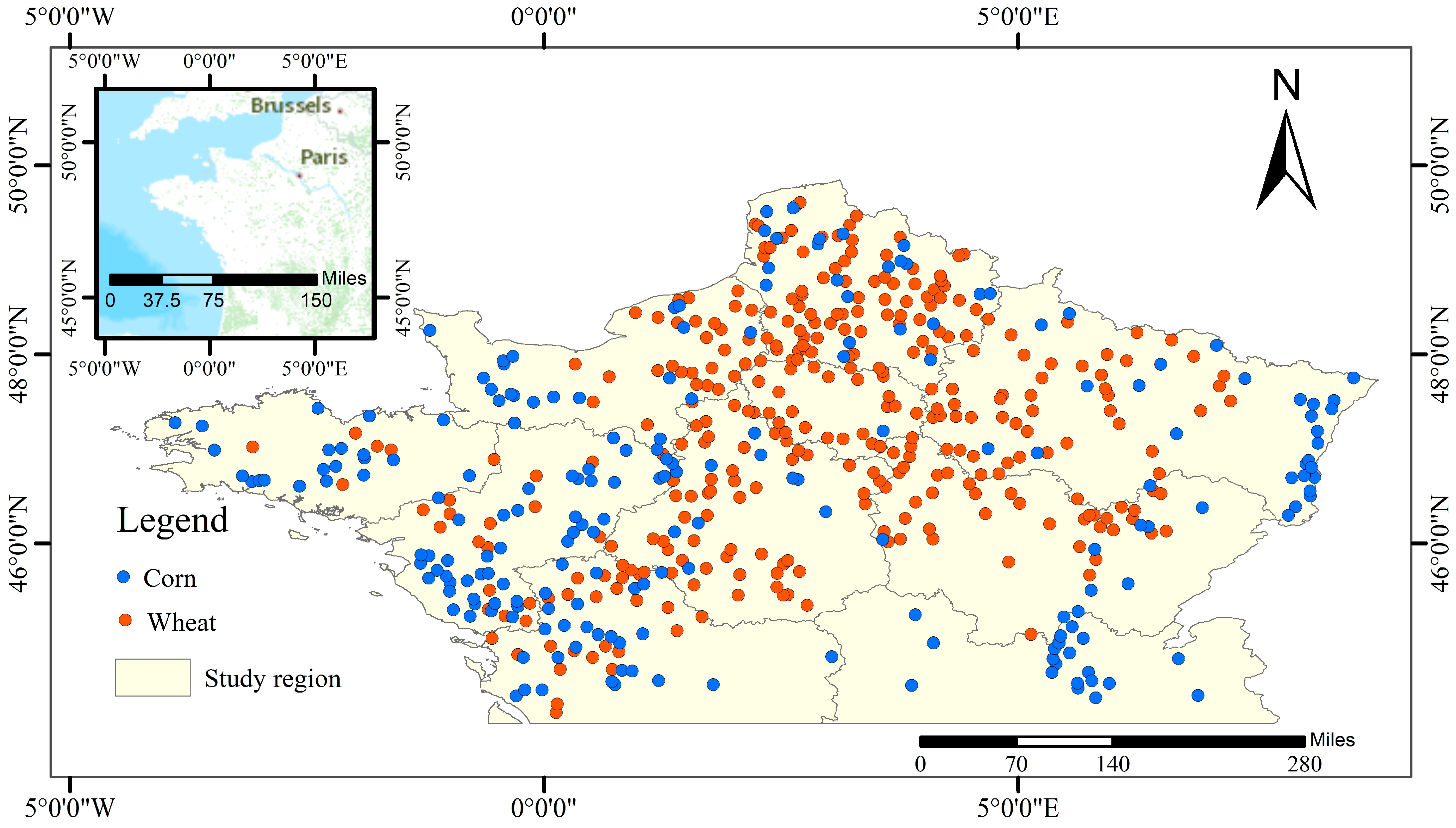
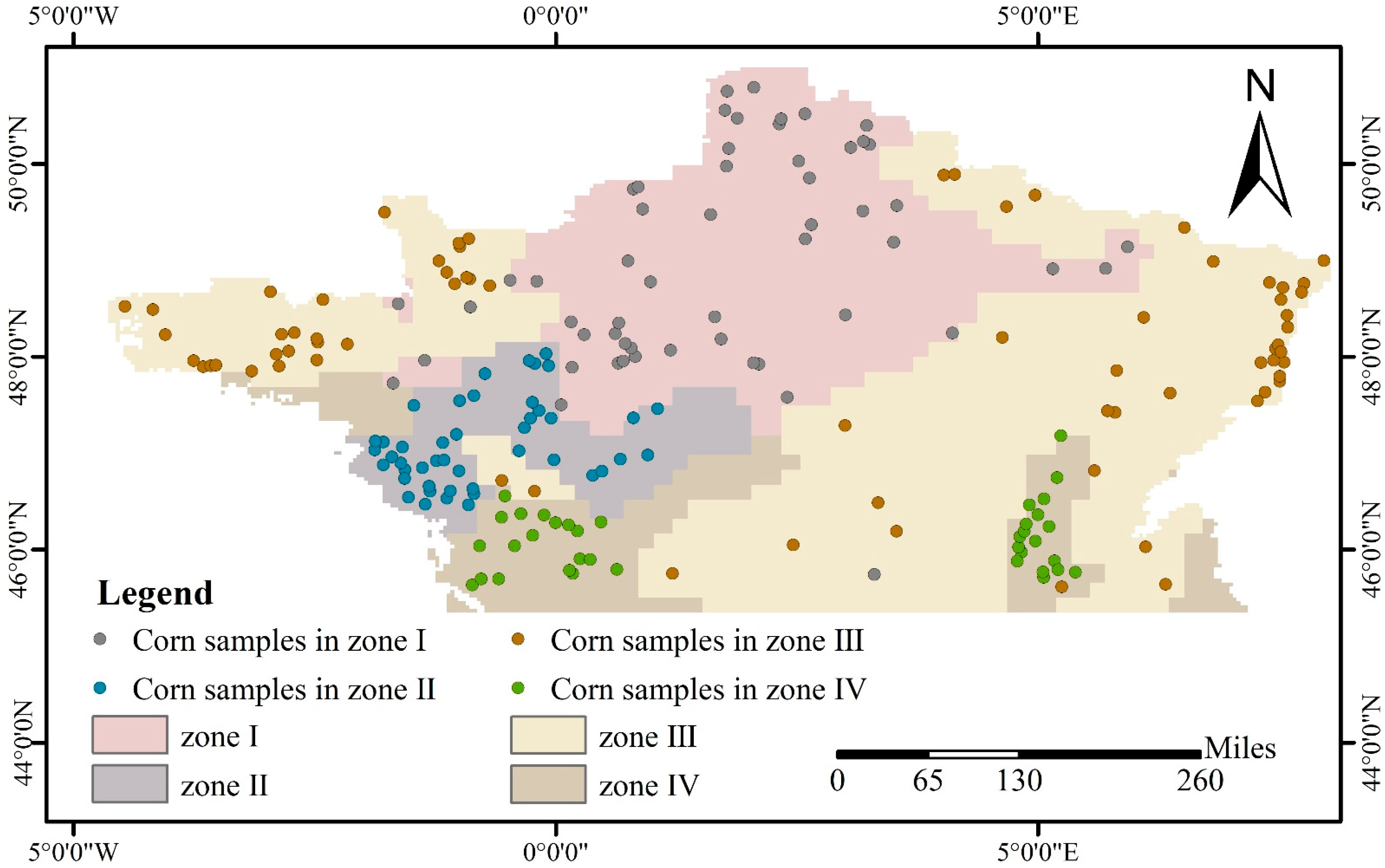
The study area is the northern part of the French mainland, excluding Corsica (Figure 1), which is relatively flat. This area experiences warm weather and some rains all year round and is thus suitable for the growth of various crops. Agriculture is well developed with a high degree of modernization. The main crops widely grown are wheat, corn, and sugar beet. Since France is an important supplier and exporter of agricultural and sideline products globally, efficient and accurate monitoring of crops in this region is essential.
2.2. Data Acquisition and Analysis
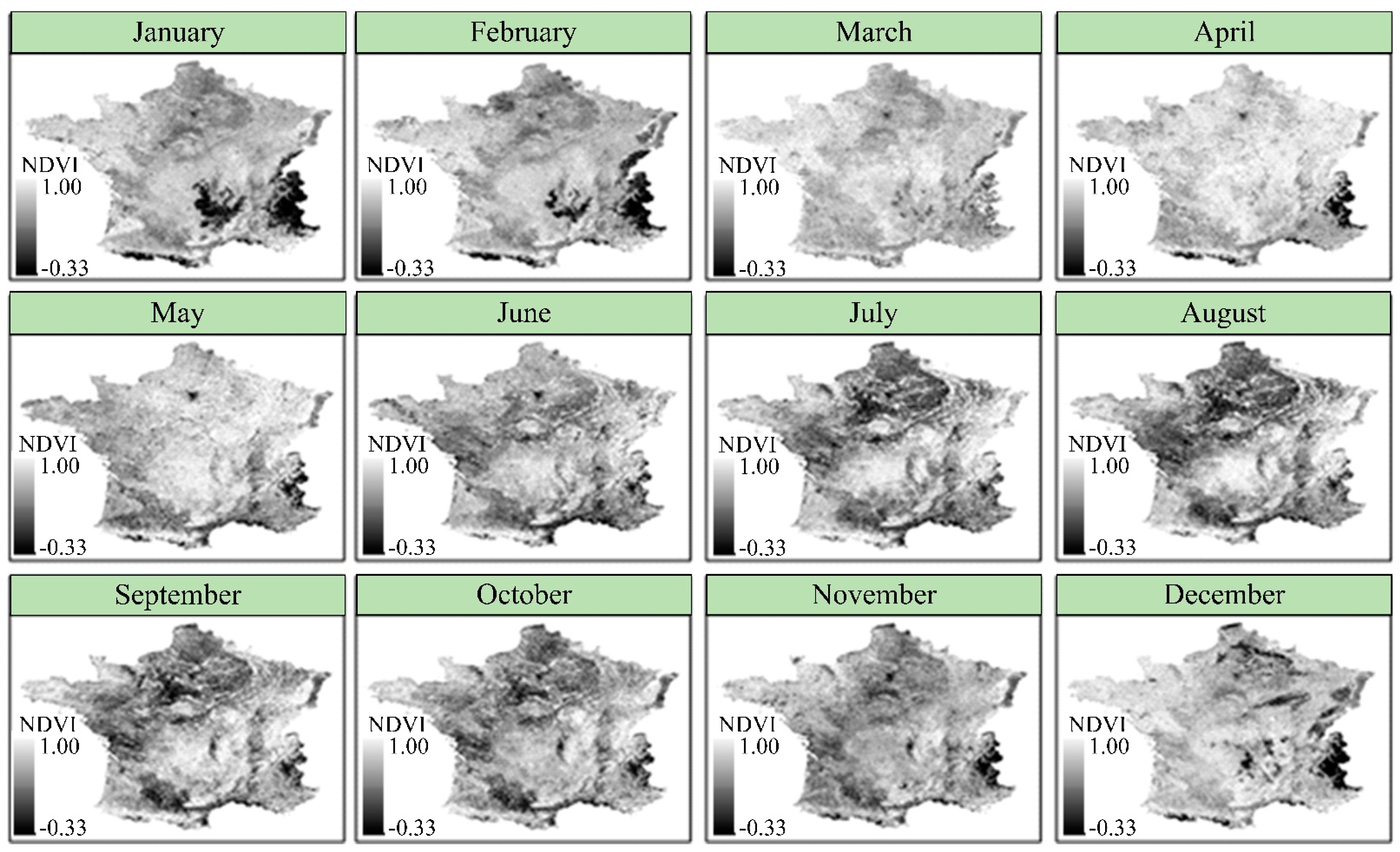
The sample dataset with crop types and geographical location information is derived from the 2009 European LUCAS dataset (Figure 1). Wheat and corn are the two main crops concentrated in northern France and are therefore used as the study crop types. For the study area, 325 wheat samples, 600 non-wheat samples, 213 corn samples, and 545 non-corn samples were obtained. The remote sensing data are obtained from the 2009 MODIS13Q1 product (Figure 2). The Savitzky–Golay smoothing filter is used to reduce noise and retain effective spectral information. The environmental data (topography, temperature, precipitation) are obtained from WorldClim [21] (https://www.worldclim.org/data/index.html (accessed on 29 November 2009)), where the monthly average image data are selected for climate and precipitation. The spatial resolution is 2.5 min (~12 km2).
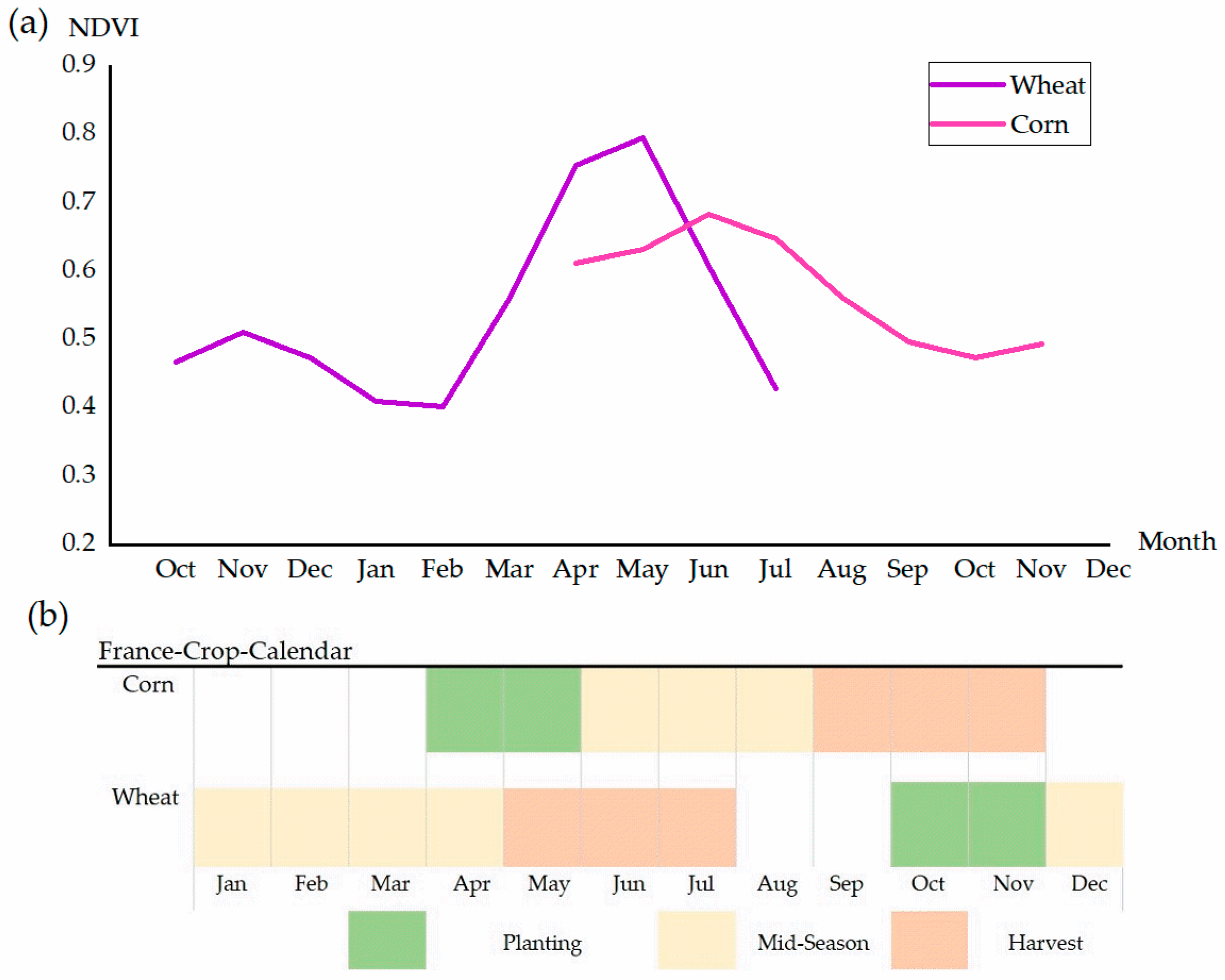
Phenology refers to the cyclical changes of crops in response to external environmental conditions. The varying phenological information and growth characteristics among crops are the key to their differentiation. The relevant phenological information on crops in the study area is obtained through a series of previous studies [22,23,24]. Figure 3 shows that the growth cycle of wheat is from October to July, and corn is from April to November. These months of the growth cycle must be included in the calculation of classification indexes.
3. Methodology
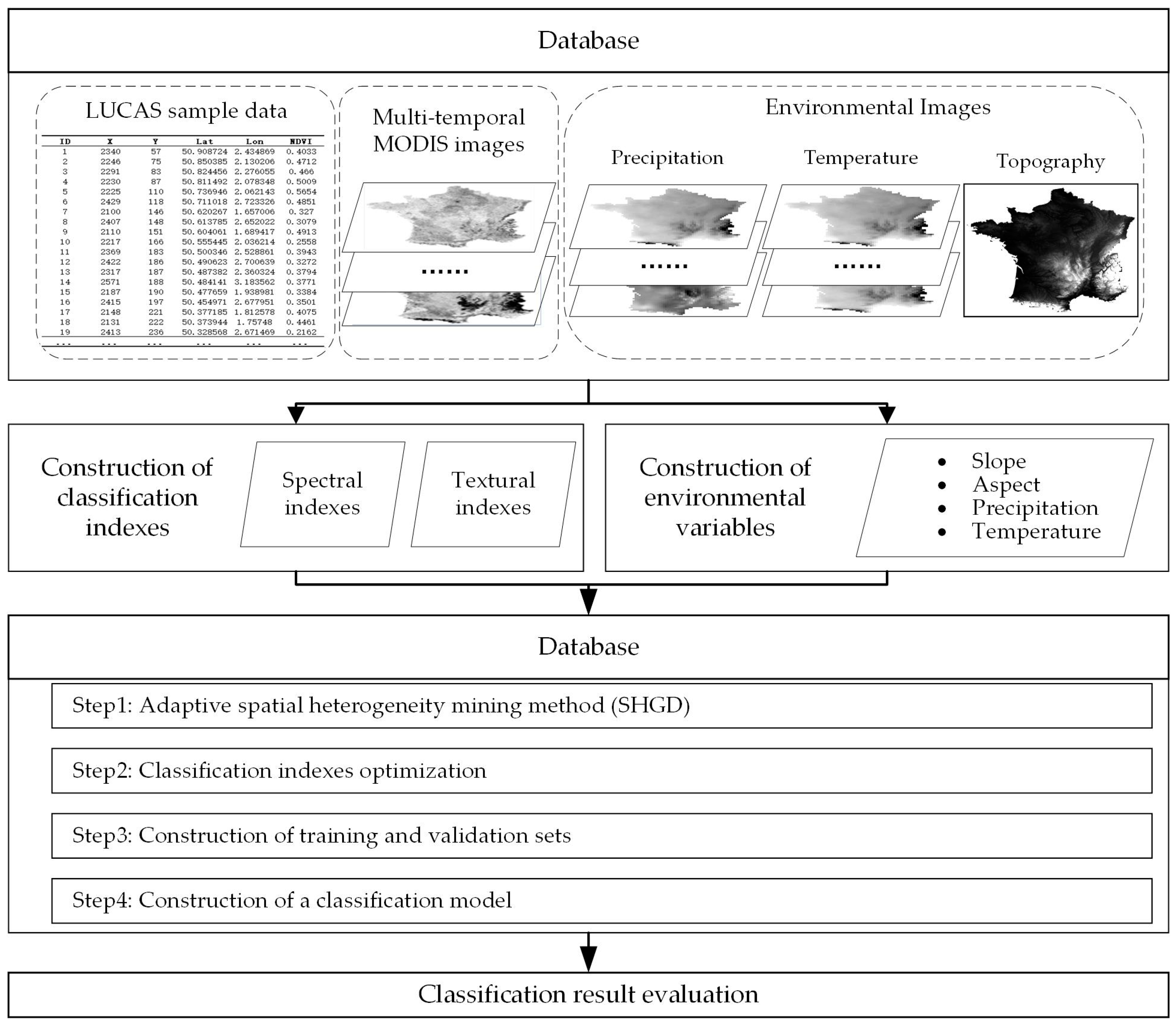
Spectral and textural indexes that can characterize crop features are discussed in Section 3.1. Environmental variables related to spatial heterogeneity are given in Section 3.2. The proposed ACCSH to classify crops is explained in Section 3.3. The classification evaluation indicators for assessing the classification effect are described in Section 3.4. The procedure is given in Figure 4.
3.1. Construction of Classification Indexes
3.1.1. Construction of Spectral Indexes
The MODIS13Q1 product captures images across five bands, including NDVI, red, blue, near-infrared (NIR), and middle-infrared (MIR), which were adopted as spectral indexes for 12 months in 2009. Additionally, different growth characteristics between crops are mainly reflected in the NDVI time series curves (Figure 3) in terms of spectral information [25,26,27]. Two quantitative indexes [26,27], curve trend and curve difference , are proven to be effective to distinguish different crops. and are then calculated based on the NDVI values of crop phenology according to the equations in Table 1. reflects the fluctuating trend of crop growth change and measures the correlation with the pseudo phenology curves [26]. High means more similarities between the sample and the target crop. measures the distance difference with the pseudo phenology curves and judges the difference between curves [27]. Low indicates a small difference between sample and the target crop. In summary, spectral bands, and were used as spectral indexes in this study.
3.1.2. Construction of Textural Indexes
As a commonly used texture algorithm, a gray-level co-occurrence matrix [28] was adopted to calculate textural indexes based on the images in Figure 2. Textural indexes include the mean, variance, homogeneity, contrast, dissimilarity, entropy, second moment, and correlation (Table 2). The mean reflects the relationship between the brightness of the target pixel and its neighbors. Variance indicates the degree of grayscale variation in the local area of the image. Homogeneity shows the concentration of pixels in the matrix. The contrast reflects the degree of gray difference in the local area. Dissimilarity is the linear correlation of the contrast of pixels in the local area. Entropy was used to measure the textural information, and the richer the textural information, the larger the entropy value. The second moment was used to describe the distribution of image brightness. Correlation reflects the interrelation between the target pixel and its neighbors, and the correlation is strong if the interdependence is large.
3.2. Construction of Environmental Variables
The crop growth characteristics significantly vary under different environmental conditions. In the study area, the main environmental variables [29,30] affecting crop growth were as follows: (1) temperature, (2) precipitation, (3) slope, and (4) aspect (see Table 3). Temperature and precipitation were downloaded from WorldClim 2 [21]. Slope and aspect were calculated on the basis of the Shuttle Radar Topography Mission [31]. Details of data processing and calculation of environmental variables were obtained from previous studies [32,33].
3.3. ACCSH Method
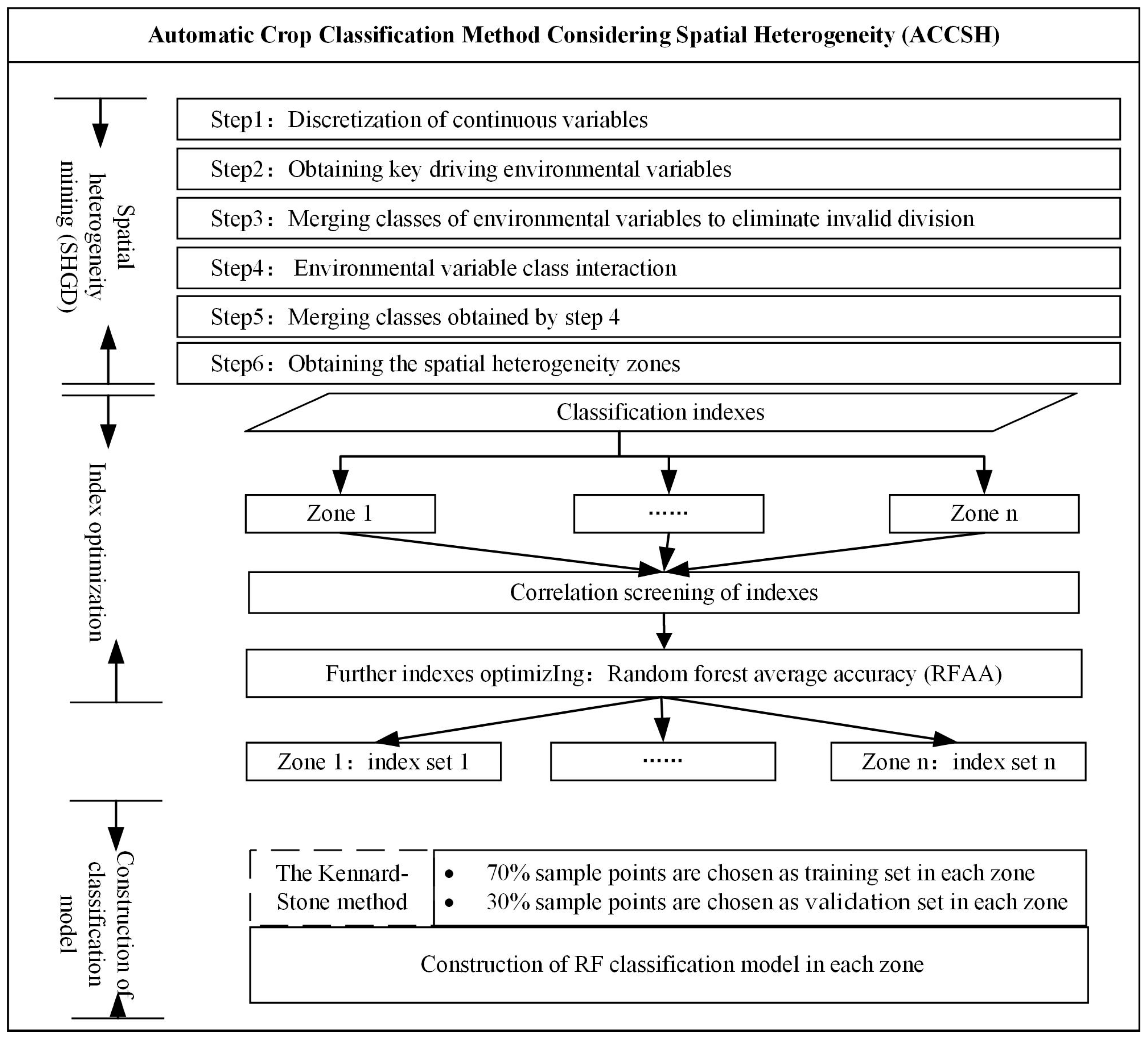
This study proposed an ACCSH, which consists of three separate phases, as described below in Section 3.3.1, Section 3.3.2 and Section 3.3.3. Phase 1 aims to mine the spatial heterogeneity patterns of crop growth characteristics under the effects of multiple environmental variables. An adaptive spatial heterogeneity mining method (SHGD) presented in Section 3.3.1 was put forward on the basis of the geographical detector technique. In Phase 2, the classification indexes were optimized. As the crop growth characteristics differ in each spatial homogeneous zone obtained via SHGD, the key indexes for classification vary from zone to zone. Therefore, a separate index optimization in each spatial homogeneous zone must be performed to obtain effective classification indexes and reduce data redundancy. The optimization strategy is described in Section 3.3.2. In Phase 3, we constructed the classification model while considering the spatial heterogeneity, as explained in Section 3.3.3. The procedure is given in Figure 5.
3.3.1. Spatial Heterogeneity Patterns Mining
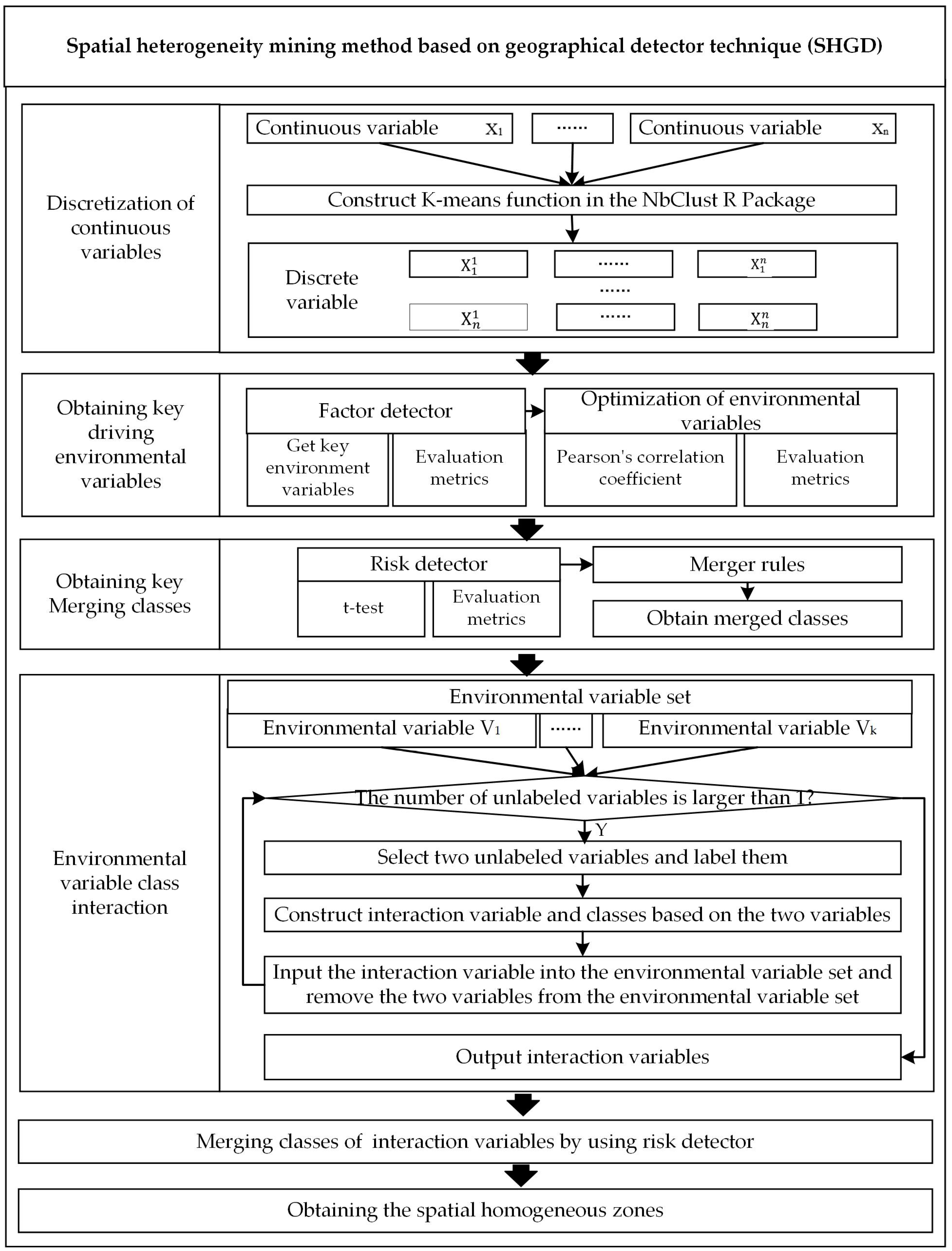
The geographical detector technique was proven effective for mining the spatial heterogeneity patterns under the effects of driving variables [10,11], but only discrete variables were suitable. Additionally, with numerous driving variables and categories, the spatial homogeneous zones may be too broken, which is inconvenient for subsequent classification operations. We addressed the abovementioned problems using an improved SHGD. The flow chart of SHGD is given in Figure 6, and its detailed procedure is as follows:
Step 1: Discretize continuous variables.
Environment variables driving the spatial heterogeneity of crops are mainly continuous measurements. The K-means method can segment continuous variables into several classes with similar intra-class distributions and different inter-class distributions. However, the number of classes in this method needed to be set. The NbClust package, which was developed to choose the optimal number of clusters for the dataset, was verified to be effective [34,35]. Hence, this study used the K-means function in the NbClust R package to obtain the optimal discrete categories.
Step 2: Determine key driving environmental variables.
The factor detector of the GD was adopted to mine the key driving environmental variables. However, highly correlated driving environmental variables need optimization. The detailed operations are as indicated below.
Step 2.1: In Equation (1), environmental variables are labeled as and the main classification index measuring crop growth characteristics is set as . Temporal NDVI can quantify crop growth characteristics to a large extent [36,37], and therefore, the mean NDVI of crop phenology is calculated as in Equation (1). The environmental variables with a significant p-value less than 0.05 of q in Equation (1) are selected as key factors using the GD [38].
where is the number of potential driving environmental variables ; is the class number of the environment variable ; is the number of samples in class of ; are the variance of in the area of class of ; is the variance of in the whole region; and and are the within and the total sum of squares, respectively. The value range of is [0, 1], and a large indicates the strong ability to reveal the spatial heterogeneity of .
Step 2.2: Environmental variables are optimized. The Pearson’s correlation coefficients between key factors obtained in step 2.1 were calculated. Two variables with a Pearson’s correlation coefficient larger than 0.8 and a significance value smaller than 0.05 were regarded as highly correlated [39]. If two variables are highly correlated, only the variable with higher q-statistic significance in the GD result is retained. The reserved variables are labeled as .
Step 3: Merge classes of environmental variables to eliminate invalid division.
If classes and simultaneously meet the following rule, they can be merged.
Rule: Classes and are from the same environmental variable. in class is similar to that in class , which can be measured using a t-test value of the risk detector of the GD result.
Step 4: Interaction of environmental variables. The detailed procedure is as follows.
Step 4.1: Classes in are labeled as .
Step 4.2: Select two variables and to construct interactive classes. and can be interacted with as new classes . is placed into , and and are deleted from .
Step 4.3: Go to step 4.2. The procedure is continued until only one element remains in .
Step 5: Merge classes obtained by step 4. The difference of between classes in is assessed using the t-test value of the risk detector of the GD result. Classes with no significant difference of are merged.
Step 6: Calculate the spatial homogeneous zones. Locations of classes that remain after step 5 are the eventual spatial homogeneous zones , where is their number. In these zones, have remarkable differences driven by multiple environmental variables. That is, crop growth characteristics significantly differ between zones, and the samples were extracted for the following independent classification operation.
3.3.2. Index Optimization
Index optimization is generally carried out from two aspects. The first is to reduce the redundancy of indexes, commonly performed by assessing Pearson’s correlation coefficient. The second is to retain importance indexes to improve the efficiency of the classification model. RFAA is one of the typical methods for retaining importance indexes. RFAA can provide a feature ranking based on the contribution of each feature and selects optimal indexes by measuring the change in model performance when the order of each feature is disrupted. RFAA has been widely used and proven effective for index optimization [40,41].
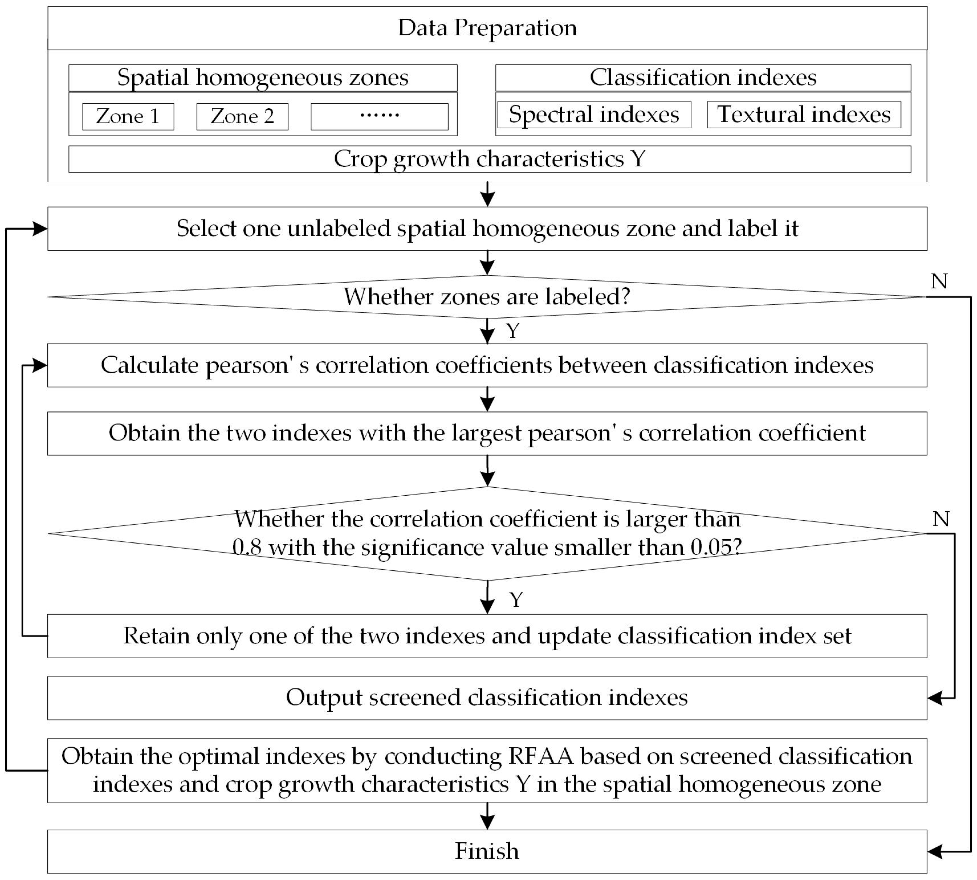
In this study, correlations may exist among the spectral and textural indexes of the crops and indicate that indexes contain duplicate information or are prone to redundancy. In addition, the growth characteristics between a particular crop and other types are concentrated on specific spectral or textural features in certain months. Therefore, to further effectively reduce redundancy and improve accuracy, we optimized the classification indexes using not only Pearson’s correlation coefficient but also RFAA. Additionally, given the distinct variabilities in crop growth characteristics within each spatial homogeneous zone, index optimization was carried out individually. The detailed procedure of the index optimization strategy is explained below (Figure 7).
Step 1: Select one unlabeled spatial homogeneous zone for labeling.
Step 2: Perform correlation screening of indexes.
A Pearson’s correlation analysis was carried out for spectral and textural indexes. The correlation between indexes was considered high when the coefficient was larger than 0.8, and the significance value was smaller than 0.05 [39]. When indexes were highly correlated, only one index was retained.
Step 3: Perform optimal classification index mining.
RFAA is widely used in index screening, in which indexes are selected by measuring the variation of model performance when the order of each index is disrupted. Indexes were selected by evaluating their importance. The optimal combination of indexes can contribute the most to crop classification and was retained [42,43].
Step 4: Go to step 1 until classification indexes in all spatial homogeneous zones are optimized. Optimized indexes in each spatial homogeneous zone were saved and used for the following operations.
3.3.3. Classification Model Construction
The crop growth characteristics differ between spatial homogeneous zones, and the main indexes distinguishing between crop types vary in each spatial homogeneous zone. Hence, the crop classification must be separately carried out in each spatial homogeneous zone.
RF is a comprehensive learning algorithm based on decision trees, which has been widely used in various classification and regression fields [44,45]. The RF classification model was constructed using the training set in each spatial homogeneous zone based on the optimized indexes. The classification accuracy was evaluated using the validation set in each separate spatial homogeneous zone. The validation set construction strategy and classification evaluation indexes are given in Section 3.4.
3.4. Accuracy Evaluation
The Kennard–Stone (KS) algorithm can effectively select the training and validation sets with sufficient regional representation of classification indexes and was adopted in this study [46]. Among the sample crops, 70% were chosen as the training set, and the remaining 30% were utilized as the validation set [47]. The classification performance was eventually evaluated using the kappa coefficient, F1 score, and accuracy, which are commonly used and verified to be effective [48]. The F1 score is aimed at dichotomies and reflects the classification effect of target-type crops, which is the harmonic value of recall and precision. Additionally, accuracy signifies the percentage of the correctly predicted rate of the whole sample [49]. The kappa coefficient is a comprehensive index to evaluate the classification performance of the model as a whole.
4. Results
Wheat and corn are two crop types used in this study, and the classification results using ACCSH are given in Section 4.1 and Section 4.2, respectively.
4.1. Crop Classification of Wheat
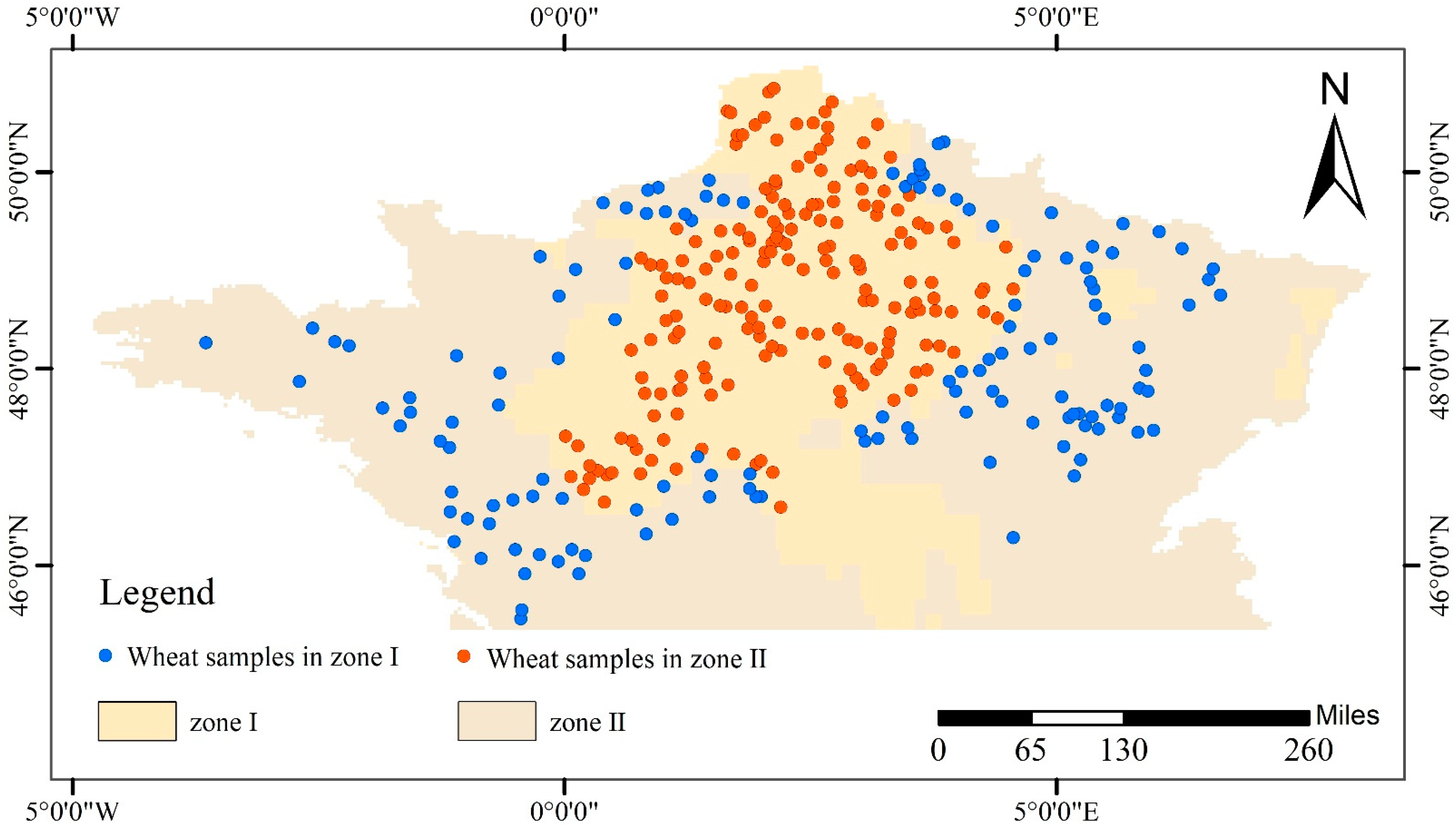
The SHGD in ACCSH is used to mine the spatial heterogeneity patterns of wheat. The mean NDVI is used as Y in Equation (1). Factor detection using steps 1 and 2 of SHGD indicates that , which is divided into three classes, has a significant effect on the spatial heterogeneity characteristics of wheat growth (Table 4). Risk detection using step 3 of SHGD in Table 5 indicates that the crop growth characteristics of wheat in classes 2 and 3 of have no significant difference. As such, classes 2 and 3 of can be combined as shown in Table 6, and the whole area is divided into spatial homogeneous zones I and II, respectively (Table 6 and Figure 8).
According to Section 3.1, spectral and textural indexes during the phenological period (Figure 3) are calculated for wheat classification. The index optimization strategy described in Section 3.3.2 is carried out on the spectral and textural indexes. The results in Table 7 show that the optimal index sets of wheat vary within each spatial homogeneous zone, further verifying the necessity of index optimization.
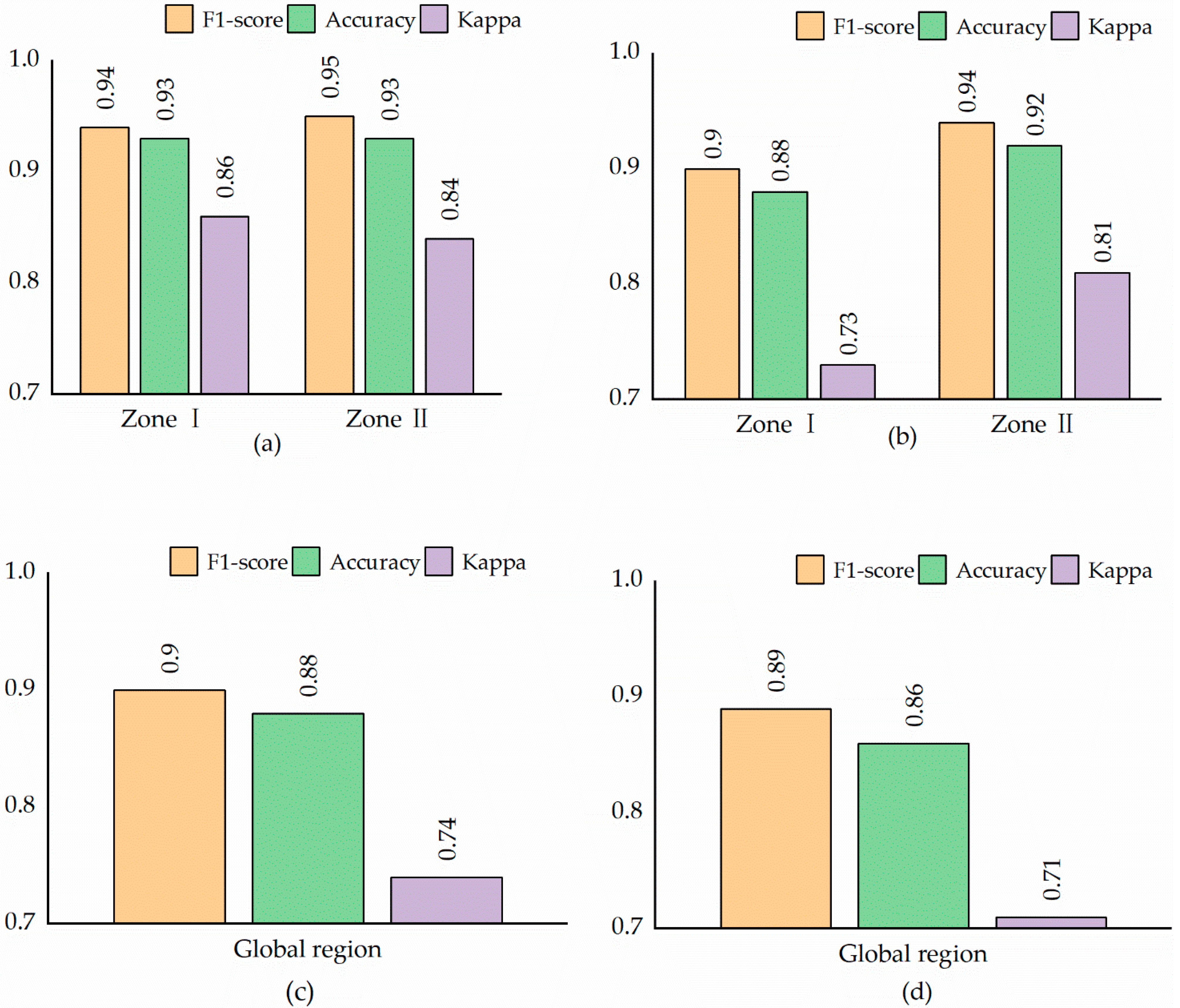
The ACCSH based on the optimized classification indexes is carried out, and the corresponding classification evaluation indicators are shown in Figure 9. The ACCSH in zones I and II show F1 scores of 0.94 and 0.95, respectively; the values of classification accuracy are 0.93 and 0.93, respectively, and the kappa coefficients are 0.86 and 0.84, respectively. The evaluation indicators indicate that ACCSH exhibits high stability and classification ability and can be utilized to classify wheat in a large-scale region with significant spatial heterogeneity.
4.2. Crop Classification of Corn
SHGD is used to mine the spatial heterogeneity patterns, and the mean NDVI of corn during the phenological period is used as in Equation (1). The results indicate that and can be divided into three classes using K-means. Then, key driving environmental variables are obtained, and both and show significant effects (p < 0.05) on the spatial heterogeneity of corn growth characteristics according to the factor detection result in Table 8. According to step 3 of SHGD, the risk detection results are given in Table 9 and Table 10, respectively, and classes of and are optimized as classes in Table 11 and Table 12, respectively, and are further interacted according to step 4. The risk detection of interaction classes is subsequently executed (Table 13), which manifests their remarkable variation in crop growth characteristics. Therefore, the locations of interaction classes are considered as the eventual spatial homogeneous zones (Table 14 and Figure 10).
Spectral and textural indexes of corn during its phenological period are calculated according to methods in Section 3.1. Similar to the results for wheat, the optimized classification indexes in spatial homogeneous zones and global areas vary (Table 15), setting barriers to the high accuracy of crop classification at the global scale.
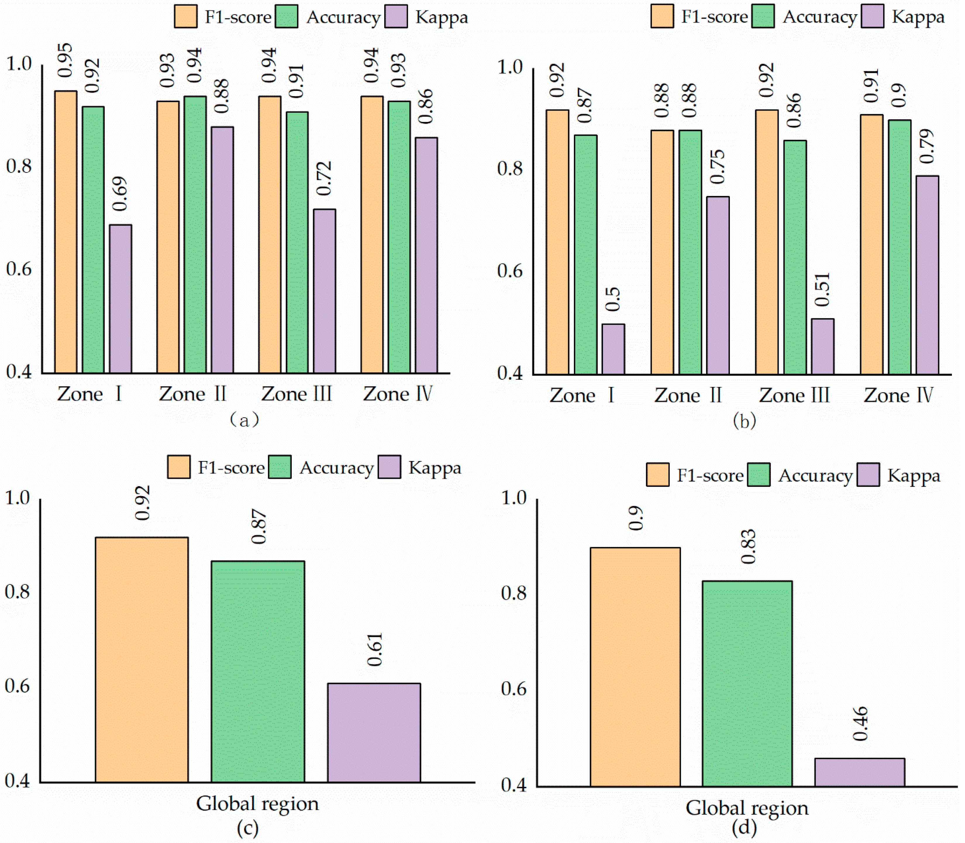
Figure 11 presents the classification evaluation indicators of corn. Results show that the F1 scores and accuracy indicators of ACCSH in zones I–IV are all higher than 0.9, verifying its effective crop classification ability with high accuracy in a large-scale region with significant spatial heterogeneity.
5. Discussion
5.1. Comparison Results of ACCSH with Classical Methods for Crop Classification
The classification effectiveness of ACCSH’s zoning strategy is further verified by comparison at the global scale; that is, the classification is constructed using RF combined with optimized classification indexes at the global scale in the study area. The validity of the index optimization operation can be verified using ACCSH and ACCSH with non-optimized indexes. Additionally, one of the widely used deep learning methods, the 1D Convolutional Neural Network (1D-CNN), is used for comparison. The comparative results are given and analyzed below.
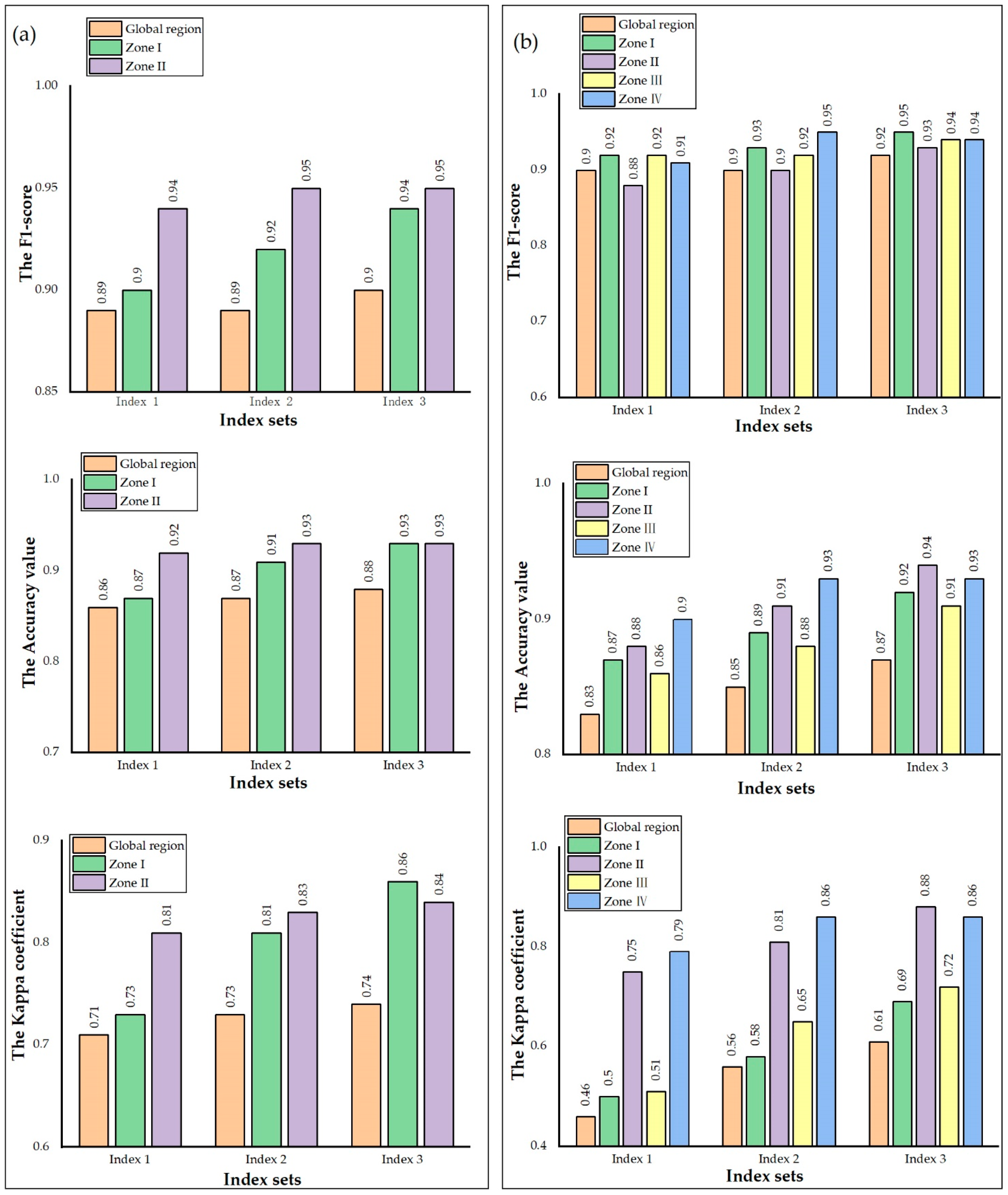
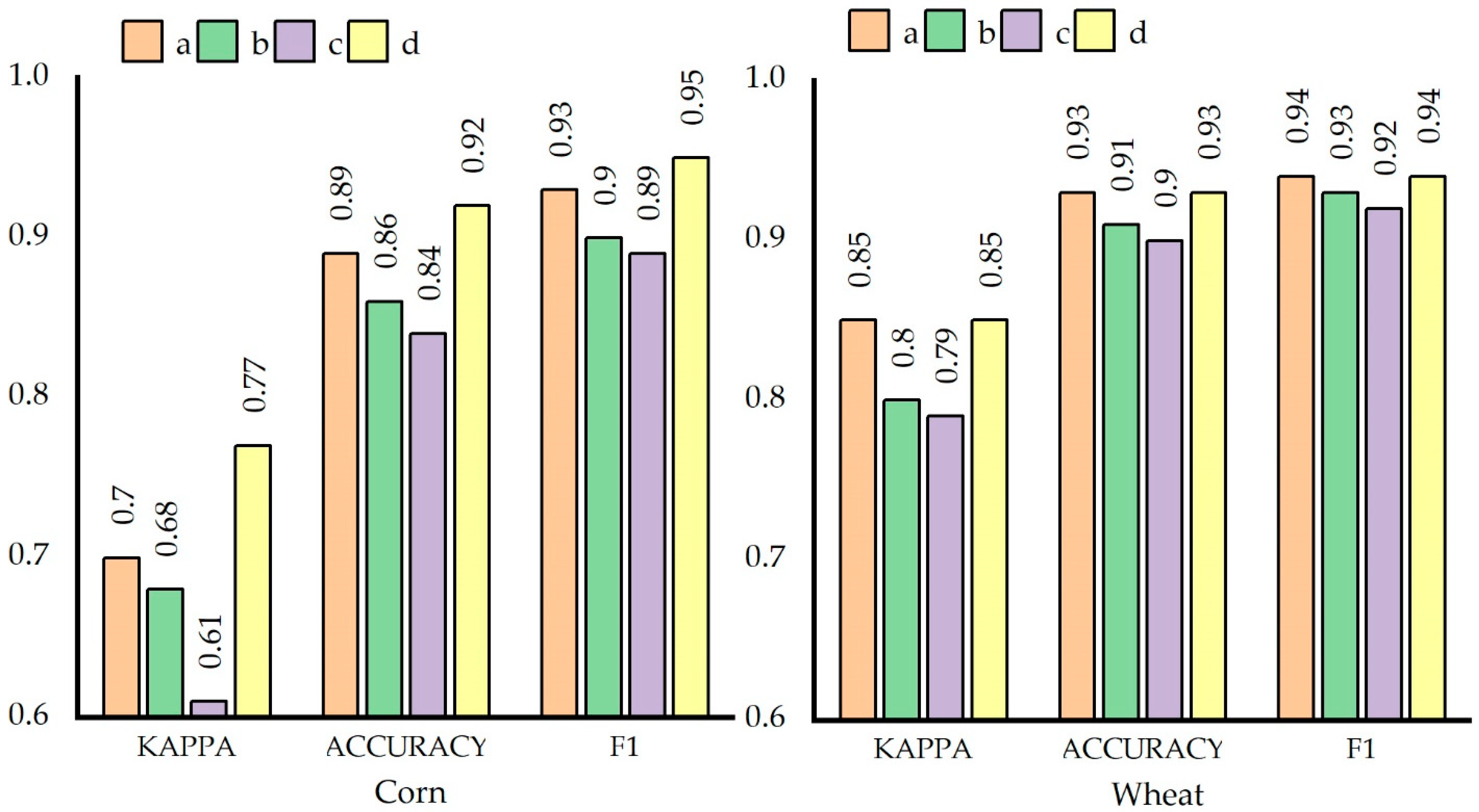
Figure 12a shows the evaluation indicators of wheat. The results show that the kappa coefficients of ACCSH in zones I and II are 16% and 14% higher than that of the classification at the global scale, respectively. Figure 12b presents the classification evaluation indicators of corn. The results show that the kappa coefficients of ACCSH in zones I–IV are all higher than those at the global scale. Thus, Figure 12 indicates that the index optimization strategy combining correlation screening and RFAA in Section 3.3.2 can effectively improve crop classification accuracy. Classification based on an index set optimized using correlation screening can improve the accuracy compared with that based on a non-optimized index set. Accuracy can be further improved based on the index set optimized using correlation screening followed by RFAA, and the index optimization strategy is adopted in ACCSH as described in Section 3.3.2. The index optimization strategy adopted in ACCSH can improve the kappa coefficient of classification effect by 5–18% for wheat and 9–42% for corn. The combination of correlation screening and the RFAA index optimization strategy can effectively screen the key classification indexes. In summary, the index optimization and spatial zoning strategies of ACCSH can improve crop classification. The kappa coefficient of ACCSH is improved by 20–67%, and the F1 score of ACCSH is improved by 6% compared with that of the global classification and classification based on non-optimized index sets, respectively. The ACCSH can perform crop classification with relatively high ability and can meet actual demand in large areas with significant spatial heterogeneity.
The kappa coefficients of wheat and corn using 1D-CNN classification are 0.72 and 0.58, respectively, which are significantly lower than those of ACCSH. The possible reason is that the training of deep learning models requires a large number of datasets [50,51]. When the sample size is limited, the machine learning-based ACCSH can achieve a relatively good classification accuracy.
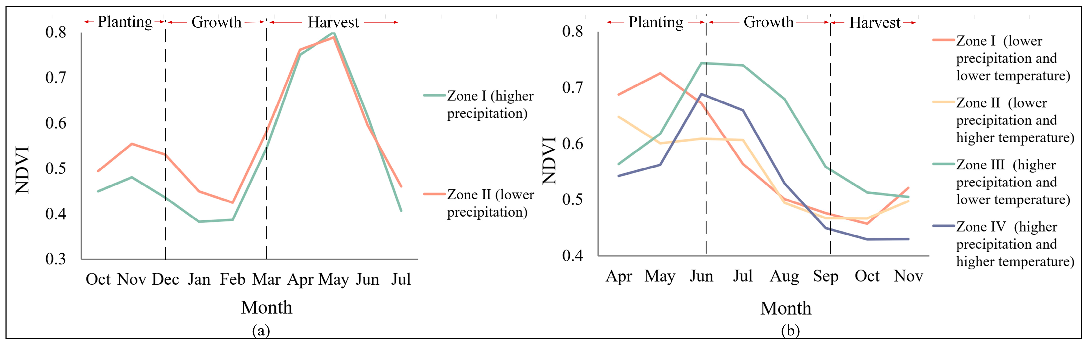
5.2. Analysis of the Spatial Heterogeneity Patterns of Crop Growth
According to Section 4.1, precipitation has a significant effect on wheat growth. The mean annual precipitation in zone II is higher than that in zone I (Table 4), and the mean NDVI value of wheat in zone II is higher than that in zone I during the planting and growth period of wheat (Figure 13a). That is, in the study area, precipitation has a positive driving effect on wheat growth, which may be the reason why a certain level of high precipitation results in better soil moisture reserves, contributing to better conditions. According to Section 4.2, the growth characteristics of corn significantly vary within spatial homogeneous zones driven by precipitation and temperature (Figure 13b). The higher precipitation during the growth period of corn in zones III and IV causes better growth than in zones I and II, and this finding is highly consistent with the relationship between precipitation and wheat growth. Additionally, for corn, the higher temperature in zones II and IV reduces the NDVI values compared with zones I and III during the planting period. High temperature increases the evaporation of water and reduces humidity, resulting in difficulties for emerging seedlings and the water loss of pollen. The interaction of these two factors shows that the combination of high precipitation and low temperature in zone III contributes to the best corn growth, whereas the combination of low precipitation and high temperature are the worst conditions. In summary, SHGD in ACCSH can mine the spatial heterogeneous characteristics of crop growth. To further demonstrate the efficacy of SHGD, we use the typical layered approaches, such as that based on management zones [7,8] and on segmented single climatic variables (i.e., temperature or precipitation) in place of SHGD in the ACCSH. The results in Figure 14 indicate that ACCSH based on SHGD has the highest classification accuracy, demonstrating its power to mine spatial heterogeneous patterns for crop classification. Specifically, the best wheat zoning outcome depends on the precipitation segmentation that SHGD adaptively mines.
In summary, ACCSH can be effectively applied to crop classification in large areas, and the proposed SHGD can mine the driving effects of multiple environmental variables on the spatial heterogeneity of crop growth characteristics.
6. Conclusions
This study proposes ACCSH to automatically classify crops considering the spatial heterogeneity of crop growth characteristics under the influence of multiple environmental factors. Experiments on two real applications are carried out. Comprehensive comparisons are designed, including classifications at the global scale and based on non-optimized classification indexes. The proposed ACCSH has the following advantages: (1) The results of SHGD in ACCSH can reveal the spatial homogeneous zones and mechanism of crop growth characteristics under the influence of multiple environmental variables. (2) The index optimization strategy in ACCSH can fully consider the differences between spatial homogeneous zones by carrying out a separate optimization in each spatial homogeneous zone and obtaining the key classification indexes to improve classification accuracy. (3) ACCSH can automatically perform crop classification without sufficient prior knowledge of the study area.
ACCSH is used for wheat and corn classification in northern France. The following new findings are obtained from the study: (1) The influence of the mean annual precipitation on wheat is significantly positive. The better condition for wheat growth is due to relatively high precipitation; (2) Corn growth is sensitive to both precipitation and temperature, where the former exhibits an overall positive driving effect, whereas the latter tends to have a negative effect on crop growth; (3) The accuracies of ACCSH evaluated using the kappa coefficient are 15% for wheat and 26% for corn, higher than those of classification at the global scale; (4) The accuracies of ACCSH are also much higher than those of classifications based on non-optimized classification indexes.
Overall, ACCSH can automatically carry out crop classification under the influence of multiple environmental factors on crop growth, indicating its potential in crop classification with relatively high precision. In addition, ACCSH is adaptive and implemented using R 4.3.0 software and Matlab 2014a software, which makes the operation convenient. Future research can focus on the application and improvement of the ACCSH. The proposed method is suitable for single crop classification, and future studies can improve ACCSH to adapt to multiple and rotation crop classifications. Additionally, if sufficient remote sensing data with high spatial resolution are available, ACCSH can be carried out at a small scale.
Author Contributions
X.W., P.P. and S.H. conceived and designed the experiments; X.W., S.H. and K.Y. performed the experiments; Y.C. collected data; all the authors analyzed the data; X.W. wrote the paper; all authors contributed to the revision of the manuscript. All authors have read and agreed to the published version of the manuscript.
Funding
This research was funded by the National Natural Science Foundation of China, grant number [42101474], and the Guizhou Provincial Science and Technology Project, grant number (qiankehezhicheng [2023] general 238).
Data Availability Statement
The data presented in this study are openly available upon request.
Conflicts of Interest
The authors declare no conflict of interest. Y.C. was employed by the company Guizhou Zhiyuan Engineering Technology Consulting Co., Ltd. The remaining authors declare that the research was conducted in the absence of any commercial or financial relationships that could be construed as a potential conflict of interest.”
References
- Kuang, X.; Guo, J.; Bai, J.; Geng, H.; Wang, H. Crop-Planting Area Prediction from Multi-Source Gaofen Satellite Images Using a Novel Deep Learning Model: A Case Study of Yangling District. Remote Sens. 2023, 15, 3792. [Google Scholar] [CrossRef]
- Zhang, L.; Gao, L.; Huang, C.; Wang, N.; Wang, S.; Peng, M.; Zhang, X.; Tong, Q. Crop classification based on the spectrotemporal signature derived from vegetation indices and accumulated temperature. Int. J. Digit. Earth 2022, 15, 626–652. [Google Scholar] [CrossRef]
- Song, W.; Feng, A.; Wang, G.; Zhang, Q.; Dai, W.; Wei, X.; Hu, Y.; Amankwah, S.O.Y.; Zhou, F.; Liu, Y. Bi-Objective Crop Mapping from Sentinel-2 Images Based on Multiple Deep Learning Networks. Remote Sens. 2023, 15, 3417. [Google Scholar] [CrossRef]
- Hao, Y.Y.; Luo, X.B.; Zhong, B.; Yang, A.X. Methods of the National Vegetation Classification Based on Vegetation Partition. In Proceedings of the 4th International Conference on Mechanical Materials and Manufacturing Engineering, Wuhan, China, 15–16 October 2016. [Google Scholar]
- He, P.; Xu, X.; Zhang, B.; Li, Z.; Jin, X.; Zhang, Q.; Zhang, Y. Crop Classification Extraction Based on Multi-temporal GF-1 Remote Sensing Image. J. Henan Agric. Sci. 2016, 45, 152–159. [Google Scholar] [CrossRef]
- Aparecido, L.; Rolim, G.; Moraes, J.; Rocha, H.; Lense, G.; Souza, P. Agroclimatic zoning for urucum crops in the state of Minas Gerais, Brazil. Bragantia 2017, 77, 193–200. [Google Scholar] [CrossRef]
- Chen, H.; Wang, X.; Zhang, W.; Wang, X.Z.; Di, X.D.; Qi, L.Q. A New Soybean Ndvi Data-Based Partitioning Algorithm for Fertilization Management Zoning. Appl. Ecol. Environ. Res. 2021, 19, 1391–1405. [Google Scholar] [CrossRef]
- Santos, S.G.; Melo, J.C.; Constantino, R.G.; Brito, A.V. A Solution for Vegetation Analysis, Separation and Geolocation of Management Zones using Aerial Images by UAVs. In Proceedings of the IX Brazilian Symposium on Computing Systems Engineering (SBESC), Natal, Brazil, 19–22 November 2019. [Google Scholar]
- Wang, J.; Li, X.; Christakos, G.; Liao, Y.; Zhang, T.; Gu, X.; Zheng, X. Geographical Detector“ Based Health Risk Assessment and its Application in the Neural Tube Defects Study of the Heshun Region, China. Int. J. Geogr. Inf. Sci. 2010, 24, 107–127. [Google Scholar] [CrossRef]
- Zhu, L.; Meng, J.; Zhu, L. Applying Geodetector to disentangle the contributions of natural and anthropogenic factors to NDVI variations in the middle reaches of the Heihe River Basin. Ecol. Indic. 2020, 117, 106545. [Google Scholar] [CrossRef]
- Meng, X.; Gao, X.; Li, S.; Lei, J. Spatial and Temporal Characteristics of Vegetation NDVI Changes and the Driving Forces in Mongolia during 1982–2015. Remote Sens. 2020, 12, 603. [Google Scholar] [CrossRef]
- Han, Y.; Guo, X.; Jiang, Y.; Xu, Z.; Li, Z. Environmental factors influencing spatial variability of soil total phosphorus content in a small watershed in Poyang Lake Plain under different levels of soil erosion. Catena 2020, 187, 104357. [Google Scholar] [CrossRef]
- Nidamanuri, R.R.; Zbell, B. Use of field reflectance data for crop mapping using airborne hyperspectral image. ISPRS J. Photogramm. Remote Sens. 2011, 66, 683–691. [Google Scholar] [CrossRef]
- Gerstmann, H.; Möller, M.; Gläßer, C. Optimization of spectral indices and long-term separability analysis for classification of cereal crops using multi-spectral RapidEye imagery. Int. J. Appl. Earth Obs. Geoinf. 2016, 52, 115–125. [Google Scholar] [CrossRef]
- Waldhoff, G.; Lussem, U.; Bareth, G. Multi-Data Approach for remote sensing-based regional crop rotation mapping: A case study for the Rur catchment, Germany. Int. J. Appl. Earth Obs. Geoinf. 2017, 61, 55–69. [Google Scholar] [CrossRef]
- Ciriza, R.; Sola, I.; Albizua, L.; Álvarez-Mozos, J.; González-Audícana, M. Automatic Detection of Uprooted Orchards Based on Orthophoto Texture Analysis. Remote Sens. 2017, 9, 492. [Google Scholar] [CrossRef]
- Numbisi, F.N.; Coillie, F.V.; Wulf, R.R.d. Delineation of Cocoa Agroforests Using Multiseason Sentinel-1 SAR Images: A Low Grey Level Range Reduces Uncertainties in GLCM Texture-Based Mapping. ISPRS Int. J. Geo Inf. 2019, 8, 179. [Google Scholar] [CrossRef]
- Kawamura, K.; Asai, H.; Yasuda, T.; Soisouvanh, P.; Phongchanmixay, S. Discriminating crops/weeds in an upland rice field from UAV images with the SLIC-RF algorithm. Plant Prod. Sci. 2020, 24, 198–215. [Google Scholar] [CrossRef]
- Xie, Q.; Lai, K.; Wang, J.; Lopez-Sanchez, J.M.; Shang, J.; Liao, C.; Zhu, J.; Fu, H.; Peng, X. Crop Monitoring and Classification Using Polarimetric RADARSAT-2 Time-Series Data Across Growing Season: A Case Study in Southwestern Ontario, Canada. Remote Sens. 2021, 13, 1394. [Google Scholar] [CrossRef]
- Akbari, E.; Boloorani, A.D.; Samany, N.N.; Hamzeh, S.; Soufizadeh, S.; Pignatti, S. Crop Mapping Using Random Forest and Particle Swarm Optimization based on Multi-Temporal Sentinel-2. Remote Sens. 2020, 12, 1449. [Google Scholar] [CrossRef]
- Fick, S.E.; Hijmans, R.J.J.I.J.o.C. WorldClim 2: New 1-km spatial resolution climate surfaces for global land areas. Int. J. Climatol. 2017, 37, 4302–4315. [Google Scholar] [CrossRef]
- Demarez, V.; Helen, F.; Marais-Sicre, C.; Baup, F. In-season mapping of irrigated crops using landsat 8 and sentinel-1 time series. Remote Sens. 2019, 11, 118. [Google Scholar] [CrossRef]
- Marais-Sicre, C.; Inglada, J.; Fieuzal, R.; Baup, F.; Valero, S.; Cros, J.; Huc, M.; Demarez, V.J.R.S. Early detection of summer crops using high spatial resolution optical image time series. Remote Sens. 2016, 8, 591. [Google Scholar] [CrossRef]
- Veloso, A.; Mérmoz, S.; Bouvet, A.; Toan, T.L.; Planells, M.; Dejoux, J.-F.; Ceschia, E. Understanding the temporal behavior of crops using sentinel-1 and sentinel-2-like data for agricultural applications. Remote Sens. Environ. 2017, 199, 415–426. [Google Scholar] [CrossRef]
- Jiang, M.; Xin, L.; Li, X.; Tan, M.; Wang, R. Decreasing Rice Cropping Intensity in Southern China from 1990 to 2015. Remote Sens. 2018, 11, 35. [Google Scholar] [CrossRef]
- Meero, F.v.d.; Bakker, W.H. Cross correlogram spectral matching: Application to surface mineralogical mapping by using AVIRIS data from Cuprite, Nevada. Remote Sens. Environ. 1997, 61, 371–382. [Google Scholar] [CrossRef]
- Guo, Y.; Liu, Q.; Liu, G.; Huang, C. Research on extraction of planting information of major crops based on MODIS time-series NDVI. J. Nat. Resour. 2017, 32, 1808–1818. [Google Scholar]
- Park, Y.; Guldmann, J.-M. Measuring continuous landscape patterns with Gray-Level Co-Occurrence Matrix (GLCM) indices: An alternative to patch metrics? Ecol. Indic. 2020, 109, 105802. [Google Scholar] [CrossRef]
- Worku, T.; Khare, D.; Tripathi, S.K. Spatiotemporal trend analysis of rainfall and temperature, and its implications for crop production. J. Water Clim. Chang. 2019, 10, 799–817. [Google Scholar] [CrossRef]
- Toreti, A.; Belward, A.S.; Pérez-Domínguez, I.; Naumann, G.; Luterbacher, J.; Cronie, O.; Seguini, L.; Manfron, G.; López-Lozano, R.; Baruth, B.; et al. The Exceptional 2018 European Water Seesaw Calls for Action on Adaptation. Earth’s Future 2019, 7, 652–663. [Google Scholar] [CrossRef]
- Rabus, B.T.; Eineder, M.; Roth, A.; Bamler, R. The shuttle radar topography mission—A new class of digital elevation models acquired by spaceborne radar. ISPRS J. Photogramm. Remote Sens. 2003, 57, 241–262. [Google Scholar] [CrossRef]
- Perrin, G.; Rapinel, S.; Hubert-Moy, L.; Bioret, F. Bioclimatic dataset of Metropolitan France under current conditions derived from the WorldClim model. Data Brief 2020, 31, 105815. [Google Scholar] [CrossRef]
- Vangansbeke, P.; Máliš, F.; Hédl, R.; Chudomelová, M.; Vild, O.; Wulf, M.; Jahn, U.; Welk, E.; Rodríguez-Sánchez, F.; De Frenne, P. ClimPlant: Realized climatic niches of vascular plants in European forest understoreys. Glob. Ecol. Biogeogr. 2021, 30, 1183–1190. [Google Scholar] [CrossRef]
- Charrad, M.; Ghazzali, N.; Boiteau, V.; Niknafs, A. NbClust: An R Package for Determining the Relevant Number of Clusters in a Data Set. J. Stat. Softw. 2014, 61, 1–36. [Google Scholar] [CrossRef]
- Et-taleby, A.; Boussetta, M.; Benslimane, M. Faults Detection for Photovoltaic Field Based on K-Means, Elbow, and Average Silhouette Techniques through the Segmentation of a Thermal Image. Int. J. Photoenergy 2020, 2020, 7. [Google Scholar] [CrossRef]
- Ji, S.; Zhang, C.; Xu, A.; Shi, Y.; Duan, Y. 3D Convolutional Neural Networks for Crop Classification with Multi-Temporal Remote Sensing Images. Remote Sens. 2018, 10, 75. [Google Scholar] [CrossRef]
- Zhang, H.; Kang, J.; Xu, X.; Zhang, L.-p. Accessing the temporal and spectral features in crop type mapping using multi-temporal Sentinel-2 imagery: A case study of Yi’an County, Heilongjiang province, China. Comput. Electron. Agric. 2020, 176, 105618. [Google Scholar] [CrossRef]
- Liu, Y.; Chen, Y.; Wu, Z.; Wang, B.; Wang, S. Geographical detector-based stratified regression kriging strategy for mapping soil organic carbon with high spatial heterogeneity. CATENA 2021, 196, 104953. [Google Scholar] [CrossRef]
- Dong, Z.; Men, Y.; Liu, Z.; Li, J.; Ji, J. Application of chlorophyll fluorescence imaging technique in analysis and detection of chilling injury of tomato seedlings. Comput. Electron. Agric. 2020, 168, 105109. [Google Scholar] [CrossRef]
- Chen, L.; Xing, M.; He, B.; Wang, J.; Shang, J.; Huang, X.; Xu, M. Estimating Soil Moisture Over Winter Wheat Fields During Growing Season Using Machine-Learning Methods. IEEE J. Sel. Top. Appl. Earth Obs. Remote Sens. 2021, 14, 3706–3718. [Google Scholar] [CrossRef]
- Elavarasan, D.; Vincent, P.M.D.R.; Srinivasan, K.; Chang, C.-Y. A Hybrid CFS Filter and RF-RFE Wrapper-Based Feature Extraction for Enhanced Agricultural Crop Yield Prediction Modeling. Agriculture 2020, 10, 400. [Google Scholar] [CrossRef]
- Reif, D.M.; Motsinger-Reif, A.A.; McKinney, B.A.; Crowe, J.E.; Moore, J.H. Feature Selection using a Random Forests Classifier for the Integrated Analysis of Multiple Data Types. In Proceedings of the IEEE Symposium on Computational Intelligence and Bioinformatics and Computational Biology, Toronto, ON, Canada, 28–29 September 2006; pp. 1–8. [Google Scholar] [CrossRef]
- Mahdianpari, M.; Mohammadimanesh, F.; Mcnairn, H.; Davidson, A.A.; Rezaee, M.; Salehi, B.; Homayouni, S. Mid-season Crop Classification Using Dual-, Compact-, and Full-Polarization in Preparation for the Radarsat Constellation Mission (RCM). Remote Sens. 2019, 11, 1582. [Google Scholar] [CrossRef]
- Xu, F.; Li, Z.; Zhang, S.; Huang, N.; Quan, Z.; Zhang, W.; Liu, X.; Jiang, X.; Pan, J.; Prishchepov, A.V. Mapping Winter Wheat with Combinations of Temporally Aggregated Sentinel-2 and Landsat-8 Data in Shandong Province, China. Remote Sens. 2020, 12, 2065. [Google Scholar] [CrossRef]
- Ge, X.; Wang, J.; Ding, J.; Cao, X.; Zhang, Z.; Liu, J.; Li, X. Combining UAV-based hyperspectral imagery and machine learning algorithms for soil moisture content monitoring. PeerJ 2019, 7, e6926. [Google Scholar] [CrossRef]
- Galvão, R.K.H.; Araújo, M.C.U.d.; José, G.E.; Pontes, M.J.C.; Silva, E.C.; Saldanha, T.C.B. A method for calibration and validation subset partitioning. Talanta 2005, 67, 736–740. [Google Scholar] [CrossRef] [PubMed]
- Wang, Y.; Wu, X.; Chen, Z.; Ren, F.; Feng, L.; Du, Q. Optimizing the Predictive Ability of Machine Learning Methods for Landslide Susceptibility Mapping Using SMOTE for Lishui City in Zhejiang Province, China. Int. J. Environ. Res. Public Health 2019, 16, 368. [Google Scholar] [CrossRef] [PubMed]
- Zhang, W.; Liu, H.; Wu, W.; Zhan, L.-Q.; Wei, J. Mapping Rice Paddy Based on Machine Learning with Sentinel-2 Multi-Temporal Data: Model Comparison and Transferability. Remote Sens. 2020, 12, 1620. [Google Scholar] [CrossRef]
- He, S.; Peng, P.; Chen, Y.; Wang, X.-m. Multi-Crop Classification Using Feature Selection-Coupled Machine Learning Classifiers Based on Spectral, Textural and Environmental Features. Remote Sens. 2022, 14, 3153. [Google Scholar] [CrossRef]
- Coltin, B.; McMichael, S.T.; Smith, T.; Fong, T. Automatic boosted flood mapping from satellite data. Int. J. Remote Sens. 2016, 37, 1015–1993. [Google Scholar] [CrossRef]
- Reyes, A.K.; Caicedo, J.C.; Camargo, J.E. Fine-tuning Deep Convolutional Networks for Plant Recognition. CLEF 2015, 1391, 467–475. [Google Scholar]
Figure 1.
Study region.

Figure 2.
Preprocessed remote sensing data with NDVI value.

Figure 3.
Phenological information of target crops. (a) is the pseudo phenology curve of the target crop, and the pseudo phenology curve is obtained by calculating the mean NDVI value of the crop sample points; (b) is the growth information of crops for each month.
Figure 3.
Phenological information of target crops. (a) is the pseudo phenology curve of the target crop, and the pseudo phenology curve is obtained by calculating the mean NDVI value of the crop sample points; (b) is the growth information of crops for each month.

Figure 4.
Workflow of crop classification.

Figure 5.
The process of ACCSH.

Figure 6.
The detailed procedure of SHGD.

Figure 7.
The detailed procedure of the index optimization strategy.

Figure 8.
Spatial homogeneous zones of wheat.

Figure 9.
Wheat classification effects under different classification strategies with RF classifier. (a) Result of ACCSH; (b) zoning results based on non-optimized index sets; (c) global result based on optimized index set; and (d) global result based on non-optimized index set.
Figure 9.
Wheat classification effects under different classification strategies with RF classifier. (a) Result of ACCSH; (b) zoning results based on non-optimized index sets; (c) global result based on optimized index set; and (d) global result based on non-optimized index set.

Figure 10.
Spatial homogeneous zones of corn.

Figure 11.
Corn classification effects under different classification strategies with RF classifier. (a) Result of ACCSH; (b) zoning results based on non-optimized index sets; (c) global result based on optimized index set; and (d) global result based on non-optimized index set.
Figure 11.
Corn classification effects under different classification strategies with RF classifier. (a) Result of ACCSH; (b) zoning results based on non-optimized index sets; (c) global result based on optimized index set; and (d) global result based on non-optimized index set.

Figure 12.
Evaluation indicators of wheat and corn classifications under different index optimization strategies. (a) is the classification evaluation indicator of wheat; (b) is the classification evaluation indicator of corn. Index 1 is the non-optimized index set. Index 2 is the correlation screening index set. Index 3 is the optimized index set using the strategy in ACCSH.

Figure 13.
Growth characteristics of wheat and corn under different spatial homogeneous zones. (a) is the mean NDVI of wheat during the phenological period in each spatial homogeneous zone, and (b) is the mean NDVI of corn during the phenological period in each spatial homogeneous zone.
Figure 13.
Growth characteristics of wheat and corn under different spatial homogeneous zones. (a) is the mean NDVI of wheat during the phenological period in each spatial homogeneous zone, and (b) is the mean NDVI of corn during the phenological period in each spatial homogeneous zone.

Figure 14.
Crop classification based on the following layered method: (a) segmented precipitation method; (b) segmented temperature method; (c) management zone method; and (d) SHGD.
Figure 14.
Crop classification based on the following layered method: (a) segmented precipitation method; (b) segmented temperature method; (c) management zone method; and (d) SHGD.


Table 1.
Spectral indexes and interpretation.
| Indicator | Calculation Formula | Meanings |
|---|---|---|
| -NDVI | - | The NDVI value in month . |
| -RED | - | The value of red band in month . |
| -BLUE | - | The value of blue band in month . |
| n-NIR | - | The value of NIR band in month . |
| n-MIR | - | The value of MIR band in month . |
| Similarity between sample and crop type in NDVI index, is the target crop. | ||
| Difference between sample and crop type in the NDVI index, is the target crop. |
is the label of the classified sample; is the average NDVI value of samples of crop type during the phenological period of crop type . represents the average NDVI value of the crop type in the month . is the label of each month during the phenological period of crop type . is the average NDVI value of sample during the phenological period of crop type , and represents the NDVI value of sample in the month . Time phase number in this study is calculated using the phenological period of crop .
Table 2.
Textural indexes and interpretation.
| Index | Meaning |
|---|---|
| The value of textural index mean in month | |
| The value of textural index variance in month | |
| The value of textural index homogeneity in month | |
| The value of textural index homogeneity in month | |
| The value of textural index dissimilarity in month | |
| The value of textural index entropy in month | |
| The value of textural index second moment in month | |
| The value of textural index correlation in month |
is calculated using the phenological period of the target crop. When the target crop is wheat, }; when the target crop is corn, .
Table 3.
Environmental indicators highly related to crop growth.
| Index | Meaning |
|---|---|
| Slope | Degree of surface inclination |
| Aspect | Orientation of the topographic slope |
| Mean precipitation during phenological period | |
| Mean temperature during phenological period |
Table 4.
Factor detection result using the GD model for wheat classification.
| Statistical Variable | Aspect | Slope | ||
|---|---|---|---|---|
| q statistic | 0.10 | 0.01 | 0.01 | 0.00 |
| p-value | 0.00 | 0.14 | 0.43 | 0.94 |
Table 5.
Risk detection result of classes of using the GD model for wheat classification.
| Classes | Class 1 | Class 2 | Class 3 |
|---|---|---|---|
| class 1 | |||
| class 2 | Y | ||
| class 3 | Y | N |
Y represents the remarkably different crop growth characteristics between classes and vice versa anti.
Table 6.
Optimized classes of for wheat classification.
| Classes | Optimized Classes | Values | Spatial Homogeneous Zones |
|---|---|---|---|
| class 1 | A | between 43.0 and 57.0 | I |
| class 2 | B | between 57.0 and 68.8 | II |
| class 3 | B | between 68.8 and 109.6 | II |
Table 7.
Optimized classification indexes of wheat.
| Region | Index Type | Index Name |
|---|---|---|
| Global region | Spectral indexes | 1-NDVI, 5-NDVI, 7-NDVI, 8-NDVI |
| 5-BLUE, 8-BLUE | ||
| 7-NIR,12-NIR | ||
| 8-MIR | ||
| , | ||
| Textural indexes | 6-B4, 7-B4, 12-B4 | |
| 12-B5 | ||
| 7-B6 | ||
| 6-B7 | ||
| Zone I | Spectral indexes | 3-NDVI, 4-NDVI, 5-NDVI, 7-NDVI, 8-NDVI |
| 10-RED | ||
| 4-NIR | ||
| 5-MIR | ||
| , | ||
| Textural indexes | 8-B1 | |
| 9-B2 | ||
| 10-B6 | ||
| 9-B8, 12-B8 | ||
| Zone II | Spectral indexes | 5-NDVI, 7-NDVI, 8-NDVI |
| 7-RED, 8-RED, 9-RED | ||
| 8-BLUE, 9-BLUE | ||
| 8-MIR, 9-MIR | ||
| , | ||
| Textural indexes | 7-B1, 8-B1 | |
| 7-B4, 8-B4 | ||
| 7-B6, 8-B6 | ||
| 8-B7, 9-B7 |
Table 8.
Factor detection result using the GD model for corn classification.
| Statistical Variable | Aspect | Slope | ||
|---|---|---|---|---|
| q statistic | 0.01 | 0.04 | 0.02 | 0.00 |
| p-value | 0.02 | 0.02 | 1.00 | 0.83 |
Table 9.
Risk detection result of classes of using the GD model for corn classification.
| Classes | Class 1 | Class 2 | Class 3 |
|---|---|---|---|
| class 1 | |||
| class 2 | Y | ||
| class 3 | Y | N |
Table 10.
Risk detection result of classes of using the GD model for corn classification.
| Classes | Class 1 | Class 2 | Class 3 |
|---|---|---|---|
| class 1 | |||
| class 2 | N | ||
| class 3 | N | Y |
Table 11.
Optimized classes of for corn classification.
| Classes | Optimized Classes | Values |
|---|---|---|
| 1 | C | between 48.5 and 60 |
| 2 | D | between 60 and 71.8 |
| 3 | D | between 71.8 and 95.5 |
Table 12.
Optimized classes of for corn classification.
| Classes | Optimized Classes | Values |
|---|---|---|
| 1 | E | between 10.0 and 13.3 |
| 2 | E | between 13.3 and 14.2 |
| 3 | F | between 14.2 and 15.5 |
Table 13.
Risk detection result of interaction classes using the GD model for corn classification.
| Classes | Class 1 | Class 2 | Class 3 | Class 4 |
|---|---|---|---|---|
| class 1 | ||||
| class 2 | Y | |||
| class 3 | Y | Y | ||
| class 4 | Y | Y | Y |
Table 14.
Interaction classes of and for corn classification.
| Classes | Interaction Information | Values | Spatial Homogeneous Zones |
|---|---|---|---|
| 1 | between 48.5 to 60 and between 10.0 and 13.3 | Zone I | |
| 2 | between 48.5 to 60 and between 14.2 and 15.5 | Zone II | |
| 3 | between 60 to 95.5 and between 10.0 and 14.2 | Zone III | |
| 4 | between 60 to 95.5 and between 14.2 and 15.5 | Zone IV |
Table 15.
Optimized classification indexes of corn.
| Region | Index Type | Index Name |
|---|---|---|
| Global region | Spectral indexes | 5-NDVI, 7-NDVI |
| 7-RED, 8-RED | ||
| 5-BLUE | ||
| 9-NIR | ||
| 5-MIR | ||
| , | ||
| Textural indexes | 5-B1, 6-B1, 12-B1 | |
| 7-B3 | ||
| 7-B7 | ||
| 6-B8 | ||
| Zone I | Spectral indexes | 5-NDVI, 7-NDVI, 8-NDVI |
| 5-RED, 8-RED | ||
| 5-MIR, 6-MIR | ||
| Textural indexes | 1-NDVI, 2-NDVI, 3-NDVI, 7-NDVI, 11-NDVI, 12-NDVI | |
| 2-B6 | ||
| 7-B7 | ||
| 4-B8, 6-B8 | ||
| Zone II | Spectral indexes | 5-NDVI, 6-NDVI, 7-NDVI, 8-NDVI |
| 7-RED | ||
| 7-BLUE, 8-BLUE | ||
| 7-NIR | ||
| 7-MIR | ||
| Textural indexes | 2-B1, 5-B1, 6-B1, 12-B1 | |
| 1-B2 | ||
| 2-B4 | ||
| 1-B6 | ||
| 1-B7 | ||
| Zone III | Spectral indexes | 11-NDVI |
| 5-RED, 7-RED, 8-RED | ||
| 4-BLUE, 5-BLUE, 8-BLUE | ||
| 7-NIR | ||
| 4-MIR, 5-MIR, 8-,MIR | ||
| Textural indexes | 5-B1 | |
| 2-B2 | ||
| Zone IV | Spectral indexes | 6-NDVI, 8-NDVI |
| 4-RED, 5-RED, 6-RED, 7-RED, 8-RED, 11-RED | ||
| 4-BLUE, 5-BLUE | ||
| 7-NIR | ||
| 5-MIR | ||
| Textural indexes | 3-B1, 7-B1 | |
| 7-B3 |
Disclaimer/Publisher’s Note: The statements, opinions and data contained in all publications are solely those of the individual author(s) and contributor(s) and not of MDPI and/or the editor(s). MDPI and/or the editor(s) disclaim responsibility for any injury to people or property resulting from any ideas, methods, instructions or products referred to in the content. |
© 2023 by the authors. Licensee MDPI, Basel, Switzerland. This article is an open access article distributed under the terms and conditions of the Creative Commons Attribution (CC BY) license (https://creativecommons.org/licenses/by/4.0/).
Share and Cite
MDPI and ACS Style
Wang, X.; Liu, J.; Peng, P.; Chen, Y.; He, S.; Yang, K. Automatic Crop Classification Based on Optimized Spectral and Textural Indexes Considering Spatial Heterogeneity. Remote Sens. 2023, 15, 5550. https://doi.org/10.3390/rs15235550
AMA Style
Wang X, Liu J, Peng P, Chen Y, He S, Yang K. Automatic Crop Classification Based on Optimized Spectral and Textural Indexes Considering Spatial Heterogeneity. Remote Sensing. 2023; 15(23):5550. https://doi.org/10.3390/rs15235550
Chicago/Turabian StyleWang, Xiaomi, Jiuhong Liu, Peng Peng, Yiyun Chen, Shan He, and Kang Yang. 2023. "Automatic Crop Classification Based on Optimized Spectral and Textural Indexes Considering Spatial Heterogeneity" Remote Sensing 15, no. 23: 5550. https://doi.org/10.3390/rs15235550
Note that from the first issue of 2016, this journal uses article numbers instead of page numbers. See further details here.