
Novel Grid Collection and Management Model of Remote Sensing Change Detection Samples
by
 , , , ,
Daoye Zhu
1,2,3,
Bing Han
2,
Elisabete A. Silva
3,
Shuang Li
4,
Min Huang
5,6,* ,
,
Fuhu Ren
2 and
Chengqi Cheng
2,7 1
College of Computer and Data Science, Fuzhou University, Fuzhou 350108, China
2
Center for Data Science, Peking University, Beijing 100871, China
3
Lab of Interdisciplinary Spatial Analysis, University of Cambridge, Cambridge CB3 9EP, UK
4
Institute of Chinese Historical Geography, Fudan University, Shanghai 200433, China
5
School of Geography and Environment, Jiangxi Normal University, Nanchang 330022, China
6
State Key Laboratory of Information Engineering in Surveying, Mapping and Remote Sensing, Wuhan University, Wuhan 430079, China
7
College of Engineering, Peking University, Beijing 100871, China
*
Author to whom correspondence should be addressed.
Remote Sens. 2023, 15(23), 5528; https://doi.org/10.3390/rs15235528
Submission received: 17 October 2023
/
Revised: 20 November 2023
/
Accepted: 23 November 2023
/
Published: 27 November 2023
(This article belongs to the Special Issue GeoAI and EO Big Data Driven Advances in Earth Environmental Science)
Abstract
:Remote sensing data have become an important data source for urban and regional change detection, owing to their advantages of authenticity, objectivity, immediacy, and low cost. The method of collection and management for remote sensing change detection samples (RS_CDS) assumes a crucial role in the effectiveness of remote sensing intelligent change detection (RSICD). To achieve rapid collection and real-time sharing of RS_CDS, this study proposes a grid collection and management model of RS_CDS based on GeoSOT (GCAM-GeoSOT), including the grid collection method of RS_CDS (GCM-SD) and grid management method of RS_CDS (GMM-SD). To verify the feasibility and retrieval efficiency of GMM-SD, Oracle and PostgreSQL databases were combined and the retrieval efficiency and database capacity were compared with the corresponding spatial databases, Oracle Spatial and PostgreSQL + PostGIS, respectively. The experimental results showed that GMM-SD not only ensures the reasonable capacity consumption of the database but also has a higher retrieval efficiency for the RS_CDS. This results in a noteworthy comprehensive performance enhancement, with a 47.63% improvement compared to Oracle Spatial and a 40.24% improvement compared to PostgreSQL + PostGIS.
1. Introduction
As urban complexes with highly dense populations, environments, and resources and intricate socio-economic factors, the sustainable development of cities must delimit a reasonable urban development boundary and optimize the spatial layout [1]. Land use/land cover (LULC) change detection is a critical problem in Earth observations, land use monitoring, urban expansion, and resource management [2,3,4,5]. Urban real-time monitoring, particularly the monitoring and management of illegal buildings, has important guiding significance for standardizing urban construction and reasonably guiding urban development. Remote sensing data have the advantages of authenticity, objectivity, immediacy, and low cost. Moreover, remote sensing has become an important data source for monitoring urban and regional management changes [6]. With recent advancements in the maturity of artificial intelligence technology such as deep learning, RSICD is proving more important for the management of urban and regional areas [7]. RSICD collects remote sensing change detection samples (RS_CDS) from remote sensing images in advance and compiles them into a comprehensive sample set. This set essentially determines the effect of RSICD, underscoring its pivotal role in the process. Consequently, the method of collection and management for RS_CDS assumes a crucial role in the effectiveness of RSICD.
At present, the collection methods of RS_CDS mainly include pixel-based sample collection and object-based sample collection. Pixel-based RSICD starts from the random initialization of parameters, requires a large number of training samples to train the network, and only extracts the spectral features of remote sensing images. The French National Institute of Information and Automation (INRIA) contains a large number of databases, and among them, the INRIA aerial image dataset [8] database is used for urban building detection, the training sets and datasets of which were collected from different urban remote sensing images, and only pixel-level buildings (not building marks) exist. In object-based RSICD sample collection, texture and shape features are applied to the feature expression of remote sensing images. For example, eCognition uses an object-based method to collect the RS_CDS. First, the image is segmented at multiple scales, and the segmented spots are used as the units for feature extraction. Texture and shape features are then added to the image features. The Houston 2018 dataset [9] has 20 types of LULC features, including 1,859,825 training samples and 321,729 test samples. The Berlin dataset [10,11] has eight types of LULC features, including 2820 training samples and 461,851 test samples. The MUUFL dataset [12] has 11 types of LULC features, including 1100 training samples and 53,687 test samples. In the collection and management of pixel-based and object-based RSICDs, there is a lack of standardized identification for the sample data, resulting in challenges for sharing both sample data and learning outcomes. Users also face difficulties in accurately accessing sample data at their desired locations. Additionally, considering the anticipated increase in the volume of RS_CDS in the future, the retrieval efficiency of conventional spatial databases is low.
Overall, the grid covers a wider range and contains more ground-object information. It is able to extract not only the spectral, texture, and shape features of a single object, but also the spatial topological relationship between multiple objects in the grid area. The spatial topological relationship is an important indicator of change, which can give full access to the ability of CNN to mine high-level features. Moreover, the grid feature vector can be constructed by combining grid image features and neighborhood grid information. Using the grid as the analysis unit of change detection allows for collection of large-scale urban statistics, structured proportions, and local changes, which is critical for urban planning.
Discrete Global Grid Systems (DGGS) is a global spatial reference system [13]. The system uses hierarchical grid cells that can completely embed the global surface to divide the Earth and describe its address information [14]. The important difference between DGGS and traditional spatial reference systems is that DGGS provides a digital framework for geospatial information [15]. Geospatial information is essentially a signal, which is a variable (such as the measurement of a phenomenon) that changes under the influence of another independent variable (such as spatial position, time, certain physical interactions). Traditional geospatial data are analog signals, as they are referenced by a continuous space of geographic coordinates on an ellipsoidal reference plane [16]. Even the discrete pixels of satellite Earth observation images refer to this continuous simulation model of the Earth. However, for continuous observation, these pixels cannot accurately observe the same location area. As the name suggests, DGGS provides sampling of position information based on regular discrete intervals or grid partitioning [15]. DGGS is mainly divided into an equal area Earth reference system (EA DGGS) and axis-aligned reference system (AA DGGS). EA DGGS has a global grid area of equal area, with each area having a unique identifier. However, as DGGS progresses toward 3D, 4D, and even higher dimensions, the existing equal product attributes will be greatly challenged [17]. In addition, AA DGGS can be divided based on whether the formation is parallel to the coordinate axis of the existing geographic information coordinate system, which is more flexible.
Spatial indexing has evolved significantly, incorporating cutting-edge methodologies such as the B+ tree, H3 index, R-tree, and generalized search tree (GIST). DataCube establishes field indexes using a B+ tree structure, where each B+ tree structure’s field index is equivalent to a data plane. That way, a global data table and its multiple important field indexes establish a data organization structure similar to a cube [18]. The H3 index is a hexagonal spatial index designed by Uber, which can obtain the boundaries of the H3 index hexagon using longitude and latitude. The corresponding hexagons for each longitude and latitude are determined [19]. Uber’s H3 index aggregates objects in geographical space using the H3 index, essentially converting longitude and latitude queries into H3 index queries. The R-tree index is a data structure designed for efficiently handling multidimensional data [20]. It proves invaluable for accessing spatial data, particularly when dealing with regional objects spanning two or more dimensions. GIST [21] allows the definition of a rule to distribute any type of data across a balanced tree and defines a method that uses this representation for operator access.
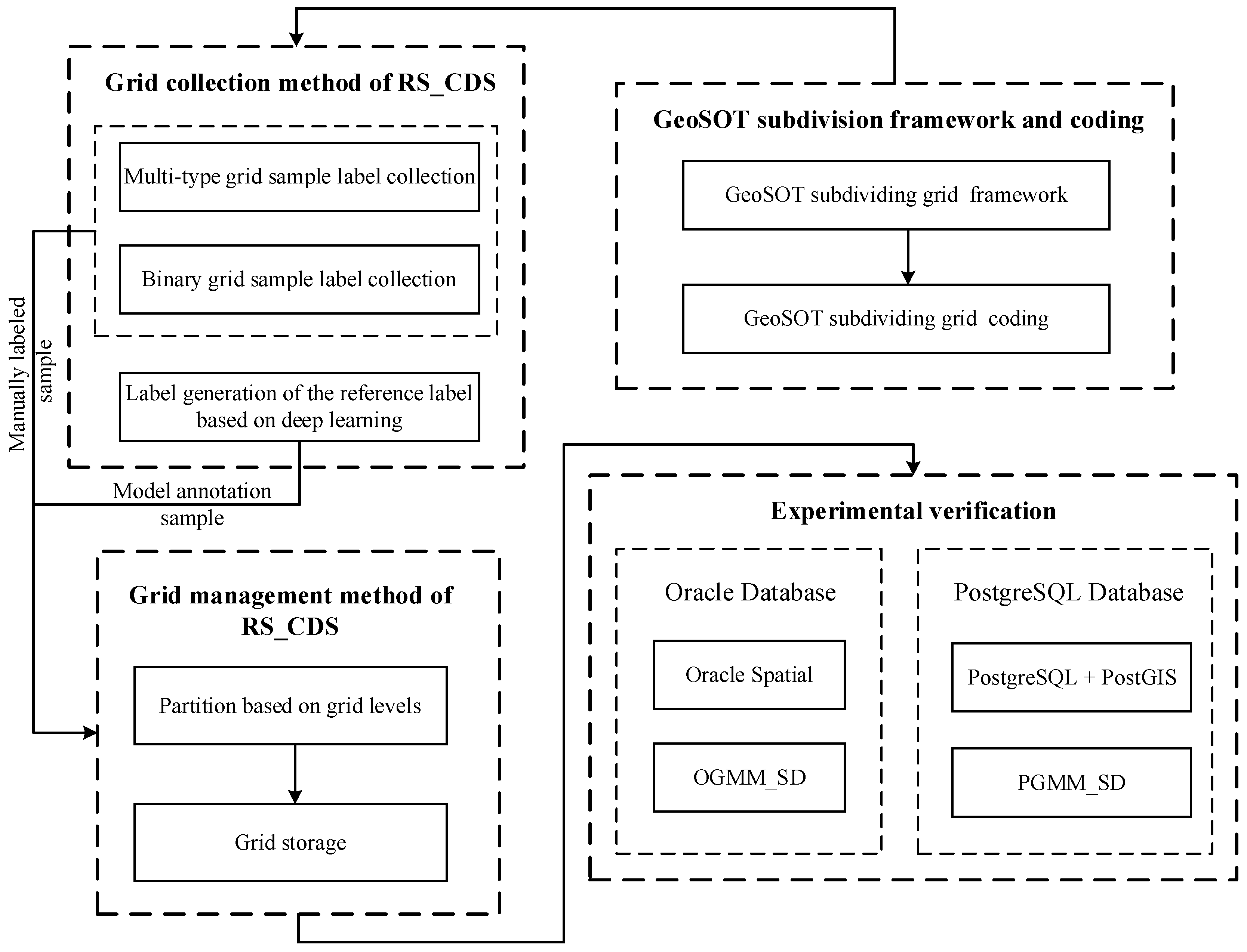
As shown in Figure 1, the RS_CDS were globally acquired using GCM-SD, signifying the annotation of the GeoSOT grid with attributes of ground objects or the types of changes within the grid. GCM-SD identifies the grid label using manual identification and model annotation. The global indexing and management of the RS_CDS were facilitated using GMM_SD. This paper proposes a grid collection and management model of RS_CDS based on GeoSOT (GCAM-GeoSOT) to realize the real-time and efficient sharing of samples and learning results, and provide support for the iteration of the grid deep learning model.
2. Materials and Methods
2.1. GeoSOT Subdivision Framework and Coding
The geographic coordinate subdividing grid with one-dimensional integer coding on a 2n-tree (GeoSOT) [22] is a grid space subdivision and coding method for the Earth’s surface. GeoSOT, as one of the methods of AA DGGS, discretizes the Earth’s surface into a group of multi-level geometric units with similar shapes and regular sizes, and identifies and expresses them according to the unified coding rules to build a grid reference framework for geospatial data organization. This method expands the longitude and latitude coordinates three times, that is, 360° × 180° of the Earth space is extended to 512° × 512°, 60′ of 1° is extended to 64′, and 60″ of 1′ is extended to 64″. The GeoSOT grid system is composed of 32-level spatial grids. For each level, a quartering structure is adopted to perform the quartering subdivision of the integer degree, integer minute, and integer second, so as to form a multi-scale full quadtree recursive spatial grid system from the Earth (level 0) to the centimeter (level 32) level.
The main advantages of GeoSOT are the global coverage, seamless and non-overlapping data, complete scale, and retrievable and locatable data. Moreover, GeoSOT is well inclusive of existing data organization frameworks such as surveying and mapping, meteorology, ocean, and national geographic grids. GeoSOT subdivision identifiers have the uniqueness of coding, spatial relevance, and high retrieval efficiency. RS_CDS can adopt grid division and coding at all GeoSOT levels, and GeoSOT coding is used for grid positioning and area association identification. The image resolution and interpretation criteria of the RS_CDS are used to determine the GeoSOT level.
2.2. Grid Collection Method of RS_CDS (GCM-SD)
The collection of RS_CDS marks the GeoSOT grid with the ground object attributes or change types contained in the grid. Each grid is a basic collection unit. The unmarked image is the remote sensing change detection grid image (RS_CDGI), the marked sample is the remote sensing change detection grid sample (RS_CDGS), and the sample format is (Image, Label), to conduct model training to realize the detection and analysis of spatial attributes. RS_ CDGS includes the manually labeled sample RS_CDGS0 (Section 2.2.1 and Section 2.2.2) and the model annotation sample RS_CDGS1 (Section 2.2.3).
Spatial topological relation is an indispensable feature for describing ground objects [23], which takes the ground objects in the collection area as a whole for sample collection. In this way, both the spectral, texture, and shape features of samples can be extracted, as well as the spatial topological relationship between sample ground objects in the collection area. The grid feature vector can be constructed by combining grid image features and neighborhood grid information. At the same time, the grid sample avoids the fine drawing and collection of the boundary contour of ground objects, significantly reducing the workload of sample data collection and labeling, and improving the labeling speed for sample data.
This method adopted GeoSOT binary two-dimensional coding, which codes the grid longitude and latitude separately. The specific assignment of the GeoSOT binary one-dimensional code is as follows:
where is the longitude coordinate value or latitude coordinate value of the grid positioning point and is the GeoSOT subdivision level.
According to GeoSOT binary one-dimensional coding, the GeoSOT binary two-dimensional grid coding and annotation of the RS_CDGS can be expressed as
where is the longitude coordinate value, is the latitude coordinate value, is the GeoSOT subdivision level, and label is the change detection type of the grid corresponding to the code at the subdivision level .
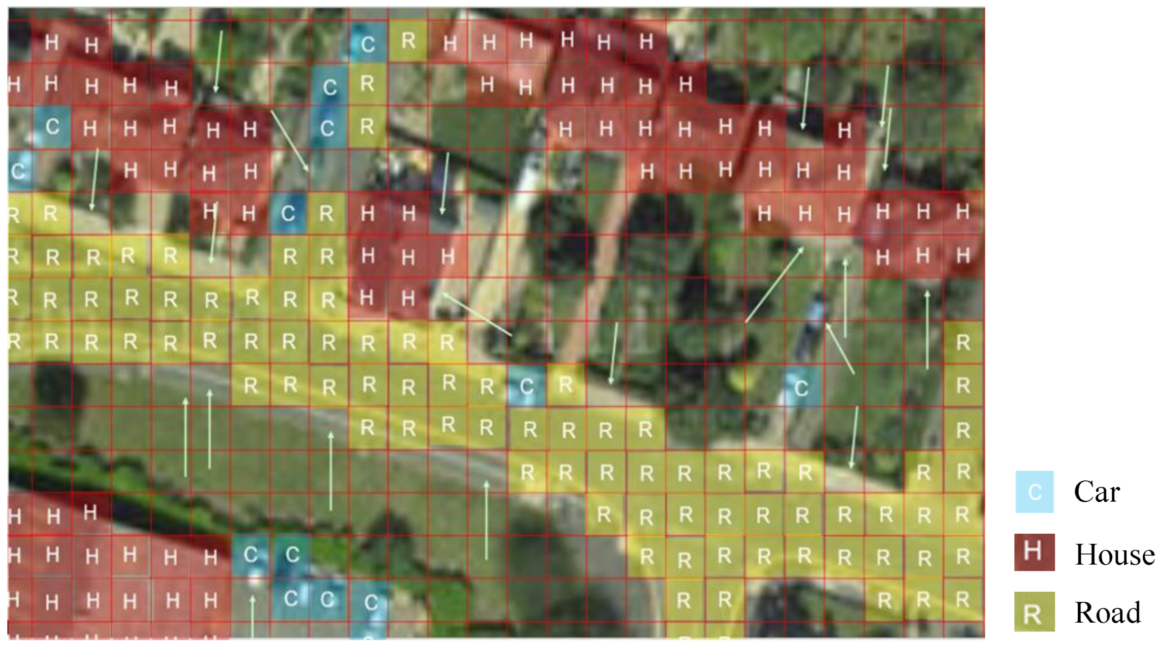
2.2.1. Multi-Type Grid Sample Label Collection
As shown in Figure 2, the collection of sample data is marked by taking the grid as the unit, which can be completed quickly by directly selecting the type of the ground object (i.e., car, house, or road) in the grid sample, and the corresponding label set is . However, when labeling samples using a grid as the unit, it is often impossible for a certain type of ground object to occupy a complete grid; in particular, the ground object may occupy only a small part of the grid, or the ground object may occur in the middle line of two adjacent grids, such as the grid indicated by the white arrow in Figure 2. This issue poses a significant challenge to the accuracy of sample data.
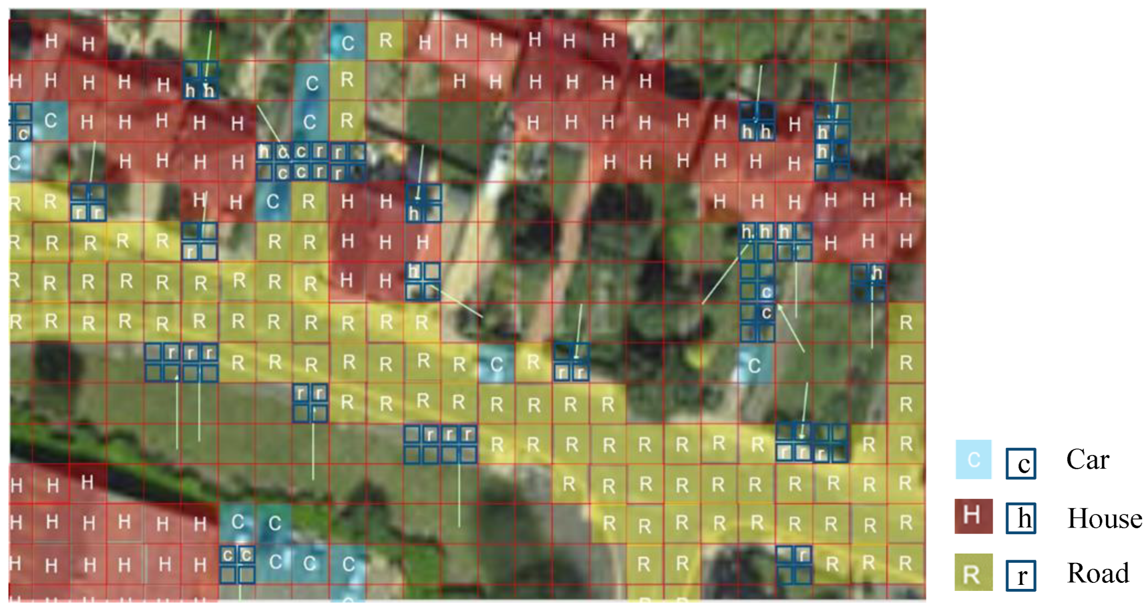
According to the theory of GeoSOT subdivision generation, the next level grid is a recursive quad subdivision of the previous level grid, so that the current level grid () at the edge of the ground object is divided into four, , and the next level grid is labeled to improve the precision of sample marking.
We add a judgment indicator and a judgment threshold for judging which edge area of the ground object needs to go to the next-level subdivision. is the proportion of the area of within the grid. The specific formula for is expressed as follows:
where is the area of within the grid and is the area of the grid. In this paper, we set . If , we do not need to perform a next-level subdivision for the grid. If , we need to advance to the next-level subdivision for the grid.
As shown in the Figure 3, the area covered by the blue box is the sample collection area. For the area in the left blue box that needs to be collected, Z-sequence collection is carried out from to . If needs further subdivision (), Z-sequence collection is carried out from to . In this regard, we used the next-level GeoSOT subdivision grid to label the sample data in the edge area of the ground object, as shown in Figure 4.
2.2.2. Binary Grid Sample Label Collection
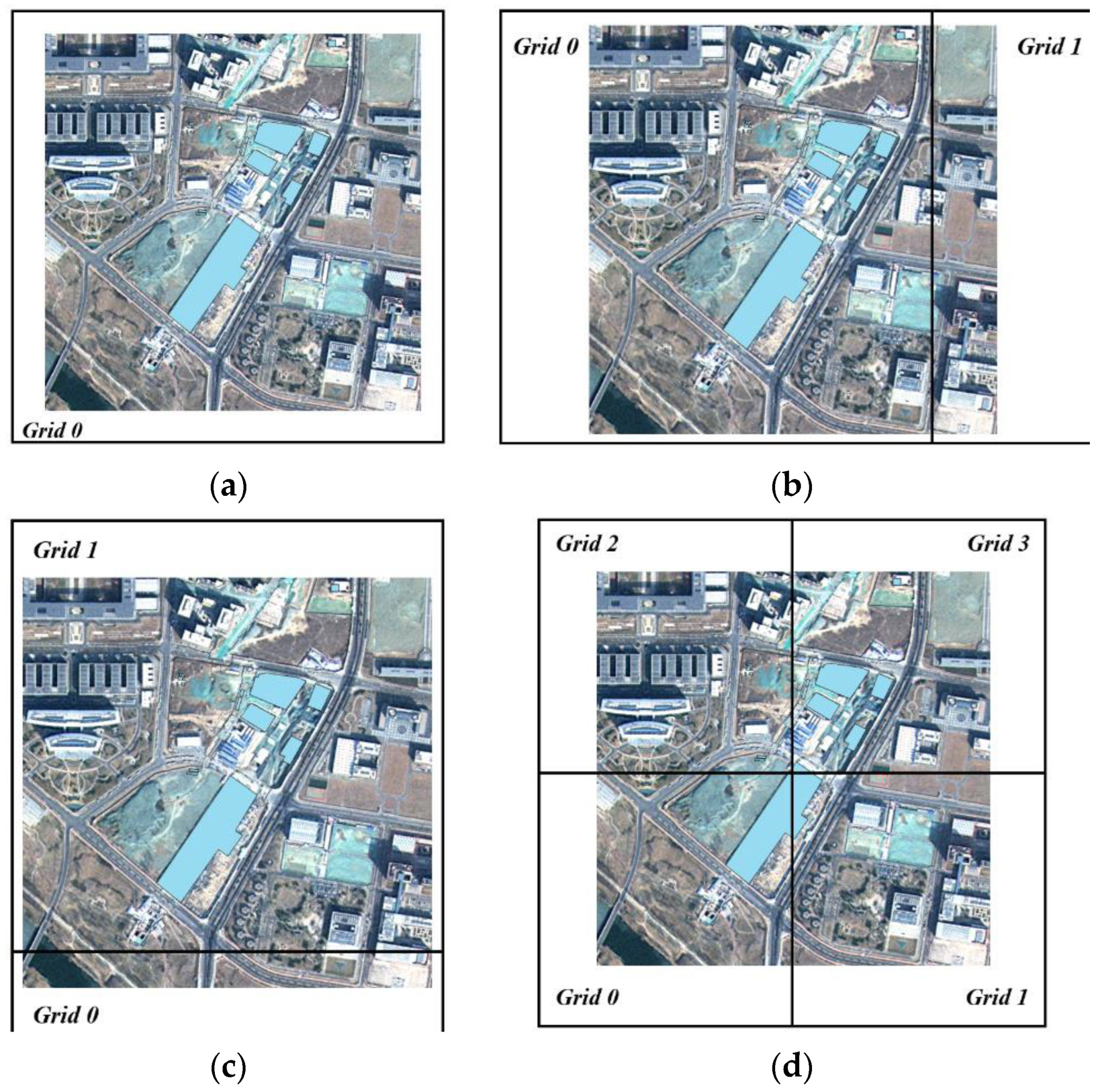
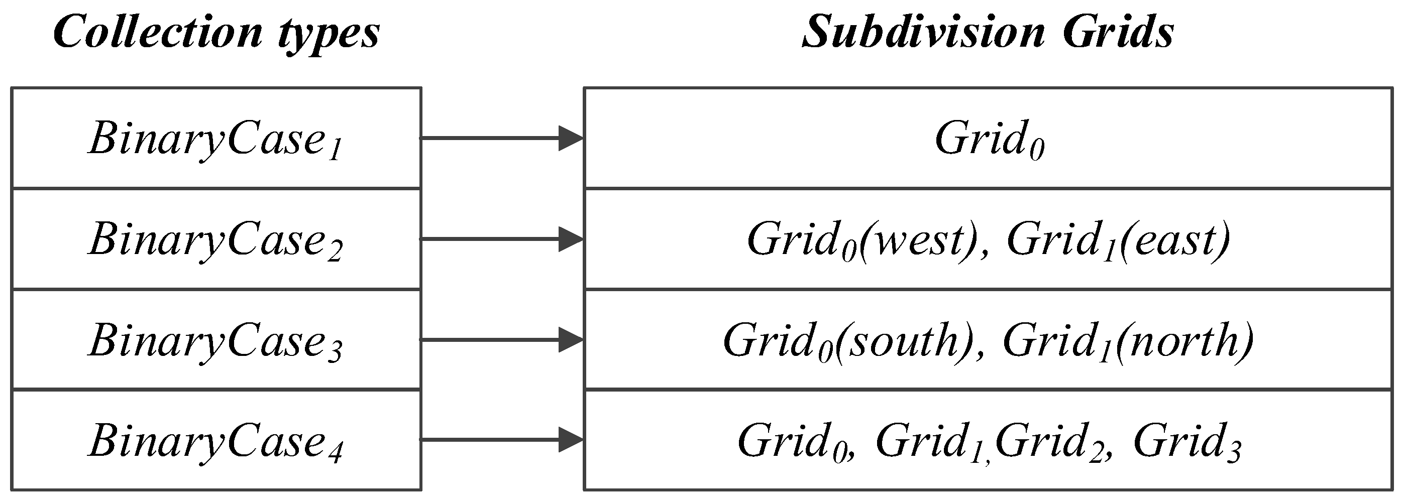
Binary (with or without change) RS_CDGS0 is the superposition of remote sensing images of different phases at the same location. The blue area in Figure 5 represents the change in the area. From left to right and from top to bottom, there are four grid collection types to generate binary RS_CDGS0, namely single-grid subdivision, east–west subdivision, north–south subdivision, and four-grid subdivision. The sample collection types and their corresponding sets of subdivision grids are shown in Figure 6.
2.2.3. Label Generation of Reference Label Based on Deep Learning
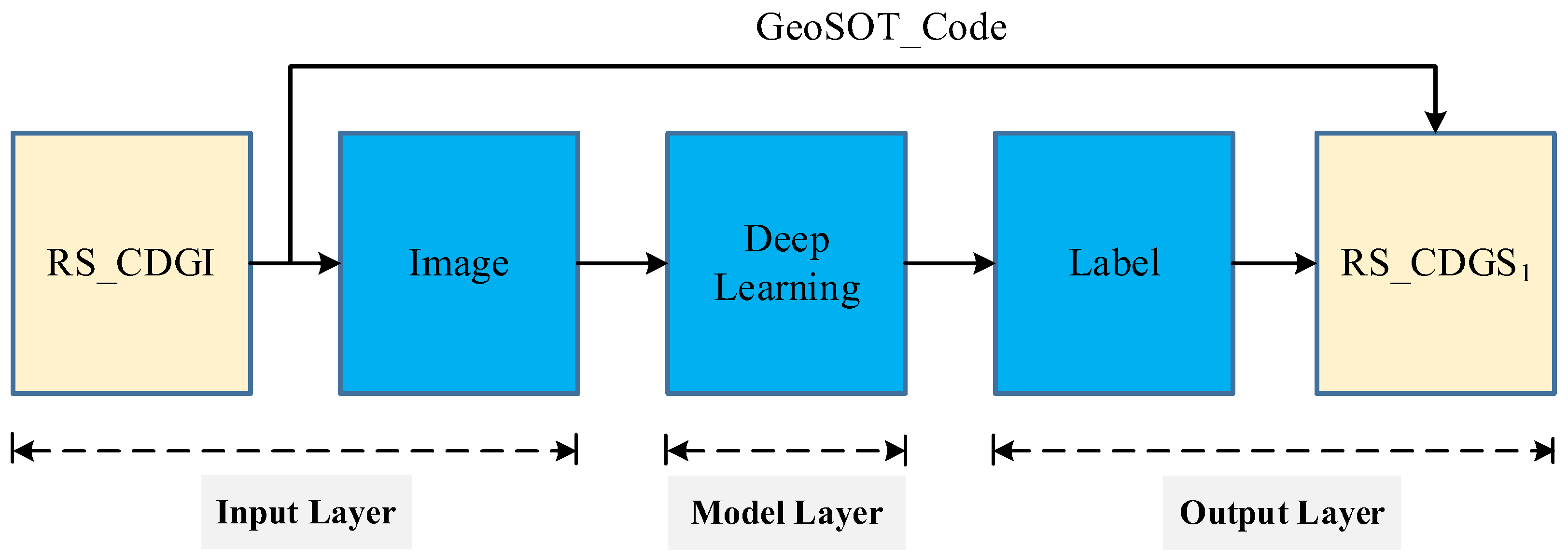
The remote sensing intelligent change detection of the RS_CDGS could define the grid level according to the requirements. Combined with deep learning, the RS_CDGS could automatically and efficiently obtain classification results and avoid the tedious manual interpretation and interpretation errors caused by the different scales of operators. The learning results of the deep learning model trained using RS_CDGS0 were used as the model iterative training grid samples. Based on the existing subdivision image, the label value was obtained using the deep learning model, and the RS_CDGI was automatically labeled as RS_CDGS1, which is a constructed complete grid sample used to provide sample data reference support for other model training in the same area, as shown in Figure 7.
2.3. Grid Management Method of RS_CDS (GMM-SD)
2.3.1. Partition Based on Grid Levels
GeoSOT grid coding provides data indexing support for the iteration of the grid deep learning model. The subdivision remote sensing samples in the same grid correspond to a unique coding ID, which realizes the query, statistics, and real-time sharing of samples and learning results. Moreover, GeoSOT binary extended coding can provide more efficient outputs based on its advantages of fast retrieval.
In this study, we established a two-level region partition mechanism for change detection via grid remote sensing (TRPM-GRSCD). The partitions were established as follow:
- GeoSOT grid first-level partition: establish grid subdivision units at the research area level and allocate the grid code ID of the research area under the research area subdivision level ). That is, establish multi-level grid storage units at the national, provincial, municipal, district, and street levels, and directly reach the samples based on to realize efficient retrieval. At the same time, the grid location expression avoids the ambiguity of multiple names in one location.
- GeoSOT grid second-level partition: establish a grid subdivision unit at the sample level, and allocate the sample grid code ID under the sample subdivision level .
2.3.2. Grid Storage
Via the GeoSOT spatial coding generation operation, the spatial location information of RS_CDGS is transformed into the GeoSOT subdivision code, and a large grid sample subdivision index table (LGSSIT) is established. The research area grid coding column and sample grid coding column based on GeoSOT associates the grid samples with spatial location information, which is used as the query primary key () to obtain the metadata of RS_CDGS. The specific formula for is expressed as follows:
where is the number of codes of the RS_CDGS under TRPM-GRSCD in the database, is the -th research area code under level , and is the -th sample code under level .
JavaScript Object Notation (JSON) is a lightweight data exchange format with good readability and extensibility, and has significant advantages in processing spatial data, such as the RS_ CDGS. In this study, we stored the JSON file and saved the association relationship between the GeoSOT code and grid samples to LGSSIT. RS_CDGS is located in the GeoSOT system according to its header file parameters. Then, we obtained the image of the RS_CDGS using the combination of the main path and sample name of the RS_CDGS, and retrieved of the RS_CDGS in the LGSSIT to obtain the complete RS_CDGS. The attribute storage expression formula of the LGSSIT is as follows:
where is the attribute information corresponding to , is the number of attribute columns, is the main path of the RS_CDGS, and is the defined attribute-containing operation.
3. Experiment
The purpose of the experiment conducted in this study was to verify the feasibility and retrieval efficiency of GMM_SD. This method combines the Oracle (OGMM_SD) and PostgreSQL (PGMM_SD) databases and compares the retrieval efficiency and database capacity with the corresponding spatial databases in Oracle Spatial and PostgreSQL + PostGIS. Oracle Spatial is a spatial data management system developed based on this feature of Oracle [24]. Oracle Spatial index establishment mainly includes MDSYS.SDO_GEOMETRY type field establishment and MDSYS.SPATIAL_INDEX type index establishment. PostGIS is a spatial extension of PostgreSQL, providing spatial information service functions such as spatial objects, spatial indexes, spatial operators, and spatial operation functions [25]. Oracle Spatial adopts an R-tree index and PostgreSQL + PostGIS adopts a GIST index.
The following formula was used to measure the retrieval efficiency improvement (), database capacity consumption (), and comprehensive performance () of GMM_SD:
where is the retrieval time of the comparative experiment, is the retrieval time of GMM_SD, is the database capacity consumption of GMM_SD, and is the database capacity consumption of the comparative experiment.
3.1. Experimental Data and Test Environment
The simulation generated approximately 15 million metadata of the RS_CDS as comparative experimental data, and the RS_CDGS formed by the GeoSOT subdivision was used as the experimental data. According to the image resolution of the simulated data, the 16th level of the GeoSOT grid was selected to manage the RS_CDS.
The experimental development platform used was Microsoft Visual Studio 2017, the programming language was C#, the CPU was Intel (R) Xeon (R) Gold 6132 @ 2.60 GHz 2.59 GHz (2 processor), and the memory was 64 GB. The backend database system was Oracle 11 g and PostgreSQL 9.6 + PostGIS 3.0.
3.2. Experiment and Analysis of Retrieval Efficiency
For the analysis of the retrieval efficiency, we arbitrarily selected different change detection research areas around the world, including custom triangular research areas, rectangular research areas, and polygonal research areas. Moreover, we retrieved the RS_CDS (RS_CDGS) in the research area, returned all attribute columns of the RS_CDS (RS_CDGS), and counted the number of returned RS_CDS (RS_CDGS). The comparison experiment time was the time required to return the retrieved RS_CDS, and the GMM_SD verification experiment time was the time required to retrieve the RS_CDGS using GeoSOT grid coding in the research area. To demonstrate the efficiency of the method proposed in this paper, the grid code ID of the research area was not provided in order to hinder the retrieval efficiency of the GMM_SD verification experiment and evaluate the retrieval advantage of GMM_SD.
The specific experimental research areas are listed in Table 1 and the GMM_SD code generation time (GGT) of the research area and the RS_CDGS number (NR) in the research area are shown in Table 2. Details of the specific areas are listed below:
- The triangular research area was defined as , where is longitude, is latitude, and is the span.
- The rectangular research area was defined as , where is longitude, is latitude, and is the span.
- The polygonal research area was defined as , where is longitude, is latitude, is span 1, and is span 2.
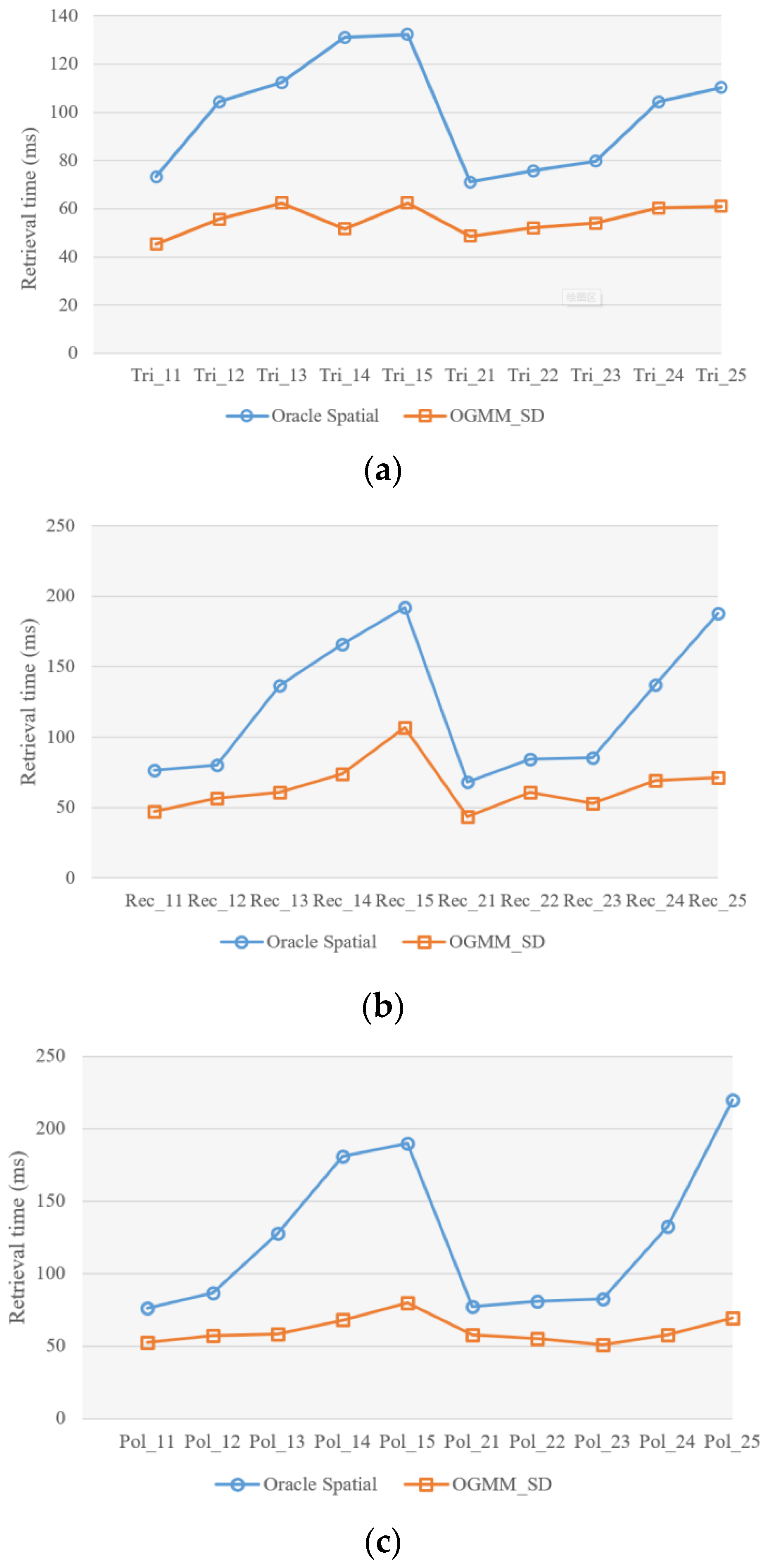
This study retrieved the RS_CDS (RS_CDGS) of the triangular research areas, rectangular research areas, and polygonal research areas. A comparison of the Oracle Spatial retrieval time and OGMM_SD retrieval time in the research areas is shown in Figure 8. The retrieval time was taken as the average of the three queries under the same conditions.
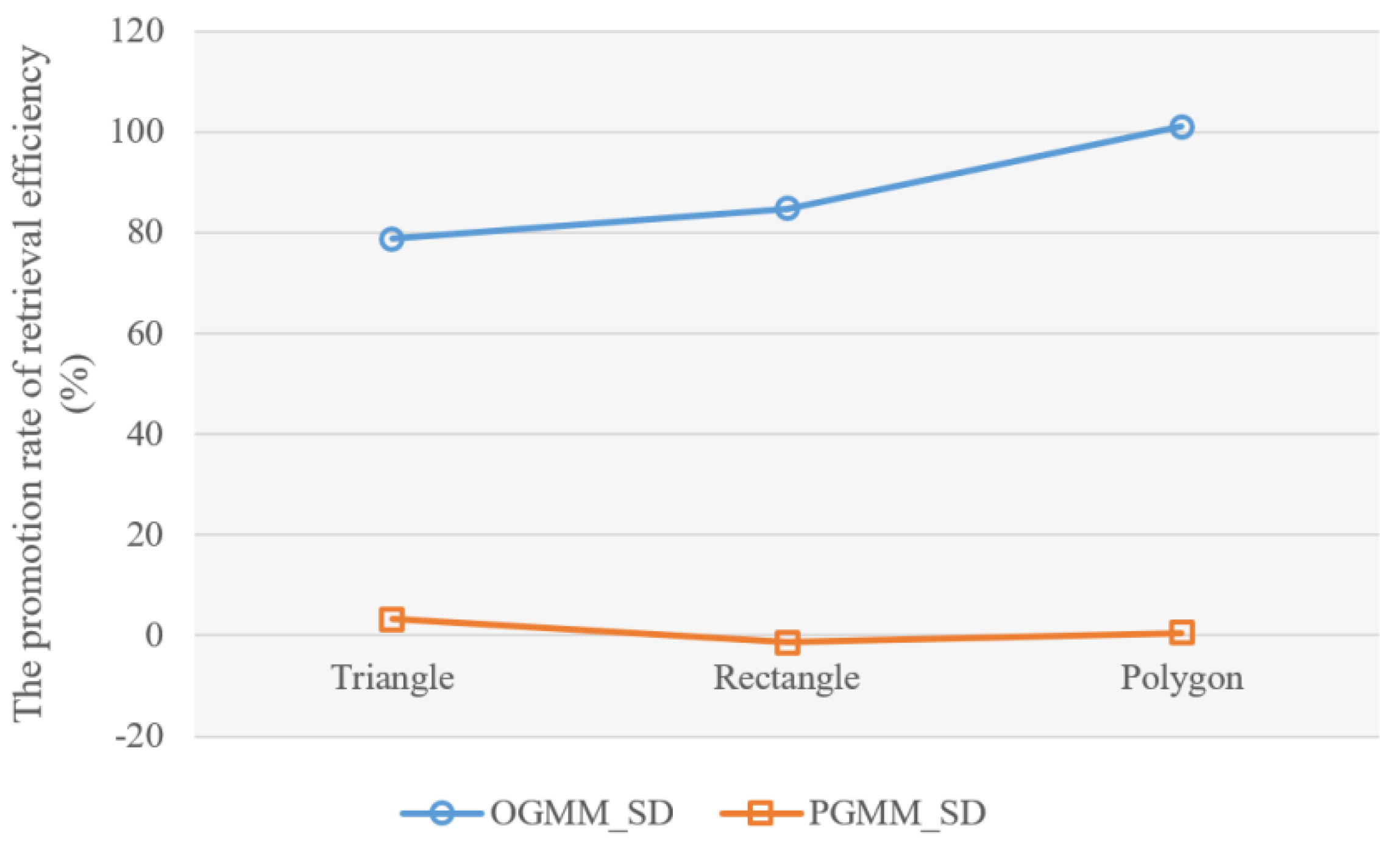
As can be seen from the above experiment, the retrieval experiment of the metadata of 15 million RS_CDS revealed that compared with Oracle Spatial, OGMM_SD had an average increase of 78.80% in the triangular research areas, 84.84% in the rectangular research areas, and 101.01% in the polygonal research areas, and the total average retrieval efficiency of RS_CDS was improved by 88.22%. The retrieval time of the RS_CDS was reduced by GeoSOT binary coding, resulting in a higher retrieval efficiency. Moreover, with an increase in the value, the larger the space of the research area, the lower the overall trend of the retrieval efficiency, indicating a negative correlation between the retrieval efficiency and size of the research area. For the triangular, rectangular, and polygonal research areas, showed an increasing trend, indicating a positive correlation between with increasing complexity of the research area.
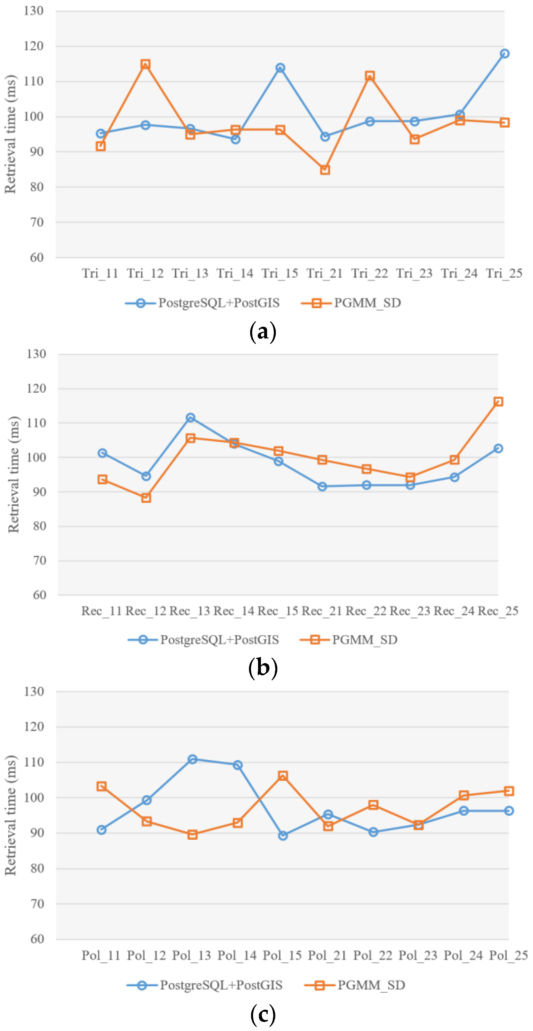
The comparison of the PostgreSQL + PostGIS retrieval time and PGMM_SD retrieval time in the research areas is shown in Figure 9. The retrieval time was taken as the average of the three queries under the same conditions.
As shown in Table 3 and Figure 10, PGMM_SD increased by 3.26% in the triangular research areas, decreased by 1.40% in the rectangular research areas, and increased by 0.58% in the polygonal research areas, and the total average for the RS_CDS was 0.81%. Moreover, the overall RS_CDS retrieval efficiency of PGMM_SD was slightly improved compared with that of PostgreSQL + PostGIS.
3.3. Database Capacity Comparison
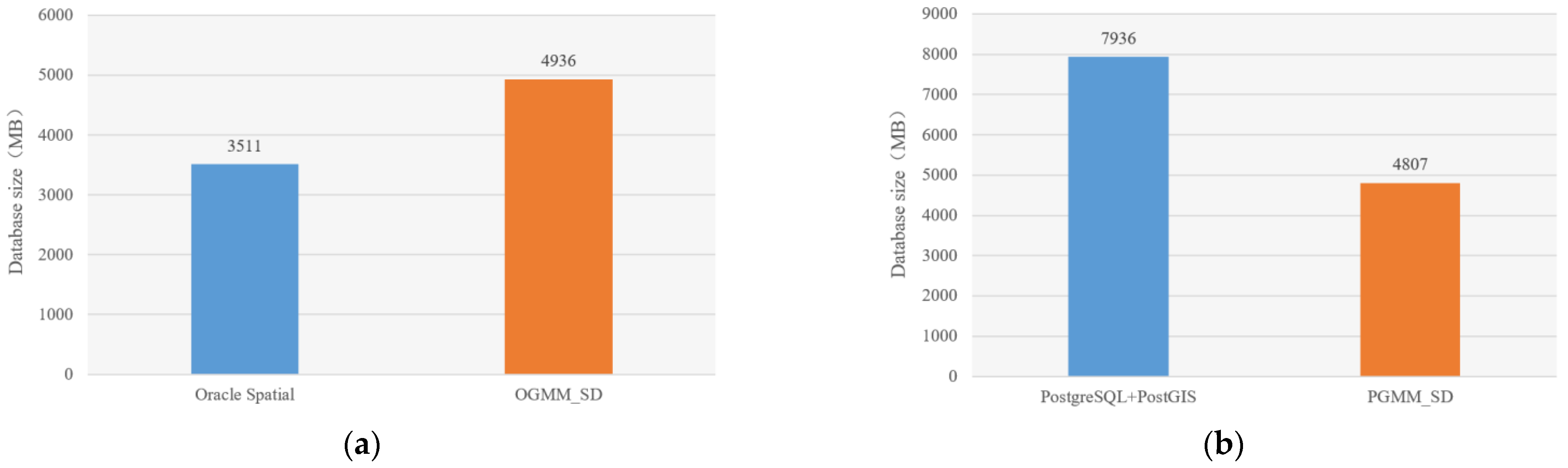
In the experiment, the comparison of the database capacity between Oracle Spatial and OGMM_SD is shown in Figure 11a. In the Oracle database, the of OGMM_SD was 40.59% when the retrieval efficiency of the RS_CDS was improved. As shown in Table 4, the of OGMM_SD was 47.63%, indicating that OGMM_SD performs better than Oracle Spatial in terms of time consumption and space consumption. A comparison of the database capacity between PostgreSQL + PostGIS and PGMM_SD is shown in Figure 11b. In the PostgreSQL + PostGIS database, the creation of the GIST index took a long time and occupied a large space. The of PGMM_SD was 39.43% when the retrieval efficiency of the RS_CDS was slightly improved, improving the storage cost. As shown in Table 4, the of PGMM_SD was 40.24%, indicating that PGMM_SD performed better than PostgreSQL + PostGIS in terms of time consumption and space consumption.
4. Conclusions
Compared with the local grid, GeoSOT unified grid coding is characterized by spatiotemporal uniqueness. Moreover, GeoSOT unified grid coding can automatically associate the RS_CDS of various types and resolutions as well as the attribute values corresponding to the RS_CDS with the spatial location of RS_CDS in any region of the world. In this study, GCAM-GeoSOT was constructed to associate the RS_CDS with the grid; that is, the RS_CDS were collected globally using GCM-SD, and globally indexed and managed using GMM_SD. Based on the results of our experiment, the following two conclusions were deduced: (1) GCM-SD identifies the grid label using manual identification (Section 2.2.1 and Section 2.2.2) or model annotation (Section 2.2.3) in order to rapidly collect and establish grid information labels. Grid information labels can be used for rapid target positioning, change monitoring, and regional statistics, which is convenient for location-based monitoring services and the collection of rapid statistics for a broad information range. It is also suitable for sensitive remote sensing application services for both the public and individuals. The samples and their learning results are accurately shared in real time, providing sample support for the iteration of the urban regional change intelligent monitoring model. (2) Compared with Oracle Spatial, the retrieval efficiency of OGMM_SD was improved by 88.22%, the database capacity of OGMM_SD was 40.59% higher, and the comprehensive performance of OGMM_SD was improved by 47.63%. Moreover, compared with PostgreSQL + PostGIS, the retrieval efficiency of PGMM_SD was improved by 0.81%, the database capacity consumption of PGMM_SD was reduced by 39.43%, and the comprehensive performance of PGMM_SD was improved by 40.24%. Overall, GMM_SD exhibited a more comprehensive performance in terms of the RS_CDS retrieval efficiency and database capacity consumption than Oracle Spatial.
This study only discussed the performance of GCAM-GeoSOT under the 16th level GeoSOT grid, which has general limitations. Future work will further explore the performance of the GCAM-GeoSOT at different scales and study the applicability of the model.
Author Contributions
Conceptualization, D.Z. and F.R.; data curation, D.Z.; formal analysis, D.Z.; funding acquisition, D.Z., M.H. and C.C.; investigation, D.Z. and F.R.; methodology, D.Z.; project administration, F.R.; resources, D.Z. and F.R.; software, D.Z.; supervision, E.A.S., F.R. and C.C.; validation, D.Z.; writing—original draft, D.Z.; writing—review and editing, B.H., S.L. and M.H. All authors have read and agreed to the published version of the manuscript.
Funding
This research was funded by the National Key Research and Development Programs of China, grant number 2018YFB0505300, the talent startup fund of Fuzhou University, grant number 511182, the National Nature Science Foundation of China (NSFC) program, grant number 42201438, and the Youth Program of Major Discipline Academic and Technical Leaders Training Program of Jiangxi Talents Supporting Project, grant number 20232BCJ23086.
Data Availability Statement
Restrictions apply to the availability of these data. The data are not publicly available due to privacy.
Acknowledgments
We appreciate the constructive suggestions and comments from the editor and anonymous reviewers.
Conflicts of Interest
The authors declare no conflict of interest.
References
- Akçay, H.G.; Aksoy, S. Building detection using directional spatial constraints. In Proceedings of the 2010 IEEE International Geoscience and Remote Sensing Symposium, Honolulu, HI, USA, 25–30 July 2010; pp. 1932–1935. [Google Scholar]
- Chen, J.; Lu, M.; Chen, X.; Chen, J.; Chen, L. A spectral gradient difference based approach for land cover change detection. ISPRS J. Photogram. Remote Sens. 2013, 85, 1–12. [Google Scholar] [CrossRef]
- Hulley, G.; Veraverbeke, S.; Hook, S. Thermal-based techniques for land cover change detection using a new dynamic modis multispectral emissivity product (mod21). Remote Sens. Environ. 2014, 140, 755–765. [Google Scholar] [CrossRef]
- Huang, M.; Chen, N.; Du, W.; Wen, M.; Zhu, D.; Gong, J. 2021. An on-demand scheme driven by the knowledge of geospatial distribution for large-scale high-resolution impervious surface mapping. GISci. Remote Sens. 2021, 58, 562–586. [Google Scholar] [CrossRef]
- Chen, Z.; Huang, M.; Zhu, D.; Altan, O. Integrating Remote Sensing and a Markov-FLUS Model to Simulate Future Land Use Changes in Hokkaido, Japan. Remote Sens. 2021, 13, 2621. [Google Scholar] [CrossRef]
- Shi, W.; Zhang, M.; Zhang, R.; Chen, S.; Zhan, Z. Change detection based on artificial intelligence: State-of-the-art and challenges. Remote Sens. 2020, 12, 1688. [Google Scholar] [CrossRef]
- Ma, L.; Liu, Y.; Zhang, X.; Ye, Y.; Yin, G.; Johnson, B.A. Deep learning in remote sensing applications: A meta-analysis and review. ISPRS J. Photogram. Remote Sens. 2019, 152, 166–177. [Google Scholar] [CrossRef]
- Maggiori, E.; Tarabalka, Y.; Charpiat, G.; Alliez, P. Can semantic labeling methods generalize to any city? The inria aerial image labeling benchmark. In Proceedings of the 2017 IEEE International Geoscience and Remote Sensing Symposium (IGARSS), Fort Worth, TX, USA, 23–28 July 2017. [Google Scholar]
- Xu, Y.; Du, B.; Zhang, L.; Cerra, D.; Pato, M.; Carmon, E.; Prasad, S.; Yokoya, N.; Hänsch, R.; Le Saux, B. Advanced multi-sensor optical remote sensing for urban land use and land cover classification: Outcome of the 2018 IEEE GRSS Data Fusion Contest. IEEE J. Select. Topic. Appl. Earth Obs. Remote Sens. 2018, 99, 1–16. [Google Scholar] [CrossRef]
- Hong, D.; Hu, J.; Yao, J.; Chanussot, J.; Zhu, X.X. Multimodal remote sensing benchmark datasets for land cover classification with a shared and specific feature learning model. ISPRS J. Photogram. Remote Sens. 2021, 178, 68–80. [Google Scholar] [CrossRef] [PubMed]
- Okujeni, A.; van der Linden, S.; Hostert, P. Berlin-Urban-Gradient Dataset 2009-an Enmap Preparatory Flight Campaign; EnMAP Consortium: Potsdam, Germany, 2016. [Google Scholar]
- Du, X.; Zare, A. Scene label ground truth map for MUUFL Gulfport Data Set. University of Florida: Gainesville, FL, Tech. Rep. 20170417. Available online: http://ufdc.ufl.edu/IR00009711/00001 (accessed on 13 March 2017).
- Goodchild, M.F. Reimagining the history of GIS. Ann. GIS 2018, 24, 1–8. [Google Scholar] [CrossRef]
- Purss, M.; Gibb, R.; Samavati, F.; Peterson, P.; Ben, J. The OGC® discrete global grid system core standard: A framework for rapid geospatial integration. In Proceedings of the 2016 IEEE International Geoscience and Remote Sensing Symposium (IGARSS), Beijing, China, 10–15 July 2016. [Google Scholar]
- Robertson, C.; Chaudhuri, C.; Hojati, M.; Roberts, S.A. An integrated environmental analytics system (IDEAS) based on a DGGS. ISPRS J. Photogram. Remote Sens. 2020, 162, 214–228. [Google Scholar] [CrossRef]
- Lin, B.; Zhou, L.; Xu, D.; Zhu, A.X.; Lu, G. A discrete global grid system for earth system modeling. Int. J. Geogr. Inf. Sci. 2017, 32, 711–737. [Google Scholar] [CrossRef]
- Gibb, R.G.; Purss, M.B.J.; Sabeur, Z.; Strobl, P.; Qu, T. Global reference grids for big Earth data. Big Earth Data 2022, 6, 251–255. [Google Scholar] [CrossRef]
- Gray, J.; Chaudhuri, S.; Bosworth, A.; Layman, A.; Reichart, D.; Venkatrao, M.; Pellow, F.; Pirahesh, H. Data Cube: A relational aggregation operator generalizing group-by, cross-tab, and sub-totals. Data Min. Knowl. Discov. 1997, 1, 29–53. [Google Scholar] [CrossRef]
- Rao, J.; Gao, S.; Li, M.; Huang, Q. A privacy-preserving framework for location recommendation using decentralized collaborative machine learning. Trans. GIS 2021, 25, 1153–1175. [Google Scholar] [CrossRef]
- Gu, T.; Feng, K.; Cong, G.; Long, C.; Wang, Z.; Wang, S. The RLR-Tree: A Reinforcement Learning Based R-Tree for Spatial Data. Proc. ACM Manag. Data 2023, 1, 1–26. [Google Scholar] [CrossRef]
- Viloria, A.; Acuña, G.C.; Franco, D.J.A.; Hernández-Palma, H.; Fuentes, J.P.; Rambal, E.P. Integration of data mining techniques to PostgreSQL database manager system. Procedia Comput. Sci. 2019, 155, 575–580. [Google Scholar] [CrossRef]
- Cheng, C.; Ren, F.; Puo, G.; Wang, H.; Chen, B. Introduction to Spatial Information Subdivision and Organization; Science Press: Beijing, China, 2012. (In Chinese) [Google Scholar]
- Shen, J.; Zhang, L.; Chen, M. Topological relations between spherical spatial regions with holes. Int. J. Digital Earth 2020, 13, 429–456. [Google Scholar] [CrossRef]
- Oracle. Oracle Spatial. 2023. Available online: https://docs.oracle.com/en/database/oracle/oracle-database/21/spatl (accessed on 1 September 2023).
- Meyer, T.; Brunn, A. 3D Point Clouds in PostgreSQL/PostGIS for Applications in GIS and Geodesy. GISTAM 2019, 1, 154–163. [Google Scholar]
Figure 1.
Overall structure of this study.

Figure 2.
Primary collection of multi-type grid samples.

Figure 3.
Grid collection of sample types based on Z-order encoding.

Figure 4.
Secondary collection of multi-type grid samples.

Figure 5.
The four collection types of binary grid samples. (a) Single-grid subdivision collection type. (b) East–west subdivision collection type. (c) North–south subdivision collection type. (d) Four-grid subdivision collection type.
Figure 5.
The four collection types of binary grid samples. (a) Single-grid subdivision collection type. (b) East–west subdivision collection type. (c) North–south subdivision collection type. (d) Four-grid subdivision collection type.

Figure 6.
Sample collection types and their corresponding sets of subdivision grids.

Figure 7.
Sample generation of the reference label based on deep learning.

Figure 8.
Comparison of the Oracle retrieval times: (a) comparison of the Oracle retrieval time in the triangular research areas; (b) comparison of the Oracle retrieval time in the rectangular research areas; and (c) comparison of the Oracle retrieval time in the polygonal research areas.
Figure 8.
Comparison of the Oracle retrieval times: (a) comparison of the Oracle retrieval time in the triangular research areas; (b) comparison of the Oracle retrieval time in the rectangular research areas; and (c) comparison of the Oracle retrieval time in the polygonal research areas.

Figure 9.
Comparison of PostgreSQL retrieval time: (a) comparison of PostgreSQL retrieval time in triangular research areas; (b) comparison of PostgreSQL retrieval time in rectangular research areas; (c) comparison of PostgreSQL retrieval time in polygonal research areas.
Figure 9.
Comparison of PostgreSQL retrieval time: (a) comparison of PostgreSQL retrieval time in triangular research areas; (b) comparison of PostgreSQL retrieval time in rectangular research areas; (c) comparison of PostgreSQL retrieval time in polygonal research areas.

Figure 10.
Average improvement of retrieval efficiency of OGMM_SD and PGMM_SD.

Figure 11.
Database capacity comparison: (a) comparison of database capacity between Oracle Spatial and OGMM_SD; and (b) comparison of database capacity between PostgreSQL + PostGIS and PGMM_SD.
Figure 11.
Database capacity comparison: (a) comparison of database capacity between Oracle Spatial and OGMM_SD; and (b) comparison of database capacity between PostgreSQL + PostGIS and PGMM_SD.


Table 1.
Details on the specific experimental research areas used in this study. (The units for , , , and are in degrees).
Table 1.
Details on the specific experimental research areas used in this study. (The units for , , , and are in degrees).
| ID | ID | ID | |||
|---|---|---|---|---|---|
| Tri_11 | (−140, −40, 0.05) | Rec_11 | (−140, −40, 0.05) | Pol_11 | (−140, −40, 0.05, 0.025) |
| Tri_12 | (−140, −40, 0.1) | Rec_12 | (−140, −40, 0.1) | Pol_12 | (−140, −40, 0.1, 0.05) |
| Tri_13 | (−140, −40, 0.15) | Rec_13 | (−140, −40, 0.15) | Pol_13 | (−140, −40, 0.15, 0.075) |
| Tri_14 | (−140, −40, 0.2) | Rec_14 | (−140, −40, 0.2) | Pol_14 | (−140, −40, 0.2, 0.1) |
| Tri_15 | (−140, −40, 0.25) | Rec_15 | (−140, −40, 0.25) | Pol_15 | (−140, −40, 0.25, 0.125) |
| Tri_21 | (120, 50, −0.05) | Rec_21 | (120, 50, −0.05) | Pol_21 | (120, 50, −0.05, −0.025) |
| Tri_22 | (120, 50, −0.1) | Rec_22 | (120, 50, −0.1) | Pol_22 | (120, 50, −0.1, −0.05) |
| Tri_23 | (120, 50, −0.15) | Rec_23 | (120, 50, −0.15) | Pol_23 | (120, 50, −0.15, −0.075) |
| Tri_24 | (120, 50, −0.2) | Rec_24 | (120, 50, −0.2) | Pol_24 | (120, 50, −0.2, −0.1) |
| Tri_25 | (120, 50, −0.25) | Rec_25 | (120, 50, −0.25) | Pol_25 | (120, 50, −0.25, −0.125) |
Table 2.
GGT of the research area and NR in the research area.
| ID | GGT (ms) | NR | ID | GGT (ms) | NR | ID | GGT (ms) | NR |
|---|---|---|---|---|---|---|---|---|
| Tri_11 | 13.9847 | 22 | Rec_11 | 79.0057 | 42 | Pol_11 | 59.9723 | 38 |
| Tri_12 | 128.1201 | 80 | Rec_12 | 342.9543 | 144 | Pol_12 | 238.2658 | 115 |
| Tri_13 | 286.7505 | 177 | Rec_13 | 553.8344 | 342 | Pol_13 | 630.2579 | 276 |
| Tri_14 | 548.0029 | 304 | Rec_14 | 1154.6569 | 576 | Pol_14 | 828.2052 | 454 |
| Tri_15 | 864.2238 | 474 | Rec_15 | 1634.0458 | 900 | Pol_15 | 1480.9624 | 708 |
| Tri_21 | 25.3898 | 21 | Rec_21 | 48.4677 | 36 | Pol_21 | 15.2665 | 30 |
| Tri_22 | 155.1059 | 79 | Rec_22 | 323.4874 | 144 | Pol_22 | 199.3939 | 114 |
| Tri_23 | 311.2913 | 173 | Rec_23 | 684.4581 | 324 | Pol_23 | 453.3619 | 254 |
| Tri_24 | 633.2543 | 302 | Rec_24 | 1268.4975 | 576 | Pol_24 | 744.8747 | 452 |
| Tri_25 | 757.6348 | 467 | Rec_25 | 1528.6376 | 900 | Pol_25 | 1251.8714 | 708 |
Table 3.
Improvement of retrieval efficiency of OGMM_SD and PGMM_SD.
| Triangular Research Areas | Rectangular Research Areas | Polygonal Research Areas | Total Average | |
|---|---|---|---|---|
| OGMM_SD (%) | 78.80 | 84.84 | 101.01 | 88.22 |
| PGMM_SD (%) | 3.26 | −1.40 | 0.58 | 0.81 |
Table 4.
Storage consumption and comprehensive performance of OGMM_SD and PGMM_SD.
| Database Types | OGMM_SD | PGMM_SD |
|---|---|---|
| 40.59 | −39.43 | |
| 47.63 | 40.24 |
Disclaimer/Publisher’s Note: The statements, opinions and data contained in all publications are solely those of the individual author(s) and contributor(s) and not of MDPI and/or the editor(s). MDPI and/or the editor(s) disclaim responsibility for any injury to people or property resulting from any ideas, methods, instructions or products referred to in the content. |
© 2023 by the authors. Licensee MDPI, Basel, Switzerland. This article is an open access article distributed under the terms and conditions of the Creative Commons Attribution (CC BY) license (https://creativecommons.org/licenses/by/4.0/).
Share and Cite
MDPI and ACS Style
Zhu, D.; Han, B.; Silva, E.A.; Li, S.; Huang, M.; Ren, F.; Cheng, C. Novel Grid Collection and Management Model of Remote Sensing Change Detection Samples. Remote Sens. 2023, 15, 5528. https://doi.org/10.3390/rs15235528
AMA Style
Zhu D, Han B, Silva EA, Li S, Huang M, Ren F, Cheng C. Novel Grid Collection and Management Model of Remote Sensing Change Detection Samples. Remote Sensing. 2023; 15(23):5528. https://doi.org/10.3390/rs15235528
Chicago/Turabian StyleZhu, Daoye, Bing Han, Elisabete A. Silva, Shuang Li, Min Huang, Fuhu Ren, and Chengqi Cheng. 2023. "Novel Grid Collection and Management Model of Remote Sensing Change Detection Samples" Remote Sensing 15, no. 23: 5528. https://doi.org/10.3390/rs15235528
Note that from the first issue of 2016, this journal uses article numbers instead of page numbers. See further details here.