
Infrared Small-Target Detection Based on Background-Suppression Proximal Gradient and GPU Acceleration

1
National Key Laboratory of Optical Field Manipulation Science and Technology, Chinese Academy of Sciences, Chengdu 610209, China
2
Institute of Optics and Electronics, Chinese Academy of Sciences, Chengdu 610209, China
3
School of Electronic, Electrical and Communication Engineering, University of Chinese Academy of Sciences, Beijing 101408, China
*
Author to whom correspondence should be addressed.
Remote Sens. 2023, 15(22), 5424; https://doi.org/10.3390/rs15225424
Submission received: 1 October 2023
/
Revised: 5 November 2023
/
Accepted: 15 November 2023
/
Published: 20 November 2023
(This article belongs to the Special Issue Remote Sensing of Target Object Detection and Identification II)
Abstract
:Patch-based methods improve the performance of infrared small target detection, transforming the detection problem into a Low-Rank Sparse Decomposition (LRSD) problem. However, two challenges hinder the success of these methods: (1) The interference from strong edges of the
background, and (2) the time-consuming nature of solving the model. To tackle these two challenges,
we propose a novel infrared small-target detection method using a Background-Suppression
Proximal Gradient (BSPG) and GPU parallelism. We first propose a new continuation strategy to
suppress the strong edges. This strategy enables the model to simultaneously consider heterogeneous
components while dealing with low-rank backgrounds. Then, the Approximate Partial Singular
Value Decomposition (APSVD) is presented to accelerate solution of the LRSD problem and further
improve the solution accuracy. Finally, we implement our method on GPU using multi-threaded
parallelism, in order to further enhance the computational efficiency of the model. The experimental
results demonstrate that our method out-performs existing advanced methods, in terms of detection
accuracy and execution time.
1. Introduction
Infrared Small-Target Detection (ISTD) is an important component of infrared search and tracking, aiming to exploit the thermal radiation difference between a target and its background to achieve long-range target detection. According to the definition by the Society of Photo-Optical Instrumentation Engineers (SPIE), small targets typically refers to objects in a 256 × 256 image with an area of fewer than 80 pixels, accounting for approximately 0.12% of the total image area [1]. These small targets usually appear as faint, tiny points, characterized by their diminutive size and a lack of clear texture and shape features. Moreover, the background in infrared images is often affected by random noise, clutter, and environmental factors, making small targets vulnerable to interference. Furthermore, some practical applications have strict requirements on the real-time performance of detection algorithms. Therefore, the rapid and accurate detection of small targets in complex backgrounds poses a significant challenge.
Two primary methods are employed in ISTD for target detection: Tracking-Before-Detection (TBD) and Detection-Before-Tracking (DBT). TBD relies on the temporal information of consecutive frames to capture the movement and features of potential targets. It struggles with stationary or sporadically moving targets and is constrained by computational resources. On the other hand, DBT applies single-frame ISTD to infrared data, identifying potential targets based on features such as contrast and low-rank sparsity. Single-frame infrared small target detection has been widely concerned because of its simple data acquisition, low computational complexity, not affected by target motion, and wide applicability.
The categorization of single-frame ISTD can be determined by the structure of the image; that is, whether (1) the original image or (2) the patch image is used [2]. The first category detects the target directly from the original image; for example, by filtering or Human Vision System (HVS). Filter-based methods [3,4,5,6] have limited utility in ISTD, due to their strict requirements on the background variation and prior knowledge. Meanwhile, HVS-based methods [7,8,9,10,11] use the contrast mechanism to quantify the difference between the target and the background, thereby enhancing small targets. However, these methods are limited by the local saliency of the target, rendering them ineffective when detecting targets that are dark or similar to the background. Some deep learning technologies [12,13,14,15] have recently been applied to this category, but a lack of large data sets limits their performance.
The other category—namely, patch-based methods—transforms small target detection into a low-rank matrix recovery problem [16]. This transformation can circumvent the aforementioned limitations, such as the dependence on prior knowledge and target saliency, as well as the false detection of dark targets. The most popular method is Infrared Patch-Image (IPI) [17], which uses a sliding window technique to generate a corresponding patch image from the original image. Due to its outstanding performance, many studies [18,19,20,21,22,23,24,25,26] have been conducted on IPI, which typically yields superior results. However, patch-based methods still have two problems: (1) The misclassification of strong edges as sparse target components, and (2) the time-consuming nature of the method.
The above-mentioned misclassification arises from the limited ability of the model to distinguish strong edges from sparse components. To address this issue, we propose a Background Suppression Proximal Gradient (BSPG) method, incorporating a novel continuation strategy during the alternating updating of low-rank and sparse components. Our proposed continuation strategy can preserve more components while updating the low-rank matrix, while also reducing the update rate of sparse matrix. As strong edges frequently correspond to larger singular values than targets, the former facilitates the transition of strong edges from sparse components to low-rank components, thereby enabling the model to eliminate the affect of strong edges. Meanwhile, the latter ensures the convergence of the algorithm.
The time-consuming nature of patch-based methods is due to the complex nature of solving the method, mainly including solving the LRSD problem and constructing/reconstructing patch images. To address this issue, we utilize both algorithmic optimizations and hardware enhancements. At the algorithmic level, we propose an approximate partial SVD (APSVD) for efficiently solving the LRSD problem and use a rank estimation method to ensure the accuracy of the solution. At the hardware level, we propose the use of GPU multi-threaded parallelism strategies to expedite the construction and reconstruction modules, as these modules can be decomposed into repetitive and independent sub-tasks.
Our main contributions can be summarized as follows:
- A novel continuation strategy based on the Proximal Gradient (PG) algorithm is introduced to suppress strong edges. This continuation strategy preserves heterogeneous backgrounds as low-rank components, hence reducing false alarms.
- The APSVD is proposed for solving the LRSD problem, which is more efficient than the original SVD. Subsequently, parallel strategies are presented to accelerate the construction and reconstruction of patch images. These designs can reduce the computation time at the algorithmic and hardware levels, facilitating rapid and accurate solution.
- Implementation of the proposed method on GPU is executed and experimentally validate its effectiveness with respect to the detection accuracy and computation time. The obtained results demonstrate that the proposed method out-performs nine state-of-the-art methods.
The remainder of this paper is organized as follows: Section 2 presents the related work. Section 3 details our proposed BSPG algorithm and GPU acceleration strategies. Section 4 introduces the data set and experimental settings, as well as providing the experimental results and analysis. Section 5 discusses the results of the experiments. Section 6 gives a summary of our method.
2. Related Work
2.1. HVS-Based Methods
HVS-based methods detect small targets by utilizing the contrast differences between the target region and its surrounding background. These methods can be categorized based on the type of information they use: grey scale information, gradient information, and a combination of both grey scale and gradient information. Local Contrast Measure (LCM) [1] proposes a novel method for detecting small targets by leveraging grey scale contrast. This method uses a contrast mechanism designed to enhance small targets while effectively suppressing the background noise. Based on the improvement of LCM algorithm, Relative Local Contrast Measure (RLCM) [8], Multiscale Patch-based Contrast Measure (MPCM) [9], Weighted Local Difference Measure (WLDM) [27] and other methods were proposed. Gradient-based contrast methods use first-order or second-order derivatives of the image to extract gradient information. They then utilize this information to design a gradient difference measure that effectively discriminates between small targets and the surrounding background. Building on this concept, Derivative Entropy-based Contrast Measure (DECM) [28] and Local Contrast-Weighted Multidirectional Derivative (LCWMD) [29] propose the use of multidirectional derivative to incorporate more gradient information. In addition, Local Intensity and Gradient (LIG) [30], Gradient-Intensity Joint Saliency Measure (GISM) [31] fuse gradient and intensity information to further highlight small targets. Although HVS-based methods can be effective in many scenarios, they are susceptible to missed detections and false positives in images characterized by low signal-to-clutter ratios and high-intensity backgrounds.
2.2. Deep Learning-Based Methods
In recent years, there has been a significant research focus on deep learning-based methods for infrared small target detection, which seek to achieve high-accuracy detection rates. These deep learning models are trained to discern features within infrared images using vast datasets, thereby enhancing their detection capabilities. To address the problem that infrared small target features are easily lost in deep neural networks, Attention Local Contrast Network (ALCNet) [32] proposes asymmetric contextual modulation to interact the feature information between the high and low levels. Dense Nested Attention Network (DNANet) [15] adequately fuses feature information through densely nested interaction modules to maintain small targets in deep layers. Miss Detection vs. False Alarm (MDvsFA) [33] proposes dual generative adversarial network models, trained inversely to decompose the detection challenge into sub-problems, aiming to strike a balance between miss detections and false alarms. While publicly available datasets have advanced deep learning for infrared small target detection, the scant features of small targets and the dependency on training samples limit the applicability of the model in varied real-world scenarios.
2.3. Patch-Based Methods
A significant amount of research has been conducted to improve the detection ability of IPI [17]. On one hand, some methods have used prior constraints, including Column-Weighted IPI (WIPI) [18], Non-negative IPI with Partial Sum (NIPPS) [20], and Re-Weighted IPI (ReWIPI) [21]. On the other hand, some studies have identified limitations in the nuclear norm and L1 norm and, so, alternative norms to achieve improved target representation and background suppression have been proposed; for example, Non-convex Rank Approximation Minimization (NRAM) [22] and Non-convex Optimization with Lp norm Constraint (NOLC) [23] introduce non-convex matrix rank approximation coupled with L2,1 norm and Lp norm regularization, while Total Variation Weighted Low-Rank (TVWLR) [24], Kernel Robust Principal Component Analysis (KRPCA) [25] introduce total variation regularization, High Local Variance (HLV) [26] method present LV* norm to constrain the background’s local variance. Patch-based methods mainly consider the low-rank nature of the background, affecting their performance in the presence of strong edges. However, our method pays additional attention to heterogeneous background suppression in low-rank constraints, in order to avoid this problem.
2.4. Acceleration Strategies for Patch-Based Methods
Acceleration strategies for patch-based methods can be categorized into algorithm-level and hardware-level acceleration. The first category mainly relies on the strategy of reducing the number of iterations. Self-Regularized Weighted Sparse (SRWS) [34] and NOLC [23] improve the iteration termination condition for acceleration, but still suffer from the time consumption associated to decomposing large matrices. The other category (i.e., hardware acceleration) relies on the use of computationally powerful hardware and efficient parallelization strategies. In [35], the researchers proposed Separable Convolutional Templates (SCT); however, this method has poor performance under complex backgrounds. In addition, extending the patch model to tensor space can also achieve acceleration [36,37,38,39,40,41]. Representative methods in this direction include Re-weighted Infrared Patch-Tensor (RIPT) [36], LogTFNN [39] and the Pareto Frontier Algorithm (PFA) [37]. However, unfolding the tensor into a two-dimensional matrix before decomposition increases the algorithm’s complexity. Partial Sum of the Tensor Nuclear Norm (PSTNN) [38] and Self-Adaptive and Non-Local Patch-Tensor Model (ANLPT) [42] utilize the t-SVD speed up tensor decomposition with t-SVD. However, these methods are limited by the complexity of finding the applicable constrained kernel norm. Our work investigates accelerated patch-based methods at both the algorithmic and hardware levels.
3. Method
In this section, we present the details and principles of the proposed method. First, a novel continuous strategy is proposed for the suppression of strong edges. Then, APSVD is used to accelerate solution of the LRSD problem. Finally, the integration of our proposed method on GPU is presented. The overall framework is shown in Figure 1.
3.1. BSPG Model
The infrared image is considered to be composed of the target image, background image, and noise image, formulated as
where , , , and represent the original infrared, background, target, and noise images, respectively. The IPI model uses a sliding window (from top-left to bottom-right) to convert the original image into a patch image. The IPI model can be formulated as
where D, B, T, and N represent the patch image, background patch image, target patch image, and noise patch image, respectively. Then, we can transform the small-target detection problem into the following convex optimization under broad conditions; that is,
where represents the nuclear norm, represents the column sum norm, is a positive weighting parameter, and . This convex optimization problem is called robust principle component analysis (RPCA), which can recover low-rank and sparse parts of the data matrix even when a fraction of the entries are missing. Let , , where is a relaxation parameter. Hence, we can express Equation (3) as
The PG algorithm is an efficient method to solve the RPCA problem, which estimates the background image and the target image by minimizing the separable quadratic approximation sequence of Equation (4); that is,
where , is the Lipschitz constant (which is set to 2 in this problem), and is a given parameter. The following function has a unique optimal solution as Equation (5) is convex:
where . In our method, Equation (5) can be expressed as:
To solve Equation (6), the iterative process of the PG algorithm repeatedly sets , and is obtained from . In our method, to be solved are ordered pairs . Therefore, we set
where is the sequence satisfying .
The closed-form expression of can be obtained by soft-thresholding the singular values. The soft-threshold operation is defined as
Then,
where is the SVD of .
The continuation strategy in [43] can speed up the convergence of the PG. This technique employs a decreasing sequence to derive , where is updated as follows:
The value of affects the convergence of the algorithm. A larger decrease results in more components to be retained, while fewer iterations to update results in an inability to separate the target. Conversely, a smaller decrease has the opposite effect. Figure 2 shows examples of the target images at different iterations. It can be seen that, in the early iterations, the strong edges are separated first as the low component of the background is retained at the highlights. This leads to many false alarms at the strong edges when the target is separated. This phenomenon motivates us to use different decrement rates for and . We set a higher rate for and set to compute more singular values, in order to retain strong edges. We also set a lower rate for , ensuring that the target is decomposed into sparse parts when the algorithm converges. Thus, is updated as follows:
where . The solution of the BSPG algorithm is described in Algorithm 1.
The upper bound of the algorithm is discussed below. By denoting as the sequence obtained by the algorithm with , according to [44], for any , we have
Then,
when , where the convergence accuracy is , yielding that the algorithm has iteration complexity.
| Algorithm 1: BSPG solution via APSVD |
 |
3.2. APSVD
The most time-consuming step in each iteration of the PG algorithm is the execution of the full SVD. It is worth mentioning that the soft-threshold operation only leaves a portion of the singular values and vectors to participate in the subsequent calculations. In particular, few singular values are needed in early iterations. Therefore, it is feasible to replace full SVD with partial SVD. The crucial step of this strategy is rank estimation, which involves estimating the number of singular values and singular vectors participating in the computation after truncation. As the noise in infrared images is often not simply Gaussian distributed, estimation functions such as minimax estimator or the simple quantitative increase method proposed in [43] are not feasible. Due to the low-rank nature of the patch image, the singular value matrix has a clear trend of change, as shown in Figure 3. Thus, we estimate the rank by evaluating the degree of variation of the singular values. In the kth iteration, the pre-determined rank is initialized by the number of singular values in S greater than . We update as follows:
where is the threshold for measuring the degree of singular value variation, N is the width of the patch image, and and are empirically set to 0.95 and 0.1, respectively.
The truncated SVD of the patch image needs to satisfy two requirements: (1) Only a small number of large singular values are retained, and (2) the singular vectors (including the left and right) need to be computed. We approximate the SVD of the patch image A by solving the eigenvalue decomposition of its covariance matrix . Given the slender nature of the patch matrix, the latter computation is considerably more straightforward compared to the former. Moreover, the symmetry of guarantees its suitability for eigenvalue decomposition, leading to
It is apparent, from Equation (16), that the eigenvalues of correspond to the squares of the singular values of A. Additionally, both the right singular vectors of A and the eigenvectors of are unitary. This relationship further implies that the left singular vectors U follow the equation . The approximate SVD of matrix A satisfies
where depends on the rounding errors. The singular values and singular vectors of the eigendecomposition in CUDA can approximate the accuracy of SVD to machine zero [45]. Furthermore, the larger the singular value, the smaller the error of U.
3.3. GPU Parallel Implementation
The GPU implementation consists of three main parts: Constructing the patch image, solving the LRSD problem, and reconstructing the patch image. Our method uses GPU for implementation purposes, and CPU only for data transfer and GPU control.
3.3.1. Construction
In order to reduce the number of data transfers between the host memory and the device’s global memory, we first copy all the image data and hyperparameters read by the CPU to the GPU via PCI Express, and then execute the parallelization kernel functions. GPU parallelism mainly relies on data parallelism, i.e., performing the same operation on multiple data elements. Correspondingly, a patch image is constructed to change the storage location of each pixel in the original image. Therefore we build an index mapping between the original image and the patch image. This mapping allows a thread to manage the correspondence of a pixel position, facilitating the parallel processing of all pixels.
Let , denote the width and height of the sliding window, , denote the sliding step in the x, y directions, and p denotes the number of patches in the x direction. The mapping of the patch image pixel index to the original image pixel index is
The execution of the kernel function requires the determination of the thread block and grid size, where the grid size is determined based on the number of processing subtasks and the thread block size. Suppose the output image size n of the kernel function is and the thread block size k is set to (where , denote the size of the image in the x and y direction, respectively, and , denote the number of threads per block in the x and y direction, respectively), then the grid size is determined as , where operator is defined as
We set the thread block size for the construction kernel function based on the size of the patch image. Assuming that the patch image dimensions are , we configure the thread block size as . For instance, given an image with a size of , a sliding window with a size of , and a sliding step of 10, the size of the resulting patch image would be . Accordingly, the thread block size is set to and the grid dimensions are set to . Consequently, a row of threads in the x direction corresponds to a row within the patch image. The construction process is carried out pixel-by-pixel. The processing time of each pixel is assumed to be t, for an patch image, serial execution of the construction module takes . In contrast, our method operates threads in parallel, completing the process in time t. The theoretical speedup ratio is .
3.3.2. Reconstruction
Figure 4 shows the steps for reconstructing the background and target patch images after LRSD. First, the target patch image is transformed into the pre-filtered image. We provide the pseudo-code for this transformation in Algorithm 2. Then, the indices of the first and last patches containing valid information are determined. Finally, filtering is performed on the valid portions of each row to obtain the target image. In summary, the reconstruction includes two parallel processes: One involving mapping from the patch image to the pre-filter image, and another entailing filtering.
| Algorithm 2: The mapping of patch image and pre-filter image |
| Input: Patch image D, original image size w and h, patch size and , step s, patch number of per row Output: pre-filter image F
|
We set the thread block and grid of the mapping kernel to the same size as the construction kernel. The filter kernel handles a much larger matrix, and in order to improve the resource usage, the thread block size is set to , and the grid size is obtained according to Equation (19). Then, the indices of the first patch and the last patch , containing valid information can be expressed as:
In NVIDIA’s GPU architecture, one warp typically consists of 32 threads, while our thread block contains threads. This means that each warp can effectively execute an entire thread block. This high warp occupancy rate reaches 100%, efficiently harnessing the performance of the GPU.
3.3.3. APSVD Using CUDA
The key to implementing the APSVD is the exact eigendecomposition, which can be achieved using the Symmetric Eigenvalue Divide (SYEVD) function based on QR decomposition or the Symmetric Eigenvalue Jacobi (SYEVJ) function based on Jacobi decomposition [46]. SYEVD employs a divide-and-conquer method to decompose a symmetric matrix into smaller sub-problems and solves them recursively. Its runtime is primarily attributed to QR decomposition. QR decomposition can be expressed as
where Q is an orthogonal matrix and R is an upper triangular matrix. QR decomposition usually requires Householder transformations for multiple iterations, and each transformation needs to manipulate all elements of the matrix, which becomes redundant for small matrices.
SYEVJ transforms the symmetric matrix A into a diagonal matrix D by performing a rotational transformation via the bilateral Jacobi method.
where J is denoted as , contains the rotation angle and an index pair , and satisfies . The Jacobi method, with its element-wise rotations, offers lower computational complexity, localized memory access, and parallelization potential, making it more efficient for small matrices.
To quantitatively analyze both methods, we introduce arithmetic intensity [46] which is a metric used to evaluate the performance of parallel computational tasks. Specifically, the arithmetic intensity I is defined as
where FLOPs represents the number of floating point operations and can measure the complexity of an algorithm, bytes loaded represents the number of bytes loaded from memory during kernel execution. Given an matrix (single-precision), a Givens rotation typically requires 8 floating-point operations (2 trigonometric functions, 4 multiplications, 2 additions) and loads elements. This means that the number of FLOPS per iteration is 8, and the memory access requires loading bytes. In QR decomposition, the computational complexity of each iteration, which involves Householder transformations, is , and it loads the entire matrix, including bytes. The arithmetic intensity of the Jacobi kernel and the arithmetic intensity of the QR decomposition kernel can be expressed as
Therefore, from the perspective of arithmetic intensity, we choose the more efficient Jacobi method to perform eigenvalue decomposition. The Jacobi method typically has lower arithmetic intensity and is relatively memory-access efficient, whereas QR decomposition involves orthogonal transformations and matrix updates, often requiring more memory bandwidth and computation. QR decomposition has a higher arithmetic intensity, making it perform better on larger matrices where the high arithmetic intensity can be fully utilized, but not on small matrices.
Furthermore, the implementation of APSVD requires an efficient matrix multiplication function. The General Element-wise Matrix Multiply (GEMM) function in CUDA takes advantage of the GPU’s parallel computing capabilities and efficiently processes substantial amounts of data, thereby enhancing computational performance. To reduce routing errors, we use the double precision-controlled GEMM function, DGEMM, which has a time complexity of . Notably, other functions utilize single precision to strike a balance between instruction throughput and accuracy. Figure 5 illustrates the runtime ratios for each component of APSVD on matrices of varying size. Notably, the efficiency of SYEVJ is demonstrated, as it is unaffected by the matrix height and exhibits a decreasing ratio of time spent on eigendecomposition as the matrix size increases.
4. Experiments and Analysis
In this section, we provide an evaluation of our method in terms of detection accuracy and execution time.
4.1. Experimental Setup
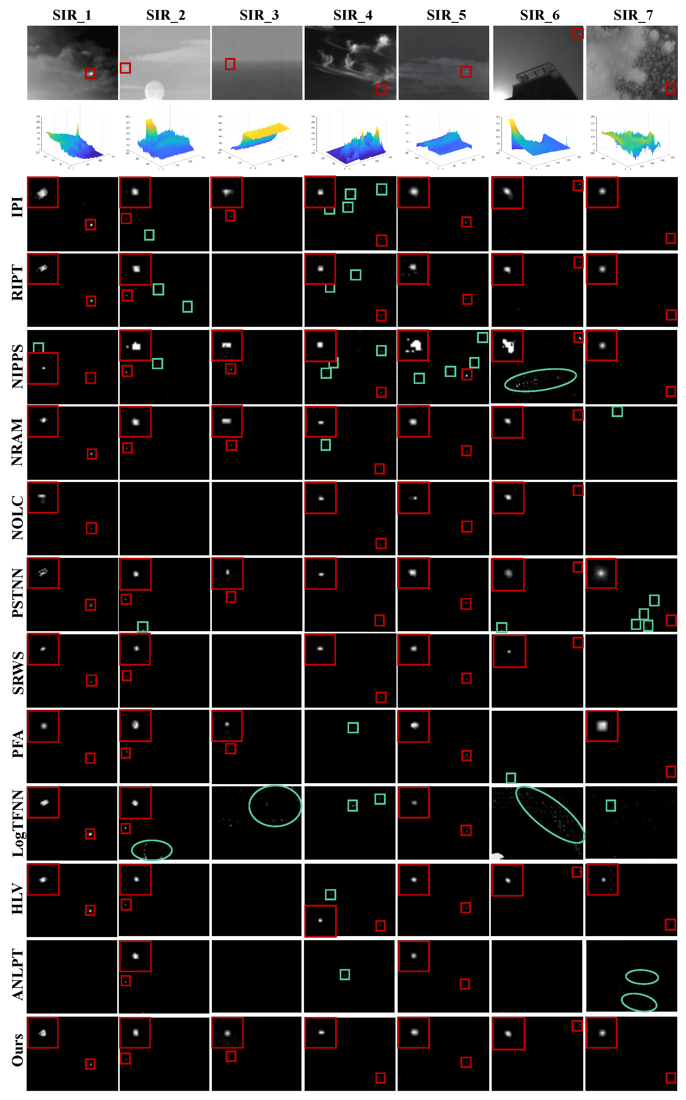
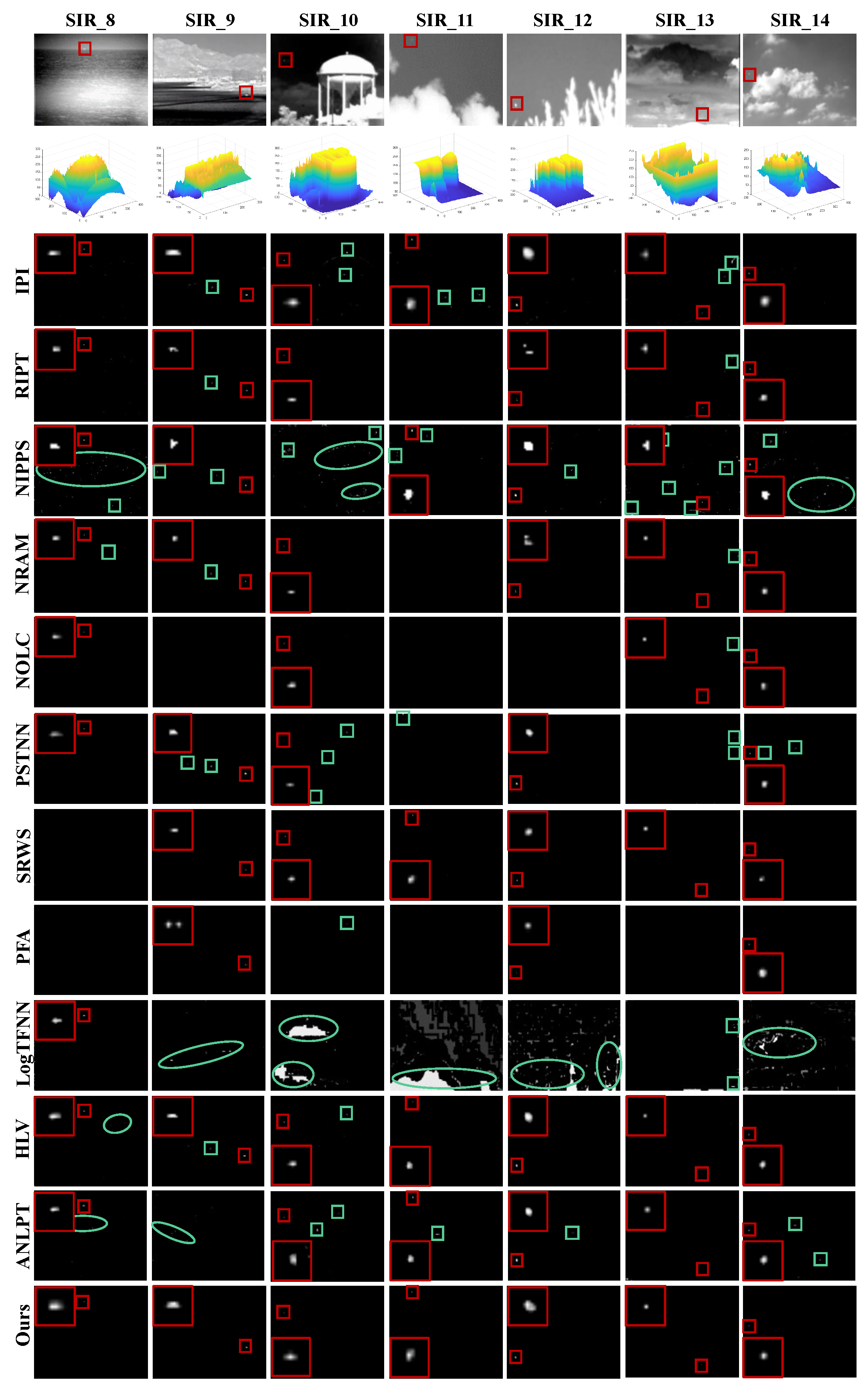
Data. The experiments used the real single-frame infrared images provided in [32], selected from infrared sequences in a variety of scenes, including ocean, cloud, sky, and urban areas, as shown in Figure 6. The targets are marked with red boxes and magnified for convenient viewing in the bottom left corner of each image. It can be seen that the targets occupy very few pixels; most small targets lack shape and texture information and have low intensity. Images with poor imaging quality exhibit strong noise, such as SIR_2 and SIR_3. Some small targets are submerged in cloud or sea clutter as SIR_11 and SIR_13 and suffered from highlight backgrounds with strong edges as SIR_8 to SIR_14. Furthermore, we provide detailed information of the test images, including the background type, target type, Signal Clutter Ratio (SCR), target size, and detection challenges, in Table 1.
Hardware. We implemented our method on the embedded GPU Jetson AGX Xavier, which has 7764 MB of global memory and 48 KB of shared memory. The version of CUDA was 10.2. The experiments in MATLAB were based on an Intel(R) Core(TM) i7-8750H CPU with 8 GB RAM.
Baselines and parameter settings. We compared our proposed method to other state-of-the-art patch-based methods, including IPI [17], NIPPS [20], NRAM [22], NOLC [23], SRWS [34] and HLV [26]. As tensor-based methods have better performance in terms of computational efficiency, we also included three tensor-based methods for comparison, including RIPT [36], PSTNN [38], PFA [37], LogTFNN [39] and ANLPT [42]. The parameter settings are provided in Table 2. We employed a sliding window with a size of and a step size of 30 on images with resolution equal to or exceeding . This setting ensured that the execution time remained within the desired range.
Evaluation metrics. We used two quantitative analysis evaluation indicators commonly used for small-target detection to evaluate our method: Signal Clutter Ratio Gain (SCRG) and Background Suppress Factor (BSF). SCRG reflects the effect of increasing target saliency, and is defined as follows:
where and represent the signal-to-clutter ratio of the input and output images, respectively, represents the average pixel gray value of the target, represents the average pixel gray value of the local background around the target, and represents the standard deviation of the gray pixel value of the local background around the target. BSF reflects the effect of suppressing background interference and is defined as follows:
where and are the standard deviation values of the local background around the target in the output image and the original image, respectively.
We also analyzed the results using Receiver Operating Characteristic (ROC) curves. The ROC curve is plotted by assessing the True Positive Rate (TPR) and the False Positive Rate (FPR) at different classification thresholds, as defined below:
To quantitatively compare the ROC curves, the area under the curve (AUC) can be used as an evaluation criterion; the larger the AUC, the more accurate the detection performance.
4.2. Visual Comparison with Baselines
The visualization results of twelve detection methods are shown in Figure 7 and Figure 8. IPI, RIPT, and NIPPS only successfully detect targets under simple backgrounds with high local patch similarity. In images with complex backgrounds, NIPPS present noticeable clutter, while IPI and RIPT exhibit noise in highlighted backgrounds. NRAM and PFA can detect the majority of targets, but they are prone to generating false alarms in regions with strong edges. NOLC and SRWS suffer from the sea surface background and can not detect weak dark targets. PSTNN has similar poor performance, with many false alarms under clutter. LogTFNN is poorly detected under high-intensity backgrounds, leaving a large amount of background residue. HLV and ANLPT perform poorly when detecting targets that are dark or have low contrast with the neighboring background. In the case of images SIR_7 to SIR_14, the highlighted backgrounds cause most methods to produce false alarms near strong edges, leading to inaccurate detection. However, our method excels in terms of effectively suppressing strong edges under such conditions. From the visualized detection results, our method exhibits robust detection performance.
4.3. Quantitative Evaluation and Analysis
The results of the quantitative comparison of the various methods on the test images are shown in Table 3. From the definitions of the two evaluation metrics, the larger the SCRG and BSF values, the better the detection results. In terms of BSF, our method performs better than the other methods on all images, indicating that our method excels in suppressing the background. In terms of SCRG, our method outperforms the other methods on most images. When the target is missed, the local background standard deviation is 0. Consequently, this leads to the SCRG appearing as a NaN result and BSF tending to infinity. In addition, we plotted the ROC curves corresponding to the experiments, in order to further validate the effectiveness of our method. The results in Figure 9 demonstrate that our method outperforms the other comparative methods on the test images. IPI and NIPPS are sensitive to clutter and high-intensity backgrounds due to the difficulty in distinguishing between targets and strong edges. NRAM and NOLC exhibit instability in detecting dim and weak targets. HLV experiences an increase in false alarms when dealing with strong clutter interference on the sea surface. Tensor-based detection methods show stable performance in simple backgrounds. However, RIPT and LogTFNN exhibit low detection accuracy in high-intensity backgrounds due to their high requirements for sparsity. PSTNN and PFA tend to erroneously reject targets in the presence of background clutter. SRWS demonstrates effective clutter suppression in high-intensity backgrounds but struggles to detect low-contrast weak targets. ANLPT exhibits weaker clutter suppression capabilities in high-intensity structured backgrounds. In contrast, our method achieves remarkable results in terms of detection accuracy and false alarm rate in a wide range of scenarios.
To evaluate the execution speed of our method, we compared our method with other patch-based methods. For fair comparison, we set these methods to share the same patch and step configurations. We implemented our method in two versions; that is, CPU and GPU versions. The GPU execution time includes the data transfer time between the host and the device. To ensure the reliability of the time statistics, we took the average time of 10 executions for each method. The comparison results are presented in Table 4. Most patch-based methods are time-consuming due to iteration and complex matrix decomposition, including IPI, NIPPS, and NRAM. RIPT and ANLPT relatively improve the detection efficiency, but the tensor decomposition is still complex. SRWS and HLV optimise the iterative termination conditions to achieve a faster detection speed. The results demonstrate that our method achieved impressive speed, particularly with significant acceleration when using the GPU. Combined with the previous detection accuracy evaluation, our method was found to achieve faster detection while maintaining higher accuracy.
4.4. Ablation Study
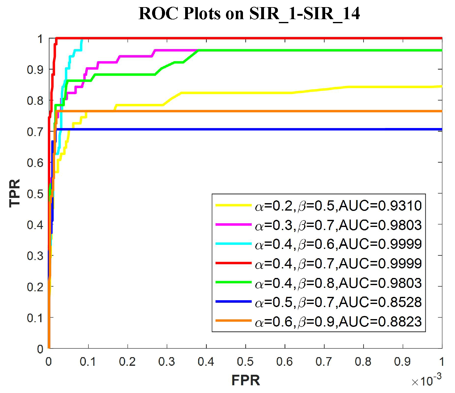
The effect of relaxation parameters. We explored the effects of the relaxation parameters and on the detection accuracy of our method using ROC curves. Figure 10 shows that excessively large or small values of and led to a decrease in the AUC value. Small can retain more background components, but overly small values result in insufficient iteration, thereby failing to separate targets. Meanwhile, large and values can cause false alarms by decomposing strong edges into sparse target portions. Therefore, we set and to 0.4 and 0.7, respectively.
Comparison with other tensor-based methods. For a fair comparison, we studied the tensor-based methods under the same settings as used for ours. We evaluated their detection accuracy and execution time under various patch and step configurations. Table 5 shows the execution time results. When using the same patch and step settings, our method on GPU is faster than PFA, PSTNN, and LogTFNN. As illustrated in Figure 11, our method consistently achieves the best detection accuracy across most scenarios. However, the detection accuracy of PFA, PSTNN, and LogTFNN significantly diminishes between images with variations in the patch size and step values.
The acceleration effect of different strategies. To validate the speed enhancement due to our proposed APSVD, we compared its implementations on both MATLAB 2017b and CUDA 10.2 platforms with various SVD functions, as shown in Table 6. It can be observed that APSVD exhibits high efficiency on slender matrices. To explore the effectiveness of the proposed acceleration strategies, we conducted tests on their cumulative acceleration effects over the baseline method IPI. Table 7 demonstrates that our proposed acceleration strategies yield commendable speed increases. Notably, PASVD avoids the intricate decomposition of large matrices, thus significantly saving time; the new continuation strategy employs a greater decrement for the relaxation parameters, reducing the number of iterations and consequently accelerating the overall speed; and the GPU parallel strategies provide significant acceleration, especially for larger images.
The acceleration effects on images with different attributes. To validate the acceleration effect of the proposed method, we conducted experiments on images with varying attributes (i.e., resolution and background complexity). As shown in Figure 12, the acceleration effect of our method becomes more pronounced with increasing image resolution. On an image with a resolution of , the execution speed of the proposed method is nearly 60 times faster than that of IPI. Due to the influence of image complexity on execution time, the acceleration effect varies slightly at the same resolution. Furthermore, we conducted a comparative analysis of the three stages of our method—namely, constructing a patch image, solving the LRSD problem, and reconstructing a patch image—as shown in Figure 13. It is evident that multi-threading parallelism and optimized memory access significantly reduce the time required for the construction and reconstruction modules. Additionally, the new continuation strategy and APSVD greatly contribute to reducing the time required to solve the LRSD problem.
5. Discussion
Patch-based methods are well-studied in single-frame infrared small target detection for their reliability. The classical IPI algorithm is a notable example. It transforms the original image into a patch image and leverages the non-local self-similarity of the background to enhance the low-rank property of the patch image. This method allows for effective infrared small target detection through low-rank and sparse decomposition.
In our comparison of small target detection methods, we observed that methods like NIPPS, NRAM, and NOLC aim to improve detection accuracy by enhancing the nuclear norm and l1 norm. However, these methods involve complex matrix decomposition and iterative processes, leading to time-consuming issues. These methods also struggle to differentiate between the edges and the actual targets due to the local sparsity of strong edges. Conversely, SRWS and HLV, with their proposed multi-subspace assumptions and high local variance constraints, generally perform well in most cases. They effectively suppress strong edges but may miss dark and weak targets. Additionally, these methods require complex matrix decomposition, making them time-consuming. RIPT expands the patch model into tensor space, adding to the computational burden as tensors are unfolded and decomposed. While tensor-based methods such as PSTNN, PFA, and logTFNN have accelerated detection somewhat, their effectiveness is limited by the challenges of accurately approximating nuclear norms within tensor models.
This paper aims to strike a balance between detection performance and time consumption. To address interference from strong edges, the BSPG method proposed in this paper introduces a novel continuous strategy in the alternating update process of low-rank and sparse components. This allows the model to mitigate the influence of strong edges by preserving more components while updating the low-rank matrix. For algorithm acceleration, a combined approach involving algorithm optimization and hardware enhancement is presented. On the algorithmic front, APSVD is introduced to expedite solving the LRSD problem. On the hardware front, we suggest utilizing GPU multi-thread parallel strategies to accelerate the construction and reconstruction of modules. This is possible as these modules can be decomposed into repetitive and independent subtasks. Visual and quantitative results from experiments demonstrate that our method outperforms other state-of-the-art methods. However, there is still room for improvement in terms of time performance, and in the future, we plan to explore even faster methods.
6. Conclusions
In this paper, we proposed a novel infrared small-target detection method using background-suppression proximal gradient and GPU parallelism. Considering that patch-based methods often result in false alarms at strong edges, we first proposed a novel continuation strategy to suppress such background interference. Then, we presented APSVD to accelerate the solution of the LRSD problem, which involves complex and time-consuming large matrix decomposition. Moreover, we employed GPU multi-threading parallelism to accelerate the construction and reconstruction of patch images. Finally, we optimized the proposed method on the GPU, ultimately achieving outstanding performance. The obtained experimental results demonstrated that our method out-performs nine state-of-the-art methods in terms of both detection accuracy and computational efficiency. The proposed GPU parallelism strategy can be applied to infrared motion sensors and other patch-based infrared small-target detection methods, thus facilitating their application in practical engineering.
Author Contributions
Conceptualization, X.H.; data curation, X.H.; investigation, T.L.; methodology, X.H.; software, X.H. and Y.L.; writing—original draft, X.H.; writing—review & editing, X.L. and Y.C. All authors have read and agreed to the published version of the manuscript.
Funding
This work was funded by the CAS “Light of West China” Program.
Data Availability Statement
The data presented in this study are cited within the article.
Conflicts of Interest
The authors declare no conflict of interest.
References
- Chen, C.P.; Li, H.; Wei, Y.; Xia, T.; Tang, Y.Y. A local contrast method for small infrared target detection. IEEE Trans. Geosci. Remote Sens. 2013, 52, 574–581. [Google Scholar] [CrossRef]
- Zhang, C.; He, Y.; Tang, Q.; Chen, Z.; Mu, T. Infrared Small Target Detection via Interpatch Correlation Enhancement and Joint Local Visual Saliency Prior. IEEE Trans. Geosci. Remote Sens. 2021, 60, 5001314. [Google Scholar] [CrossRef]
- Bai, X.; Zhou, F. Analysis of new top-hat transformation and the application for infrared dim small target detection. Pattern Recognit. 2010, 43, 2145–2156. [Google Scholar] [CrossRef]
- Zhao, Y.; Pan, H.; Du, C.; Peng, Y.; Zheng, Y. Bilateral two-dimensional least mean square filter for infrared small target detection. Infrared Phys. Technol. 2014, 65, 17–23. [Google Scholar] [CrossRef]
- Deshpande, S.D.; Er, M.H.; Venkateswarlu, R.; Chan, P. Max-mean and max-median filters for detection of small targets. In Proceedings of the Signal and Data Processing of Small Targets, Denver, CO, USA, 20–22 July 1999; Volume 3809, pp. 74–83. [Google Scholar]
- Liu, X.; Li, L.; Liu, L.; Su, X.; Chen, F. Moving dim and small target detection in multiframe infrared sequence with low SCR based on temporal profile similarity. IEEE Geosci. Remote Sens. Lett. 2022, 19, 7507005. [Google Scholar] [CrossRef]
- Qin, Y.; Li, B. Effective infrared small target detection utilizing a novel local contrast method. IEEE Geosci. Remote Sens. Lett. 2016, 13, 1890–1894. [Google Scholar] [CrossRef]
- Han, J.; Liang, K.; Zhou, B.; Zhu, X.; Zhao, J.; Zhao, L. Infrared small target detection utilizing the multiscale relative local contrast measure. IEEE Geosci. Remote Sens. Lett. 2018, 15, 612–616. [Google Scholar] [CrossRef]
- Wei, Y.; You, X.; Li, H. Multiscale patch-based contrast measure for small infrared target detection. Pattern Recognit. 2016, 58, 216–226. [Google Scholar] [CrossRef]
- Chen, Y.; Zhang, G.; Ma, Y.; Kang, J.U.; Kwan, C. Small infrared target detection based on fast adaptive masking and scaling with iterative segmentation. IEEE Geosci. Remote Sens. Lett. 2021, 19, 7000605. [Google Scholar] [CrossRef]
- Cui, H.; Li, L.; Liu, X.; Su, X.; Chen, F. Infrared small target detection based on weighted three-layer window local contrast. IEEE Geosci. Remote Sens. Lett. 2021, 19, 7505705. [Google Scholar] [CrossRef]
- Du, J.; Lu, H.; Hu, M.; Zhang, L.; Shen, X. CNN-based infrared dim small target detection algorithm using target-oriented shallow-deep features and effective small anchor. IET Image Process. 2021, 15, 1–15. [Google Scholar] [CrossRef]
- Du, J.; Lu, H.; Zhang, L.; Hu, M.; Chen, S.; Deng, Y.; Shen, X.; Zhang, Y. A spatial-temporal feature-based detection framework for infrared dim small target. IEEE Trans. Geosci. Remote Sens. 2021, 60, 3000412. [Google Scholar] [CrossRef]
- Zhang, M.; Dong, L.; Ma, D.; Xu, W. Infrared target detection in marine images with heavy waves via local patch similarity. Infrared Phys. Technol. 2022, 125, 104283. [Google Scholar] [CrossRef]
- Li, B.; Xiao, C.; Wang, L.; Wang, Y.; Lin, Z.; Li, M.; An, W.; Guo, Y. Dense nested attention network for infrared small target detection. IEEE Trans. Image Process. 2022, 32, 1745–1758. [Google Scholar] [CrossRef]
- Zhong, S.; Zhou, H.; Cui, X.; Cao, X.; Zhang, F. Infrared small target detection based on local-image construction and maximum correntropy. Measurement 2023, 211, 112662. [Google Scholar] [CrossRef]
- Gao, C.; Meng, D.; Yang, Y.; Wang, Y.; Zhou, X.; Hauptmann, A.G. Infrared patch-image model for small target detection in a single image. IEEE Trans. Image Process. 2013, 22, 4996–5009. [Google Scholar] [CrossRef] [PubMed]
- Dai, Y.; Wu, Y.; Song, Y. Infrared small target and background separation via column-wise weighted robust principal component analysis. Infrared Phys. Technol. 2016, 77, 421–430. [Google Scholar] [CrossRef]
- Wang, X.; Peng, Z.; Kong, D.; Zhang, P.; He, Y. Infrared dim target detection based on total variation regularization and principal component pursuit. Image Vis. Comput. 2017, 63, 1–9. [Google Scholar] [CrossRef]
- Dai, Y.; Wu, Y.; Song, Y.; Guo, J. Non-negative infrared patch-image model: Robust target-background separation via partial sum minimization of singular values. Infrared Phys. Technol. 2017, 81, 182–194. [Google Scholar] [CrossRef]
- Guo, J.; Wu, Y.; Dai, Y. Small target detection based on reweighted infrared patch-image model. IET Image Process. 2018, 12, 70–79. [Google Scholar] [CrossRef]
- Zhang, L.; Peng, L.; Zhang, T.; Cao, S.; Peng, Z. Infrared small target detection via non-convex rank approximation minimization joint l 2, 1 norm. Remote Sens. 2018, 10, 1821. [Google Scholar] [CrossRef]
- Zhang, T.; Wu, H.; Liu, Y.; Peng, L.; Yang, C.; Peng, Z. Infrared small target detection based on non-convex optimization with Lp-norm constraint. Remote Sens. 2019, 11, 559. [Google Scholar] [CrossRef]
- Chen, X.; Xu, W.; Tao, S.; Gao, T.; Feng, Q.; Piao, Y. Total Variation Weighted Low-Rank Constraint for Infrared Dim Small Target Detection. Remote Sens. 2022, 14, 4615. [Google Scholar] [CrossRef]
- Yan, F.; Xu, G.; Wu, Q.; Wang, J.; Li, Z. Infrared small target detection using kernel low-rank approximation and regularization terms for constraints. Infrared Phys. Technol. 2022, 125, 104222. [Google Scholar] [CrossRef]
- Liu, Y.; Liu, X.; Hao, X.; Tang, W.; Zhang, S.; Lei, T. Single-Frame Infrared Small Target Detection by High Local Variance, Low-Rank and Sparse Decomposition. IEEE Trans. Geosci. Remote Sens. 2023, 61, 5614317. [Google Scholar] [CrossRef]
- Deng, H.; Sun, X.; Liu, M.; Ye, C.; Zhou, X. Entropy-based window selection for detecting dim and small infrared targets. Pattern Recognit. 2017, 61, 66–77. [Google Scholar] [CrossRef]
- Bai, X.; Bi, Y. Derivative entropy-based contrast measure for infrared small-target detection. IEEE Trans. Geosci. Remote Sens. 2018, 56, 2452–2466. [Google Scholar] [CrossRef]
- Xu, Y.; Wan, M.; Zhang, X.; Wu, J.; Chen, Y.; Chen, Q.; Gu, G. Infrared Small Target Detection Based on Local Contrast-Weighted Multidirectional Derivative. IEEE Trans. Geosci. Remote Sens. 2023, 61, 5000816. [Google Scholar] [CrossRef]
- Zhang, H.; Zhang, L.; Yuan, D.; Chen, H. Infrared small target detection based on local intensity and gradient properties. Infrared Phys. Technol. 2018, 89, 88–96. [Google Scholar] [CrossRef]
- Li, Y.; Li, Z.; Li, W.; Liu, Y. Infrared Small Target Detection Based on Gradient-Intensity Joint Saliency Measure. IEEE J. Sel. Top. Appl. Earth Obs. Remote Sens. 2022, 15, 7687–7699. [Google Scholar] [CrossRef]
- Dai, Y.; Wu, Y.; Zhou, F.; Barnard, K. Attentional local contrast networks for infrared small target detection. IEEE Trans. Geosci. Remote Sens. 2021, 59, 9813–9824. [Google Scholar] [CrossRef]
- Wang, H.; Zhou, L.; Wang, L. Miss detection vs. false alarm: Adversarial learning for small object segmentation in infrared images. In Proceedings of the IEEE/CVF International Conference on Computer Vision, Seoul, Korea, 27 October–2 November 2019; pp. 8509–8518. [Google Scholar]
- Zhang, T.; Peng, Z.; Wu, H.; He, Y.; Li, C.; Yang, C. Infrared small target detection via self-regularized weighted sparse model. Neurocomputing 2021, 420, 124–148. [Google Scholar] [CrossRef]
- Wu, X.; Zhang, J.Q.; Huang, X.; Liu, D.L. Separable convolution template (SCT) background prediction accelerated by CUDA for infrared small target detection. Infrared Phys. Technol. 2013, 60, 300–305. [Google Scholar] [CrossRef]
- Dai, Y.; Wu, Y. Reweighted infrared patch-tensor model with both nonlocal and local priors for single-frame small target detection. IEEE J. Sel. Top. Appl. Earth Obs. Remote Sens. 2017, 10, 3752–3767. [Google Scholar] [CrossRef]
- Xu, L.; Wei, Y.; Zhang, H.; Shang, S. Robust and fast infrared small target detection based on pareto frontier optimization. Infrared Phys. Technol. 2022, 123, 104192. [Google Scholar] [CrossRef]
- Zhang, L.; Peng, Z. Infrared small target detection based on partial sum of the tensor nuclear norm. Remote Sens. 2019, 11, 382. [Google Scholar] [CrossRef]
- Kong, X.; Yang, C.; Cao, S.; Li, C.; Peng, Z. Infrared small target detection via nonconvex tensor fibered rank approximation. IEEE Trans. Geosci. Remote Sens. 2021, 60, 5000321. [Google Scholar] [CrossRef]
- Wang, G.; Tao, B.; Kong, X.; Peng, Z. Infrared Small Target Detection Using Nonoverlapping Patch Spatial—Temporal Tensor Factorization With Capped Nuclear Norm Regularization. IEEE Trans. Geosci. Remote Sens. 2021, 60, 5001417. [Google Scholar] [CrossRef]
- Li, J.; Zhang, P.; Zhang, L.; Zhang, Z. Sparse Regularization-Based Spatial-Temporal Twist Tensor Model for Infrared Small Target Detection. IEEE Trans. Geosci. Remote Sens. 2023, 61, 5000417. [Google Scholar] [CrossRef]
- Zhang, Z.; Ding, C.; Gao, Z.; Xie, C. ANLPT: Self-Adaptive and Non-Local Patch-Tensor Model for Infrared Small Target Detection. Remote Sens. 2023, 15, 1021. [Google Scholar] [CrossRef]
- Toh, K.C.; Yun, S. An accelerated proximal gradient algorithm for nuclear norm regularized linear least squares problems. Pac. J. Optim. 2010, 6, 15. [Google Scholar]
- Lin, Z.; Ganesh, A.; Wright, J.; Wu, L.; Chen, M.; Ma, Y. Fast Convex Optimization Algorithms for Exact Recovery of a Corrupted Low-Rank Matrix. Coordinated Science Laboratory Report no. UILU-ENG-09-2214, DC-246. 2009. Available online: https://people.eecs.berkeley.edu/~yima/matrix-rank/Files/rpca_algorithms.pdf (accessed on 30 September 2023).
- Ordóñez, Á.; Argüello, F.; Heras, D.B.; Demir, B. GPU-accelerated registration of hyperspectral images using KAZE features. J. Supercomput. 2020, 76, 9478–9492. [Google Scholar] [CrossRef]
- Seznec, M.; Gac, N.; Orieux, F.; Naik, A.S. Real-time optical flow processing on embedded GPU: An hardware-aware algorithm to implementation strategy. J. Real Time Image Process. 2022, 19, 317–329. [Google Scholar] [CrossRef]
Figure 1.
Framework of the proposed infrared small-target detection method. Targets in the input and output images are highlighted with red boxes.
Figure 1.
Framework of the proposed infrared small-target detection method. Targets in the input and output images are highlighted with red boxes.

Figure 2.
IPI target images at different iterations. Strong edges are preserved when the target is detected. Targets are shown in red boxes and strong edges are denoted by green circles.
Figure 2.
IPI target images at different iterations. Strong edges are preserved when the target is detected. Targets are shown in red boxes and strong edges are denoted by green circles.

Figure 3.
Trend of rank with an increasing number of iterations. Image 1 to image 4 represent the patch images corresponding to four different infrared images from the used data set.
Figure 3.
Trend of rank with an increasing number of iterations. Image 1 to image 4 represent the patch images corresponding to four different infrared images from the used data set.

Figure 4.
Three steps of the proposed reconstruction method.

Figure 5.
The running time ratio of each component in APSVD. The matrix is taken from SIR_1 in the experiment with a fixed width of 32.
Figure 5.
The running time ratio of each component in APSVD. The matrix is taken from SIR_1 in the experiment with a fixed width of 32.

Figure 6.
Test images SIR_1 to SIR_14. The targets are highlighted with red boxes and the binary mask of the target is given in the lower left corner of each image.
Figure 6.
Test images SIR_1 to SIR_14. The targets are highlighted with red boxes and the binary mask of the target is given in the lower left corner of each image.

Figure 7.
Partial detection results for different methods. The correctly detected targets are highlighted with red boxes and enlarged in the top left corner of each target image. The incorrect targets are highlighted with green boxes and circles.
Figure 7.
Partial detection results for different methods. The correctly detected targets are highlighted with red boxes and enlarged in the top left corner of each target image. The incorrect targets are highlighted with green boxes and circles.

Figure 8.
Partial detection results for different methods. The correctly detected targets are highlighted with red boxes and enlarged in the top left corner of each target image. The incorrect targets are highlighted with green boxes and circles.
Figure 8.
Partial detection results for different methods. The correctly detected targets are highlighted with red boxes and enlarged in the top left corner of each target image. The incorrect targets are highlighted with green boxes and circles.

Figure 9.
ROC curves for the twelve methods on test images SIR_1 to SIR_14.

Figure 10.
ROC curves of our method under different and values.

Figure 11.
ROC curves for PFA, PSTNN, LogTFNN and the proposed method (Ours). The patch size and step are labeled in the figure; for example, (25,25) means that the patch size was set to and the step was set to 25.
Figure 11.
ROC curves for PFA, PSTNN, LogTFNN and the proposed method (Ours). The patch size and step are labeled in the figure; for example, (25,25) means that the patch size was set to and the step was set to 25.

Figure 12.
Comparison of execution time between IPI and the proposed method (Ours) for images of different resolution and complexity.
Figure 12.
Comparison of execution time between IPI and the proposed method (Ours) for images of different resolution and complexity.

Figure 13.
Comparison of execution time between IPI and the proposed method (Ours) for the three parts.
Figure 13.
Comparison of execution time between IPI and the proposed method (Ours) for the three parts.


Table 1.
Detailed information of the test images. The target size is expressed as the number of pixels.
Table 1.
Detailed information of the test images. The target size is expressed as the number of pixels.
| Data | Image Size | Target Size | SCR | Background Type | Target Type | Detection Challenges | |||
|---|---|---|---|---|---|---|---|---|---|
| Strong Edge | Low Contrast | Heavy Noise | Cloud Clutter | ||||||
| SIR_1 | 256 × 172 | 11 | 6.52 | cloud + sky | Irregular shape | ✓ | |||
| SIR_2 | 256 × 239 | 3 | 8.63 | building + sky | Weak | ✓ | ✓ | ✓ | |
| SIR_3 | 300 × 209 | 12 | 1.04 | sea + sky | Low intensity | ✓ | ✓ | ||
| SIR_4 | 280 × 228 | 2 | 3.09 | cloud + sky | Weak, hidden | ✓ | ✓ | ||
| SIR_5 | 320 × 240 | 7 | 11.11 | cloud + sky | Hidden | ✓ | |||
| SIR_6 | 359 × 249 | 6 | 6.14 | building + sky | Irregular shape | ✓ | |||
| SIR_7 | 640 × 512 | 4 | 10.52 | cloud + sky | Weak, hidden | ✓ | ✓ | ||
| SIR_8 | 320 × 256 | 5 | 5.36 | sea + sky | Weak | ✓ | |||
| SIR_9 | 283 × 182 | 8 | 1.59 | cloud + sea | Hidden | ✓ | ✓ | ||
| SIR_10 | 379 × 246 | 3 | 10.57 | building + sky | Low intensity | ✓ | ✓ | ||
| SIR_11 | 315 × 206 | 5 | 9.61 | cloud + sky | Low intensity | ✓ | ✓ | ||
| SIR_12 | 305 × 214 | 17 | 8.43 | tree + sky | Irregular shape | ✓ | |||
| SIR_13 | 320 × 255 | 4 | 4.12 | cloud + sky | Low intensity | ✓ | ✓ | ✓ | |
| SIR_14 | 377 × 261 | 6 | 2.38 | cloud + sky | Low intensity | ✓ | ✓ | ||
Table 2.
Parameter settings. All methods used their original settings.
| Method | Patch Size | Step | Parameter |
|---|---|---|---|
| IPI [17] | 10 | ||
| RIPT [36] | 10 | ||
| NIPPS [20] | 10 | ||
| NRAM [22] | 10 | ||
| NOLC [23] | 10 | ||
| PSTNN [38] | 40 | ||
| SRWS [34] | 10 | ||
| PFA [37] | 25 | ||
| LogTFNN [39] | 40 | , , | |
| HLV [26] | 10 | ||
| ANLPT [42] | 10 | , | |
| Ours | 10 |
Table 3.
Comparison of SCRG and BSF under various methods. The best performance is indicated in bold.
Table 3.
Comparison of SCRG and BSF under various methods. The best performance is indicated in bold.
| Methods | IPI [17] | RIPT [17] | NIPPS [20] | NRAM [22] | NOLC [23] | PSTNN [38] | SRWS [34] | PFA [37] | LogTFNN [39] | HLV [26] | ANLPT [42] | Ours | |
|---|---|---|---|---|---|---|---|---|---|---|---|---|---|
| SIR_1 | SCRG | 2.08 | 2.55 | 0.05 | 2.76 | 2.58 | 1.81 | 2.78 | 0.03 | 1.56 | 2.85 | NaN | 20.67 |
| BSF | 1.51 | 2.26 | 3.45 | 2.82 | 1.98 | 1.31 | 5.54 | 4.50 | 1.14 | 2.14 | Inf | 32.40 | |
| SIR_2 | SCRG | 3.29 | 2.38 | 1.17 | 2.89 | NaN | 3.13 | 5.20 | 0.91 | 1.82 | 4.24 | 3.40 | 23.50 |
| BSF | 1.05 | 0.59 | 0.26 | 0.75 | Inf | 0.80 | 2.48 | 0.40 | 0.48 | 1.08 | 0.83 | 7.20 | |
| SIR_3 | SCRG | 137.56 | NaN | 102.47 | 235.38 | NaN | 90.23 | NaN | 32.40 | 11.80 | NaN | NaN | 151.21 |
| BSF | 11.39 | Inf | 5.99 | 17.02 | Inf | 18.42 | Inf | 12.10 | 1.28 | Inf | Inf | 19.48 | |
| SIR_4 | SCRG | 16.36 | 15.36 | 9.46 | Inf | 39.94 | Inf | 60.86 | NaN | NaN | 16.74 | NaN | Inf |
| BSF | 3.55 | 3.47 | 2.04 | Inf | 8.80 | Inf | 13.90 | Inf | Inf | 3.61 | Inf | Inf | |
| SIR_5 | SCRG | 2.18 | 5.60 | 0.68 | 4.79 | 4.96 | 1.53 | 6.57 | 2.39 | 1.41 | 1.82 | 0.01 | 7.81 |
| BSF | 0.77 | 2.07 | 0.16 | 1.63 | 1.72 | 0.49 | 2.49 | 0.80 | 0.71 | 0.61 | 0.68 | 3.59 | |
| SIR_6 | SCRG | 28.99 | 17.08 | 7.77 | Inf | 26.84 | NaN | Inf | NaN | NaN | 2.56 | NaN | Inf |
| BSF | 32.21 | 6.18 | 1.96 | Inf | 8.08 | Inf | Inf | Inf | Inf | 0.90 | Inf | Inf | |
| SIR_7 | SCRG | 275.57 | Inf | Inf | NaN | NaN | 5.36 | NaN | 2.13 | 3.42 | 351.29 | NaN | Inf |
| BSF | 169.41 | Inf | Inf | Inf | Inf | 3.30 | Inf | 1.69 | 2.47 | 215.97 | Inf | Inf | |
| SIR_8 | SCRG | 7.53 | 32.22 | 7.89 | 17.04 | 41.07 | 6.16 | NaN | 2.40 | 3.48 | 8.75 | 4.76 | 90.97 |
| BSF | 3.98 | 25.67 | 3.28 | 9.77 | 43.57 | 4.50 | Inf | 192.28 | 1.82 | 4.88 | 2.39 | 69.74 | |
| SIR_9 | SCRG | 24.34 | 25.51 | 11.86 | Inf | NaN | 14.85 | Inf | 5.41 | 18.08 | 23.11 | NaN | Inf |
| BSF | 12.92 | 24.33 | 9.04 | Inf | Inf | 7.95 | Inf | 10.00 | 9.44 | 12.42 | Inf | Inf | |
| SIR_10 | SCRG | 1.94 | Inf | 0.38 | Inf | 3.37 | Inf | 4.31 | NaN | NaN | 2.39 | 2.02 | Inf |
| BSF | 1.04 | Inf | 0.16 | Inf | 1.85 | Inf | 2.47 | Inf | Inf | 1.30 | 1.36 | Inf | |
| SIR_11 | SCRG | 2.57 | NaN | 0.87 | NaN | NaN | NaN | 10.58 | NaN | 0.06 | Inf | 1.73 | Inf |
| BSF | 0.28 | Inf | 0.07 | Inf | Inf | Inf | 1.46 | Inf | 0.05 | Inf | 0.18 | Inf | |
| SIR_12 | SCRG | 1.47 | Inf | 1.42 | Inf | NaN | 1.91 | 1.11 | Inf | 0.52 | 1.75 | 1.14 | Inf |
| BSF | 0.73 | Inf | 0.62 | Inf | Inf | 1.02 | 1.75 | Inf | 0.25 | 0.91 | 0.55 | Inf | |
| SIR_13 | SCRG | 1.58 | Inf | 0.30 | Inf | Inf | 5.67 | Inf | NaN | NaN | 31.94 | Inf | Inf |
| BSF | 0.53 | Inf | 0.08 | Inf | Inf | 3.40 | Inf | Inf | Inf | 6.23 | Inf | Inf | |
| SIR_14 | SCRG | 4.28 | 7.69 | 1.87 | 8.26 | Inf | 3.25 | Inf | 1.58 | 0.52 | 7.25 | 5.73 | Inf |
| BSF | 1.55 | 2.79 | 0.48 | 3.09 | Inf | 1.14 | Inf | 0.63 | 0.19 | 2.88 | 2.06 | Inf | |
Table 4.
Comparison of the execution time (s) across various patch-based methods. All baselines were tested on the CPU, while our methods were tested on both the CPU and GPU. The best time is denoted in bold, while the second-best is underlined.
Table 4.
Comparison of the execution time (s) across various patch-based methods. All baselines were tested on the CPU, while our methods were tested on both the CPU and GPU. The best time is denoted in bold, while the second-best is underlined.
| Image id | SIR_1 | SIR_2 | SIR_3 | SIR_4 | SIR_5 | SIR_6 | SIR_7 | SIR_8 | SIR_9 | SIR_10 | SIR_11 | SIR_12 | SIR_13 | SIR_14 |
|---|---|---|---|---|---|---|---|---|---|---|---|---|---|---|
| IPI [17] | 3.28 | 5.23 | 7.63 | 6.45 | 12.52 | 12.93 | 12.67 | 11.28 | 4.12 | 15.32 | 7.88 | 7.29 | 14.87 | 18.72 |
| RIPT [36] | 1.17 | 2.76 | 2.02 | 2.82 | 4.70 | 2.88 | 8.01 | 4.35 | 0.96 | 1.85 | 1.02 | 1.40 | 2.12 | 2.14 |
| NIPPS [20] | 1.88 | 3.34 | 3.60 | 3.56 | 5.51 | 6.82 | 7.11 | 6.71 | 2.84 | 9.18 | 3.95 | 3.99 | 7.51 | 9.96 |
| NRAM [22] | 2.17 | 2.14 | 1.55 | 2.61 | 2.99 | 3.88 | 2.38 | 4.79 | 1.44 | 4.20 | 2.09 | 2.27 | 3.94 | 4.20 |
| NOLC [23] | 0.72 | 0.86 | 1.11 | 1.15 | 1.24 | 1.67 | 3.62 | 1.64 | 0.94 | 3.17 | 1.55 | 1.28 | 1.33 | 2.11 |
| SRWS [34] | 2.01 | 2.01 | 1.10 | 3.12 | 2.12 | 2.60 | 3.65 | 1.63 | 0.78 | 1.57 | 1.01 | 1.29 | 1.46 | 1.77 |
| HLV [26] | 1.13 | 1.76 | 2.32 | 1.55 | 2.86 | 4.51 | 4.26 | 3.54 | 1.44 | 4.47 | 2.30 | 2.27 | 4.01 | 6.09 |
| ANLPT [42] | 1.53 | 1.79 | 1.91 | 1.73 | 2.05 | 2.18 | 8.07 | 2.57 | 1.53 | 2.29 | 1.99 | 2.15 | 2.52 | 2.80 |
| Ours (CPU) | 0.49 | 0.76 | 0.94 | 0.93 | 1.55 | 1.94 | 2.10 | 1.29 | 0.53 | 1.77 | 0.86 | 0.87 | 1.64 | 1.89 |
| Ours (GPU) | 0.34 | 0.42 | 0.54 | 0.52 | 0.87 | 0.98 | 0.54 | 0.90 | 0.36 | 0.84 | 0.47 | 0.42 | 0.82 | 0.85 |
Table 5.
Execution time (s) of PFA, PSTNN, LogTFNN and the proposed method (Ours) under varying patch size and number of steps. The best is denoted in bold, while the second-best is underlined.
Table 5.
Execution time (s) of PFA, PSTNN, LogTFNN and the proposed method (Ours) under varying patch size and number of steps. The best is denoted in bold, while the second-best is underlined.
| Method | SIR_1 | SIR_2 | SIR_3 | ||||||
|---|---|---|---|---|---|---|---|---|---|
| (Patch, Step) | (25,25) | (40,40) | (50,10) | (25,25) | (40,40) | (50,10) | (25,25) | (40,40) | (50,10) |
| PFA [37] | 9.96 | 0.33 | 1.39 | 12.68 | 0.26 | 1.69 | 0.33 | 0.26 | 2.19 |
| PSTNN [38] | 0.04 | 0.05 | 1.15 | 0.06 | 0.07 | 3.90 | 0.16 | 0.06 | 1.44 |
| LogTFNN [39] | 0.89 | 1.33 | 15.06 | 1.22 | 1.81 | 11.63 | 1.27 | 1.38 | 26.92 |
| Ours(CPU) | 0.12 | 0.13 | 0.49 | 0.19 | 0.17 | 0.76 | 0.16 | 0.14 | 0.94 |
| Ours(GPU) | 0.02 | 0.02 | 0.34 | 0.04 | 0.02 | 0.42 | 0.02 | 0.01 | 0.54 |
Table 6.
Execution times (ms) of SVD functions in MATLAB and CUDA on different matrices, with a fixed matrix width of 32 and a rank of 10 for partial SVD. The fastest time on MATLAB and CUDA is marked in bold.
Table 6.
Execution times (ms) of SVD functions in MATLAB and CUDA on different matrices, with a fixed matrix width of 32 and a rank of 10 for partial SVD. The fastest time on MATLAB and CUDA is marked in bold.
| Matrix Height | MATLAB | CUDA | ||||||
|---|---|---|---|---|---|---|---|---|
| SVD | SVDS | Lanczos | RSVD | APSVD | SGESVD | SGESVDJ | APSVD | |
| 1000 | 1.03 | 6.68 | 4.59 | 7.67 | 0.53 | 9.07 | 5.75 | 1.06 |
| 10,000 | 6.27 | 19.93 | 22.08 | 10.05 | 1.83 | 16.71 | 7.36 | 1.24 |
| 100,000 | 280.12 | 406.70 | 298.77 | 50.82 | 11.82 | / | 24.06 | 9.58 |
Table 7.
Cumulative acceleration effects at different sizes of SIR_1, obtained using the resize function.
Table 7.
Cumulative acceleration effects at different sizes of SIR_1, obtained using the resize function.
| Image Size | Base | +PASVD | +New Continuation | +GPU Parallelism |
|---|---|---|---|---|
| 1.42 | 0.86 | 0.29 | 0.09 | |
| 6.23 | 4.91 | 1.12 | 0.41 | |
| 12.77 | 9.24 | 1.99 | 0.74 | |
| 13.60 | 7.33 | 2.31 | 0.59 | |
| 57.79 | 34.6 | 7.32 | 2.38 | |
| 207.13 | 116.58 | 22.20 | 3.65 |
Disclaimer/Publisher’s Note: The statements, opinions and data contained in all publications are solely those of the individual author(s) and contributor(s) and not of MDPI and/or the editor(s). MDPI and/or the editor(s) disclaim responsibility for any injury to people or property resulting from any ideas, methods, instructions or products referred to in the content. |
© 2023 by the authors. Licensee MDPI, Basel, Switzerland. This article is an open access article distributed under the terms and conditions of the Creative Commons Attribution (CC BY) license (https://creativecommons.org/licenses/by/4.0/).
Share and Cite
MDPI and ACS Style
Hao, X.; Liu, X.; Liu, Y.; Cui, Y.; Lei, T. Infrared Small-Target Detection Based on Background-Suppression Proximal Gradient and GPU Acceleration. Remote Sens. 2023, 15, 5424. https://doi.org/10.3390/rs15225424
AMA Style
Hao X, Liu X, Liu Y, Cui Y, Lei T. Infrared Small-Target Detection Based on Background-Suppression Proximal Gradient and GPU Acceleration. Remote Sensing. 2023; 15(22):5424. https://doi.org/10.3390/rs15225424
Chicago/Turabian StyleHao, Xuying, Xianyuan Liu, Yujia Liu, Yi Cui, and Tao Lei. 2023. "Infrared Small-Target Detection Based on Background-Suppression Proximal Gradient and GPU Acceleration" Remote Sensing 15, no. 22: 5424. https://doi.org/10.3390/rs15225424
Note that from the first issue of 2016, this journal uses article numbers instead of page numbers. See further details here.