
Effects of Topside Ionosphere Modeling Parameters on Differential Code Bias (DCB) Estimation Using LEO Satellite Observations

1
Joint Laboratory of Power Remote Sensing Technology, Electric Power Research Institute, Yunnan Power Grid Co., Ltd., Kunming 650217, China
2
State Key Laboratory of Geodesy and Earth’s Dynamics, Innovation Academy for Precision Measurement Science and Technology, Chinese Academy of Sciences, Wuhan 430077, China
*
Author to whom correspondence should be addressed.
Remote Sens. 2023, 15(22), 5335; https://doi.org/10.3390/rs15225335
Submission received: 19 October 2023
/
Revised: 9 November 2023
/
Accepted: 10 November 2023
/
Published: 13 November 2023
(This article belongs to the Special Issue LEO-Augmented PNT Service)
Abstract
:Given the potential of low-earth orbit (LEO) satellites in terms of navigation enhancement, accurately estimating the differential code bias (DCB) of GNSS satellites and LEO satellites is an important research topic. In this study, to obtain accurate DCB estimates, the effects of vertical total electron content (VTEC) modeling parameters of the topside ionosphere on DCB estimation were investigated using LEO observations for the first time. Different modeling parameters were set in the DCB estimations, encompassing modeling spacing in the dynamic temporal mode and degree and order (D&O) in spherical harmonic modeling. The DCB precisions were then evaluated, and the impacts were analyzed. Thus, a number of crucial and beneficial conclusions are drawn: (1) The maximum differences in the GPS DCB estimates after adopting different modeling spacings and different D&Os exhibit that the different modeling spacings or D&Os both affect the GPS DCB estimates and their root-mean square (RMS), and the effects of the two are at the same level. (2) The maximum differences in receiver DCBs using different modeling spacings indicate that the modeling spacing has a significant impact on the receiver DCBs, compared with GPS DCBs. Whereas, the maximum differences in receiver DCBs with different modeling D&Os are inferior to the differences in the GPS DCBs. That is, the modeling spacing has a greater impact on the LEO DCBs than those of the modeling D&O. (3) The experimental results indicate that the GPS DCB estimates using a modeling spacing of 12H have higher precisions than the others, whereas LEO receiver DCBs using a spacing of 4H or 6H obtain optimal STD. In terms of modeling D&O, adopting 8D&O in the LEO-based VTEC modeling can attain superior estimates and precisions for both GPS and LEO DCBs. The research conclusions can provide references for LEO-augmented DCB estimation.
1. Introduction
Differential code bias (DCB) is a critical error source in navigation positioning and ionosphere modeling [1,2,3,4,5,6,7,8]. Several DCB estimation methods based on ground station data are available: the first method, used by a few institutes such as the Center of Orbit Determination of Europe (CODE), uses observation data from global ground stations to estimate DCB and vertical total electron content (VTEC) simultaneously [1,4,9,10,11,12,13]; the second method proposed by the Chinese Academy of Science (CAS) applies single ground station observations to model the VTEC and estimate the DCB and VTEC parameters simultaneously [2,7,14,15]; the third method is similar to the one used by the German Aerospace Center (DLR) and estimates the DCB parameters of GNSS satellite and receiver after removing the ionosphere impact by introducing a more accurate prior ionosphere model [5,6]. The accuracy of DCB estimates depends critically on the amount of observation data and their distribution. Low-earth orbit (LEO) satellites can be used as space-based monitoring stations to estimate DCB parameters, compensating for the lack of ground stations. In addition, as LEO is above the F layer of the ionosphere and ionized electrons are derived from the topside ionosphere or plasmasphere, which is less variable in both spatial and temporal domains, the observations suffer from minor signal delays.
With the launch of tens of thousands of LEO satellites in the future, accurately estimating the DCB of GNSS and LEO satellites is an important research topic. In recent years, scholars have studied and used LEO onboard observation data to estimate DCB parameters. A few scholars estimated the DCBs of the GPS satellite and LEO receiver as unknown parameters simultaneously [16,17,18], and others [19,20,21,22,23,24,25] not only estimated the DCB parameters of GPS and LEO satellites but also estimated the corresponding VTEC parameters. Certain scholars introduced external GPS DCB products and estimated only the corresponding topside ionosphere VTEC and LEO receiver DCB parameters [26,27,28]. Presently, the aforementioned scholars have conducted research on DCB estimation employing LEO observation data by choosing different modeling parameters [20,24,25,28]. However, there is no research on the effects of topside ionosphere estimation strategies on DCB estimation, and superior modeling parameters must be determined to obtain accurate DCB estimates.
In this paper, the impacts of topside ionosphere VTEC modeling parameters on LEO-based DCB estimation are investigated and analyzed for the first time to obtain superior modeling parameters and accurate DCB estimates. The research conclusions can provide a reference for LEO-augmented DCB estimation. Section 2 presents the model and strategy for GPS and LEO DCB estimation using LEO observation data. Section 3 analyzes the results of experiments in which different modeling parameters are set in the DCB estimations, encompassing the modeling spacing in the dynamic temporal mode and the degree and order in spherical harmonic modeling, employing GRACE-FO [29] observation data. The differences in the GPS and LEO DCB estimates using different modeling parameters are shown, and the precision of the DCB estimates is evaluated. Then, the effects of the modeling parameters on DCB estimation are analyzed, and superior modeling parameters for DCB estimation are provided. Finally, the conclusions are summarized in Section 4.
2. Model and Strategy for DCB Estimation
The geometry-free (GF) combination observation estimation method involves a simpler calculation and does not require outlier information. Therefore, we employed GF combinations of pseudo-range observations to estimate the DCB parameters. The DCB values (P1-P2) for the GPS satellites and LEO receivers were estimated daily as constant values and simultaneously with the topside ionosphere VTEC parameters.
DCB estimation using LEO observations is not affected by the troposphere. Hence, dual-frequency code observations are commonly expressed as shown in Equation (1), and the GF combination of the pseudo-range observations is formed as expressed in Equation (2) [1,6,7].
Here scripts s and r denote the GPS satellite and LEO receiver; 1 and 2 denote frequency numbers; denote the L1 and L2 frequencies of the GPS signal, respectively; represents the geometric distance; c is the light speed in vacuum; represent the LEO receiver and GPS satellite clock offsets, respectively; bs,i and br,i (i = 1,2) refer to the instrument delays from GPS satellite s and LEO receiver r at two frequencies, respectively; STEC represents the slant total electron content of the LEO-based ionosphere; α1, α2, and α are the coefficients of the STEC related to the L1 and L2 frequencies of the GPS signal; DCBs and DCBr refer to the DCBs of the GPS satellite s and LEO receiver r; and represent the noise from pseudo-range observations and the GF combination observations, respectively. , denote the pseudo-range observations at the L1 and L2 frequencies of the GPS signals from GPS satellite s to LEO receiver r; and represents the GF combination of pseudo-range observations.
In this study, we screen code observation data using residuals and LEO orbits derived from phase observations, and the preprocessing for pseudo-range also draws on the onboard data preprocessing method of LEO precise orbit determination. The pseudo-range is relatively clean in this way.
The F&K mapping function [30] was originally developed for slant-path atmospheric water vapor conversion and later applied to LEO-based total electron content (TEC) conversion [31]. It is more suitable than the single-layer mapping function (SLM) for LEO-based TEC conversion under certain conditions [32]. In this study, the F&K mapping function was applied to convert the LEO-based TEC from a vertical to a slant direction. The expected height of maximum electron density is called the ionospheric effective height (IEH) [32]. In the solar-geomagnetic reference frame, the LEO-based VTEC values were modeled using spherical harmonic expansion. The temporal modeling mode was set to dynamic status. The modeling spacing means the modeling interval, and it is the calculation period of the modeling parameters. A set of modeling coefficients can be estimated within each modeling spacing. The modeling spacing of the VTEC and the degree and order (D&O) of the spherical harmonic expansion are the main research objects. The sampling interval of the observation data was set at 30 s, and the cut-off elevation angle was set at 15° to reduce the effects of multipath. The LEO-based TEC model is expressed in Equation (3) [1,30,32,33].
where represents the F&K mapping function; denotes IEH; represents the earth radius; refers to the altitude of the LEO satellite above the surface of the Earth; ; denotes the solar radio flux at 10.7 cm; z represents the zenith angle of the slant ray path. STEC and VTEC denote the slant and vertical total electron content of the LEO-based topside ionosphere, respectively, and represent the geomagnetic latitude and sun-fixed longitude in the equation of modeled VTEC, respectively; denotes the normalized associated Legendre functions of degree n and order m; and and refer to the VTEC coefficients of the spherical harmonic function; represents the maximum degree of the spherical harmonic expansion.
Introduced Equations (3) into (2), unknown estimation parameters contain DCBs of GNSS satellite and LEO receiver and LEO-based VTEC model coefficients. Equation (4) is obtained from Equations (2) and (3). The GPS and LEO DCBs can be estimated and determined together with the VTEC model coefficients. Assuming that the numbers of GPS and LEO DCB estimates are μ1 and μ2, then the number of estimated VTEC model coefficients is μ3. The parameter estimation equation can be written in matrix form as:
Here the vector Z with a total of n rows is related to DCB and VTEC modeling coefficients; F is the design matrix that consists of the matrix A, B, and C, related to GNSS DCB, LEO DCB, and VTEC modeling coefficients; and is the DCB estimate and VTEC modeling coefficient, which consists of the vectors of GNSS DCB (), LEO DCB (), and VTEC modeling coefficients (). Assuming that the modeling spacing and D&O are s (in hours) and , respectively, the number of VTEC modeling parameters is ( + 1) × ( + 1) × (24/s + 1), the number of DCB parameters estimated daily as constant values for each GPS satellite and each LEO receiver is 32 + 1 = 33, and the number of total unknown parameters on one day is ( + 1) × ( + 1) × (24/s + 1) + 33.
Considering that the DCBs of the GPS satellite and LEO receiver are closely correlated, the DCB datum is defined by a zero-mean condition in the DCB estimation for de-correlation. Equation (5) represents the zero-mean condition [34]:
Here denotes the total number of observed GPS satellites.
Daily DCB values were realigned by applying a shift from non-all satellite DCB values, which were calculated using a common set of satellites over the study period. After alignment [35], we evaluated the DCB estimates using their monthly stability to represent internal agreement as a standard deviation (STD) and compared them with CODE products to represent external agreement as mean differences and root-mean square (RMS). The monthly stability of the DCB values reflects the stability and reliability of the DCB estimates to a certain extent and can be expressed as follows:
Here scripts s and d denote one satellite and one day, respectively; D refers to the total days of a month; represents the monthly mean of the DCB estimates of satellite s; denotes the DCB estimate of satellite s on day d in a month; and is the monthly stability of the DCB estimates of satellite s.
The RMS values for GPS DCB estimates with respect to external reference products after conducting the alignment procedures is calculated as follows:
Here represents the DCB estimate of satellite s on day d in a month; denotes the DCB values of satellite s from the external reference products on day d; D refers to the total number of days in one month; is the difference RMS of the DCB estimates of satellite s relative to the reference products.
3. Experiments and Results
To obtain suitable and superior topside ionospheric VTEC modeling parameters in LEO-based DCB estimation, we investigated the effects of the different modeling parameters on DCB estimates and precision, including modeling spacings in dynamic temporal mode and degrees and orders in spherical harmonic modeling. The precision of DCB estimates was then evaluated, and the effects of the parameters were analyzed. We used onboard GPS observation data from the twin GRACE-FO satellites (GRCC and GRCD) from 1–30 January 2019 to estimate the GPS and LEO satellite DCBs. We comprehensively evaluated the internal and external consistency precisions of GPS DCB estimation and compared the monthly stability of GPS and LEO DCB estimates as internal precision, which was presented STD. The comparisons between the GPS DCB estimates and CODE DCB products represent the external precision in the form of the mean and RMS of the difference between the estimates and CODE products. The LEO DCB can provide internal precision but not external precision owing to a lack of external reference products.
Additionally, this study requires the precise orbits of the twin GRACE-FO satellites owing to the needs of Equation (3). Before DCB estimation, we conducted precise orbit determination (POD) of the GRACE-FO satellites. The main data processing of LEO POD can be found in the references [36,37,38,39,40,41]. The LEO orbit determination is not necessary. If external reference orbits are available, they can also be used to carry out experiments.
3.1. Different Modeling Spacings
To investigate the effects of modeling spacings on DCB estimate and precision and to obtain superior parameter settings, we set different modeling spacings of 2H, 4H, 6H, and 12H in the LEO-based VTEC dynamic temporal modeling mode. The modeling degree and order were set to 8. Then, the effects of modeling spacing on DCB estimation were analyzed by evaluating the precision of the GPS and LEO DCB estimates.
3.1.1. GPS Satellite DCB Estimates
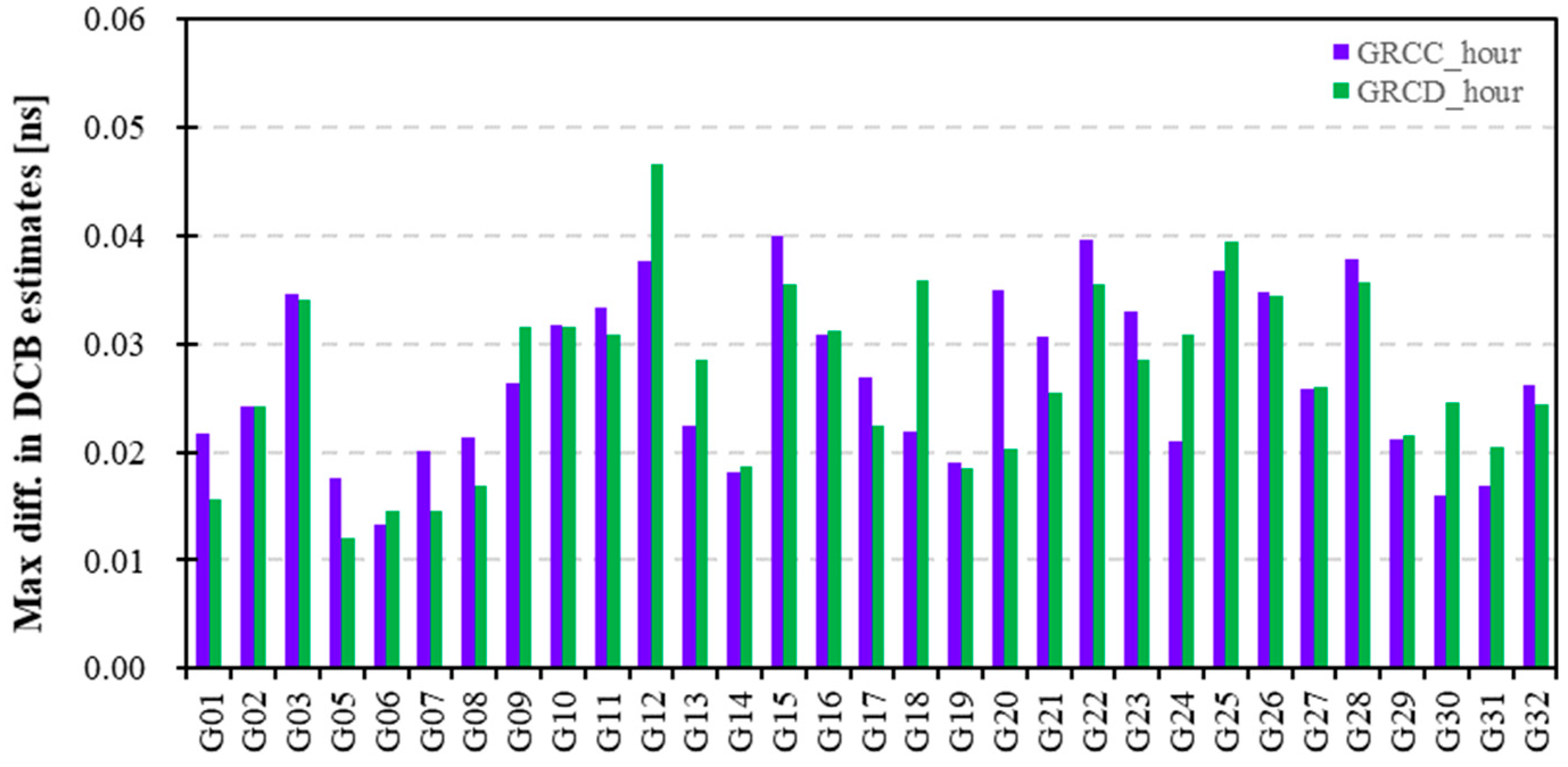
The mean DCB can exhibit the averaged ranges of DCBs in the form of specific and intuitive numbers; thereby, Table 1 presents the mean values of GPS satellite DCB estimates after adopting different modeling spacings of 2H, 4H, 6H, and 12H using the GRCC (a) and GRCD (b) observations. The GPS DCB values for G04 were not estimated owing to a lack of observations. The mean GPS DCB estimates range between −10 and 10 ns and are stable. There is no significant difference in mean GPS DCBs with different modeling spacings. Considering the limitation of mean statistics in Table 1 in terms of reflecting all DCB values, Figure 1 displays the maximum differences in the GPS satellite DCB estimates after adopting different modeling spacings using GRCC and GRCD observations during the experiment period. The differences in the GPS DCB estimates using different modeling spacings are in the range of 0.05 ns. Specifically, in Figure 1, the difference in G15 DCB estimates adopting different modeling spacings is the maximum value, 0.04 ns, when using GRCC data, whereas for GRCD data, the difference in G12 DCB is the largest, approximately 0.05 ns. Therefore, corresponding to Figure 1, the maximum, minimum, and differences in G15 and G12 DCB estimated based on different modeling spacings using GRCC and GRCD observations, respectively, are presented in Table 2. In Table 2a using GRCC data, the difference in the G15 DCB estimates based on different modeling spacings on DOY 5 is the largest, and the maximum, minimum, and difference are 2.6815, 2.6415, and 0.0400 ns, respectively. In Table 2b using GRCD data, the difference in G12 DCB estimated on DOY 4 is the largest, and the maximum, minimum, and difference are 4.3340, 4.2874, and 0.0466 ns, respectively. Therefore, there is a difference in the GPS DCB estimated using different modeling spacings, within 0.05 ns. The different modeling spacings affect the GPS DCB estimates.
3.1.2. Precision Evaluation of GPS Satellite DCB Estimates
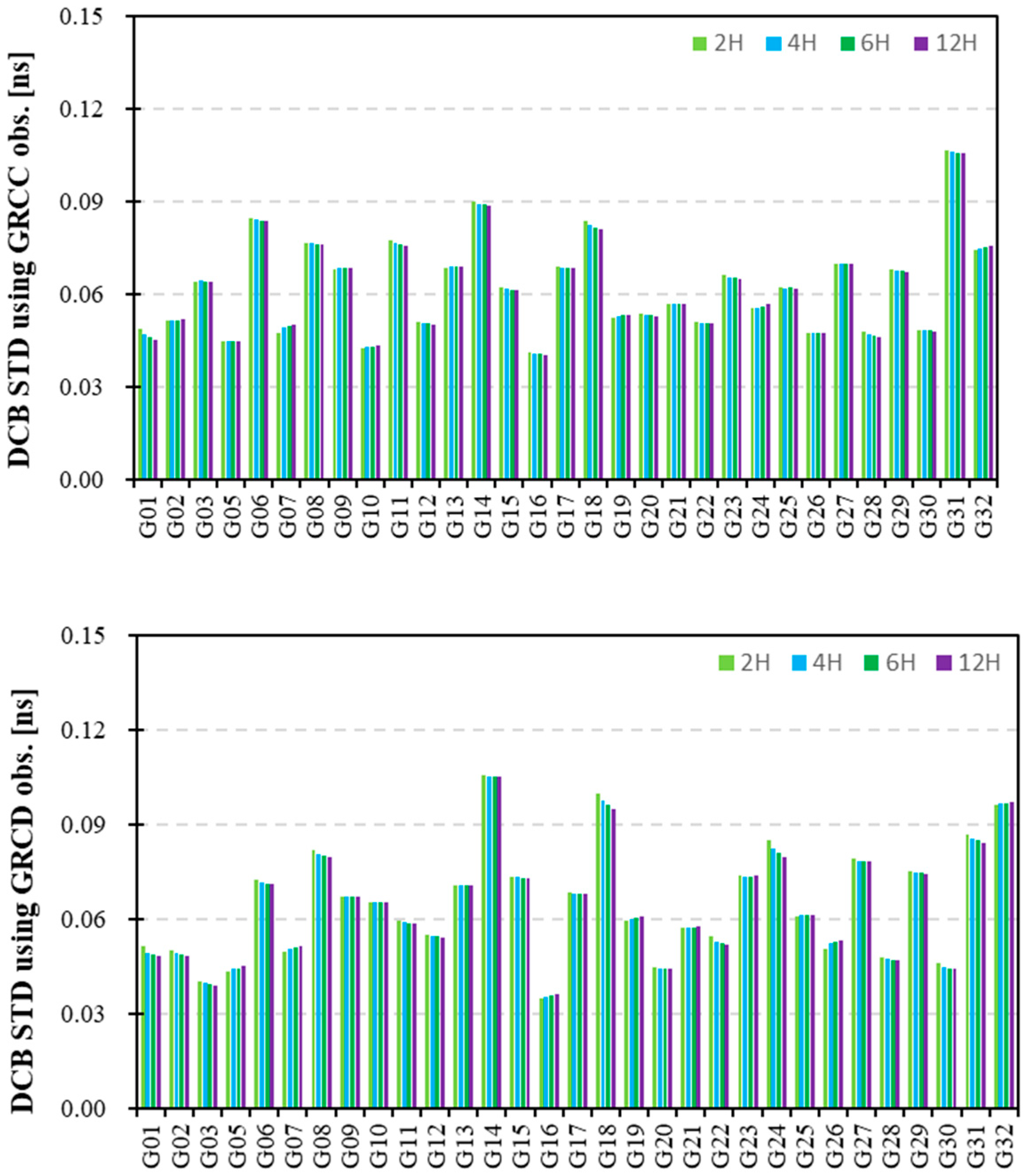
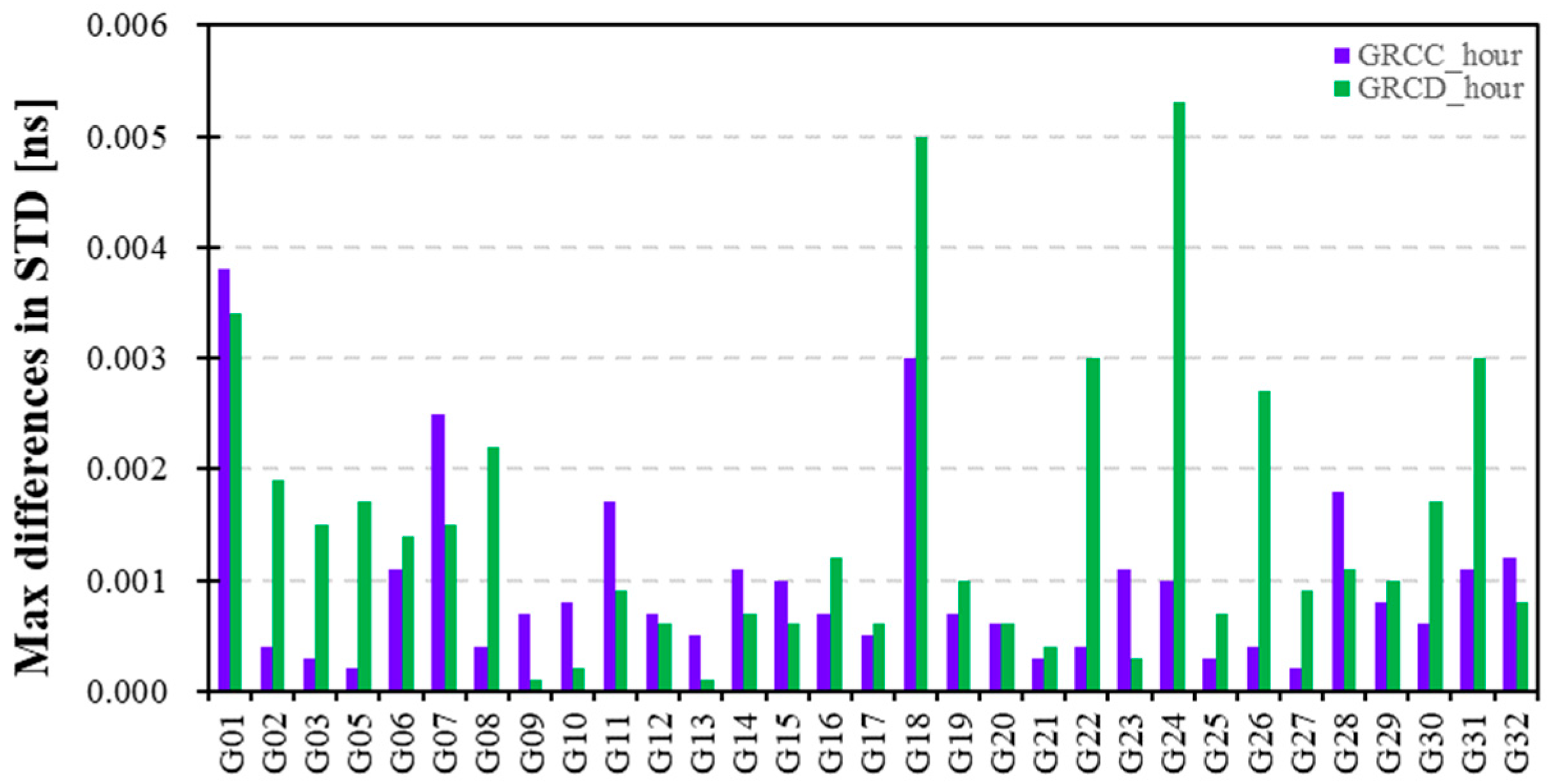
Figure 2 presents the monthly stabilities (STD) of the GPS satellite DCB estimates adopting different modeling spacings of 2H, 4H, 6H, and 12H using GRCC (top) and GRCD (bottom) observation data. The STDs of the GPS DCB estimates using GRCC and GRCD data are in the range of 0.11 ns with high stability. Meanwhile, the maximum differences in the STD of the GPS DCB estimates adopting different modeling spacings are shown in Figure 3. The maximum differences in the STD of the GPS DCB using different modeling spacings are within 0.006 ns. The STD values of the GPS DCB estimates adopting different modeling spacings exhibit no significant differences.
Table 3 presents the mean STDs of the GPS DCB estimates adopting the different modeling spacings. Statistically, the mean STD values of GPS DCBs with modeling spacings of 2H, 4H, 6H, and 12H using GRCC and GRCD data are 0.0624, 0.0621, 0.0620, and 0.0619 ns and 0.0648, 0.0643, 0.0641, and 0.0639 ns, respectively. The GPS DCB estimates with modeling spacings of 12H have the optimal mean STD results. The GPS DCB estimates using twin LEO satellite data attain similar and high stability.
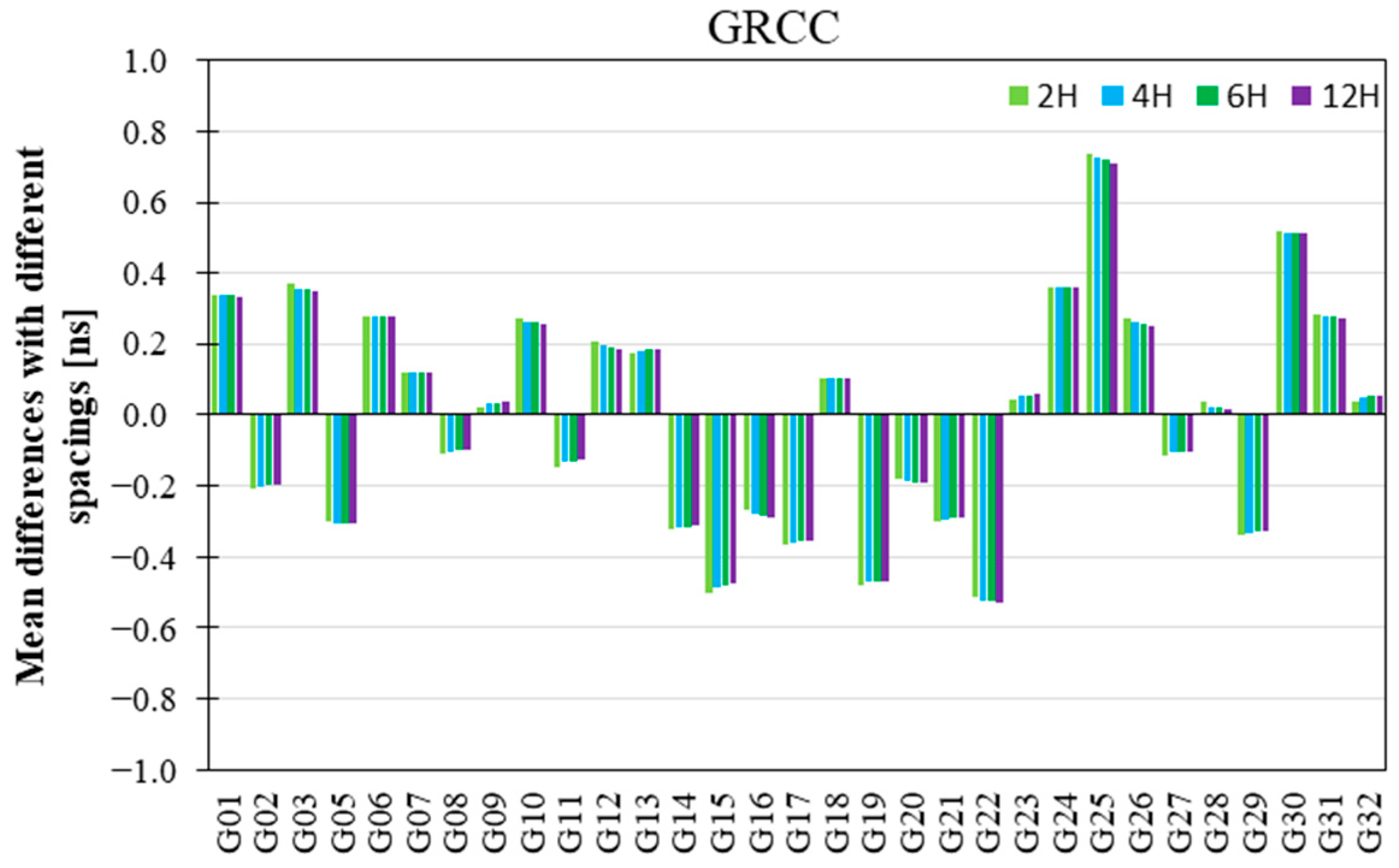
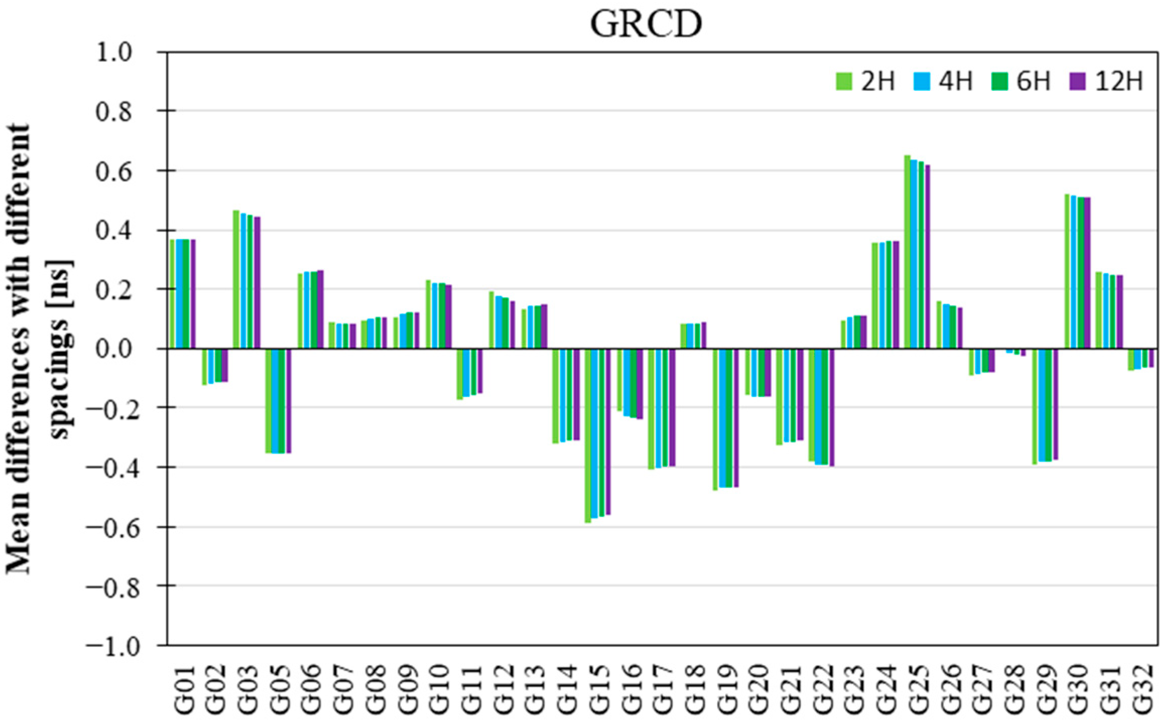
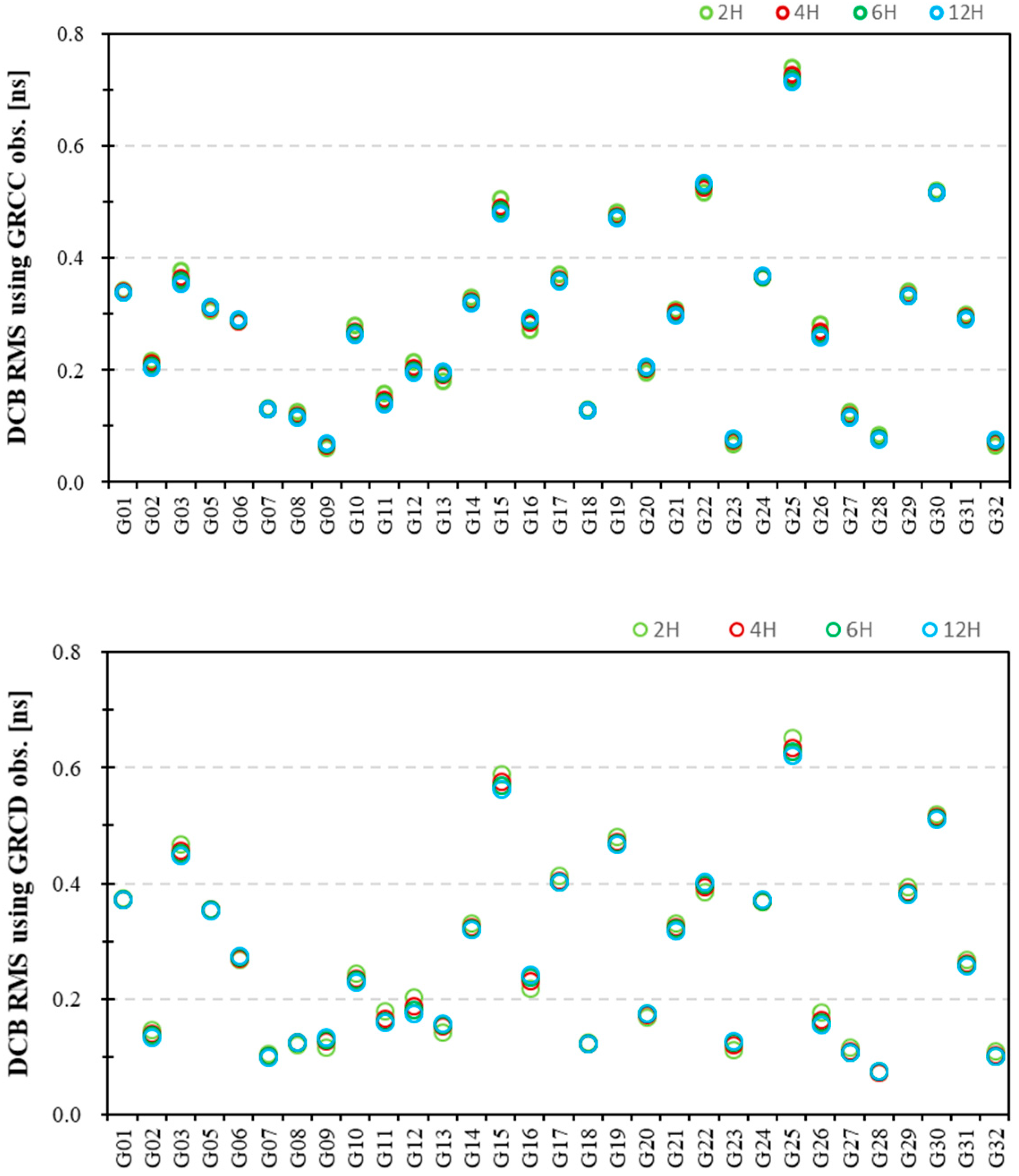
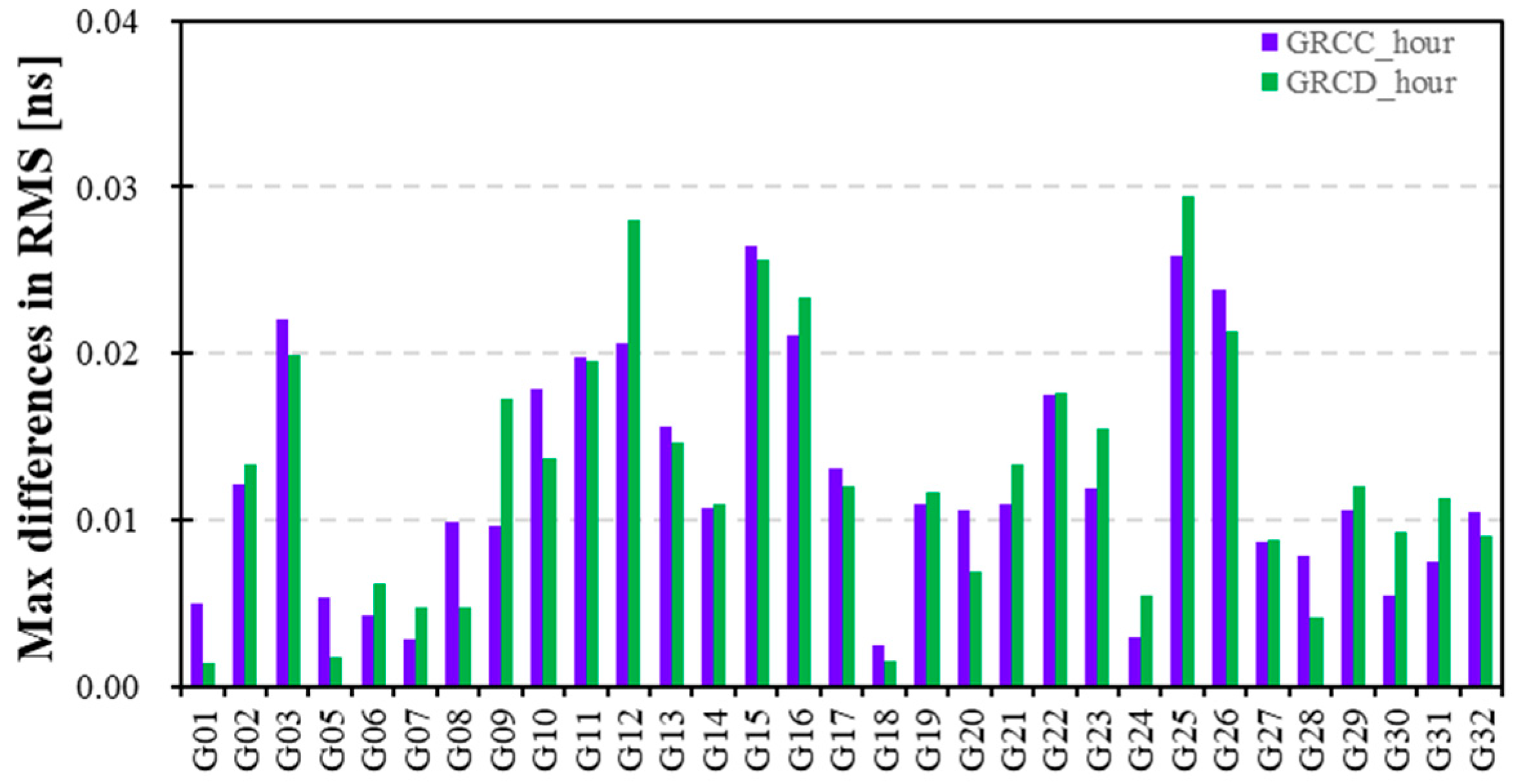
Figure 4 depicts the mean differences for GPS DCB estimates with different modeling spacings relative to CODE products. The mean differences in Figure 4 vary between −0.6 and 0.8 ns, which indicates that the GPS DCBs estimated by LEO satellite and ground station data have good consistency. Figure 5 showcases the RMS of the differences between the GPS DCB estimates adopting different modeling spacings (2H, 4H, 6H, and 12H) and the CODE DCB products. To visually demonstrate the differences in RMS of GPS DCBs with different modeling spacings, Figure 6 displays the maximum differences in RMS of GPS DCB estimates using different modeling spacings. The maximum differences in RMS of GPS DCBs using different modeling spacings are in the range of 0.03 ns. The different modeling spacings affect the RMS of the GPS DCB estimates. The corresponding mean RMS values are listed in Table 4. The RMS results of the GPS DCBs with different modeling spacings relative to the CODE products are in the range of 0.8 ns. The mean RMSs of the GPS DCBs are in the range of 0.3 ns, which indicates that the GPS DCBs estimated by LEO satellite and ground station data have good consistency. Statistically, the mean RMS results in Table 4 indicate that the GPS DCBs with a modeling spacing of 12H had slightly smaller RMS values than the others. Additionally, the GPS DCB estimates using twin satellite data have similar precisions, and the RMS results using GRCC observations are slightly poorer than those obtained using GRCD data.
3.1.3. LEO Receiver DCB Estimates and Stability Evaluation
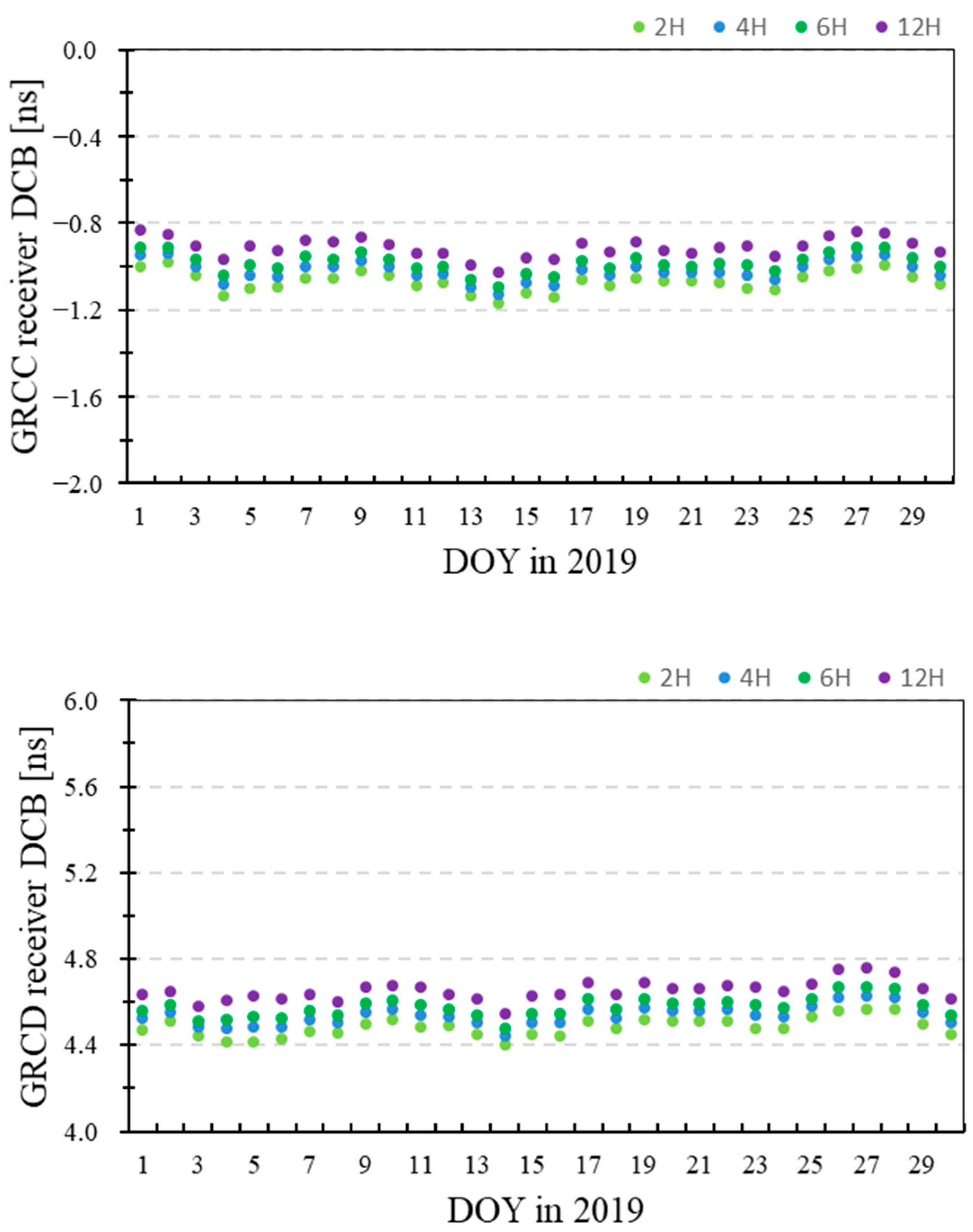
Figure 7 presents the time series of the receiver DCB estimates with modeling spacings of 2H, 4H, 6H, and 12H for the twin GRACE-FO satellites. The GRCC receiver DCB estimates are located at approximately −1.0 ns, whereas the GRCD DCB estimates fluctuate at approximately 4.6 ns, and their receiver DCB estimates are stable. In Figure 7, the GRCC and GRCD receiver DCB estimates are sorted in descending order as follows: receiver DCBs with modeling spacings of 12H, 6H, 4H, and 2H, where the receiver DCBs decrease as the modeling spacing decreases.
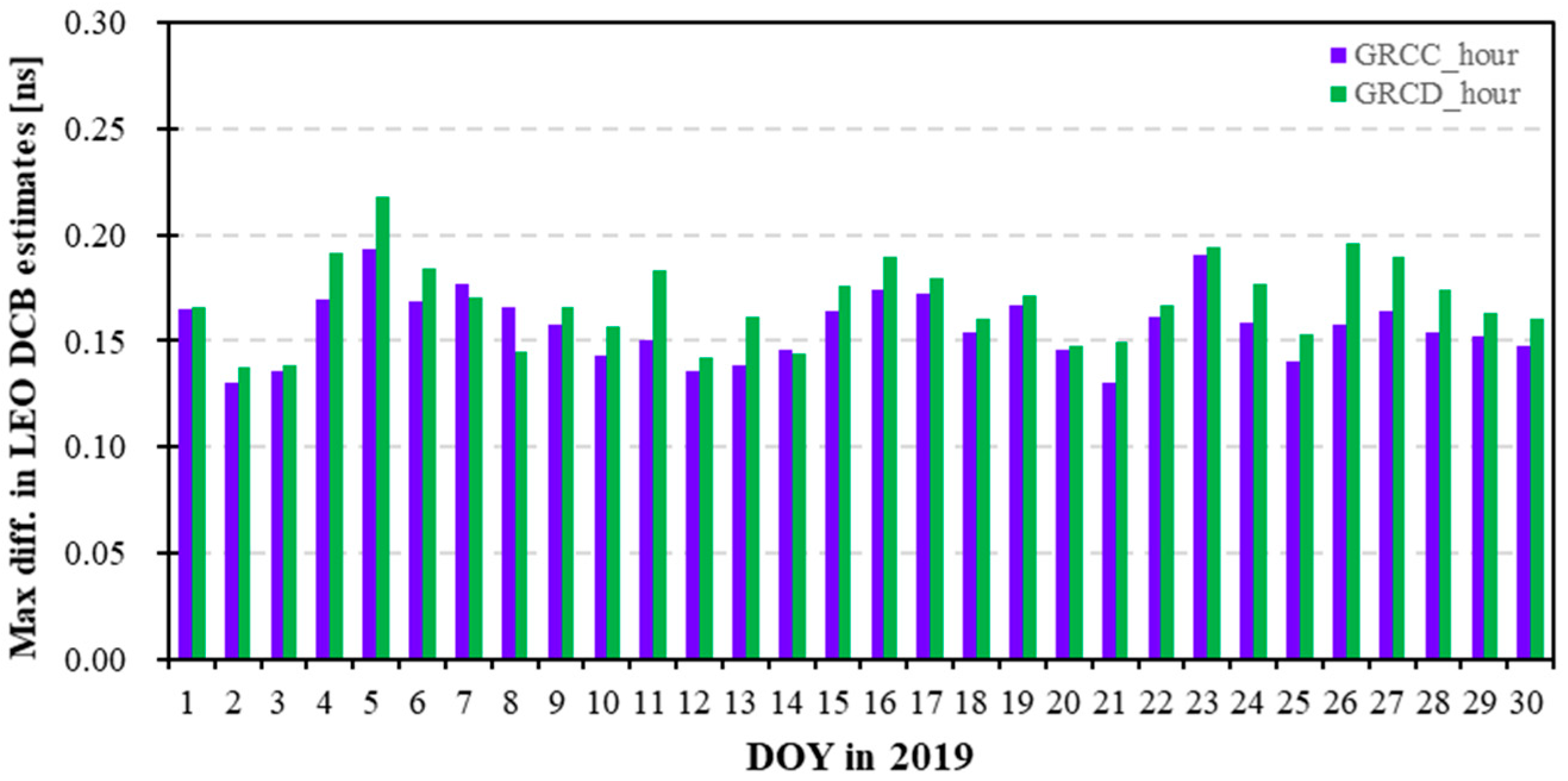
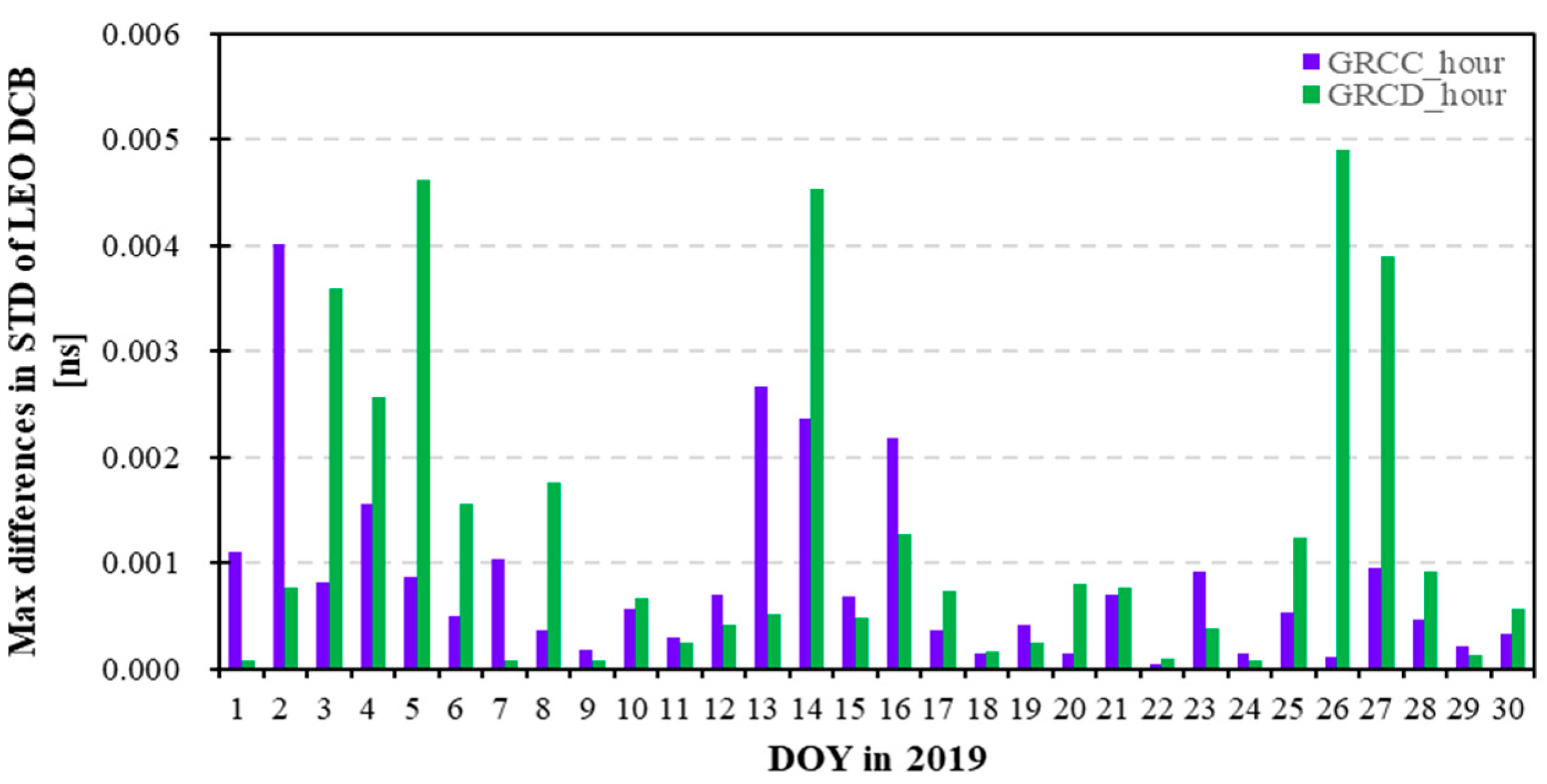
In order to visually demonstrate the differences in receiver DCBs with different modeling spacings, Figure 8 exhibits the maximum differences in the LEO receiver DCB estimates using different modeling spacings. Figure 9 shows the maximum differences in the STD of the receiver DCB using different modeling spacings. The maximum difference in receiver DCBs using different modeling spacings is 0.22 ns, whereas the maximum differences in STD of receiver DCBs are within 0.005 ns. This indicates that different modeling spacings have a significant impact on receiver DCB estimates.
The mean values and STD results for the LEO receiver DCB estimates with different modeling spacings are listed in Table 5. Statistically, the maximum receiver DCB values for both the GRCC and GRCD are the DCBs with modeling spacings of 12H, whereas the minimum receiver DCBs are those with modeling spacings of 2H. The differences in the mean receiver DCBs with different modeling spacings for the GRCC and GRCD are in the ranges of 0.1569 and 0.1684 ns, respectively. The GRCC and GRCD receiver DCBs achieve optimal STD results when modeling spacings of 6H and 4H are applied. The receiver DCBs of the twin GRACE-FO satellites are different; however, their DCB estimates have similar STD results.
In summary, the GPS DCB estimates using a modeling spacing of 12H have higher precision than the others, whereas LEO receiver DCBs applying the modeling spacings of 4H or 6H obtain optimal STD.
3.2. Different Modeling Degrees and Orders
This section investigates the impact of the D&O of spherical harmonic modeling on DCB estimates and precision, thereby obtaining suitable modeling D&O parameters. The 6, 8, and 10D&Os of spherical harmonic modeling were introduced into topside ionosphere modeling and DCB estimation. Subsequently, the GPS and LEO DCB estimates were analyzed and evaluated. The modeling spacing was fixed at 4H to improve the temporal resolution.
3.2.1. GPS Satellite DCB Estimates
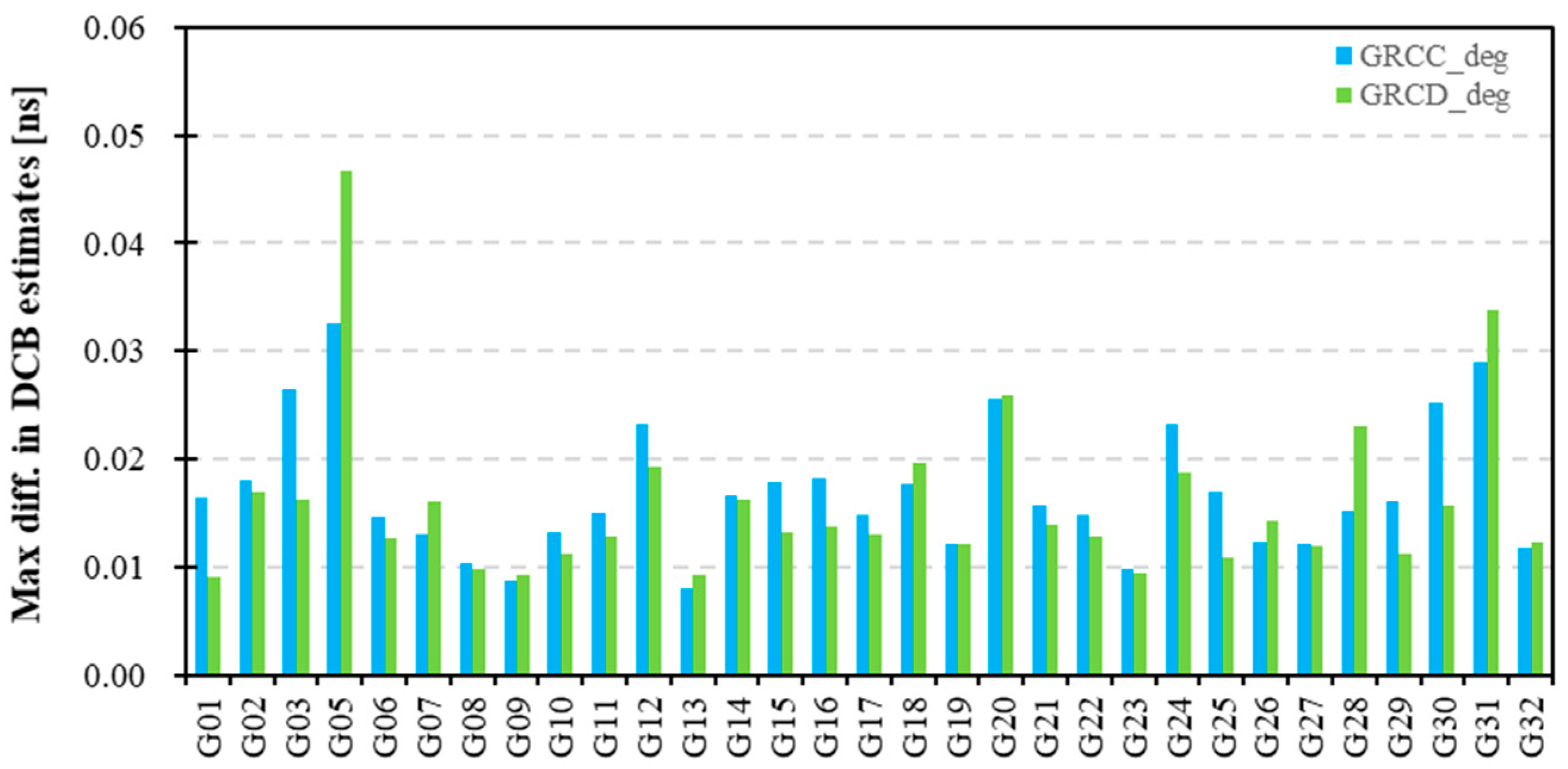
The mean values of GPS DCB estimates adopting different modeling parameters of 6, 8, and 10D&Os using the GRCC (a) and GRCD (b) observations are listed in Table 6. The GPS DCB values for G04 were not estimated owing to a lack of observations. The mean GPS DCB estimates range between −10 and 10 ns and are stable. There is no significant difference in the GPS DCB estimates obtained using different modeling D&Os. Considering the limitation of mean statistics in Table 6, Figure 10 exhibits the maximum differences in GPS DCB estimates adopting different modeling D&Os using GRCC and GRCD data. The differences in the GPS DCB estimates using different modeling D&Os are in the range of 0.05 ns. It indicates that the effects of the modeling spacing and D&O on GPS DCB estimates are at the same level. Specifically, the differences in G05 DCB estimates adopting different modeling D&Os using GRCC and GRCD data are both the largest, within 0.04 and 0.05 ns, respectively. The maximum, minimum, and differences in G05 DCB estimated with different modeling D&Os using GRCC and GRCD observations are presented in Table 7. In Table 7a, using GRCC data, the difference in G05 DCB estimates between different modeling D&Os on DOY 13 is the largest, and the maximum, minimum, and difference are 3.0099, 2.9776, and 0.0323 ns, respectively. In Table 7b, using GRCD data, the difference in G12 DCB estimated on DOY 4 is the largest, and the maximum, minimum, and difference are 3.0515, 3.0048, and 0.0467 ns, respectively. Therefore, there is a certain difference in the GPS DCB estimates using different modeling D&Os, all within 0.05 ns. The different modeling D&Os have certain effects on the GPS DCB estimates.
3.2.2. Precision Evaluation of GPS DCB Estimates
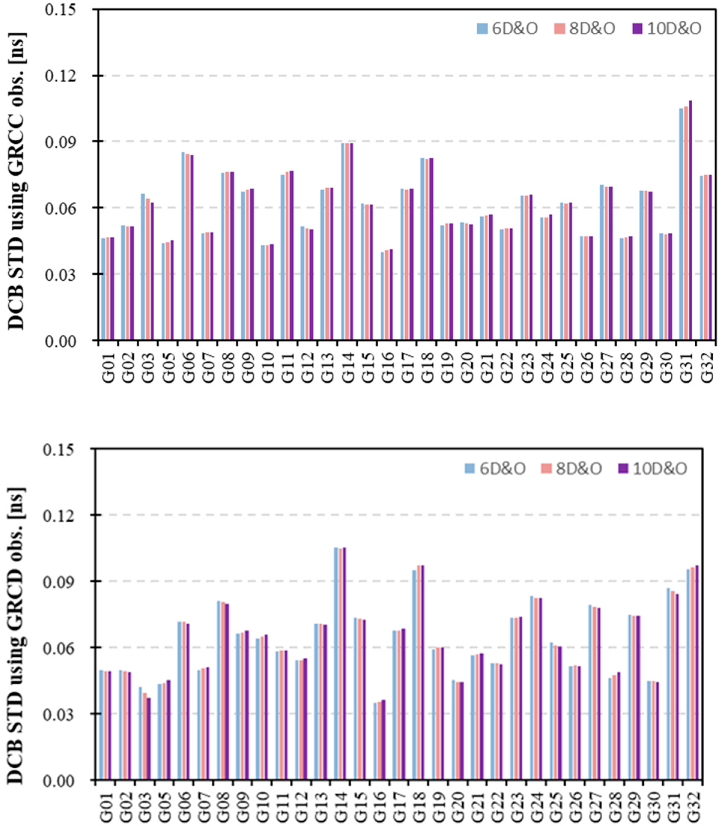
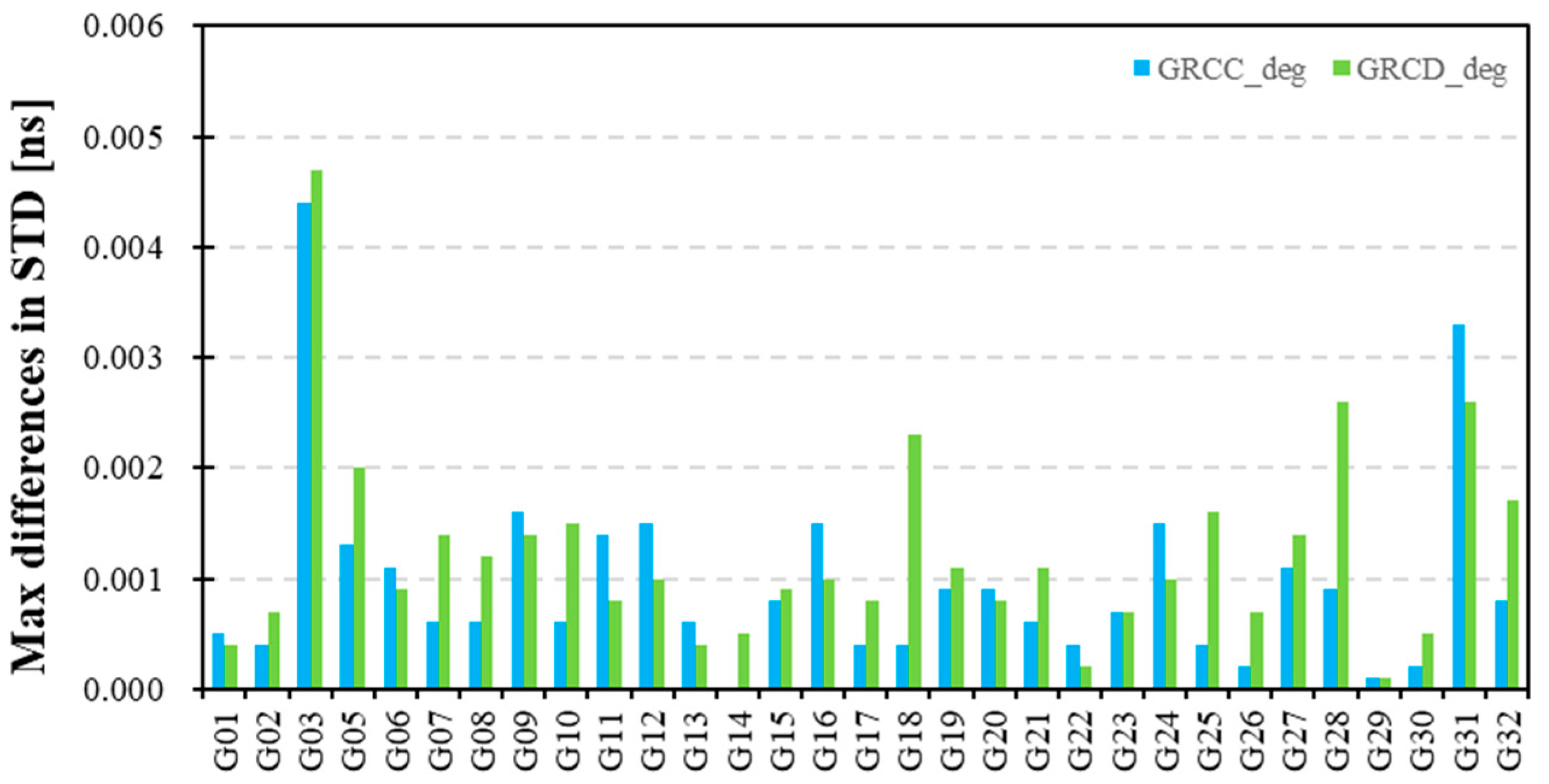
Figure 11 showcases the STD of GPS DCB estimates adopting different modeling D&Os of 6, 8, and 10 using GRCC and GRCD data. The STDs of GPS DCB estimates based on GRCC and GRCD data are within 0.11 ns. Additionally, Figure 12 displays the maximum differences in the STD of the GPS DCB estimates by applying different modeling D&Os. The maximum differences are within 0.005 ns. The STDs of the GPS DCB estimates adopting different modeling D&Os show no marked differences.
Table 8 presents the mean STDs of GPS satellite DCB estimates by applying different modeling D&Os. Statistically, the mean STD values of GPS DCBs with modeling D&Os of 6, 8, and 10 using GRCC and GRCD data are 0.0620, 0.0621, and 0.0623 ns and 0.0643, 0.0643, and 0.0644 ns, respectively. The GPS DCB estimates, with modeling D&Os of 6 and 8, attain the optimal STD results.
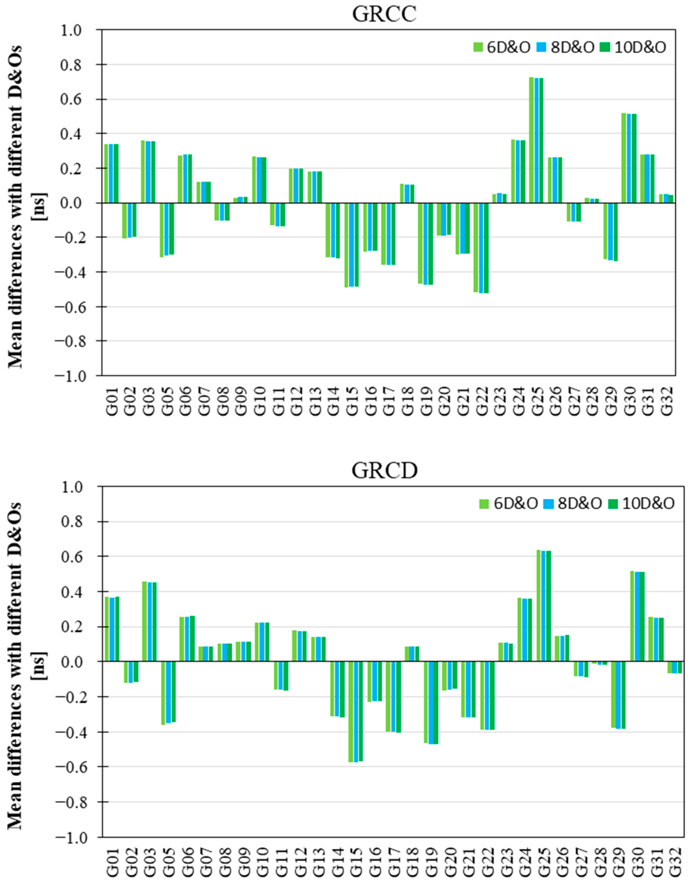
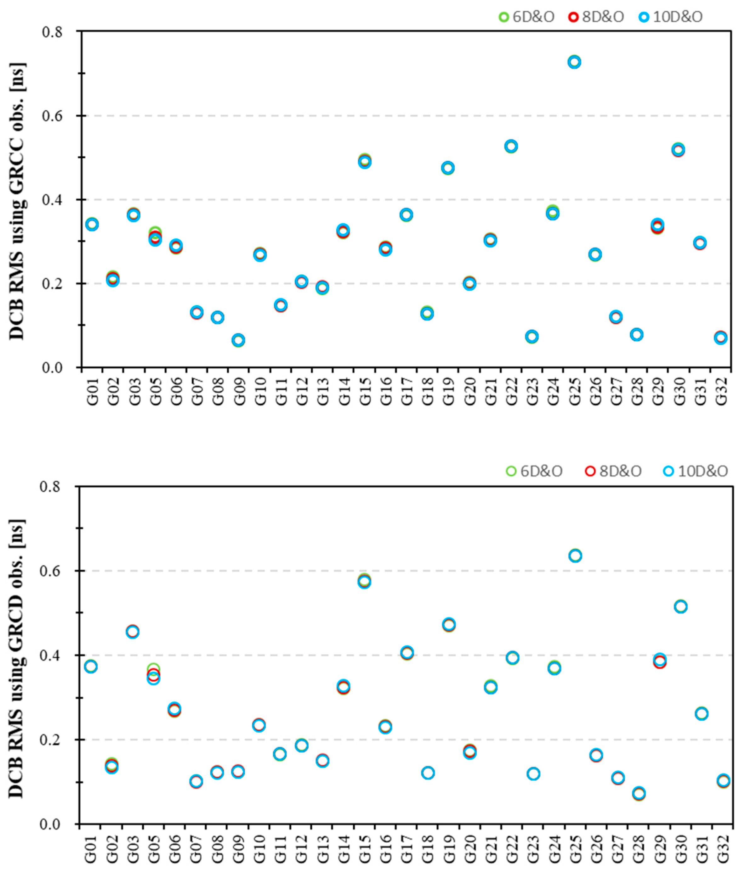
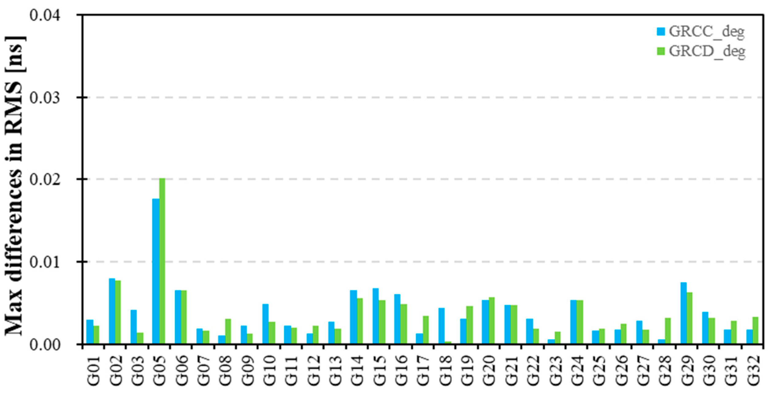
Figure 13 exhibits the mean differences for GPS DCB estimates with different D&Os relative to CODE products. The mean differences in Figure 13 vary between −0.6 and 0.7 ns, which indicates that the GPS DCBs estimated by LEO satellite and ground station data have good consistency. Figure 14 presents the RMS of the differences between the GPS DCB estimates adopting different modeling D&Os of 6, 8, and 10 and the CODE DCB products. To visually exhibit the differences in the RMS, Figure 15 displays the maximum differences in the RMS of the GPS DCB estimates using different modeling D&Os. The maximum differences reach 0.02 ns. The different modeling D&Os have certain effects on the RMS of the GPS DCB estimates. The corresponding mean RMS values are listed in Table 9. These RMS results are in the range of 0.8 ns. The mean RMS values are in the range of 0.3 ns, which indicates that the GPS DCBs estimated by LEO satellite and ground station data have good consistency. Statistically, Table 9 shows that the GPS DCBs with modeling D&Os of 8 and 10 have slightly higher RMS than the others. The RMS results using the GRCD observations are slightly higher than those obtained using the GRCC data. Considering the STD and RMS results of the GPS DCBs, the GPS DCB estimates with modeling D&Os of 8 attain superior precision.
3.2.3. LEO Receiver DCB Estimates and Stability Evaluation
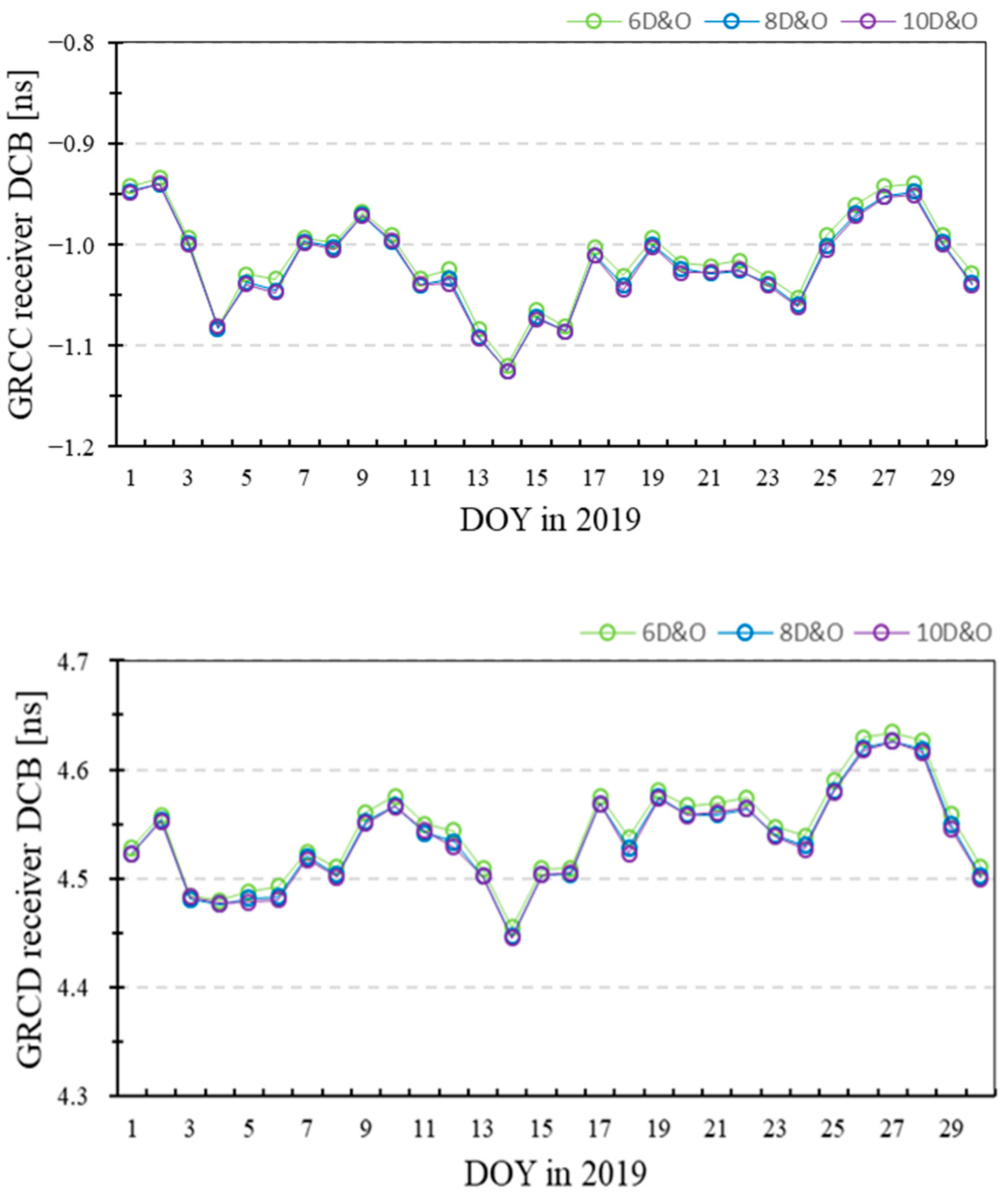
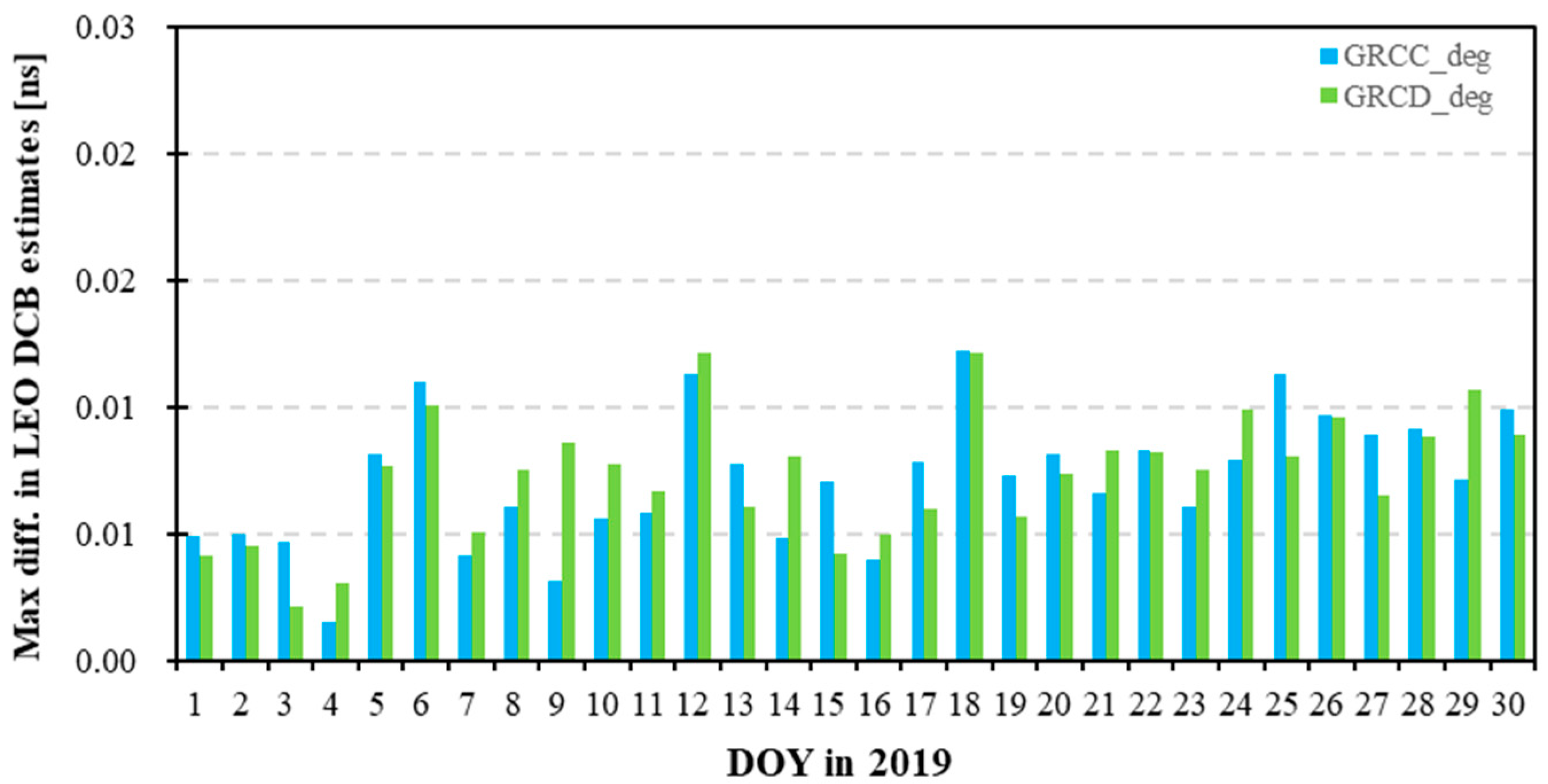
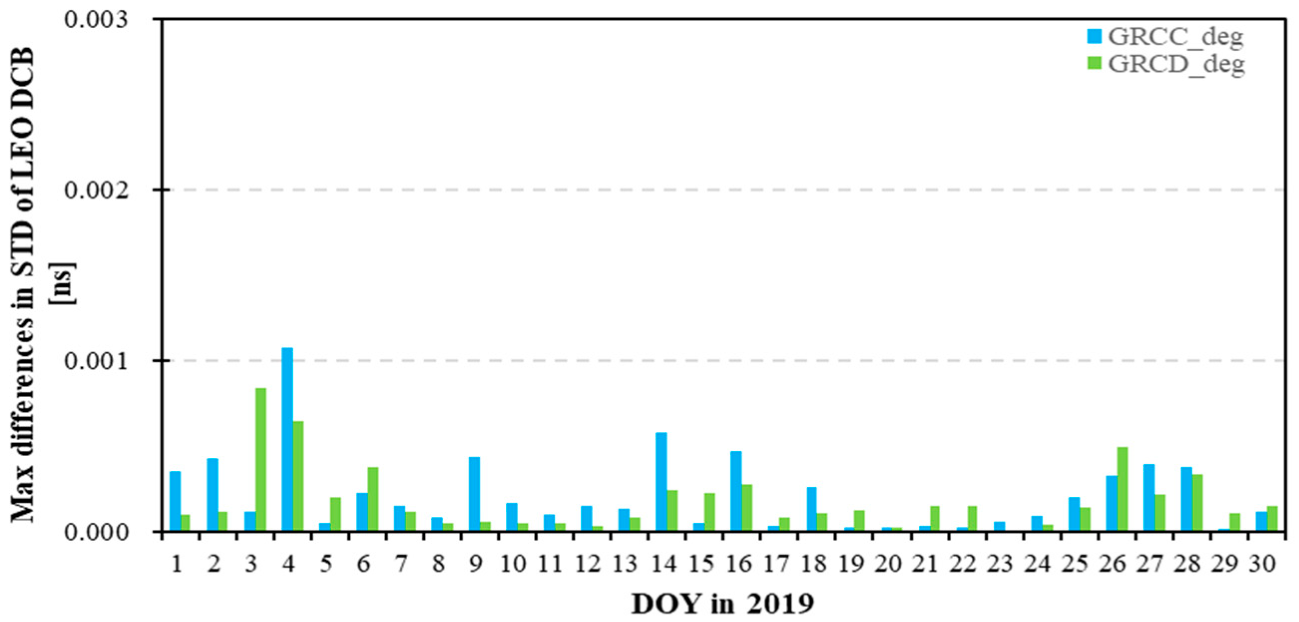
Figure 16 exhibits the time series of the receiver DCB estimates with different modeling D&Os of 6, 8, and 10 for twin GRACE-FO satellites. The GRCC receiver DCB estimates are located at approximately −1.0 ns, whereas the GRCD DCB estimates fluctuate at approximately 4.55 ns. The GRCC and GRCD receiver DCBs with the 6 D&O in spherical harmonic modeling are greater than the others. In order to visually present the differences in receiver DCBs with different modeling D&Os, Figure 17 shows the maximum differences in LEO DCB estimates using different modeling D&Os. Meanwhile, Figure 18 displays the maximum differences in the STD of the receiver DCB using different modeling D&Os. The maximum differences are within 0.02 ns, inferior to the differences in the GPS DCBs, while the maximum differences in STDs are within 0.002 ns.
The mean values and STD results for the receiver DCB estimates with different modeling D&Os are listed in Table 10. Statistically, the mean receiver DCBs for GRCC and GRCD are both sorted in descending order as follows: receiver DCBs with 6, 8, and 10D&Os modeling, where the receiver DCBs decrease as the modeling D&Os increase. The GRCC receiver DCBs with 10D&O modeling gain the minimum STD result, whereas the GRCD DCBs applying 8 and 10D&Os have a better STD than the others. The receiver DCBs of the GRCC and GRCD differ; however, their DCB estimates have similar STD results.
In summary, adopting 8D&O in the LEO-based VTEC modeling exhibits superior estimates and precisions for both GPS and LEO DCBs. Additionally, compared to the results in Section 3.1, this demonstrates that the impact of modeling spacing on DCB estimates is greater than that of modeling D&O.
4. Conclusions
The effects of topside ionosphere VTEC modeling parameters on LEO-based DCB estimates and precision were investigated using GRACE-FO observation data to obtain superior modeling parameters. Different modeling parameters were set into the DCB estimations, encompassing the modeling spacing in the dynamic temporal mode and D&O in LEO-based VTEC modeling. The differences in GPS and LEO DCB estimates with the different modeling parameters were showcased, the precision of the DCB estimates was evaluated, and the effects of these parameters on DCB estimation were analyzed. The beneficial conclusions are drawn as follows:
(1) The mean GPS DCB estimates range between −10 and 10 ns. Although there is no significant difference in the mean GPS DCB estimates obtained using different modeling spacings, the mean DCB may have a limitation in reflecting all real DCBs. The maximum differences in the GPS DCB estimates after adopting different modeling spacings reach 0.05 ns. The different modeling spacings affect the GPS DCB estimates. The maximum differences in the RMS with different modeling spacings are in the range of 0.03 ns. The different modeling spacings have certain effects on the RMS of the GPS DCBs. The GPS DCB estimates with a modeling spacing of 12H have slightly higher precisions than the others.
The maximum difference in receiver DCBs adopting different modeling spacings is 0.22 ns, which indicates that modeling spacing has a significant impact on the receiver DCBs compared with GPS DCBs. The GRCC and GRCD receiver DCBs gain more optimal STD than the others when applying modeling spacings of 6H and 4H, respectively.
In summary, the GPS DCB estimates using a modeling spacing of 12H have higher precisions than the others, whereas LEO DCBs applying the modeling spacings of 4H or 6H obtain optimal STD results.
(2) The differences in the GPS DCB estimates using different modeling D&Os of 6, 8, and 10 are also in the range of 0.05 ns. The different modeling D&Os affect the GPS DCB estimates. The maximum difference in the RMS with different modeling spacings is 0.02 ns. The GPS DCB estimates, with a modeling D&O of 8, attain superior STD and RMS values.
In terms of receiver DCBs, the maximum differences in receiver DCBs using different modeling D&Os are within 0.02 ns, inferior to the differences in the GPS DCBs. The GRCC and GRCD DCBs achieve the optimal STD when adopting modeling D&Os of 10 and 8, respectively.
In summary, adopting 8D&O in the LEO-based VTEC modeling can obtain superior estimates and precisions for both GPS and LEO DCBs.
(3) The modeling spacing has a greater effect on the LEO receiver DCBs than on the GPS DCBs. The effects of the different modeling spacings and D&Os on the GPS DCB estimates and their RMS are at the same level. The modeling spacing has a greater impact on the LEO receiver DCBs than those of the modeling D&O. The research conclusions in this study can provide references for estimating the GNSS and LEO satellite DCBs using LEO onboard observation data.
Author Contributions
In this work, M.L. proposed the idea, designed the experiment results, and provided the software; Y.W. collected the experimental data; Y.W. and M.L. analyzed the experiment results and completed the paper. Y.Y., G.W. and H.G. supervised its analysis and edited the manuscript. All authors have read and agreed to the published version of the manuscript.
Funding
This work was supported by the China Postdoctoral Science Foundation (2021MD703896), supported by the Science and technology project of China Southern Power Grid Yunnan Power Grid Co., Ltd. (YNKJXM20220033), the China Natural Science Funds (No. 42074045, 42374043), and the Independent Project of the State Key Laboratory of China.
Data Availability Statement
CODE precise products are available at ftp://ftp.aiub.unibe.ch/ (accessed on 27 February 2023); onboard GPS observation data of the GRACE-FO satellites are available at ftp://rz-vm152.gfz-potsdam.de/ (accessed on 27 February 2023).
Acknowledgments
The authors are grateful to CODE for providing the precise products and onboard GPS observation data of GRACE-FO satellites, respectively. Meanwhile, we would like to thank the anonymous reviewers for their valuable comments.
Conflicts of Interest
The authors declare that this study received funding from China Southern Power Grid Yunnan Power Grid Co., Ltd. (YNKJXM20220033). The funder had the following involvement with the study: Yifan Wang and Mingming Liu analyzed the experiment results and completed the paper, Yunbin Yuan, Guofang Wang, and Hao Geng supervised its analysis and edited the manuscript.
References
- Schaer, S. Mapping and Predicting the Earth’s Ionosphere Using the Global Positioning System. Ph.D. Dissertation, University of Berne, Bern, Switzerland, 1999. [Google Scholar]
- Yuan, Y. Study on Theories and Methods of Correcting Ionospheric Delay and Monitoring Ionosphere Based on GPS. Ph.D. Dissertation, Institute of Geodesy and Geophysics, Chinese Academy of Sciences, Wuhan, China, 2002. [Google Scholar]
- Dach, R.; Schaer, S.; Hugentobler, U.; Schildknecht, T.; Gäde, A. Combined multi-system GNSS analysis for time and frequency transfer. In Proceedings of the 20th European Frequency and Time Forum, Braunschweig, Germany, 27–30 March 2006; pp. 530–537. [Google Scholar]
- Hernández-Pajares, M.; Juan, J.M.; Sanz, J.; Aragón-Àngel, À.; García-Rigo, A.; Salazar, D.; Escudero, M. The ionosphere: Effects, GPS modeling and the benefits for space geodetic techniques. J. Geod. 2011, 85, 887–907. [Google Scholar] [CrossRef]
- Montenbruck, O.; Hauschild, A. Code biases in multi-GNSS point positioning. In Proceedings of the 2013 International Technical Meeting of the Institute of Navigation, San Diego, CA, USA, 27–29 January 2013. [Google Scholar]
- Montenbruck, O.; Hauschild, A.; Steigenberger, P. Diferential code bias estimation using Multi-GNSS observations and global ionosphere maps. Navigation 2014, 61, 191–201. [Google Scholar] [CrossRef]
- Wang, N.; Yuan, Y.; Li, Z.; Montenbruck, O.; Tan, B. Determination of differential code biases with multi-GNSS observations. J. Geod. 2016, 90, 209–228. [Google Scholar] [CrossRef]
- Liu, T.; Zhang, B. Estimation of code observation-specific biases (OSBs) for the modernized multi-frequency and multi-GNSS signals: An undifferenced and uncombined approach. J. Geod. 2021, 95, 97. [Google Scholar] [CrossRef]
- Mannucci, A.; Wilson, B.; Yuan, D.; Ho, C.; Lindqwister, U.; Runge, T. A global mapping technique for GPS-derived ionospheric total electron content measurements. Radio Sci. 1998, 33, 565–582. [Google Scholar] [CrossRef]
- Schaer, S.; Gurtner, W.; Feltens, J. IONEX: The ionosphere map exchange format version 1. In Proceedings of the IGS AC Workshop, Darmstadt, Germany, 9–11 February 1998. [Google Scholar]
- Schaer, S. Differential code biases (DCB) in GNSS analysis. In Proceedings of the IGS Workshop, Miami Beach, FL, USA, 2–6 June 2008. [Google Scholar]
- Schaer, S. Activities of IGS Bias and Calibration Working Group. In IGS Technical Report 2011; Meindl, M., Dach, R., Jean, Y., Eds.; Astronomical Institute, University of Berne: Berne, Switzerland, 2012; pp. 139–154. [Google Scholar]
- Krankowski, A.; Shagimuratov, I.I.; Ephishov, I.I.; Krypiak-Gregorczyk, A.; Yakimova, G. The occurrence of themid-latitude ionospheric trough in GPS-TEC measurements. Adv. Space Res. 2009, 43, 1721–1731. [Google Scholar] [CrossRef]
- Yuan, Y.; Ou, J. A generalized trigonometric series function model for determining ionospheric delay. Prog. Nat. Sci. 2004, 14, 1010–1014. [Google Scholar] [CrossRef]
- Li, Z.; Yuan, Y.; Li, H.; Ou, J.; Huo, X. Two-step method for the determination of the differential code biases of COMPASS satellites. J. Geod. 2012, 86, 1059–1076. [Google Scholar] [CrossRef]
- Lin, J.; Yue, X.; Zhao, S. Estimation and analysis of GPS satellite DCB based on LEO observations. GPS Solut. 2014, 20, 251–258. [Google Scholar] [CrossRef]
- Zhong, J.; Lei, J.; Dou, X.; Yue, X. Is the long-term variation of the estimated GPS differential code biases associated with ionospheric variability? GPS Solut. 2015, 20, 313–319. [Google Scholar] [CrossRef]
- Jin, R.; Jin, S.; Feng, G. M_DCB: Matlab code for estimating GNSS satellite and receiver differential code biases. GPS Solut. 2012, 16, 541–548. [Google Scholar] [CrossRef]
- Wautelet, G.; Loyer, S.; Mercier, F.; Perosanz, F. Computation of GPS P1–P2 Differential Code Biases with JASON-2. GPS Solut. 2017, 21, 1619–1631. [Google Scholar] [CrossRef]
- Chen, P.; Yao, Y.; Li, Q.; Yao, W. Modeling the plasmasphere based on LEO satellites onboard GPS measurements. J. Geophys. Res. Space Phys. 2017, 122, 1221–1233. [Google Scholar] [CrossRef]
- Li, W.; Li, M.; Shi, C.; Fang, R.; Zhao, Q.; Meng, X.; Bai, W. GPS and BeiDou Differential Code Bias Estimation Using Fengyun-3C Satellite Onboard GNSS Observations. Remote Sens. 2017, 9, 1239. [Google Scholar] [CrossRef]
- Li, X.; Ma, T.; Xie, W.; Zhang, K.; Huang, J.; Ren, X. FY-3D and FY-3C onboard observations for differential code biases estimation. GPS Solut. 2019, 23, 57. [Google Scholar] [CrossRef]
- Zhou, P.; Nie, Z.; Xiang, Y.; Wang, J.; Du, L.; Gao, Y. Differential code bias estimation based on uncombined PPP with LEO onboard GPS observations. Adv. Space Res. 2019, 65, 541–551. [Google Scholar] [CrossRef]
- Ren, X.; Chen, J.; Zhang, X.; Schmidt, M.; Li, X.; Zhang, J. Mapping topside ionospheric vertical electron content from multiple LEO satellites at different orbital altitudes. J. Geod. 2020, 94, 86. [Google Scholar] [CrossRef]
- Liu, M.; Yuan, Y.; Huo, X.; Li, M.; Chai, Y. Simultaneous estimation of GPS P1–P2 differential code biases using low earth orbit satellites data from two different orbit heights. J. Geod. 2020, 94, 121. [Google Scholar] [CrossRef]
- Zakharenkova, I.; Cherniak, I. How can GOCE and TerraSAR-X contribute to the topside ionosphere and plasmasphere research? Space Weather 2015, 13, 271–285. [Google Scholar] [CrossRef]
- Zhong, J.; Lei, J.; Yue, X.; Dou, X. Determination of differential code bias of GNSS receiver onboard low earth orbit satellite. IEEE Trans. Geosci. Remote Sens. 2016, 54, 4896–4905. [Google Scholar] [CrossRef]
- Zhang, X.; Tang, L. Estimation of COSMIC LEO satellite GPS receiver differential code bias. Chin. J. Geophys. 2014, 57, 377–383. [Google Scholar]
- Wen, H.; Kruizingga, G.; Paik, M.; Landerer, F.; Bertiger, W.; Sakumura, C.; Bandikova, T.; Mccullough, C. Gravity Recovery and Climate Experiment Follow-On (GRACE-FO) Level-1 Data Product User Handbook; NASA: Silicon Valley, CA, USA, 2019. [Google Scholar]
- Foelsche, U.; Kirchengast, G. A simple “geometric” mapping function for the hydrostatic delay at radio frequencies and assessment of its performance. Geophys. Res. Lett. 2002, 29, 111-1–111-4. [Google Scholar] [CrossRef]
- Yue, X.; Schreiner, W.S.; Hunt, D.C.; Rocken, C.; Kuo, Y.H. Quantitative evaluation of the low Earth orbit satellite based slant total electron content determination. Space Weather 2011, 9, S09001. [Google Scholar] [CrossRef]
- Zhong, J.; Lei, J.; Dou, X.; Yue, X. Assessment of vertical TEC mapping functions for space-based GNSS observations. GPS Solut. 2015, 20, 353–362. [Google Scholar] [CrossRef]
- Klobuchar, J.A. A First-Order World-Wide Ionospheric Time-Delay Algorithm; Air Force Cambridge Research Labs.: Bedford, MA, USA, 1975; No. 324. [Google Scholar]
- IGS. IGS Technical Report 2011; Astronomical Institute, University of Berne: Berne, Switzerland, 2012. [Google Scholar]
- Sanz, J.; Miguel-Juan, J.; Rovira-Garcia, A.; Gonza’lez-Casado, G. GPS differential code biases determination: Methodology and analysis. GPS Solut. 2017, 21, 1549–1561. [Google Scholar] [CrossRef]
- Jäggi, A.; Hugentobler, U.; Beutler, G. Pseudo-Stochastic orbit modeling techniques for Low-Earth Orbiters. J. Geod. 2006, 80, 47–60. [Google Scholar] [CrossRef]
- Kang, Z.; Tapley, B.; Bettadpur, S.; Ries, J.; Nagel, P.; Pastor, R. Precise orbit determination for the GRACE mission using only GPS data. J. Geod. 2006, 80, 322–331. [Google Scholar] [CrossRef]
- Montenbruck, O.; Andres, Y.; Bock, H.; van Helleputte, T.; van den Ijssel, J.; Loiselet, M.; Marquardt, C.; Silvestrin, P.; Visser, P.; Yoon, Y. Tracking and orbit determination performance of the GRAS instrument on MetOp-A. GPS Solut. 2008, 12, 289–299. [Google Scholar] [CrossRef]
- Hwang, C.; Tseng, T.-P.; Lin, T.; Švehla, D.; Schreiner, B. Precise orbit determination for the FORMOSAT-3/COSMIC satellite mission using GPS. J. Geod. 2008, 83, 477–489. [Google Scholar] [CrossRef]
- Cerri, L.; Berthias, J.P.; Bertiger, W.I.; Haines, B.J.; Lemoine, F.G.; Mercier, F.; Ries, J.C.; Willis, P.; Zelensky, N.P.; Ziebart, M. Precision Orbit Determination Standards for the Jason Series of Altimeter Missions. Mar. Geod. 2010, 33, 379–418. [Google Scholar] [CrossRef]
- Liu, M.; Yuan, Y.; Ou, J.; Chai, Y. Research on Attitude Models and Antenna Phase Center Correction for Jason-3 Satellite Orbit Determination. Sensors 2019, 19, 2408. [Google Scholar] [CrossRef] [PubMed]
Figure 1.
Maximum differences in GPS DCB estimates adopting different modeling spacings using twin LEO observations.
Figure 1.
Maximum differences in GPS DCB estimates adopting different modeling spacings using twin LEO observations.

Figure 2.
Monthly stability (STD) of GPS DCB estimates adopting different modeling spacings ((top): GRCC and (below): GRCD data).
Figure 2.
Monthly stability (STD) of GPS DCB estimates adopting different modeling spacings ((top): GRCC and (below): GRCD data).

Figure 3.
Maximum differences in STD of GPS DCB estimates adopting different modeling spacings.

Figure 4.
Mean differences for GPS DCBs using different spacings relative to CODE products.


Figure 5.
Root-mean square (RMS) for differences between the GPS DCB estimates using different modeling spacings and CODE DCB products ((top): GRCC and (below): GRCD data).
Figure 5.
Root-mean square (RMS) for differences between the GPS DCB estimates using different modeling spacings and CODE DCB products ((top): GRCC and (below): GRCD data).

Figure 6.
Maximum differences in RMS of the GPS DCB estimates using different modeling spacings.

Figure 7.
GRACE-FO receiver DCB estimates with different modeling spacings ((top): GRCC and (below): GRCD).
Figure 7.
GRACE-FO receiver DCB estimates with different modeling spacings ((top): GRCC and (below): GRCD).

Figure 8.
Maximum differences in LEO DCB estimates using different modeling spacings.

Figure 9.
Maximum differences in STD of LEO DCB estimates using different spacings.

Figure 10.
Maximum differences in GPS DCB estimates adopting different D&Os using twin LEO observations.
Figure 10.
Maximum differences in GPS DCB estimates adopting different D&Os using twin LEO observations.

Figure 11.
Monthly stability of GPS satellite DCB estimates using different modeling D&Os ((top): GRCC obs. and (below): GRCD obs.).
Figure 11.
Monthly stability of GPS satellite DCB estimates using different modeling D&Os ((top): GRCC obs. and (below): GRCD obs.).

Figure 12.
Maximum differences in STD of GPS DCB estimates using different D&Os.

Figure 13.
Mean differences for GPS DCBs using different D&Os relative to CODE products.

Figure 14.
RMS of differences between the GPS DCB estimates using different modeling D&Os and CODE DCB products ((top): GRCC data and (below): GRCD data).
Figure 14.
RMS of differences between the GPS DCB estimates using different modeling D&Os and CODE DCB products ((top): GRCC data and (below): GRCD data).

Figure 15.
Maximum differences in RMS of the GPS DCB estimates using different D&Os.

Figure 16.
GRACE-FO receiver DCB estimates adopting different modeling D&Os ((top): GRCC and (below): GRCD).
Figure 16.
GRACE-FO receiver DCB estimates adopting different modeling D&Os ((top): GRCC and (below): GRCD).

Figure 17.
Maximum differences in LEO DCB estimates using different modeling D&Os.

Figure 18.
Maximum differences in STD of LEO DCB estimates using different D&Os.


Table 1.
Mean GPS differential code bias (DCB) estimates based on different modeling spacings using GRCC (a) and GRCD (b) observations [ns].
Table 1.
Mean GPS differential code bias (DCB) estimates based on different modeling spacings using GRCC (a) and GRCD (b) observations [ns].
| (a) GRCC | ||||
| GPS | 2H | 4H | 6H | 12H |
| G01 | −7.4145 | −7.4174 | −7.4183 | −7.4191 |
| G02 | 9.1243 | 9.1298 | 9.1330 | 9.1375 |
| G03 | −5.0039 | −5.0161 | −5.0208 | −5.0262 |
| G05 | 2.9826 | 2.9782 | 2.9775 | 2.9772 |
| G06 | −6.6772 | −6.6762 | −6.6750 | −6.6726 |
| G07 | 3.3569 | 3.3536 | 3.3532 | 3.3534 |
| G08 | −7.5298 | −7.5226 | −7.5205 | −7.5182 |
| G09 | −4.9578 | −4.9469 | −4.9431 | −4.9388 |
| G10 | −5.0343 | −5.0449 | −5.0487 | −5.0529 |
| G11 | 3.7213 | 3.7332 | 3.7374 | 3.7420 |
| G12 | 4.1600 | 4.1480 | 4.1436 | 4.1385 |
| G13 | 3.4175 | 3.4277 | 3.4307 | 3.4336 |
| G14 | 1.9124 | 1.9205 | 1.9223 | 1.9231 |
| G15 | 2.6321 | 2.6467 | 2.6523 | 2.6588 |
| G16 | 2.7966 | 2.7844 | 2.7801 | 2.7753 |
| G17 | 2.9321 | 2.9406 | 2.9429 | 2.9452 |
| G18 | −0.2903 | −0.2915 | −0.2913 | −0.2908 |
| G19 | 5.6329 | 5.6405 | 5.6425 | 5.6440 |
| G20 | 1.4707 | 1.4640 | 1.4621 | 1.4597 |
| G21 | 2.2743 | 2.2791 | 2.2821 | 2.2857 |
| G22 | 7.2749 | 7.2648 | 7.2612 | 7.2572 |
| G23 | 9.1329 | 9.1434 | 9.1469 | 9.1511 |
| G24 | −5.5552 | −5.5542 | −5.5536 | −5.5526 |
| G25 | −7.1077 | −7.1219 | −7.1273 | −7.1336 |
| G26 | −8.5698 | −8.5834 | −8.5883 | −8.5941 |
| G27 | −5.2432 | −5.2366 | −5.2348 | −5.2330 |
| G28 | 3.2078 | 3.1953 | 3.1910 | 3.1861 |
| G29 | 2.2061 | 2.2135 | 2.2154 | 2.2167 |
| G30 | −6.0024 | −6.0065 | −6.0074 | −6.0079 |
| G31 | 4.9635 | 4.9588 | 4.9573 | 4.9560 |
| G32 | −4.3827 | −4.3735 | −4.3709 | −4.3688 |
| (b) GRCD | ||||
| GPS | 2H | 4H | 6H | 12H |
| G01 | −7.2909 | −7.2886 | −7.2910 | −7.2904 |
| G02 | 9.3020 | 9.3094 | 9.3125 | 9.3178 |
| G03 | −4.8126 | −4.8174 | −4.8270 | −4.8316 |
| G05 | 3.0288 | 3.0263 | 3.0288 | 3.0305 |
| G06 | −6.6031 | −6.6008 | −6.5987 | −6.5960 |
| G07 | 3.4199 | 3.4194 | 3.4154 | 3.4150 |
| G08 | −7.2286 | −7.2240 | −7.2212 | −7.2195 |
| G09 | −4.7793 | −4.7650 | −4.7637 | −4.7593 |
| G10 | −4.9828 | −4.9938 | −4.9933 | −4.9963 |
| G11 | 3.7889 | 3.8041 | 3.8055 | 3.8099 |
| G12 | 4.2406 | 4.2284 | 4.2184 | 4.2111 |
| G13 | 3.4716 | 3.4804 | 3.4854 | 3.4884 |
| G14 | 2.0112 | 2.0114 | 2.0217 | 2.0232 |
| G15 | 2.6436 | 2.6580 | 2.6637 | 2.6704 |
| G16 | 2.9451 | 2.9338 | 2.9275 | 2.9224 |
| G17 | 2.9843 | 2.9941 | 2.9956 | 2.9973 |
| G18 | −0.2142 | −0.2115 | −0.2117 | −0.2098 |
| G19 | 5.7302 | 5.7393 | 5.7411 | 5.7430 |
| G20 | 1.5928 | 1.5863 | 1.5873 | 1.5864 |
| G21 | 2.3455 | 2.3498 | 2.3554 | 2.3602 |
| G22 | 7.5031 | 7.4949 | 7.4897 | 7.4856 |
| G23 | 9.2814 | 9.2948 | 9.2958 | 9.3000 |
| G24 | −5.4638 | −5.4579 | −5.4583 | −5.4559 |
| G25 | −7.1005 | −7.1194 | −7.1222 | −7.1292 |
| G26 | −8.5873 | −8.5992 | −8.6059 | −8.6114 |
| G27 | −5.1256 | −5.1196 | −5.1166 | −5.1145 |
| G28 | 3.2658 | 3.2526 | 3.2459 | 3.2399 |
| G29 | 2.2501 | 2.2547 | 2.2610 | 2.2630 |
| G30 | −5.9075 | −5.9087 | −5.9144 | −5.9158 |
| G31 | 5.0344 | 5.0264 | 5.0264 | 5.0244 |
| G32 | −4.4046 | −4.4053 | −4.3915 | −4.3886 |
Table 2.
Maximum, minimum, and differences in G15 and G12 DCB estimates based on different spacings using GRCC (a) and GRCD (b) observations [ns].
Table 2.
Maximum, minimum, and differences in G15 and G12 DCB estimates based on different spacings using GRCC (a) and GRCD (b) observations [ns].
| (a) GRCC-G15 | |||
| DOY | Max | Min | Diff. |
| 1 | 2.6576 | 2.6321 | 0.0255 |
| 2 | 2.6544 | 2.6300 | 0.0244 |
| 3 | 2.7129 | 2.6796 | 0.0333 |
| 4 | 2.6271 | 2.5960 | 0.0311 |
| 5 | 2.6815 | 2.6415 | 0.0400 |
| 6 | 2.6331 | 2.5947 | 0.0384 |
| 7 | 2.7436 | 2.7234 | 0.0202 |
| 8 | 2.6172 | 2.5813 | 0.0359 |
| 9 | 2.6517 | 2.6226 | 0.0291 |
| 10 | 2.6460 | 2.6130 | 0.0330 |
| 11 | 2.5914 | 2.5675 | 0.0239 |
| 12 | 2.7338 | 2.7149 | 0.0189 |
| 13 | 2.6573 | 2.6311 | 0.0262 |
| 14 | 2.6595 | 2.6303 | 0.0292 |
| 15 | 2.6239 | 2.5947 | 0.0292 |
| 16 | 2.7730 | 2.7469 | 0.0261 |
| 17 | 2.5507 | 2.5257 | 0.0250 |
| 18 | 2.7313 | 2.7119 | 0.0194 |
| 19 | 2.6108 | 2.5838 | 0.0270 |
| 20 | 2.5493 | 2.5269 | 0.0224 |
| 21 | 2.6050 | 2.5789 | 0.0261 |
| 22 | 2.5817 | 2.5608 | 0.0209 |
| 23 | 2.5638 | 2.5429 | 0.0209 |
| 24 | 2.6731 | 2.6508 | 0.0223 |
| 25 | 2.6441 | 2.6113 | 0.0328 |
| 26 | 2.7022 | 2.6726 | 0.0296 |
| 27 | 2.7357 | 2.7116 | 0.0241 |
| 28 | 2.7491 | 2.7288 | 0.0203 |
| 29 | 2.6788 | 2.6558 | 0.0230 |
| 30 | 2.7242 | 2.7011 | 0.0231 |
| (b) GRCD-G12 | |||
| DOY | Max | Min | Diff. |
| 1 | 4.1929 | 4.1704 | 0.0225 |
| 2 | 4.3165 | 4.2822 | 0.0343 |
| 3 | 4.1862 | 4.1428 | 0.0434 |
| 4 | 4.3340 | 4.2874 | 0.0466 |
| 5 | 4.2277 | 4.1950 | 0.0327 |
| 6 | 4.2023 | 4.1731 | 0.0292 |
| 7 | 4.0969 | 4.0764 | 0.0205 |
| 8 | 4.1886 | 4.1454 | 0.0432 |
| 9 | 4.2370 | 4.1940 | 0.0430 |
| 10 | 4.2623 | 4.2294 | 0.0329 |
| 11 | 4.2704 | 4.2374 | 0.0330 |
| 12 | 4.2513 | 4.2283 | 0.0230 |
| 13 | 4.3040 | 4.2759 | 0.0281 |
| 14 | 4.1481 | 4.1161 | 0.0320 |
| 15 | 4.2978 | 4.2638 | 0.0340 |
| 16 | 4.3196 | 4.2997 | 0.0199 |
| 17 | 4.2499 | 4.2316 | 0.0183 |
| 18 | 4.2684 | 4.2436 | 0.0248 |
| 19 | 4.2586 | 4.2221 | 0.0365 |
| 20 | 4.2246 | 4.1879 | 0.0367 |
| 21 | 4.3187 | 4.2914 | 0.0273 |
| 22 | 4.2345 | 4.2127 | 0.0218 |
| 23 | 4.2593 | 4.2333 | 0.0260 |
| 24 | 4.2821 | 4.2526 | 0.0295 |
| 25 | 4.2135 | 4.1811 | 0.0324 |
| 26 | 4.2052 | 4.1790 | 0.0262 |
| 27 | 4.2133 | 4.1931 | 0.0202 |
| 28 | 4.2085 | 4.1896 | 0.0189 |
| 29 | 4.1718 | 4.1506 | 0.0212 |
| 30 | 4.2738 | 4.2484 | 0.0254 |
Table 3.
Mean STD of GPS DCBs adopting different modeling spacings [ns].
| LEO | Var. | STD | LEO | Var. | STD |
|---|---|---|---|---|---|
| GRCC | 2H | 0.0624 | GRCD | 2H | 0.0648 |
| 4H | 0.0621 | 4H | 0.0643 | ||
| 6H | 0.0620 | 6H | 0.0641 | ||
| 12H | 0.0619 | 12H | 0.0639 |
Table 4.
Mean RMS statistics for GPS DCBs using different modeling spacings [ns].
| LEO | Var. | RMS | LEO | Var. | RMS |
|---|---|---|---|---|---|
| GRCC | 2H | 0.2801 | GRCD | 2H | 0.2763 |
| 4H | 0.2769 | 4H | 0.2732 | ||
| 6H | 0.2759 | 6H | 0.2722 | ||
| 12H | 0.2748 | 12H | 0.2711 |
Table 5.
Mean values and STD statistics for receiver DCBs with different modeling spacings [ns].
| LEO | Var. | Mean | STD |
|---|---|---|---|
| GRCC | 2H | −1.0684 | 0.0465 |
| 4H | −1.0202 | 0.0459 | |
| 6H | −0.9833 | 0.0456 | |
| 12H | −0.9115 | 0.0458 | |
| GRCD | 2H | 4.4847 | 0.0439 |
| 4H | 4.5365 | 0.0434 | |
| 6H | 4.5761 | 0.0450 | |
| 12H | 4.6531 | 0.0468 |
Table 6.
Mean GPS DCB estimates based on different modeling D&Os using GRCC (a) and GRCD (b) data [ns].
Table 6.
Mean GPS DCB estimates based on different modeling D&Os using GRCC (a) and GRCD (b) data [ns].
| (a) GRCC | |||
| GPS | 6D&O | 8D&O | 10D&O |
| G01 | −7.4142 | −7.4174 | −7.4178 |
| G02 | 9.1261 | 9.1298 | 9.1342 |
| G03 | −5.0144 | −5.0161 | −5.0181 |
| G05 | 2.9686 | 2.9782 | 2.9862 |
| G06 | −6.6785 | −6.6762 | −6.6719 |
| G07 | 3.3560 | 3.3536 | 3.3555 |
| G08 | −7.5223 | −7.5226 | −7.5236 |
| G09 | −4.9485 | −4.9469 | −4.9473 |
| G10 | −5.0425 | −5.0449 | −5.0479 |
| G11 | 3.7338 | 3.7332 | 3.7316 |
| G12 | 4.1486 | 4.1480 | 4.1491 |
| G13 | 3.4254 | 3.4277 | 3.4261 |
| G14 | 1.9223 | 1.9205 | 1.9152 |
| G15 | 2.6427 | 2.6467 | 2.6493 |
| G16 | 2.7812 | 2.7844 | 2.7874 |
| G17 | 2.9411 | 2.9406 | 2.9395 |
| G18 | −0.2882 | −0.2915 | −0.2940 |
| G19 | 5.6420 | 5.6405 | 5.6387 |
| G20 | 1.4615 | 1.4640 | 1.4668 |
| G21 | 2.2761 | 2.2791 | 2.2807 |
| G22 | 7.2670 | 7.2648 | 7.2637 |
| G23 | 9.1425 | 9.1434 | 9.1420 |
| G24 | −5.5488 | −5.5542 | −5.5550 |
| G25 | −7.1203 | −7.1219 | −7.1223 |
| G26 | −8.5842 | −8.5834 | −8.5830 |
| G27 | −5.2361 | −5.2366 | −5.2396 |
| G28 | 3.1981 | 3.1953 | 3.1957 |
| G29 | 2.2158 | 2.2135 | 2.2079 |
| G30 | −6.0024 | −6.0065 | −6.0056 |
| G31 | 4.9613 | 4.9588 | 4.9594 |
| G32 | −4.3729 | −4.3735 | −4.3770 |
| (b) GRCD | |||
| GPS | 6D&O | 8D&O | 10D&O |
| G01 | −7.2891 | −7.2886 | −7.2899 |
| G02 | 9.3046 | 9.3094 | 9.3138 |
| G03 | −4.8226 | −4.8174 | −4.8238 |
| G05 | 3.0169 | 3.0263 | 3.0372 |
| G06 | −6.6027 | −6.6008 | −6.5959 |
| G07 | 3.4177 | 3.4194 | 3.4179 |
| G08 | −7.2217 | −7.2240 | −7.2245 |
| G09 | −4.7683 | −4.7650 | −4.7695 |
| G10 | −4.9894 | −4.9938 | −4.9927 |
| G11 | 3.8018 | 3.8041 | 3.7994 |
| G12 | 4.2273 | 4.2284 | 4.2246 |
| G13 | 3.4802 | 3.4804 | 3.4802 |
| G14 | 2.0213 | 2.0114 | 2.0155 |
| G15 | 2.6549 | 2.6580 | 2.6601 |
| G16 | 2.9295 | 2.9338 | 2.9345 |
| G17 | 2.9945 | 2.9941 | 2.9910 |
| G18 | −0.2099 | −0.2115 | −0.2140 |
| G19 | 5.7406 | 5.7393 | 5.7359 |
| G20 | 1.5854 | 1.5863 | 1.5916 |
| G21 | 2.3490 | 2.3498 | 2.3540 |
| G22 | 7.4943 | 7.4949 | 7.4922 |
| G23 | 9.2922 | 9.2948 | 9.2901 |
| G24 | −5.4554 | −5.4579 | −5.4609 |
| G25 | −7.1148 | −7.1194 | −7.1166 |
| G26 | −8.6021 | −8.5992 | −8.6001 |
| G27 | −5.1179 | −5.1196 | −5.1212 |
| G28 | 3.2543 | 3.2526 | 3.2514 |
| G29 | 2.2605 | 2.2547 | 2.2539 |
| G30 | −5.9095 | −5.9087 | −5.9124 |
| G31 | 5.0311 | 5.0264 | 5.0287 |
| G32 | −4.3943 | −4.4053 | −4.3967 |
Table 7.
Maximum, minimum, and differences in G05 DCB estimates with different D&Os using GRCC (a) and GRCD (b) data [ns].
Table 7.
Maximum, minimum, and differences in G05 DCB estimates with different D&Os using GRCC (a) and GRCD (b) data [ns].
| (a) GRCC-G05 | |||
| Day | Max | Min | Diff. |
| 1 | 2.9753 | 2.9694 | 0.0059 |
| 2 | 2.9370 | 2.9083 | 0.0287 |
| 3 | 3.0535 | 3.0279 | 0.0256 |
| 4 | 3.0784 | 3.0584 | 0.0200 |
| 5 | 3.0444 | 3.0316 | 0.0128 |
| 6 | 3.0264 | 3.0202 | 0.0062 |
| 7 | 2.9724 | 2.9534 | 0.0190 |
| 8 | 2.9780 | 2.9507 | 0.0273 |
| 9 | 2.9906 | 2.9638 | 0.0268 |
| 10 | 2.9440 | 2.9432 | 0.0008 |
| 11 | 2.9463 | 2.9455 | 0.0008 |
| 12 | 3.0405 | 3.0269 | 0.0136 |
| 13 | 3.0099 | 2.9776 | 0.0323 |
| 14 | 3.0311 | 2.9985 | 0.0326 |
| 15 | 2.9426 | 2.9201 | 0.0225 |
| 16 | 3.0109 | 3.0031 | 0.0078 |
| 17 | 2.9305 | 2.9231 | 0.0074 |
| 18 | 2.9671 | 2.9454 | 0.0217 |
| 19 | 2.9606 | 2.9328 | 0.0278 |
| 20 | 2.9821 | 2.9593 | 0.0228 |
| 21 | 2.8937 | 2.8820 | 0.0117 |
| 22 | 3.0197 | 3.0148 | 0.0049 |
| 23 | 2.9796 | 2.9683 | 0.0113 |
| 24 | 3.0198 | 2.9933 | 0.0265 |
| 25 | 2.9709 | 2.9403 | 0.0306 |
| 26 | 3.0022 | 2.9846 | 0.0176 |
| 27 | 2.9335 | 2.9278 | 0.0057 |
| 28 | 2.9700 | 2.9640 | 0.0060 |
| 29 | 2.9186 | 2.8980 | 0.0206 |
| 30 | 3.0551 | 3.0252 | 0.0299 |
| (b) GRCD-G05 | |||
| Day | Max | Min | Diff. |
| 1 | 2.9849 | 2.9719 | 0.0130 |
| 2 | 2.9826 | 2.9522 | 0.0304 |
| 3 | 3.0770 | 3.0400 | 0.0370 |
| 4 | 3.0551 | 3.0259 | 0.0292 |
| 5 | 3.0523 | 3.0351 | 0.0172 |
| 6 | 3.0177 | 3.0086 | 0.0091 |
| 7 | 3.0611 | 3.0390 | 0.0221 |
| 8 | 3.0289 | 3.0009 | 0.0280 |
| 9 | 3.0317 | 2.9964 | 0.0353 |
| 10 | 2.9661 | 2.9488 | 0.0173 |
| 11 | 3.0090 | 3.0080 | 0.0010 |
| 12 | 3.1287 | 3.1131 | 0.0156 |
| 13 | 3.0902 | 3.0569 | 0.0333 |
| 14 | 3.0515 | 3.0048 | 0.0467 |
| 15 | 2.9874 | 2.9643 | 0.0231 |
| 16 | 3.0414 | 3.0352 | 0.0062 |
| 17 | 2.9714 | 2.9672 | 0.0042 |
| 18 | 3.0320 | 3.0124 | 0.0196 |
| 19 | 3.0503 | 3.0195 | 0.0308 |
| 20 | 3.0253 | 3.0044 | 0.0209 |
| 21 | 2.9572 | 2.9451 | 0.0121 |
| 22 | 3.0951 | 3.0901 | 0.0050 |
| 23 | 3.0627 | 3.0507 | 0.0120 |
| 24 | 3.1039 | 3.0770 | 0.0269 |
| 25 | 3.0341 | 3.0054 | 0.0287 |
| 26 | 3.0661 | 3.0466 | 0.0195 |
| 27 | 2.9857 | 2.9789 | 0.0068 |
| 28 | 3.0339 | 3.0263 | 0.0076 |
| 29 | 3.0092 | 2.9864 | 0.0228 |
| 30 | 3.1241 | 3.0964 | 0.0277 |
Table 8.
Mean STD of GPS DCBs using different modeling D&Os [ns].
| LEO | Var. | STD | LEO | Var. | STD |
|---|---|---|---|---|---|
| GRCC | 6D&O | 0.0620 | GRCD | 6D&O | 0.0643 |
| 8D&O | 0.0621 | 8D&O | 0.0643 | ||
| 10D&O | 0.0623 | 10D&O | 0.0644 |
Table 9.
Mean RMS statistics for GPS DCBs using different modeling D&Os [ns].
| LEO | Var. | RMS | LEO | Var. | RMS |
|---|---|---|---|---|---|
| GRCC | 6D&O | 0.2780 | GRCD | 6D&O | 0.2742 |
| 8D&O | 0.2769 | 8D&O | 0.2732 | ||
| 10D&O | 0.2768 | 10D&O | 0.2732 |
Table 10.
Mean values and STD statistics for receiver DCBs with different modeling D&Os [ns].
| LEO | Var. | Mean | STD |
|---|---|---|---|
| GRCC | 6D&O | −1.0132 | 0.0460 |
| 8D&O | −1.0202 | 0.0459 | |
| 10D&O | −1.0215 | 0.0457 | |
| GRCD | 6D&O | 4.5439 | 0.0449 |
| 8D&O | 4.5365 | 0.0434 | |
| 10D&O | 4.5353 | 0.0441 |
Disclaimer/Publisher’s Note: The statements, opinions and data contained in all publications are solely those of the individual author(s) and contributor(s) and not of MDPI and/or the editor(s). MDPI and/or the editor(s) disclaim responsibility for any injury to people or property resulting from any ideas, methods, instructions or products referred to in the content. |
© 2023 by the authors. Licensee MDPI, Basel, Switzerland. This article is an open access article distributed under the terms and conditions of the Creative Commons Attribution (CC BY) license (https://creativecommons.org/licenses/by/4.0/).
Share and Cite
MDPI and ACS Style
Wang, Y.; Liu, M.; Yuan, Y.; Wang, G.; Geng, H. Effects of Topside Ionosphere Modeling Parameters on Differential Code Bias (DCB) Estimation Using LEO Satellite Observations. Remote Sens. 2023, 15, 5335. https://doi.org/10.3390/rs15225335
AMA Style
Wang Y, Liu M, Yuan Y, Wang G, Geng H. Effects of Topside Ionosphere Modeling Parameters on Differential Code Bias (DCB) Estimation Using LEO Satellite Observations. Remote Sensing. 2023; 15(22):5335. https://doi.org/10.3390/rs15225335
Chicago/Turabian StyleWang, Yifan, Mingming Liu, Yunbin Yuan, Guofang Wang, and Hao Geng. 2023. "Effects of Topside Ionosphere Modeling Parameters on Differential Code Bias (DCB) Estimation Using LEO Satellite Observations" Remote Sensing 15, no. 22: 5335. https://doi.org/10.3390/rs15225335
Note that from the first issue of 2016, this journal uses article numbers instead of page numbers. See further details here.