
Glacial Lake Outburst Flood Monitoring and Modeling through Integrating Multiple Remote Sensing Methods and HEC-RAS


1
School of Geological Engineering and Geomatics, Chang’an University, Xi’an 710054, China
2
Roy M. Huffington Department of Earth Sciences, Southern Methodist University, Dallas, TX 75275, USA
3
Key Laboratory of Mountain Hazards and Surface Process, Institute of Mountain Hazards and Environment, Chinese Academy of Sciences (CAS), Chengdu 610041, China
4
College of Urban and Environmental Sciences, Peking University, Beijing 100101, China
*
Author to whom correspondence should be addressed.
Remote Sens. 2023, 15(22), 5327; https://doi.org/10.3390/rs15225327
Submission received: 29 September 2023
/
Revised: 8 November 2023
/
Accepted: 10 November 2023
/
Published: 12 November 2023
(This article belongs to the Special Issue Glacial Lakes and Related Hazards: Mapping, Monitoring, and Risk Assessment)
Abstract
:The Shishapangma region, situated in the middle of the Himalayas, is rich in glacial lakes and glaciers. Hence, glacial lake outburst floods (GLOFs) have become a top priority because of the severe threat posed by GLOFs to the downstream settlements. This study presents a comprehensive analysis of GLOF hazards using multi-source remote sensing datasets and designs a flood model considering the different breaching depths and release volumes for the Galong Co region. Based on high-resolution optical images, we derived the expanding lake area and volume of glacial lakes. We monitored deformation velocity and long-term deformation time series around the lake dam with Small BAseline Subset Interferometric Synthetic Aperture Radar (SBAS-InSAR). The glacier thinning trend was obtained from the difference in the Digital Elevation Model (DEM). We identified potential avalanche sources by combining topographic slope and measurable deformation. We then carried out flood modeling under three different scenarios using the hydrodynamic model HEC-RAS for Galong Co, which is formed upstream of Nyalam. The results show that the Nyalam region is exposed to high-intensity GLOFs in all scenarios. The larger breaching depth and release volumes caused a greater flow depth and peak discharge. Overall, the multiple remote sensing approaches can be applied to other glacial lakes, and the modeling can be used as a basis for GLOF mitigation.
1. Introduction
Persistent and increased global warming drives glacier retreat. In recent decades, there has been extensive research on the recession and thinning of mountain glaciers in High-Mountain Asia (HMA). [1,2,3]. Due to glacier recession, glacial lakes, especially proglacial lakes, have formed and expanded [4,5,6], leading to a rise in the instances of glacial lake outburst floods (GLOFs) in the region [6,7]. The catastrophic GLOF hazards are associated with multiple triggers, such as ice/rock avalanches into lakes, landslides into lakes, intensive rainfall, and long-term ice melt in the ice core [8,9,10]. In the Himalayas, displacement waves from ice/rock avalanches lead to over 50% of moraine-dammed lake failures [4,8]. In glacially steepened mountains, lake outbursts are prone to hazard chains, such as debris flows and secondary outbursts [11]. Hence, a hazard analysis of GLOFs is critical to ensure the safety of residents and promote sustainable development.
Climate change is an important factor in the retreat of glaciers and the shrinking of the glacier surface. When glaciers retreat, they tend to expose unstable slopes that are prone to rock avalanches or landslides [12,13]. Other climate-induced factors can contribute to moraine dam failures [14,15]. For example, rising temperatures in permafrost and glaciers can cause ice and rock masses to change into lakes. In addition, melting ice cores in moraine dams can be another contributing factor to moraine dam rupture and lake outbursts. The area, volume, and topography (e.g., lake dam slope, horizontal distance) of lakes, as well as the dynamic changes in these characteristics, are used as the general parameters for GLOF analysis [16]. The changes in lake area can be identified by comparing satellite images of the area, which can also be used to infer the lake depth, volume, and likely flood exposure [11]. Lake volume is directly associated with the flood volume and peak discharge [11]. In addition, the topography of the lake affects GLOFs [17,18]. The horizontal distance between a lake and glacier terminus affects the number of ice/rock avalanches entering the lake, and hence also influences the subsequent displacement waves and dam overtopping [19]. The synergy of multiple remote sensing datasets, such as Synthetic Aperture Radar (SAR), Digital Elevation Model (DEM), and optical images, allows for us to better analyze GLOF processes at a large scale and to deepen our understanding of glacial lake supersites.
The collapse of a dam can indeed lead to significant loss of life and have severe impacts on the environment [20]. The instability of lake dams usually results from the degradation of permafrost and the melting of ground ice. Thus, the accurate and consistent monitoring of dams and their surrounding areas is crucial to preventing severe infrastructure damage and ensuring the safety of communities located downstream [20,21]. Dam instability can be monitored and analyzed based on interferometric synthetic aperture radar (InSAR) methods [10,22]. InSAR technology offers several benefits for monitoring ground movements over large areas. InSAR utilizes satellite-based radar sensors to measure the phase difference between radar signals reflected from the Earth’s surface at different times [23,24]. Honda et al. [25] used Differential InSAR (D-InSAR) to monitor an earth-fill dam’s stability and concluded that this method is reliable for accurately monitoring dams. Voege et al. [26] conducted a deformation study to investigate deformations in dams and reservoir slopes. Darvishi et al. [27] discovered a hydrology-induced ground deformation surrounding Lake Mead, and displacement of the Hoover Dam. According to these studies [25,26,27], InSAR is suitable for mapping both local and regional-scale displacements around a reservoir.
Glacier avalanches or landslides in glaciated terrain have significant impacts on lakes at high altitudes, generating huge displacement waves that induce GLOF events [17,28,29]. The extreme flows resulting from GLOFs have the potential to transform into debris flows or hyper-concentrated flows. The Chamoli disaster, which occurred in February 2021 in Uttarakhand, India, involved a significant avalanche with a total volume of approximately 25 million cubic meters. The composition of the avalanche was estimated to be around 20% ice and 80% bedrock [12]. On 11 April 2010, a GLOF event occurred in the Cordillera Blanca Mountain range. The GLOF was triggered by an ice-rock avalanche. The flooding resulting from the GLOF had a significant impact on the city of Carhuaz [30]. GLOFs have occurred three times in the upper reaches of Zhangzangbo. The incidents took place in the Cirenmaco glacial lake in the years 1964, 1981, and 1983 [31]. The Poiqu basin is known as a hotspot for GLOFs. Over the past century, at least six major GLOF events have been documented in this region, including those at Jialong Co in 2002 [32], Cirenmaco in 1964, 1981, and 1983 [31], and one unnamed lake adjacent to Cirenmaco in 2016 [33]. Galong Co and Gangxi Co have been recognized as the largest and most hazardous lakes within the Poiqu River basin. Many studies [31,32,33,34,35,36] have reported that glacial lakes, such as Galong Co and Gangxi Co in Nyalam County, have been expanding rapidly. Wang and Jiao [34] suggested that these lakes may have catastrophic consequences. The results showed that the area from 1974 to 2014 of Gangxi Co and Galong Co expanded from 1.67 km2 to 4.63 km2, 0.88 km2 to 5.30 km2, respectively. The expansion rates of Gangxi Co and Galong Co reached 0.34 and 0.45 km2/year from 1974 to 2014, increasing by 107% and 501%, respectively, over the past four decades. Accordingly, the mother glaciers showed a decrease of 37.76% and 44.22%, respectively. Qi et al. [35,37] considered these lakes to be highly hazardous glacial lakes in the central Himalayas. Allen et al. [36] indicated that the dam breach width of Galong Co up to 850 m, the lake volume is 590 × 106 m3, and the GLOF peak at dam is 585,686 m3/s. Zhang et al. [38] suggested that the dam breach height of Galong Co is 95 m and the potential volume is 316.52 × 10⁶ m3. Regarding previous GLOF events, two minor flood events occurred in 2019 and 2020 of Jialong Co; the dam breach depth was 46 m [16]. The breach depth of Cirenmaco 1981 GLOF was defined as 55 m [31]. Large breaching depths for high-mountain dam failures are common. However, for GLOF monitoring, the lack of deformation in lake dams and changes in glacier thickness have hindered a comprehensive analysis of GLOF hazards. For GLOF modeling, the breach depth was typically a single value, and was determined based on the dam height in previous studies of Galong Co [35,36,38]. Therefore, a gap remains when monitoring the GLOF hazard in larger lakes and how modeling approaches can be used to evaluate the effects of breaching depth changes.
This study has two main objectives: to analyze the hazard presented by Galong Co in terms of meteorological factors, lake size, dam stability, and glacier thickness change using multiple remote sensing data and methods, and to simulate the future hazards presented by Galong Co under three different simulated scenarios with varied breaching depths and release volumes using Hydrologic Engineering Center-River Analysis System (HEC-RAS) model. Due to the limited high-resolution DEM coverage of the remote downstream, our flood modeling focused on assessing the potential threat to downstream Nyalam caused by Galong Co. The results obtained from this study can serve as a valuable scientific foundation for the development and implementation of measures aiming to mitigate GLOF disasters in downstream areas.
2. Study Area and Datasets
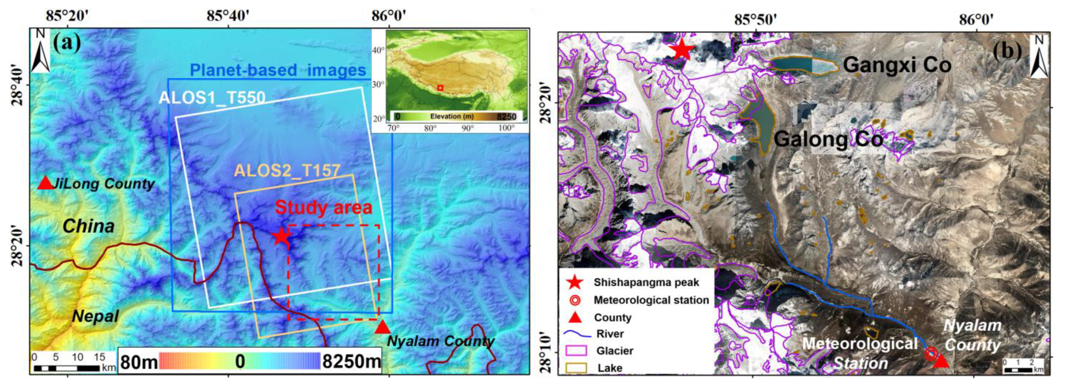
The study focused on two glacial lakes, Galong Co (28.32°N, 85.85°E) and Gangxi Co (28.35°N, 85.88°E), situated on the southeastern slope of Shishapangma (8021 m) in the central Chinese Himalaya. These lakes are moraine-dammed and located at elevations of 5220 m and 5089 m above sea level, respectively. They serve as the headwaters of the Poiqu River and are recognized as the largest and most hazardous lakes in the Poiqu River basin [31,32,33,34,35,36]. The drainage area of the basin is approximately 2160 km2 [32,38].
The southern slope of the Shishapangma region receives a higher amount of precipitation compared to the northern slope. Based on observations at Nyalam station, located at an altitude of 3810 m~17 km from Galong Co, the mean annual temperature was recorded as 3.7 °C, while the mean annual precipitation amounted to 650.7 mm during 1967–2012 [38]. Approximately 60% of the annual precipitation in the study area occurs during the summer monsoon, specifically between July and September [34]. Among these months, September experiences the highest peak in precipitation, with an average precipitation of 87.9 mm per month. After October, precipitation levels decrease significantly, and November is the driest month, with an average of 13.0 mm of precipitation. Precipitation then gradually decreases until May, after which it begins to increase again.
Here, we chose the representative Galong Co, which poses a great threat to Nyalam town, and designed a whole flowchart for GLOF monitoring using remote sensing methods and GLOF modeling using HEC-RAS. We collected and processed multi-source remote sensing datasets in our study. Figure 1 illustrates the spatial footprints of SAR images from ALOS-1 PALSAR-1 and ALOS-2 PALSAR-2 satellites and optical images from Planet satellite.
2.1. Optical Images
Planet Labs (https://www.planet.com, accessed on 1 January 2023) collects high-resolution optical images, including RapidEye and PlanetScope datasets. RapidEye images of 5 m resolution have five electromagnetic bands: blue (400–510 nm), green (520–590 nm), red (630–680 nm), red-edged (690–730 nm), and near-infrared (760–850 nm). PlanetScope images of ~3–4 m resolution have four electromagnetic bands: blue (455–515 nm), green (500–590 nm), red (590–670 nm), and near-infrared (780–860 nm). Temporal changes in the glacial lake area from 2010 to 2020 were identified using PlanetScope and RapidEye images (Table 1). A total of eight optical images taken during 2010–2020 at 3–5 m resolution from October to December in winter were selected because they had less cloud cover, which allowed for us to map the glacial lakes. We also obtained the glacier lake area in 1990 from the inventory, archived at the National Tibetan Plateau Data Center (TPDC) (https://data.tpdc.ac.cn, accessed on 1 January 2023) [39].
2.2. SAR Data
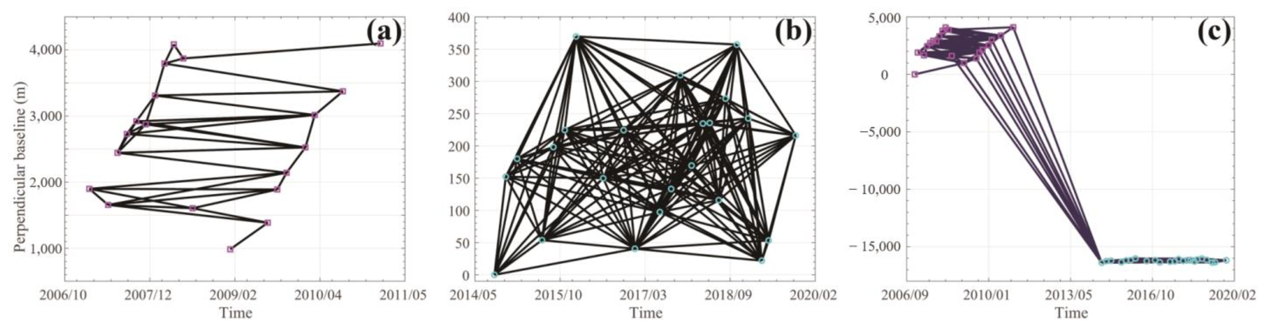
Multiple remote sensing datasets were used to obtain the deformation velocity and long-term deformation time series of the lake dam, and deformations in mother glaciers. We collected and processed spaceborne SAR images from the ALOS-1 PALSAR-1 and ALOS-2 PALSAR-2. Specifically, we utilized 20 ALOS-1 PALSAR-1 images from ascending track T550 for 2007–2011 and 23 ALOS-2 PALSAR-2 images from ascending track T157 for 2014–2020. Figure 2 shows the spatial–temporal baseline map used in the SBAS-InSAR methods.
2.3. Glacier Thickness Change Data
We examined the thickness change in mother glaciers in the study area during 1975–2000 and 2000–2016 using the datasets from the National Snow and Ice Data Center [40], https://nsidc.org/data/, accessed on 1 January 2023). In this study, the datasets used to compute glacier thickness using multi-temporal DEMs consisted of differential DEMs from KH-9 HEXAGON, which are military satellites utilized by US intelligence agencies, and ASTER, a sensor launched aboard the Terra satellite by NASA and Japan’s Ministry. Prior to the computation, individual DEMs obtained from the Shuttle Radar Topography Mission (SRTM) were registered with a spatial spacing of 30 m.
2.4. DEM Data
Data for High-Mountain Asia (HMA) at 8 m DEM, obtained from NASA Earth data (https://nsidc.org/, accessed on 20 December 2019), were utilized in this study for hydrological modeling purposes. The HMA DEM is generated by the following DigitalGlobe satellites: GeoEye-1, WorldView-1/2/3, and QuickBird-2: GeoEye-1, WorldView-1/2/3, and QuickBird-2, provided by the National Snow and Ice Data Center (https://nsidc.org). Both WorldView and GeoEye along-track data pairs have horizontal/vertical accuracies of less than 5 m, while Quickbird-2 data pairs have lower horizontal (23 m) and vertical accuracies. The relative error within a single DEM band depends on the geometry of the stereo pair and the slope of the surface, but is generally less than 1–2 m [41]. The DEM was generated using high-resolution along-track and cross-track stereoscopic images from Digital Globe satellites. The DEM covers Asian high-mountain glaciers and snowfall regions [41]. However, some areas have limited spatial coverage in the mosaic DEM products. Then, we used the 1-arcsec Shuttle Radar Topography Mission (SRTM) of 30 m to calculate the phase contributions from the topography during the InSAR processing. The SRTM data that are available on the Earth Explorer website are derived from radar measurements collected during the Shuttle Radar Topography Mission (https://earthexplorer.usgs.gov/, accessed on 1 January 2023).
2.5. Meteorological Data
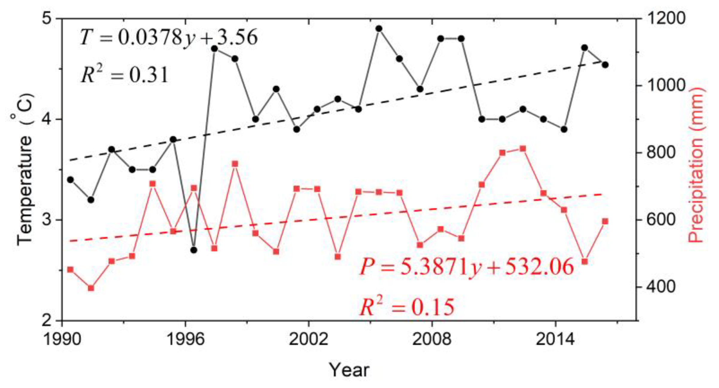
We collected mthe temperature and precipitation data at a meteorological station in Nyalam (Figure 3). During the period of 1990–2016, the annual air temperature showed an increase at a rate of 0.4 °C per decade. The annual precipitation also exhibited an increase during 1990–2016, at a rate of 53.9 mm per decade. The combination of warming temperatures and increased precipitation likely promoted glacier acceleration and lake area expansion. Table 1 summarizes the parameters of the multi-source remote sensing data used in this study.
3. Method
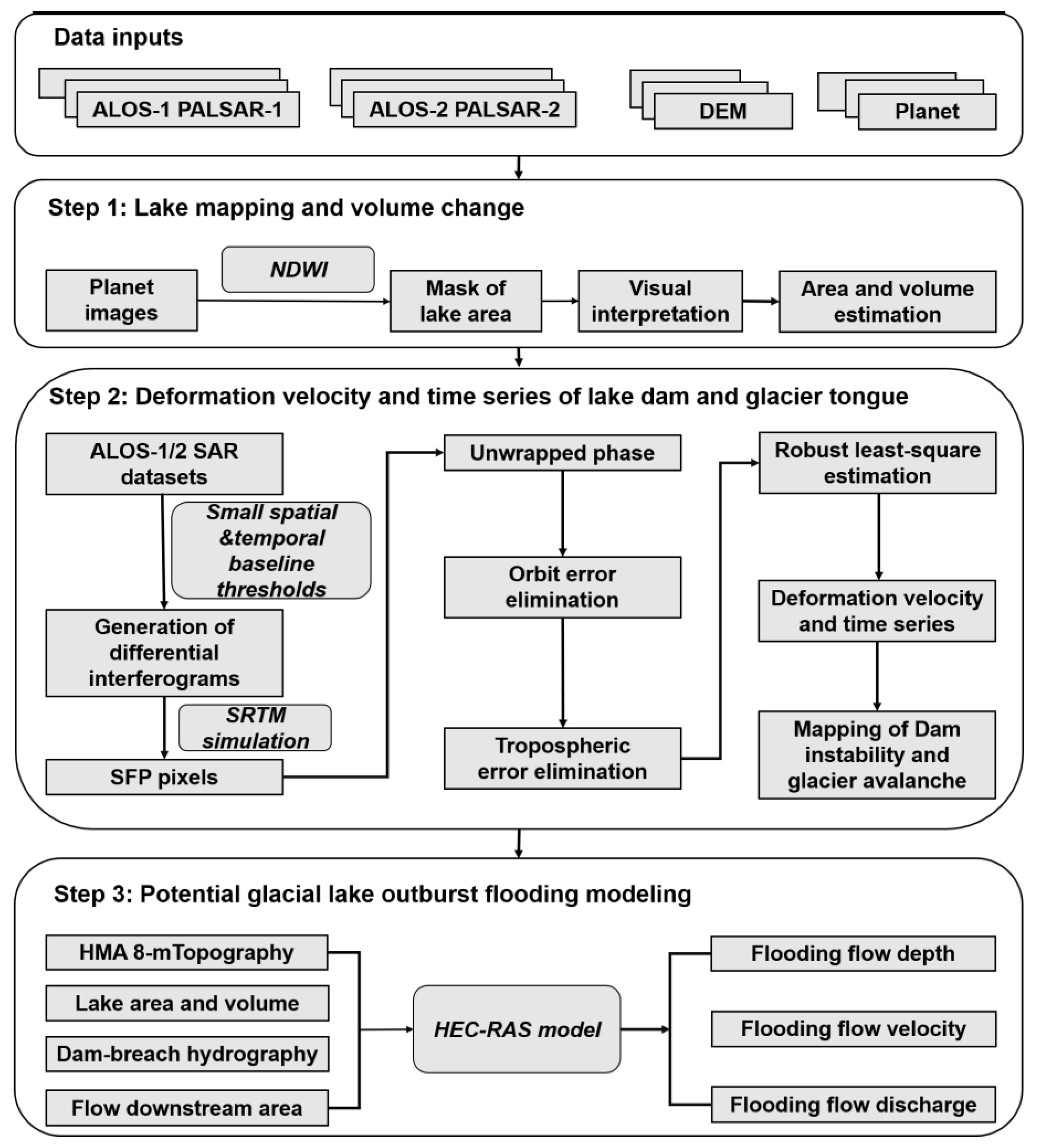
We synergized ALOS-1 PALSAR-1 and ALOS-2 PALSAR-2 data, optical Planet-based data, and the thickness change products to assess GLOF hazard using multiple remote sensing methods. Thereafter, we modeled the lake flooding processes based on HEC-RAS. The flowchart for multiple remote sensing methods and the hydrodynamic model is shown in Figure 4.
3.1. Lake Area and Volume Change Mapping with Optical Images
To monitor the area change in glacial lakes, we first marked out the glacial lake using the Normalized Difference Water Index (NDWI) based on high-resolution Planet-based images. We further calculated the volume of the glacial lake V using the empirical relationship with the lake area A in km2, with an R2 = 0.99 [13].
where V represents the lake volume (106 m3) and A represents the lake area (km2).
To estimate the uncertainty of the lake area, we employed a method using ±0.5 pixels inside and outside the delineated boundary [7,13]. This uncertainty is expressed as follows:
where is the uncertainty of a single glacial lake area; P is the perimeter; G is the spatial resolution of 5 m during 2010–2016 for RapidEye images and 3 m during 2016–2020 for Planet images.
3.2. Deformation Velocity and Time Series of Lake Dam and Glacier Tongue with SBAS-InSAR Method
The InSAR technique was employed using ALOS-1 PALSAR-1 images from 2007 to 2011 and ALOS-2 PALSAR-2 images from 2015 to 2020, allowing for an estimation of deformation velocities and time series of the lake dam and glacier tongue [10,23,24]. Details about the SAR images are provided in Table 1. SBAS-InSAR is a method that overcomes spatial and temporal decorrelation, orbital errors, and atmospheric phase artifacts by utilizing a series of SAR images [42,43]. We used the Standford Method of Persistent Scatterers (StaMPS) for processing SBAS-InSAR [42]. To further analyze the slowly varying filtered phase pixels (SFP), two processing steps were undertaken, including three-dimensional phase unwrapping and deformation-phase solution. The atmospheric artifacts, baseline errors, tropospheric artifacts, and phase ramps were estimated and reduced via temporal high-pass filtering and spatial low-pass filtering. The time series phases were then inverted using a least-squares approach [42].
3.3. GLOF Modeling with HEC-RAS
HEC-RAS is a widely used two-dimensional hydraulic model. HEC-RAS offers a range of features and capabilities that enable users to analyze and model complex hydraulic scenarios [29,35]. By solving the full 2D Saint Venant equations or the 2D Diffusion Wave equations, HEC-RAS provides a robust framework for modeling and analyzing hydraulic phenomena. The model setup for HEC-RAS involves several important steps to accurately represent the hydraulic system being analyzed. These steps typically include terrain model creation, upstream and downstream boundary conditions, Manning roughness values, and spatial domain definition.
To model the GLOF of Galong Co, we utilized an HMA DEM with an 8 m spatial resolution. The geometry data include the lake, the dam, and the flow area. The lake area and volume were obtained from optical images. The initial dam geometry, such as dam breaching depth and breaching width, was estimated by Equations (3)–(5). The flow area covered the lake and Nyalam, with computational boundaries extending 500 m on either side of the central line of the flow channel. This flow area was divided into equal 30 × 30 m grids to perform unsteady flow computations for each scenario, allowing for us to analyze breach hydrographs in detail. We set the Manning roughness coefficients to 0.03 for the downstream channel. This value is determined in terms of the land cover and vegetation and is recommended to be 0.025–0.033, where there is no vegetation in the channel [28,29,38]. We utilized the full momentum equation to model the flow dynamics. Hydraulic computation time was set to 24 h. The mapping output interval was set to 5 min. The simulation time step was set to one second, while providing upstream and downstream boundary conditions. We estimated the dam breach hydrographs using Equations (3)–(5) as the upstream boundary conditions. For the downstream boundary conditions, we used an energy slope of 0.02 m/m to show the discrete slope at the downstream cross-section [28,31,38].
3.4. Dam Breach Hydrography
We employed empirical formulae as the simplest approach to estimating dam breach hydrographs.
The output of empirical equations typically includes dam failure time () and peak discharge (). We used Froehlich’s equations [44] due to their low uncertainty compared with other approaches [45].
where is the dam breach height (in m); is the volume above of the lake (in m3); is the depth of water above the breach invert at the time of failure (in m); is the time taken for the breach to form (in h); is the peak discharge (in m3/s). In previous studies of Galong Co modeling [38], the breach depth was typically determined based on the moraine geometry. However, in our study, we utilized an empirical relationship derived from a comprehensive dataset comprising 182 cases of earth and dam failure incidents to estimate the dam breaching depth according to the method of Xu and Zhang [46]. This formula, which incorporates fewer physical parameters, is well-suited for situations where the type and failure mode of the dam are unknown [46]. It considers the degree of erosion of the dam and exhibits minimal uncertainty. The proposed breaching depth prediction shows better accuracy compared with the existing models (R2 = 0.82). The breach depth is related to the dam height, as shown in Equation (4):
in which = 1.072, 0.986, and 0.858 represent high, medium and low dam erodibility, respectively. is the dam height, and = 15 m [46]. The potential flood volume (PFV) can be assessed using the concept introduced by Fujita et al. [47]
where is the breach height (in m), is the mean depth of the lake (in m), and A is the lake area (in m2).
In the case of Galong Co, the dam height is 95 m, calculated using the high-resolution HMA DEM and the previous studies [38]. The mean depth is 86 m; the mean area is 5.46 km2 [17]. The dam breach depths using Equation (4), with high, medium, and low erosion, are ~87 m (D1), ~78 m (D2), and ~66 m (D3), respectively. Then, the related flood volumes obtained using Equation (5) are ~469 Mm3 (V1), ~426 Mm3 (V2), and ~360 Mm3 (V3). By using different breaching depths and release volumes for GLOF modeling, GLOF simulations offer the possibility of obtaining a more comprehensive understanding of GLOF dynamic routing.
3.5. GLOF Triggering Modeling and Sensitivity Analysis
We conducted GLOF modeling for different breach depths, considering high, moderate, and low dam erodibility scenarios. We evaluated the GLOF process by simulating three scenarios based on changes in breach depth and the related release volume. Here, we considered three scenarios based on different breach depths and corresponding release volumes: a high breach depth with a large-magnitude release volume (D1-V1); a medium breach depth with a moderate-magnitude release volume (D2-V2); a low breach depth with a low-magnitude release volume (D3-V3). Each scenario represents a specific combination of breach depth and release volume.
We simulated the resulting GLOF processes for the three scenarios by varying input dam breach hydrographs and release volume and evaluated the GLOF process chains using HEC-RAS. The obtained outflow hydrographs for each scenario are dynamically routed using HEC-RAS (2D) to assess the flow hydraulics downstream. Thereafter, a sensitivity analysis was performed using these full-range GLOF scenarios.
4. Results and Discussions
4.1. Gangxi Co and Galong Co Expansion
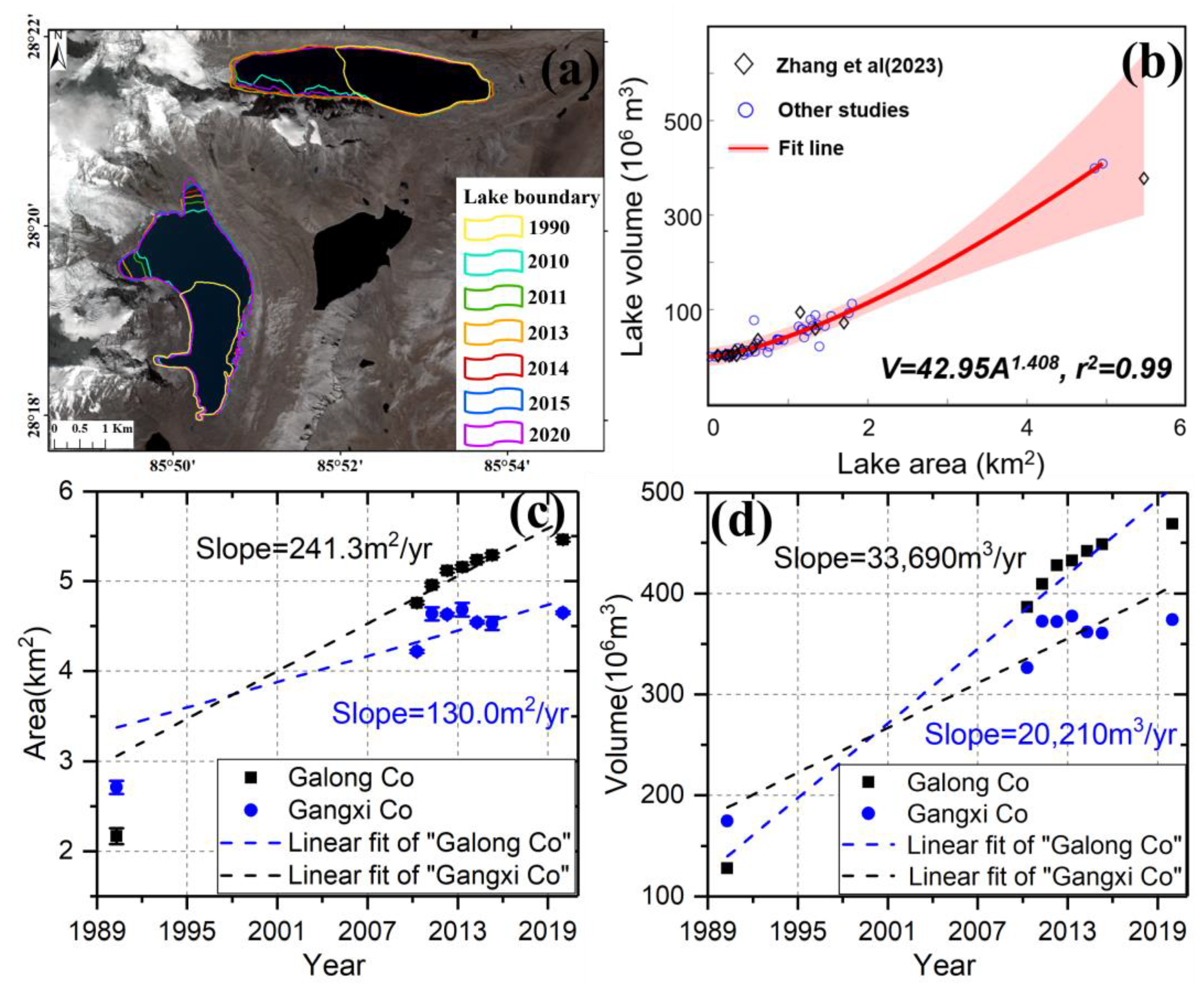
We retrieved the evolution of Gangxi Co and Galong Co from 2010 to 2020 using optical Planet-based images. Figure 5 shows the evident expansion of the lake area and its volume. According to the inventory from TPDC [38], the area of Gangxi Co and Galong Co in 1990 were 2.71 ± 0.07 km2 and 2.17 ± 0.09 km2, respectively. By the winter of 2010, the Gangxi Co and Galong Co had expanded to 4.22 ± 0.03 km2 and 4.76 ± 0.03 km2, respectively, about twice that in 1990. In 2020, Gangxi Co and Galong Co continued to expand, reaching 4.65 ± 0.02 km2 and 5.46 ± 0.02 km2, respectively. We found that Ganglo Co and Gangxi Co increased 241.3 ± 0.03 m2/yr and 130.0 ± 0.03 m2/yr by area, respectively (Figure 5c). The volume of the two lakes was estimated using an empirical area–volume relationship proposed by Zhang et al. [13], as shown in Figure 5b. During 1990–2020, the lake water volume of Galong Co increased from 127.6 × 10⁶ m3/yr to 469 × 106 m3/yr, at a rate of 0.03 × 10⁶ m3/yr. The lake volume of Gangxi Co increased from 174.7 × 10⁶ m3/yr to 373.9 × 10⁶ m3/yr, at a rate of 0.02 × 10⁶ m3/yr (Figure 5d).
Gangxi Co expanded to the west while Galong Co expanded northwesterly to the source of the glacier meltwater. These two glacial lakes follow the expanding behaviors of end-moraine dammed lakes where the moraine is connected to the mother glaciers. Therefore, the new land created by the glacier retreating allows for lake expansion. Changes in lake area and volume suggest that proglacial lakes accelerate the glacier’s retreating and thinning.
4.2. Deformation Velocity and Time Series of Glacial Lake Dam
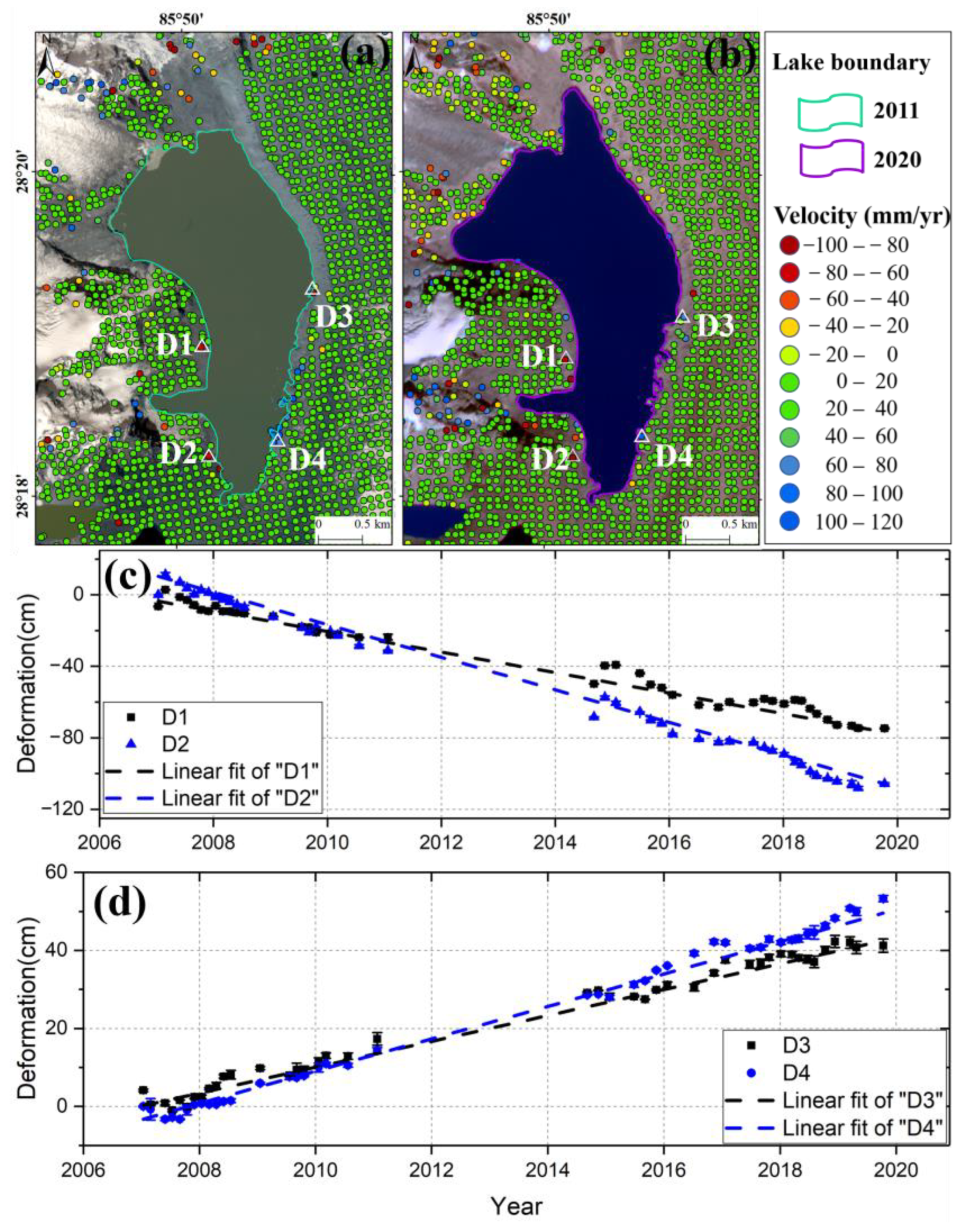
Lake dam deformation is a direct indicator of dam instability [47]. About 775,117 and 552,120 coherent pixels of ALOS-1 and ALOS-2 data, respectively, were selected in this study area. We monitored the LOS velocity of the lake dam by focusing on measurement points around the Galong Co, as shown in Figure 6. The LOS deformation rates in Figure 6a,b show that the Galong Co dam and the glacier tongues deformed during 2007–2020, while the surrounding land remained stable. Due to the different imaging geometries and timing of ALOS-1 and ALOS-2 datasets, the deformations observed on different distribution measurement points presented different patterns. However, the deformation velocity of 220 mm/yr during all periods can imply the presence of rapid changes in the shapes or behavior of dam structures.
The cumulative deformation time series is another important parameter of interest in our study. To obtain a deeper understanding of the kinematic behavior of the lake dam, we plotted the deformation time series for four selected dam points (D1–D4 in Figure 6a,b). Due to the different distribution of the measurement points, we selected D1 and D3, which are located in different positions. Moreover, we assessed the accuracy of the deformation time series using root mean square error around these selected points, represented by the error bar in Figure 6. D1 and D2 were located in the west moraine around the lake dam, while D3 and D4 were located in the east moraine around the lake dam. The downslope from the west lateral moraine at D1 and D2 is the most active area, with a cumulative deformation of 74.8 ± 0.5 cm and 105.7 ± 0.6 cm around the lake dam, respectively. The cumulative deformation measurements of D3 and D4 situated on the east moraine were 41.2 ± 0.2 cm and 53.3 ± 0.8 cm during 2007–2020. Permafrost and ground ice in the lake dam structure likely contributed to the deformation behaviors of the lake dams. Deformation observations around the lake dam of Galong Co play a primary role in ensuring the safety of the outlet structure.
4.3. The Source Zones of Glacier Mass Movements and Thickness Change
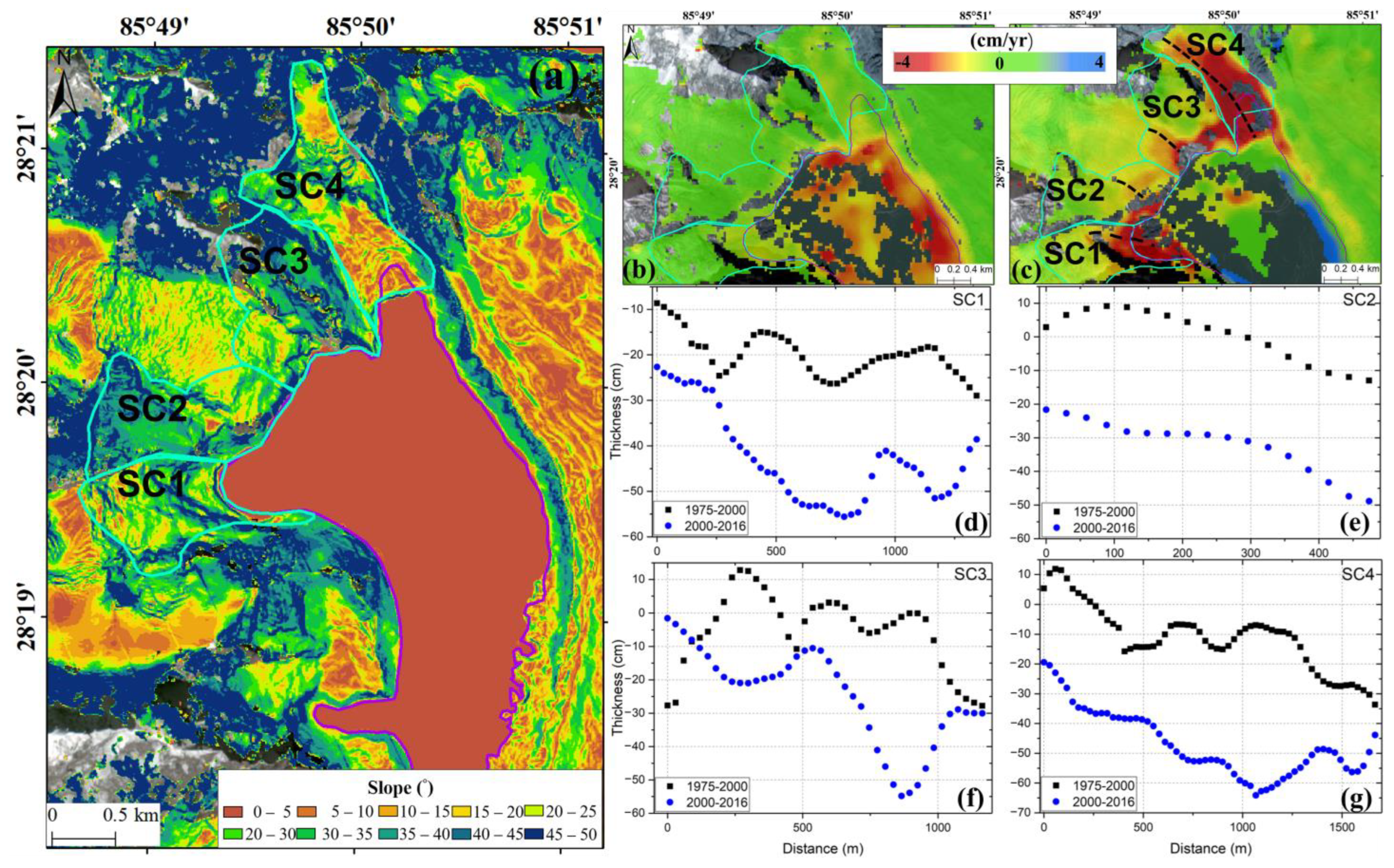
Glacier avalanches or landslides occurring in glaciated terrains have a direct impact on high-altitude lakes, generating massive displacement waves and leading to GLOF events. In our study, we identified slopes with steep angles (greater than 20°) using DEM analysis based on 8 m HMA DEM and Google Earth images. The slope values are based on ice/rock avalanche events reported within an extensive global catalog of events contained in the literature [17,18,36]. These unstable ice masses, situated at the glacier headwall, have a high potential to reach the lake (Figure 7a). Then, we compared the glacier thickness changes during the two periods based on thickness products.
The results show that the glacier–lake interface experienced a higher rate of thinning during 2000–2016 compared to that during 1975–2000 (Figure 7b,c). The four identified sources show the glacier thinning and mass loss. We analyzed the thickness changes in four profiles of their source zones, as shown in Figure 7d–g. The thickness changes in the four profiles show that the glacier source zones experienced a clear thinning trend from 2000 to 2016. The maximum thinning that occurred during 2000–2016 in source 1 (SC1), source 2 (SC2), source 3 (SC3), and source 4 (SC4) reached −56 cm, −49 cm, −55 cm and −64 cm, respectively. The acceleration of glacier thinning, and the expansion of glacial lakes, in terms of both size and depth, can potentially contribute to glacier avalanches and subsequent lake outburst flooding.
4.4. Hazard Analysis of GLOFs
Previous studies showed that GLOF can be triggered by several factors, including rapid slope movement into lakes, heavy precipitation, earthquakes, the melting of ice in the dam, the blocking of subsurface outflow tunnels, and the gradual deterioration of the dam over time [8,9,10].
Our study considered three primary factors to analyze GLOF hazards, including atmospheric, cryospheric, and geomorphic factors. Table 2 displays the detailed factors and related methods and sources. Increased air temperatures across the study area will lead to higher lake water temperatures, causing enhanced melt rates that will intensify subaqueous mass reduction until the glacier separates from the lake [13]. The increasing precipitation can lead to high lake-water levels, which may cause high-magnitude events if a GLOF occurs. The expansion in lake area and volume increased the GLOF risk as a result of the high potential flood magnitude. Sattar et al. [29] indicated that lowering the glacial lake considerably reduces the downstream exposure. The changes in glacier thinning can reveal the glacier mass loss. The glacier thinning and mass loss that occurred at the glacier–lake interface will drive the glacier mass movement into the lake and the resulting GLOF. Thereafter, we identified the four avalanche sources based on the topographic slope (>20) and instability (Figure 8).
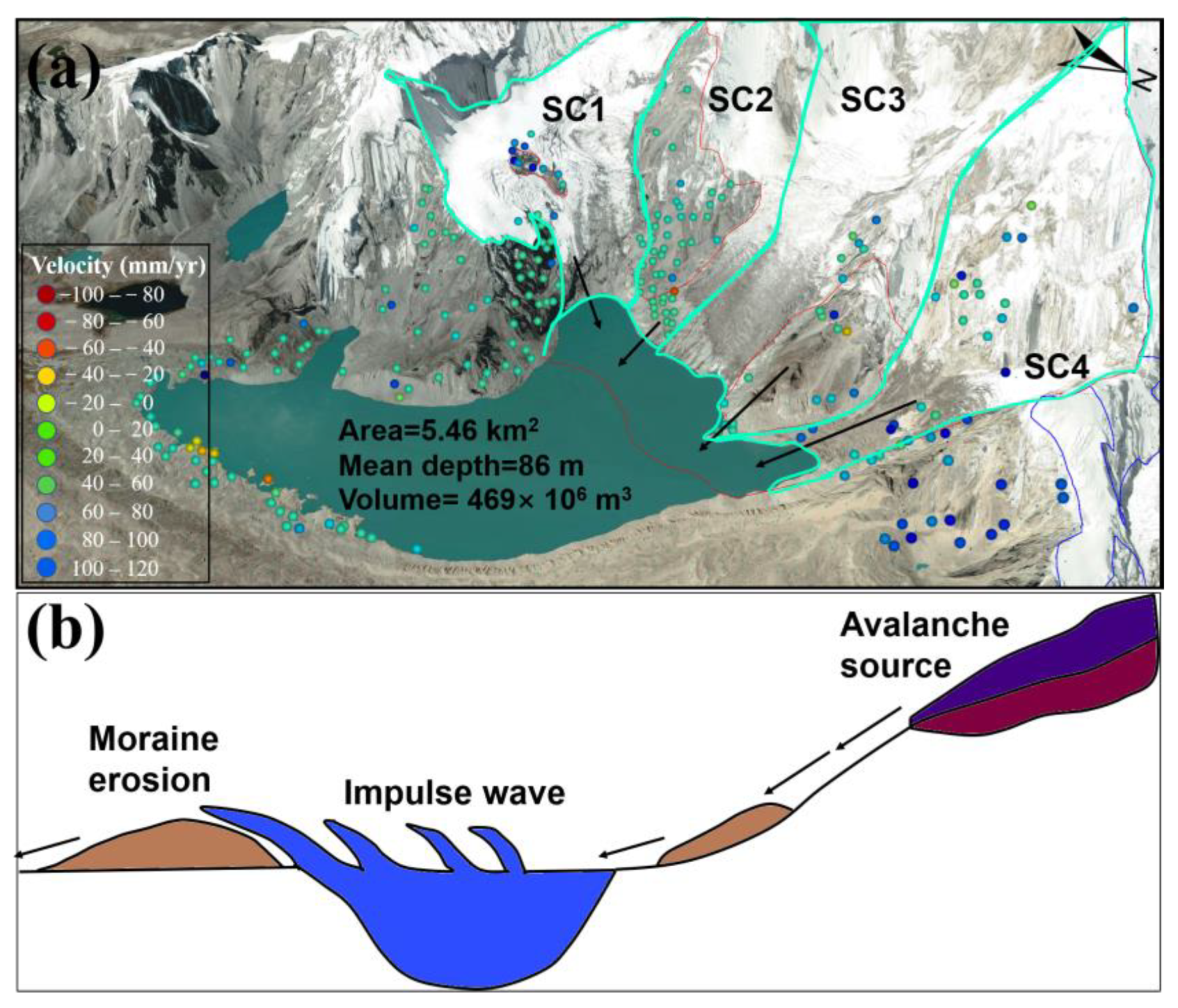
Figure 8a displays the four potential avalanche zones that could contribute to Galong Co outburst. Steep ice cliffs are located on high mountain slopes around Galong Co. The deformation rate in these mountain slopes shows the downslope movement with a maximum measurable velocity of 220 mm/yr. We need to note that the SBAS-InSAR method may not work when the glacier surface features are extensively modified during rapid movement. The maximum volume of glacier/ice avalanches on these four potential avalanche zones were in the range 0.1–1 × 10⁶ m3 for Galong Co [17]. For geomorphic factors, we analyzed the dam type, downstream slope of the dam, and dam stability. The construction of dam structures involves various materials, such as ice, moraine, or bedrock [46]. In the case of Galong Co, the construction of the dam involves moraine and ice. The downstream slope in the lake dam is 10°. Moreover, the deformation velocity and time series of the dam were obtained based on the SBAS-InSAR method. The dam experienced variable movement rates from 2007 to 2020, especially at the downstream D2 and D4 points. The monitoring of long-term deformation around the lake dam provides us with essential dam structure health issues. These studies provide a new understanding of the hazard chain analysis of Galong Co using multiple remote sensing methods.
Nonetheless, the substantial water volume within the lake and the gradual downstream slope of the dam significantly reduce the likelihood of a catastrophic failure resulting from gradual process piping [17]. Therefore, we considered that high-magnitude triggering factors, such as glacier avalanches, are likely to initiate a GLOF. Figure 8b shows the avalanche mass movement into the lake and the GLOF hazard chain. Mass movements resulting from glacier avalanches or calving events enter a lake, giving rise to displacement waves resembling tsunamis. This can lead to the overtopping of the moraine dam and potentially initiate erosion at the crest of the dam.
4.5. GLOF Modeling
The potential hazards originating from Galong Co can have catastrophic outcomes owing to the large volume of the lake. We evaluated the impact of Galong Co on Nyalam County using HEC-RAS modeling.
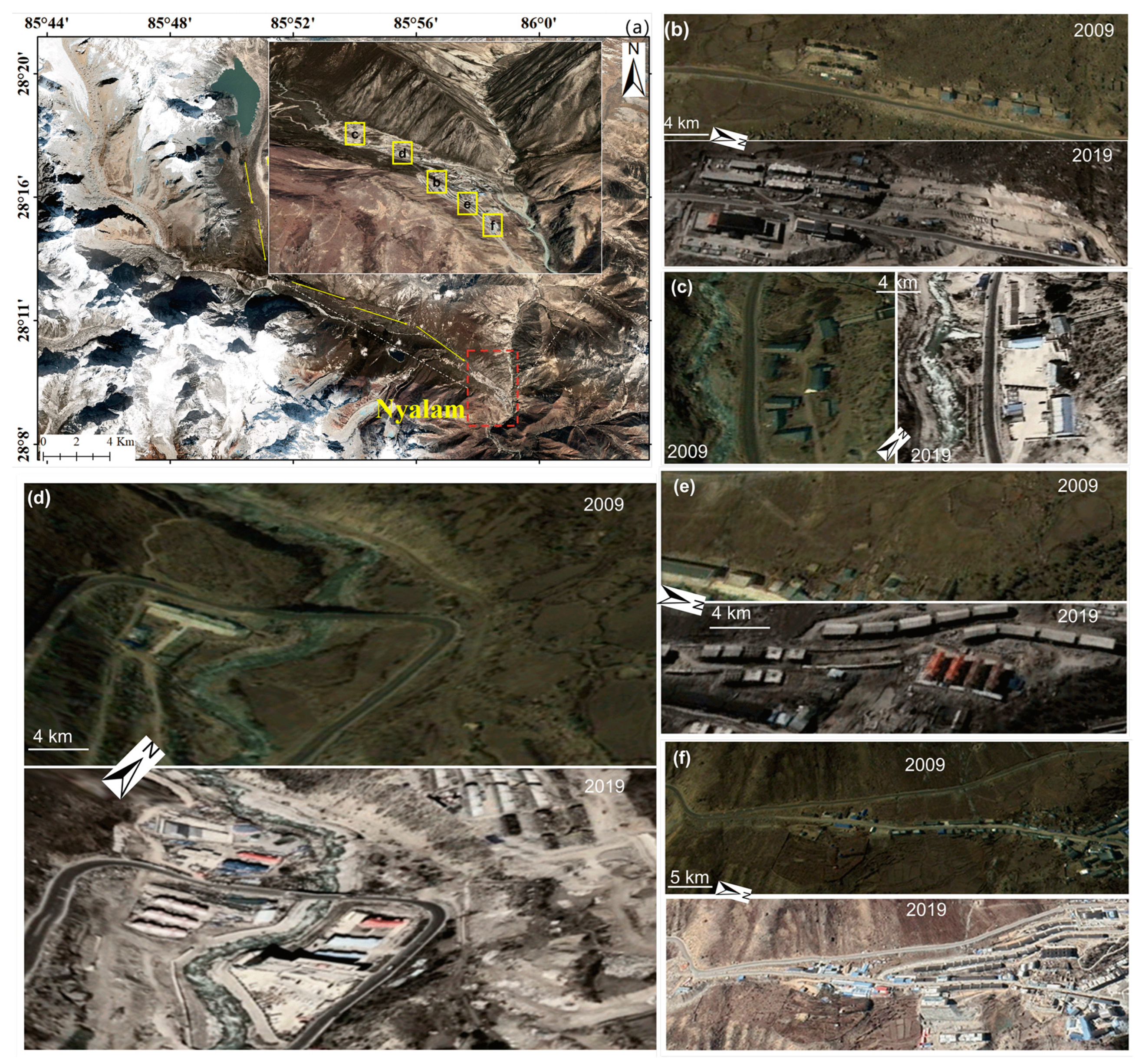
Figure 9 shows the expansion and development of infrastructure in the study site from 2009 to 2019. Figure 9a shows the flooding direction and downstream environment of Galong Co. We extracted five sites from Nyalam Town, as shown in Figure 9b–f. These buildings were recently constructed around roads and riverbanks, which are exposed to flooding paths in the event of GLOF. The study area reveals a clear trend of expansion, not only in the size of lakes but also in the growth of infrastructure within GLOF-exposed regions. The increase in population and excessive construction of infrastructure highlights the urgent need for a GLOF hazard assessment and flooding model.
We evaluated the GLOF hazard process in these three different scenarios, considering the varied magnitudes of release volume and dam-breach parameters (Table 3). Three different scenarios include: the breaching depth of ~87 m (D1) and the related flood volumes of ~469 Mm3 (V1); the breaching depth of ~78 m (D2) and the related flood volumes of ~426 Mm3 (V2); the breaching depth of ~66 m (D3) and the related flood volumes of ~360 Mm3 (V3). To conduct a comprehensive analysis of dam breach and downstream propagation, we employed scenario-based modeling (Table 3). In the high-erosion dam breach and large-magnitude release volume scenario (D1-V1), a GLOF results in a breach width of 229 m. The breach formation takes 1.80 h. The predicted depth of the medium-erosion dam breach with modern-magnitude release volume (D2-V2) causes a breach width of 224 m and a breach formation time of 1.89 h. The predicted depth of the low-erosion dam breach with low-magnitude release volume (D3-V3) produces a breach width of 214 m and a breach formation time of 2.01 h. The peak discharge for the three breaching scenarios ranges from 36,615.1 to 55,742.8 m3/s.
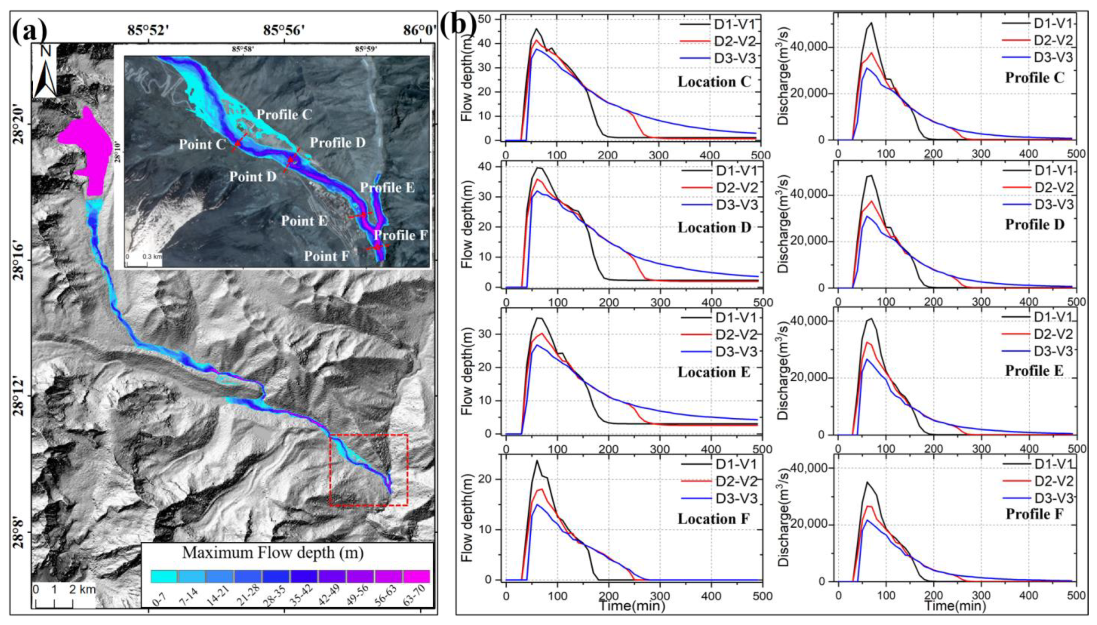
We analyzed the inundation impact downstream at Nyalam (Figure 10, Table 4). Table 4 evaluates the peak discharge and the maximum flow depth of the GLOF at downstream locations C-F (Figure 10). A higher breaching depth and larger release volume result in a larger flow depth and discharge. The peak discharge and the maximum flow depth of the GLOF decrease at all four locations as the breach depth gradually decreases.
Figure 10a illustrates the maximum flow depth for the large-magnitude release volume (V1) using a breaching depth of 87 m (D1). Subsequently, we analyzed the GLOF routing flow depth and discharge at different positions in Nyalam under three scenarios, as shown in Figure 10b.
For the scenario with a high breaching depth and large-magnitude release volume (D1-V1), the maximum flow depth is ~46.1 m, and the peak discharge is ~50,625.1 m3/s at position C. At site D, the maximum flow depth and discharge decrease to ~40.0 m and 48,454.9 m3/s, respectively. The maximum modeled flow depth is ~34.8 m, and the peak GLOF discharge is ~40,923.3 m3/s at position E. The GLOF flow depth reduces to ~23.8 m, and the outflow peak is ~35,097.8 m3/s at position F.
For the moderate-magnitude release volume (V2), the medium-erosion breaching depth (D2) results in a maximum flow depth of ~41.4 m and a peak discharge of ~37,697.2 m3/s at position C. At position D, the GLOF peak discharge is ~37,483.7 m3/s, with the flow depth reaching up to ~36.0 m. The predicted GLOF peak discharge at site E reaches ~32,587.2 m3/s, with the flow depth reaching ~30.3 m. At position F, the scenario (D2-V2) results in a GLOF peak of ~26,667.2 m3/s, with the flow depth lowering to ~18.0 m.
For the low-erosion dam breaching depth and low-magnitude release volume (D3-V3), the maximum flow depth is ~37.7 m, and the GLOF peak discharge reaches ~31,015.4 m3/s at position C. In this scenario, the routed hydrographs at site D show that the maximum depth of the GLOF reaches ~32.0 m, and the peak discharge is ~30,963.5 m3/s. The maximum flow depth and peak discharge at position E are reduced to ~26.8 m and 26,658.7 m3/s, respectively. For the GLOF routing at site F, the depth lowers to ~15.0 m, and the peak discharge decreases to ~21,748.6 m3/s.
In our GLOF modeling, we consider a range of potential avalanches and breaching depths, which are important for hazard mitigation and preparedness. Although the release volume is high and the likelihood is low, it is important to consider the implementation of early warning systems, and risk reduction measures, including worst-case scenarios.
4.6. Uncertainties and Future Direction
In this study, we examine GLOF scenarios that incorporate the possibility of avalanche-induced impacts on the lake. Under all current scenarios, the Nyalam region is susceptible to GLOFs of high intensity (with flow depth greater than one meter). However, uncertainties arise from the definition of the initial mass movement scenario, lake bottom topography and volume, and the parameters used in the model. To identify avalanche source zones, we use topographic slope and deformation data, as well as information from previous studies [17]. By varying the release volume and dam hydrography for three different scenarios, we examine how changes in these factors affect flow depth and discharge. Simulating intricate GLOF processes in high-mountain environments presents a non-standard challenge, and parameter sets obtained from a limited number of GLOF simulations using an evolving simulation framework like HEC-RAS [26] introduce substantial uncertainties that are often challenging to quantify. Allen et al. [36] achieved a flow depth of 37 m and a peak discharge of 42,917 m3/s at Nyalam in the full-release volume scenario, which is consistent by orders of magnitude with the D1-V1 scenario in our study. Our study reveals that the GLOF process can vary based on the magnitude, characteristics, and location of the initial mass movement, and remains highly uncertain due to alterations in the lake and its surroundings. The current GLOF model that we developed serves as a foundation for conducting disaster risk reduction analysis by modifying the lake volume and dam height.
In the downstream reach to the border, where there are few buildings along the riverbank, the main threat is the 38 km long cross-country highway [36]. Although the flood we modeled did not extend to the border due to the limited coverage of the required high-resolution HMA DEM, previous studies have shown that the proportion affected by high-intensity flooding is 40% in Nepal, and there are potential property losses reaching over USD 197 million in downstream communities of Nepal from this GLOF [31,33,36]. Glacial lake flooding from Galong Co poses a significant risk to Nepalese communities, hydropower stations, and other infrastructure along the Bhote Koshi River [36]. Hence, collaborative efforts among nations are needed to mitigate and manage transboundary risks from the GLOF hazard. The continuous monitoring of lake dams and glacier avalanches is crucial to ensuring their structural integrity. InSAR technology is favored for its ability to monitor slope movements and the instability of moraine dams [21,27]. For future work, we recommend regular and continuous monitoring of the lake and its surrounding areas.
5. Conclusions
Owing to the increasing trend in global warming, glaciers in the Shishapangma area have experienced rapid retreat and thinning, thereby resulting in the expansion of glacial lakes and an increase in outburst hazards. In this study, we conducted a comprehensive analysis of Galong Co using various remote-sensing techniques and numerical models. First, the area and volume of Galong Co were calculated using optical Planet-based images, which showed an increase in the rate of area and volume of 241.3 m2/yr and 0.03 × 10⁶ m3/yr, respectively. Second, we used two SAR datasets, ALOS-1 PALSAR-1 and ALOS-2 PALSAR-2, to derive long-term deformation time series of the lake dam using SBAS-InSAR method. We monitored the instability of the lake dam that occurred on the lateral moraine from 2007 to 2020. The cumulative maximum deformation reaches up to 105.7 ± 0.6 cm on the west moraine. Third, the thickness change in the mother glaciers suggested that thinning occurred at the glacier–lake interface, which caused glacier mass loss and lake area expansion. Finally, we identified potential avalanche sources by analyzing topographic slopes greater than 20°, glacier thinning trends, and measurable deformations on the glacier surface. In addition, we conducted a flooding modeling of Galong Co to evaluate the flow depth, flow discharge and time-series process, considering different release volumes and dam breach hydrography. Our hydrodynamic modeling analysis indicated that the Nyalam region is exposed to high-intensity GLOFs in all scenarios, with larger breaching depth and release volumes causing greater flow depth and peak discharge. As the breach depth gradually decreases, the peak discharge and maximum flow depth of the GLOF decrease downstream.
The findings of the present study demonstrate that multiple remote sensing methods are effective approaches for detecting lake dam instability and glacier movement in mountainous regions. The advancement of SAR imagery archives and techniques has ushered in a new era in glacial lake identification and monitoring, significantly enhancing our comprehension of lake outburst hazards.
Author Contributions
Conceptualization, L.Y. and Z.L.; methodology, L.Y., Z.L. and C.O.; software, L.Y.; validation, L.Y., Z.L. and C.O.; investigation, L.Y.; writing—original draft preparation, L.Y.; writing—review and editing, Z.L., C.O. and X.H.; visualization, L.Y. and X.H.; supervision, C.Z. and Q.Z; funding acquisition, C.O., C.Z. and Q.Z. All authors have read and agreed to the published version of the manuscript.
Funding
This research was supported by the National Key R&D Program of China (Grant no. 2022YFC3004302), Natural Science Foundation of China (Grant no. 41929001, 4192900003), and the Fundamental Research Funds for the Central University (Grant No. 300203211263).
Data Availability Statement
The Planet and RapidEye datasets are available from https://planet.com (accessed on 1 January 2023). The SAR data are available from https://search.asf.alaska.edu/#/ (accessed on 1 January 2023). The DEM data are available from https://earthexplorer.usgs.gov/ (accessed on 1 January 2023). StaMPS can be downloaded from http://homepages.see.leeds.ac.uk/~earahoo/stamps (accessed on 1 January 2023) and the code can be downloaded from GitHub at httpe://github.com/dbekaert/stamps (accessed on 1 January 2023).
Acknowledgments
The authors thank Planet Labs for Planet and RapidEye datasets, Japan Aerospace Exploration Agency (JAXA) and European Space Agency (ESA) for ALOS-1 PALSAR-1 and ALOS-2 PALSAR-2 data, and Qinghai-Tibet Plateau ground monitoring station for metrological data. We also thank the editor and anonymous reviewers for their helpful comments and suggestions.
Conflicts of Interest
The authors declare no conflict of interest.
References
- Gardner, A.S.; Moholdt, G.; Cogley, J.G.; Wouters, B.; Arendt, A.A.; Wahr, J.; Berthier, E.; Hock, R.; Pfeffer, W.T.; Kaser, G. A reconciled estimate of glacier contributions to sea level rise: 2003 to 2009. Science 2013, 340, 852–857. [Google Scholar] [CrossRef] [PubMed]
- Kääb, A.; Berthier, E.; Nuth, C.; Gardelle, J.; Arnaud, Y. Contrasting patterns of early twenty-first-century glacier mass change in the Himalayas. Nature 2012, 488, 495–498. [Google Scholar] [CrossRef] [PubMed]
- King, O.; Quincey, D.J.; Carrivick, J.L.; Rowan, A.V. Spatial variability in mass loss of glaciers in the Everest region, central Himalayas, between 2000 and 2015. Cryosphere 2017, 11, 407–426. [Google Scholar] [CrossRef]
- Richardson, S.D.; Reynolds, J.M. An overview of glacial hazards in the Himalayas. Quat. Int. 2000, 65, 31–47. [Google Scholar] [CrossRef]
- Song, C.; Huang, B.; Ke, L.; Richards, K.S. Remote sensing of alpine lake water environment changes on the Tibetan Plateau and surroundings: A review. ISPRS J. Photogramm. Remote Sens. 2014, 92, 26–37. [Google Scholar] [CrossRef]
- Wang, W.; Yao, T.; Gao, Y.; Yang, X.; Kattel, D.B. A first-order method to identify potentially dangerous glacial lakes in a region of the southeastern Tibetan Plateau. Mt. Res. Dev. 2011, 31, 122–130. [Google Scholar] [CrossRef]
- Fujita, K.; Sakai, A.; Nuimura, T.; Yamaguchi, S.; Sharma, R.R. Recent changes in Imja Glacial Lake and its damming moraine in the Nepal Himalaya revealed by in situ surveys and multi-temporal ASTER imagery. Environ. Res. Lett. 2009, 4, 045205. [Google Scholar] [CrossRef]
- Emmer, A. Glacier retreat and glacial lake outburst floods (GLOFs). In Oxford Research Encyclopedia of Natural Hazard Science; Oxford University Press: Oxford, UK, 2017. [Google Scholar]
- Emmer, A.; Cochachin, A. The causes and mechanisms of moraine-dammed lake failures in the Cordillera Blanca, North American Cordillera, and Himalayas. AUC GEOGRAPHICA 2013, 48, 5–15. [Google Scholar] [CrossRef]
- Yang, L.; Lu, Z.; Zhao, C.; Kim, J.; Yang, C.; Wang, B.; Liu, X.; Wang, Z. Analyzing the triggering factors of glacial lake outburst floods with SAR and optical images: A case study in Jinweng Co, Tibet, China. Landslides 2022, 19, 855–864. [Google Scholar] [CrossRef]
- Huggel, C.; Zgraggen-Oswald, S.; Haeberli, W.; Kääb, A.; Polkvoj, A.; Galushkin, I.; Evans, S. The 2002 rock/ice avalanche at Kolka/Karmadon, Russian Caucasus: Assessment of extraordinary avalanche formation and mobility, and application of QuickBird satellite imagery. Nat. Hazard. Earth Syst. Sci. 2005, 5, 173–187. [Google Scholar] [CrossRef]
- Shugar, D.H.; Jacquemart, M.; Shean, D.; Bhushan, S.; Upadhyay, K.; Sattar, A.; Schwanghart, W.; McBride, S.; De Vries, M.V.W.; Mergili, M. A massive rock and ice avalanche caused the 2021 disaster at Chamoli, Indian Himalaya. Science 2021, 373, 300–306. [Google Scholar] [CrossRef] [PubMed]
- Zhang, G.; Bolch, T.; Yao, T.; Rounce, D.R.; Chen, W.; Veh, G.; King, O.; Allen, S.K.; Wang, M.; Wang, W. Underestimated mass loss from lake-terminating glaciers in the greater Himalaya. Nat. Geosci. 2023, 16, 333–338. [Google Scholar] [CrossRef]
- Wang, F.; Harindintwali, J.D.; Wei, K.; Shan, Y.; Mi, Z.; Costello, M.J.; Grunwald, S.; Feng, Z.; Wang, F.; Guo, Y. Climate change: Strategies for mitigation and adaptation. Innov. Geosci. 2023, 1, 100015. [Google Scholar] [CrossRef]
- Wei, K.; Ouyang, C.; Duan, H.; Li, Y.; Chen, M.; Ma, J.; An, H.; Zhou, S. Reflections on the catastrophic 2020 Yangtze River Basin flooding in southern China. Innovation 2020, 1, 100038. [Google Scholar] [CrossRef]
- Li, D.; Shangguan, D.; Wang, X.; Ding, Y.; Su, P.; Liu, R.; Wang, M. Expansion and hazard risk assessment of glacial lake Jialong Co in the central Himalayas by using an unmanned surface vessel and remote sensing. Sci. Total Environ. 2021, 784, 147249. [Google Scholar] [CrossRef]
- Allen, S.K.; Zhang, G.; Wang, W.; Yao, T.; Bolch, T. Potentially dangerous glacial lakes across the Tibetan Plateau revealed using a large-scale automated assessment approach. Sci. Bull. 2019, 64, 435–445. [Google Scholar] [CrossRef]
- Wang, S.; Che, Y.; Xinggang, M. Integrated risk assessment of glacier lake outburst flood (GLOF) disaster over the Qinghai–Tibetan Plateau (QTP). Landslides 2020, 17, 2849–2863. [Google Scholar] [CrossRef]
- AWAL, R.; NAKAGAWA, H.; FUJITA, M.; KAWAIKE, K.; BABA, Y.; ZHANG, H. Experimental study on glacial lake outburst floods due to waves overtopping and erosion of moraine dam. Kyoto Univ. Res. Inf. Repos. B 2010, 53, 583–594. [Google Scholar]
- Cheng, S.; Zhao, W.; Yin, Z. PS-InSAR analysis of collapsed dam and extraction of flood inundation areas in laos using sentinel-1 SAR images. In Proceedings of the 2019 IEEE 4th Advanced Information Technology, Electronic and Automation Control Conference (IAEAC), Chengdu, China, 20–22 December 2019; pp. 2605–2608. [Google Scholar]
- Aswathi, J.; Kumar, R.B.; Oommen, T.; Bouali, E.; Sajinkumar, K. InSAR as a tool for monitoring hydropower projects: A review. Energy Geosci. 2022, 3, 160–171. [Google Scholar] [CrossRef]
- Wangchuk, S.; Bolch, T.; Robson, B.A. Monitoring glacial lake outburst flood susceptibility using Sentinel-1 SAR data, Google Earth Engine, and persistent scatterer interferometry. Remote Sens. Environ. 2022, 271, 112910. [Google Scholar] [CrossRef]
- Lu, Z.; Kim, J. A framework for studying hydrology-driven landslide hazards in northwestern US using satellite InSAR, precipitation and soil moisture observations: Early results and future directions. GeoHazards 2021, 2, 17–40. [Google Scholar] [CrossRef]
- Hu, X.; Wang, T.; Pierson, T.C.; Lu, Z.; Kim, J.; Cecere, T.H. Detecting seasonal landslide movement within the Cascade landslide complex (Washington) using time-series SAR imagery. Remote Sens. Environ. 2016, 187, 49–61. [Google Scholar] [CrossRef]
- Honda, K.; Nakanishi, T.; Haraguchi, M.; Mushiake, N.; Iwasaki, T.; Satoh, H.; Kobori, T.; Yamaguchi, Y. Application of exterior deformation monitoring of dams by DInSAR analysis using ALOS PALSAR. In Proceedings of the 2012 IEEE International Geoscience and Remote Sensing Symposium, Munich, Germany, 22–27 July 2012; pp. 6649–6652. [Google Scholar]
- Voege, M.; Frauenfelder, R.; Larsen, Y. Displacement monitoring at Svartevatn dam with interferometric SAR. In Proceedings of the 2012 IEEE International Geoscience and Remote Sensing Symposium, Munich, Germany, 22–27 July 2012; pp. 3895–3898. [Google Scholar]
- Darvishi, M.; Destouni, G.; Jaramillo, F. Lake Mead and Hoover dam monitoring in Nevada and Arizona states, USA using InSAR. In Proceedings of the EGU General Assembly Conference Abstracts, online, 4–8 May 2020; p. 21582. [Google Scholar]
- Sattar, A.; Goswami, A.; Kulkarni, A.V.; Emmer, A.; Haritashya, U.K.; Allen, S.; Frey, H.; Huggel, C. Future glacial lake outburst flood (GLOF) hazard of the South Lhonak Lake, Sikkim Himalaya. Geomorphology 2021, 388, 107783. [Google Scholar] [CrossRef]
- Sattar, A.; Allen, S.; Mergili, M.; Haeberli, W.; Frey, H.; Kulkarni, A.V.; Haritashya, U.K.; Huggel, C.; Goswami, A.; Ramsankaran, R. Modeling Potential Glacial Lake Outburst Flood Process Chains and Effects From Artificial Lake-Level Lowering at Gepang Gath Lake, Indian Himalaya. J. Geophys. Res. Earth Surf. 2023, 128, e2022JF006826. [Google Scholar] [CrossRef]
- Schneider, D.; Huggel, C.; Cochachin, A.; Guillén, S.; García, J. Mapping hazards from glacier lake outburst floods based on modelling of process cascades at Lake 513, Carhuaz, Peru. Adv. Geosci. 2014, 35, 145–155. [Google Scholar] [CrossRef]
- Wang, W.; Gao, Y.; Anacona, P.I.; Lei, Y.; Xiang, Y.; Zhang, G.; Li, S.; Lu, A. Integrated hazard assessment of Cirenmaco glacial lake in Zhangzangbo valley, Central Himalayas. Geomorphology 2018, 306, 292–305. [Google Scholar] [CrossRef]
- Chen, N.S.; Hu, G.S.; Deng, W.; Khanal, N.; Zhu, Y.; Han, D. On the water hazards in the trans-boundary Kosi River basin. Nat. Hazard. Earth Syst. Sci. 2013, 13, 795–808. [Google Scholar] [CrossRef]
- Cook, K.L.; Andermann, C.; Gimbert, F.; Adhikari, B.R.; Hovius, N. Glacial lake outburst floods as drivers of fluvial erosion in the Himalaya. Science 2018, 362, 53–57. [Google Scholar] [CrossRef]
- Shijin, W.; Shitai, J. Evolution and outburst risk analysis of moraine-dammed lakes in the central Chinese Himalaya. J. Earth Syst. Sci. 2015, 124, 567–576. [Google Scholar] [CrossRef]
- Qi, M.; Liu, S.; Gao, Y. Zhangmu and Gyirong ports under the threat of glacial lake outburst flood. Sci. Cold Arid. Reg. 2020, 12, 461–476. [Google Scholar]
- Allen, S.K.; Sattar, A.; King, O.; Zhang, G.; Bhattacharya, A.; Yao, T.; Bolch, T. Glacial lake outburst flood hazard under current and future conditions: Worst-case scenarios in a transboundary Himalayan basin. Nat. Hazard. Earth Syst. Sci. 2022, 22, 3765–3785. [Google Scholar] [CrossRef]
- Qi, M.; Liu, S.; Wu, K.; Zhu, Y.; Xie, F.; Jin, H.; Gao, Y.; Yao, X. Improving the accuracy of glacial lake volume estimation: A case study in the Poiqu basin, central Himalayas. J. Hydrol. 2022, 610, 127973. [Google Scholar] [CrossRef]
- Zhang, T.; Wang, W.; Gao, T.; An, B. Simulation and assessment of future glacial lake outburst floods in the Poiqu River Basin, Central Himalayas. Water 2021, 13, 1376. [Google Scholar] [CrossRef]
- Zhang, G.; Yao, T.; Xie, H.; Wang, W.; Yang, W. An inventory of glacial lakes in the Third Pole region and their changes in response to global warming. Glob. Planet. Chang. 2015, 131, 148–157. [Google Scholar] [CrossRef]
- Maurer, J.; Rupper, S.; Schaefer, J. High Mountain Asia Gridded Glacier Thickness Change from Multi-Sensor DEMs, Version 1; NASA National Snow and Ice Data Center Distributed Active Archive Center: Boulder, CO, USA, 2018; Volume 10. [Google Scholar]
- Shean, D.E.; Bhushan, S.; Montesano, P.; Rounce, D.R.; Arendt, A.; Osmanoglu, B. A systematic, regional assessment of high mountain Asia glacier mass balance. Front. Earth Sci. 2020, 7, 363. [Google Scholar] [CrossRef]
- Hooper, A.; Zebker, H.A. Phase unwrapping in three dimensions with application to InSAR time series. JOSA A 2007, 24, 2737–2747. [Google Scholar] [CrossRef]
- Berardino, P.; Fornaro, G.; Lanari, R.; Sansosti, E. A new algorithm for surface deformation monitoring based on small baseline differential SAR interferograms. IEEE Trans. Geosci. Remote Sens. 2002, 40, 2375–2383. [Google Scholar] [CrossRef]
- Froehlich, D.C. Peak outflow from breached embankment dam. J. Water Resour. Plan. Manag. 1995, 121, 90–97. [Google Scholar] [CrossRef]
- Wahl, T.L. Uncertainty of predictions of embankment dam breach parameters. J. Hydraul. Eng. 2004, 130, 389–397. [Google Scholar] [CrossRef]
- Xu, Y.; Zhang, L.M. Breaching parameters for earth and rockfill dams. J. Geotech. Geoenviron. Eng. 2009, 135, 1957–1970. [Google Scholar] [CrossRef]
- Fujita, K.; Sakai, A.; Takenaka, S.; Nuimura, T.; Surazakov, A.; Sawagaki, T.; Yamanokuchi, T. Potential flood volume of Himalayan glacial lakes. Nat. Hazard. Earth Syst. Sci. 2013, 13, 1827–1839. [Google Scholar] [CrossRef]
Figure 1.
Landscape of the Galong Co and Gangxi Co region. An inset map showing the location of the study area in High-Mountain Asia. (a) DEM superimposed by the footprints of ALOS-1 PALSAR-1 and ALOS-2 PALSAR-2 SAR images and Planet-based optical images. The elevation in the study area ranges from ~4000 m to ~8000 m. (b) An enlarged view of the red box in panel (a) (Google Earth).

Figure 2.
Spatiotemporal baseline of SBAS-InSAR method with ALOS-1 PALSAR-1 and ALOS-2 PALSAR-2 datasets. The different color and shapes present the acquisition of SAR images at different datasets. (a) Baseline network of interferograms from ALOS-1 datasets. (b) Baseline network of interferograms from ALOS-2 datasets. (c) Baseline network used to link the time series for ALOS-1/2 datasets.

Figure 3.
Temperature and precipitation changes during 1990–2016 at the Nyalam station (~17 km away from the study area). T represents temperature in °C, y represents year, and P represents precipitation in mm.
Figure 3.
Temperature and precipitation changes during 1990–2016 at the Nyalam station (~17 km away from the study area). T represents temperature in °C, y represents year, and P represents precipitation in mm.

Figure 4.
Flowchart of remote sensing data ingestion, processing, and modeling.

Figure 5.
Area and volume expansion of Galong Co and Gangxi Co from 1990 to 2020. (a) The lake changes of Galong Co and Gangxi Co during 1990–2020. (b) The empirical relationship between lake area and volume proposed by Zhang et al. [13] (c) The area expansion of Galong Co and Gangxi Co. (d) The volume expansion of Galong Co and Gangxi Co.

Figure 6.
Deformation velocity and time series around the lake dam of Galong Co. (a) The LOS deformation velocity on ALOS-1 data during 2007–2011. (b) The LOS deformation velocity on ALOS-2 data during 2014–2020. (c) The deformation time series from 2007 to 2020 at D1 and D2 on the dam. (d) The deformation time series from 2007 to 2020 at D3 and D4 on the dam.

Figure 7.
Topographic slope and glacier thickness change for four potential avalanche source zones. (a) The slope of the potential avalanche zones, named SC1, SC2, SC3 and SC4. (b) The glacier thickness changes in four potential zones during 1975–2000. (c). The glacier thickness changes in four potential zones during 2000–2016. Four dotted black lines represent four selected profiles on their potential avalanche zones. (d–g) The thickness changes in the four avalanche zones, respectively.

Figure 8.
Schematic summarization of potential avalanche zones, lake size, and the GLOF process. (a) The deformation rates of four potential avalanche zones and the lake shore of Galong Co. The red lines represent the glacier boundary from the Randolph Glacier Inventory (RGI6.0). The cyan areas represent SC1-SC4, shown in Figure 7. (b) The avalanche’s movement into the lake, and related GLOF process chains that may happen in the future.

Figure 9.
A rapid development and expansion of the buildings in Nyalam from 2009 to 2019 (Google Earth images). (a) The GLOF path and Nyalam town, the red and yellow boxes represent Nyalam, the positions b–f, respectively. (b–f) The expansion buildings at position b–f in Nyalam.
Figure 9.
A rapid development and expansion of the buildings in Nyalam from 2009 to 2019 (Google Earth images). (a) The GLOF path and Nyalam town, the red and yellow boxes represent Nyalam, the positions b–f, respectively. (b–f) The expansion buildings at position b–f in Nyalam.

Figure 10.
The flooding depth and discharge of various scenarios. (a) The maximum flow depth for Galong Co with the release of the whole lake volume with the largest breach depth (D1–V1). The enlarged map shows the downstream flooding in Nyalam. (b) The GLOF depth and discharge of different process chain scenarios at Nyalam.


Table 1.
Multi-source remote sensing datasets.
| Datasets | Time | Pixel Spacing (m) | # of Images | Objectives |
|---|---|---|---|---|
| PlanetScope RapidEye | 2010–2020 | 3–5 | 8 | Lake area changes |
| ALOS-1 PALSAR-1 | 2007–2011 | 4.68 × 3.16 (range × azimuth) | 20 | Deformation of lake dam and glacier tongue |
| ALOS-2 PALSAR-2 | 2014–2020 | 4.29 × 3.15 (range × azimuth) | 23 | Deformation of lake dam and glacier tongue |
| HMA-DEM | 2002–2016 | 8 × 8 | 1 | GLOF modeling |
| Glacier thickness data | 1975–2000/2000–2016 | 30 × 30 | 2 | Glacier thickness change |
| SRTM-DEM | 2000 | 30 | - | InSAR processing |
Table 2.
GLOF hazard analysis of Galong Co.
| Hazard Analysis | Galong Co | Assessment Methods and Sources |
|---|---|---|
| Atmospheric | ||
| Temperature | Increasing | Climate observation, Nyalam station (Figure 3) |
| Precipitation | Increasing | |
| Cryospheric | ||
| Lake size (area and volume) | Expansion of lake area and volume | Planet-based lake area mapping and area–volume scaling (Figure 5) [13] |
| Glacier thickness | Glacier thinning trend | DEM differencing products (Figure 7) [40] |
| Glacier avalanche potential | Moderate potential | HMA DEM slope analyses, glacier thinning and deformation on avalanche zones (Figure 7 and Figure 8) |
| Geomorphic | ||
| Dam type | Moraine | Google earth |
| Downstream slope of dam | HMA DEM analyses | |
| Dam stability | Instability: deformation velocity and time series | SBAS-InSAR (Figure 6) |
Table 3.
Computed breach parameters for each scenario.
| Breach Scenarios | Breach Width (m) | Breach Formation Time (h) | Peak Discharge (m3/s) |
|---|---|---|---|
| D1-V1 | 229 | 1.80 | 55742.8 |
| D2-V2 | 224 | 1.89 | 47317.9 |
| D3-V3 | 214 | 2.01 | 36615.1 |
Table 4.
GLOF peak discharges and flow depths for all scenarios at the locations C-F (Figure 9).
Table 4.
GLOF peak discharges and flow depths for all scenarios at the locations C-F (Figure 9).
| Routing Location | Breach Scenarios | ||
|---|---|---|---|
| D1-V1 | D2-V2 | D3-V3 | |
| Peak discharge over Profile C (m3/s) | 50,625.1 | 37,697.2 | 31,015.4 |
| Max flow depth at Location C (m) | 46.1 | 41.4 | 37.7 |
| Peak discharge over Profile D (m3/s) | 48,454.9 | 37,483.7 | 30,963.5 |
| Max flow depth at Location D (m) | 40.0 | 36.0 | 32.0 |
| Peak discharge over Profile E (m3/s) | 40,923.3 | 32,587.2 | 26,658.7 |
| Max flow depth at Location E (m) | 34.8 | 30.3 | 26.8 |
| Peak discharge over Profile F (m3/s) | 35,097.8 | 26,667.2 | 21,748.6 |
| Max flow depth at Location F (m) | 23.8 | 18.0 | 15.0 |
Disclaimer/Publisher’s Note: The statements, opinions and data contained in all publications are solely those of the individual author(s) and contributor(s) and not of MDPI and/or the editor(s). MDPI and/or the editor(s) disclaim responsibility for any injury to people or property resulting from any ideas, methods, instructions or products referred to in the content. |
© 2023 by the authors. Licensee MDPI, Basel, Switzerland. This article is an open access article distributed under the terms and conditions of the Creative Commons Attribution (CC BY) license (https://creativecommons.org/licenses/by/4.0/).
Share and Cite
MDPI and ACS Style
Yang, L.; Lu, Z.; Ouyang, C.; Zhao, C.; Hu, X.; Zhang, Q. Glacial Lake Outburst Flood Monitoring and Modeling through Integrating Multiple Remote Sensing Methods and HEC-RAS. Remote Sens. 2023, 15, 5327. https://doi.org/10.3390/rs15225327
AMA Style
Yang L, Lu Z, Ouyang C, Zhao C, Hu X, Zhang Q. Glacial Lake Outburst Flood Monitoring and Modeling through Integrating Multiple Remote Sensing Methods and HEC-RAS. Remote Sensing. 2023; 15(22):5327. https://doi.org/10.3390/rs15225327
Chicago/Turabian StyleYang, Liye, Zhong Lu, Chaojun Ouyang, Chaoying Zhao, Xie Hu, and Qin Zhang. 2023. "Glacial Lake Outburst Flood Monitoring and Modeling through Integrating Multiple Remote Sensing Methods and HEC-RAS" Remote Sensing 15, no. 22: 5327. https://doi.org/10.3390/rs15225327
Note that from the first issue of 2016, this journal uses article numbers instead of page numbers. See further details here.