

Early Identification of Cotton Fields Based on Gf-6 Images in Arid and Semiarid Regions (China)
by
Chen Zou
1,2,
Donghua Chen
1,2,
Zhu Chang
1,
Jingwei Fan
2,3,
Jian Zheng
2,3,
Haiping Zhao
1,2,
Zuo Wang
1 and
Hu Li
1,2,* 1
College of Geography and Tourism, Anhui Normal University, Wuhu 241002, China
2
College of Computer and Information Engineering, Chuzhou University, Chuzhou 239000, China
3
College of Geography and Tourism, Xinjiang Normal University, Urumqi 830054, China
*
Author to whom correspondence should be addressed.
Remote Sens. 2023, 15(22), 5326; https://doi.org/10.3390/rs15225326
Submission received: 12 September 2023
/
Revised: 24 October 2023
/
Accepted: 1 November 2023
/
Published: 12 November 2023
(This article belongs to the Special Issue Satellite Image Processing and Object Recognition for Agriculture and Food Security Applications)
Abstract
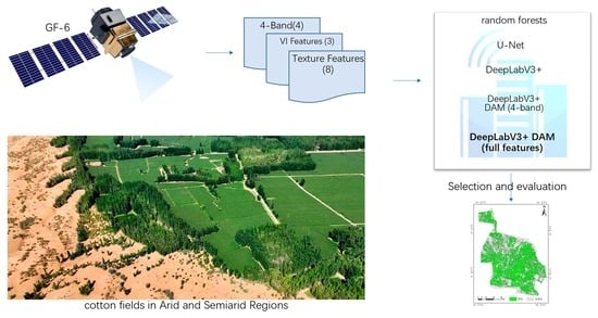
:Accurately grasping the distribution and area of cotton for agricultural irrigation scheduling, intensive and efficient management of water resources, and yield estimation in arid and semiarid regions is of great significance. In this paper, taking the Xinjiang Shihezi oasis agriculture region as the study area, extracting the spectroscopic characterization (R, G, B, panchromatic), texture feature (entropy, mean, variance, contrast, homogeneity, angular second moment, correlation, and dissimilarity) and characteristics of vegetation index (normalized difference vegetation index/NDVI, ratio vegetation index/DVI, difference vegetation index/RVI) in the cotton flowering period before and after based on GF-6 image data, four models such as the random forests (RF) and deep learning approach (U-Net, DeepLabV3+ network, Deeplabv3+ model based on attention mechanism) were used to identify cotton and to compare their accuracies. The results show that the deep learning model is better than that of the random forest model. In all the deep learning models with three kinds of feature sets, the recognition accuracy and credibility of the DeepLabV3+ model based on the attention mechanism are the highest, the overall recognition accuracy of cotton is 98.23%, and the kappa coefficient is 96.11. Using the same Deeplabv3+ model based on an attention mechanism with different input feature sets (all features and only spectroscopic characterization), the identification accuracy of the former is much higher than that of the latter. GF-6 satellite image data in the field of crop type recognition has great application potential and prospects.
1. Introduction
Cotton is the most produced and utilized natural fiber worldwide. It is not only an important raw material for the development of the textile industry but also an oil crop and fine chemical raw material. As the largest producer and consumer of cotton in the world, China plays an important role in global cotton production, consumption, and trade. Cotton is one of the most important cash crops in China, and it is directly related to the national economy and people’s livelihood. Additionally, cotton cultivation is closely related to irrigation and also has a serious impact on total nitrogen emissions during the growing season. Xinjiang is the largest cotton producer in China, but it is located in an arid and semiarid region with severe water scarcity. Moreover, global warming intensifies and accelerates potential evaporation from crop surfaces, so a decline in the availability of soil moisture to plants is obvious, and indirectly, the agricultural water demand has increased [1]. With the development of society, the increase in water consumption in industries and domestically has led to a decrease in the available water for agriculture, exacerbates the supply–demand contradiction of agricultural water use, and seriously affects the sustainable development of agriculture [2]. In addition, the flowering and boll stage is the most highly sensitive period of cotton to water and fertilizer demand, and it is also a period of centralized irrigation for cotton. Optimizing the irrigation scheduling strategy, managing water resources intensively and efficiently, and improving cotton water productivity are urgent challenges to be solved in arid and semiarid agriculture regions [3]. Therefore, accurately measuring and analyzing the spatial distribution characteristics of early cotton is a basic prerequisite of agricultural water management and optimization in Xinjiang in order to provide strong support for the adjustment of regional economic structure, industrial structure, and water resource scheduling.
Traditional information about crop planting area, yield, and other data is mainly obtained by on-the-spot sampling survey methods, and then those reports are gathered and submitted step-by-step, which is not suitable for large-scale surveillance of agriculture information. However, such investigations involve a tremendous amount of work, lack quality control, and cannot provide spatial distribution information, making it difficult to meet the needs of modern management and decision-making. Satellite remote sensing, as an advanced detection technique for the recognition of ground objects, can obtain real-time information on a large scale from ground objects and has played an important role in cotton recognition [4,5]. With the steady development of sensor performance, cotton recognition has evolved from lower spatial resolution and multispectral remote sensing image data [6,7,8] to high spatial resolution and hyperspectral remote sensing imagery [9,10], and its recognition degree and accuracy are constantly improving. Moreover, although the recognition and accuracy of images obtained by drones equipped with cameras are very high [11], and the sampling time can be flexibly controlled, the observation range is smaller than satellite remote sensing, the cost of field operations is high, and large-scale surveillance of agriculture information requires a long cycle, making it unsuitable for early crop recognition. In recent years, experts and scholars have conducted extensive research on the extraction of cotton planting areas based on multitemporal or multi-source remote sensing image data [12,13]. Although it can achieve good recognition results, the recognition process is complex, and early identification of cotton remote sensing cannot be completed in time. Moreover, the interference of cloud cover and rather long revisiting cycles of high-resolution satellite exists, making it difficult to obtain multitemporal remote-sensing data during the cotton growth period, which brings many difficulties to the research of cotton recognition [14]. At present, various classification methods based on pixels or objects have been used for remote-sensing recognition of crops [15], such as the maximum likelihood method [16], nearest neighbor sampling method [17], spectral angle mapping method [18], decision tree algorithm [19], ear cap transformation method [20], support vector machine [21], random forest [22], neural network [23], and biomimetic algorithm [24]. For example, Ji Xusheng et al. [25] compared the recognition accuracy of different algorithms based on single high-resolution remote sensing images from specific time periods: SPOT-6 (May), Pleiades-1 (September), and WorldView-3 (October). With the rapid development of remote-sensing information deep excavation and information extraction technology, a series of crop classification algorithms and studies that do not rely on field sampling have also been carried out [26,27,28]. MARIANA et al. [29] used pixel-based and object-based time-weighted dynamic time to identify crop planting areas based on sentinel2 images, and this type of algorithm is becoming increasingly mature. Deep learning methods have been extensively used to extract valuable information due to their ability to extract multiple features of remote sensing images and to discover more subtle differences, as well as their high training efficiency and classification accuracy and the ability to reduce significant spectral differences within similar ground objects (such as “same object but different spectra” and “foreign object with the same spectrum” phenomena) [30]. Research has shown that convolutional neural networks (CNN) have powerful feature learning and expression capabilities [31]. Zhang Jing et al. [32] used drones to obtain RGB images of six densities of cotton fields and expanded the dataset using data augmentation technology. Different neural network models (VGGNet16, GoogleNet, MobileNetV2) were used to identify and classify cotton fields with different densities, with recognition accuracy rates exceeding 90%. However, under the higher-yield-technique mode of mechanized farming in Xinjiang, the plant spacing between plants and rows is unified. The classification of density does not have practical significance unless there is a lack of seedlings due to disasters. The existing high-resolution temporal and spatial research projects of cotton recognition and area extraction mostly focus on the comprehensive utilization of medium-resolution multitemporal images [33,34]. There is little research on remote-sensing image recognition of a single period or critical period in cotton growth, especially in early cotton based on high-resolution remote-sensing images. Moreover, in large-scale cotton operations, the advantages of object-oriented analysis and design methods of early recognition in high-resolution images are not clear, and further research and exploration are needed.
DeepLabV3+ network is a CNN that can be used for pixel-level object detection. Due to the performance in locating objects in images with complex backgrounds, this type of method has been widely applied in the field of agriculture [35,36]. In this study, an improved DeepLab V3+ network method for cotton high-resolution remote sensing recognition has been proposed, termed DAM (double attention mechanism), to recognize cotton. By adding a DAM module, it is possible to highlight the important parts of channels and spaces in the recognition results, thereby improving the precision of the recognition results. Furthermore, the red edge band can effectively monitor the growth status of vegetation. GF-6 satellite is the first multispectral remote sensing satellite in China to be equipped with a red edge band alone. The monitoring capabilities of satellites for resources such as agriculture, forestry, and grasslands can be improved. Improving the classification accuracy of paddy crops and enhancing crop recognition capabilities by red edge information, purple band, and yellow band showed the GF-6 satellite had broad application prospects in the precise identification and area extraction of crops. Given the outstanding performance on recognition in the field of agriculture by using the DeepLab V3+ network and GF-6 images recently, we considered applying this improved DeepLabV3+ network structure on cotton field identification and compare the results with other models to see its performance at identifying the cotton field. The purpose of this study is to provide a fast and efficient method for the early large-scale identification and distribution of cotton, better serving the critical irrigation period of cotton in arid and semiarid regions and providing a good decision-making basis for water-saving irrigation policies in arid and semiarid regions.
2. Materials and Methods
2.1. Study Area
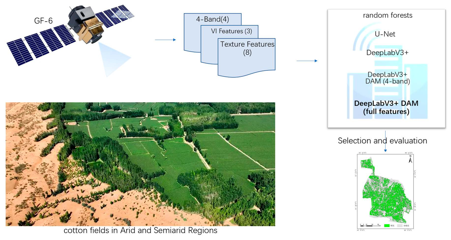
Shihezi Reclamation Area in Xinjiang (E84°58′–86°24′, N43°26′–45°20′) is located in the middle of the northern foot of the Tianshan Mountains, in the south of the Junggar Basin and connected to Gurbantunggut Desert in the north, with a total area of 5.851 × 10⁹ m3 (Figure 1). The terrain, from south to north, is divided into the Tianshan Mountains, piedmont hilly areas, piedmont inclined plains, flood alluvial plains, and aeolian desert areas, with an average elevation of 450.8 m. The soil is mostly composed of gray desert soil, fluvo-aquic soil, and meadow soil. The soil is mainly composed of gravel soil, sandy soil, clay soil, etc. Winter is long and cold, and summer is short and hot, with an annual average temperature of 7.5–8.2 °C, 2318–2732 h of sunshine, 147–191 days of frost-free period, 180–270 mm of annual rainfall, and 1000–1500 mm of annual evaporation. Atmospheric water resources (water vapor resources and cloud water resources) are relatively less compared to other regions in China, and the climate is arid, belonging to a typical temperate continental climate. There are rivers and springs on the surface, as well as three rivers, including the Manas River, Jingou River, and Bayingou River, within the territory. The water source of drip irrigation for cotton fields is “groundwater plus canal water”.
2.2. Data Sources
GF-6 is a low-orbit optical remote-sensing satellite. As China’s first precision agriculture high-resolution observation satellite, the high-resolution camera (PMS) uses a TDICCD detector that combines panchromatic and blue (450–520 nm), green (520–600 nm), red (630–690 nm), and near-infrared (760–900 nm) spectra with a panchromatic resolution of 2 m and a multispectral resolution of 8 m. Both panchromatic and multispectral systems share the same optical system, and interference filters are used for spectral analysis. Both push-sweep widths are 95 km, with a spectral range of 450–900 nm. The data is downloaded from the China Resources Satellite Application Center Network (https://www.cresda.com/zgzywxyyzx/index.html (accessed on 20 June 2022, 28 June 2022)). Collect GF-6 satellite PMS image data on 20 June 2022 (Jing No. 549536), 20 June (Jing No. 549537), and 28 June (Jing No. 552234), covering the entire study area during the cotton flowering period.
2.3. Data Processing
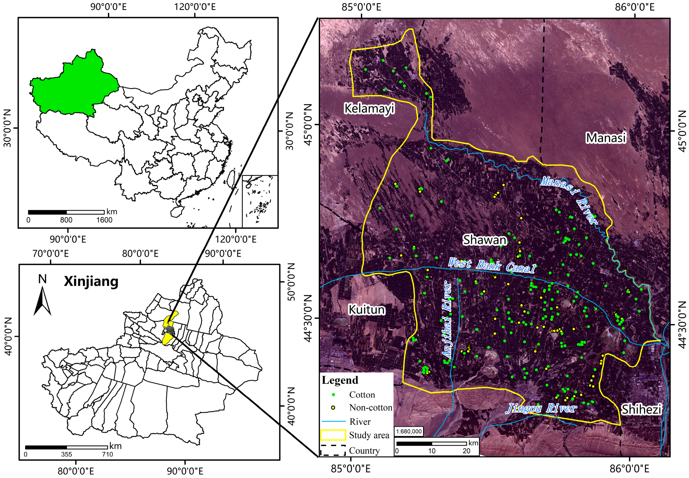
Image preprocessing includes five parts: radiometric calibration, atmospheric correction, orthophoto correction, data fusion, and sample labeling. Firstly, radiation calibration, atmospheric correction, and orthophoto correction are performed on multispectral data, while atmospheric correction is not performed on panchromatic data. Secondly, by fusing the preprocessing panchromatic and multispectral images, the image resolution can reach up to 2 m. Next, band synthesis is performed, and texture features are extracted using the Gray Level Co-occurrence Matrix (GLCM). Then, select representative desert oasis transition zones, urban areas, plantations, and various terrain mixed areas within the image for cotton labeling and generate a binary vector layer with ID 2 (cotton) and ID 1 (non-cotton). Finally, convert the vector layer into a grid layer and crop it (Figure 2). This study utilizes image rotation and image flipping to enhance data and increase samples in the training set.
2.4. Model and Parameter
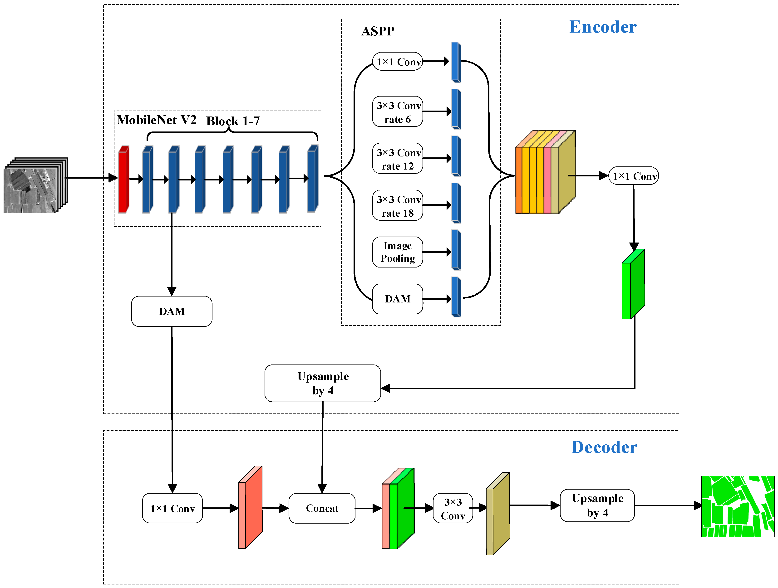
DeepLabV3+ combines the advantages of the EnCoder-Decoder (ED) structure and the Atrus Spatial Pyramid Pooling (ASPP) module. To make the model more suitable for identification of cotton, this paper has made the following improvements on the basis of DeepLabV3+, changing the backbone network (Xception network) to a more lightweight MobileNet V2 network. Secondly, in order to increase the sensitivity of the model to the cotton planting area, AM (attention mechanism) was added to the ASPP module and upsampling layer. The network architecture diagram of the DeepLabV3+ semantic segmentation model based on the attention mechanism is shown in Figure 3.
MobileNet V2 can learn more complex features with fewer parameters and lower computational costs compared to traditional convolutional networks. Simultaneously, having an inverted residual structure helps to increase the network’s representation ability while maintaining its efficiency [37].
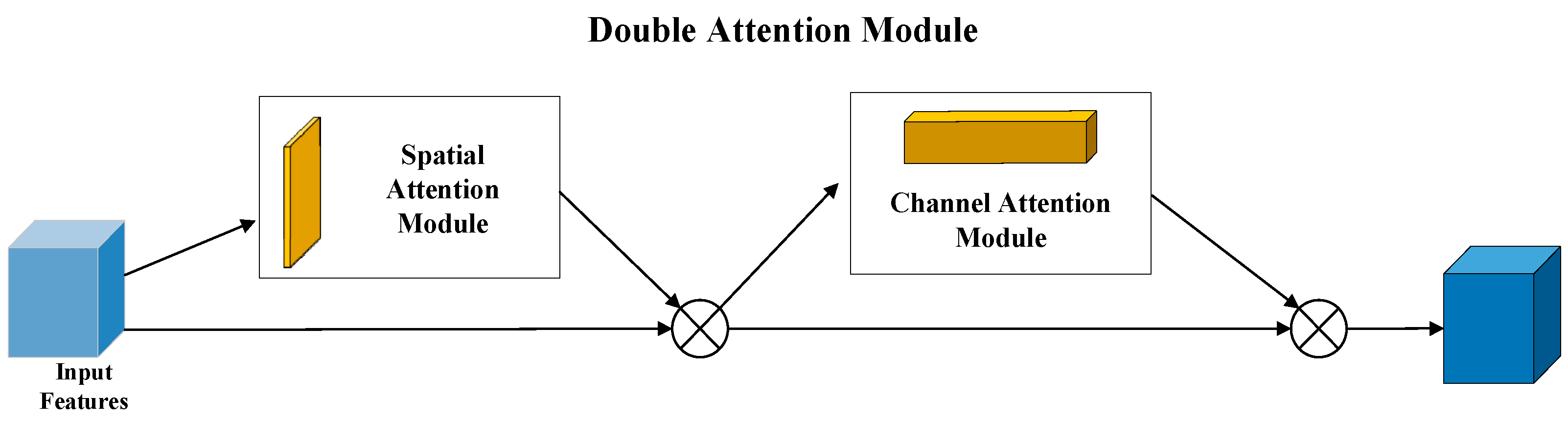
Visual attention is an inherent mechanism that plays an important role in human visual perception. As our visual system has limited capacity and cannot efficiently process the information from the entire visual field, we focus our attention on specific areas of interest in the image and utilize local observation to focus on the prominent parts for detailed analysis of these areas. In recent years, many experts and scholars have added attention mechanisms to network models to improve recognition performance [38,39]. The DAM is a combination of a spatial attention module and a channel attention module. By adding a DAM module, it is possible to highlight the important parts of channels and spaces in the recognition results, thereby improving the precision of the recognition results [35]. The DAM structure diagram is shown in Figure 4.
The spatial attention module can highlight the spatial position distribution that is important for recognition in the convolutional layer. By performing channel compression on the input feature map F through global average pooling and global maximum pooling, and are obtained respectively. After merging two feature maps, the dimensionality is reduced to 1 channel through a 7 × 7 convolution operation. Then, the weight map of spatial attention is generated through the Sigmoid function, and the generated weight map is multiplied by the original feature map (F) to obtain the spatial attention weighted map (). Its formula is as follows:
In the equation, σ represents the sigmoid function, f7 × 7 represents the convolution of 7 × 7, ⊕ represents channel merging, and ⊗ represents element multiplication.
The channel attention module can highlight channels of significant value for recognition in the convolutional layer. By compressing the spatial dimensions of the feature map (F) through global average pooling and global maximum pooling, and are obtained. Then, input Fmaxc and Favgc into a multi-layer perceptron (MLP), add the obtained results, and input the sigmoid function to generate the weight of the channel attention. Multiply the generated weight with the original feature map (F) to obtain the channel attention-weighted map (). Its formula is as follows:
In the equation, σ represents the sigmoid function, MLP represents the multi-layer perceptron, ⊕ represents channel merging, and ⊗ represents element multiplication.
2.5. Feature Set Construction
2.5.1. Vegetation Index Features
The vegetation index has regional and temporal characteristics, which are influenced by various factors such as atmospheric conditions, surrounding environment, lighting conditions, and vegetation growth. It also varies depending on the season or surrounding environment. Due to the values of the Normalized Vegetation Index (NDVI) being between [−1,1], it can avoid inconvenience in subsequent data calculations and partially mitigate the effects caused by factors such as terrain, cloud shadows, solar altitude angle, and satellite observation angle. The ratio vegetation index (RVI) has a high correlation with the leaf area index and chlorophyll content and can be used to distinguish different crops. The difference vegetation index (DVI), also known as the environmental vegetation index, is extremely sensitive to changes in the environment. Therefore, attempts were made to identify cotton using NDVI, RVI, and DVI (Table 1).
2.5.2. Texture Features
Texture feature is an inherent feature of an image, which reflects the properties and spatial relationships of the grayscale of the image. It accurately reflects the real structure of ground objects through the frequency of color tone changes in the image. The presence of differences in canopy structure among different crops is an important classification feature for crop recognition [40].
Based on the fused 4-band data of GF-6 PMS, the principle of Gray Level Co-occurrence Matrix (GLCM) proposed by Haralick is introduced to extract texture features. The eight texture feature parameters include entropy (ENT), mean (MEA), variance (VAR), contrast (CON), homogeneity (HOM), second moment (ASM), correlation (COR), and dissimilarity (DIS) [41]. In calculation, the parameters involved are the window size, direction, step length, etc.
2.5.3. Feature Combination
In order to compare the recognition accuracy of different models and the recognition accuracy using only the 4-band features and full features under the DeepLabV3+ network attention mechanism model, the following experiments were conducted, and their recognition accuracy was compared (Table 2).
2.6. Model Performance Evaluation Indicators
The semantic segmentation performance evaluation indicators can be used to compare the recognition results. There are many indicators commonly used to evaluate the performance of model training processes, such as Pixel Accuracy (PA), Mean Intersection over Union (MIoU), Precision, Recall, F1_Score, Intersection over Union, IoU, etc. This paper uses MIoU and cross-entropy loss function as evaluation indicators.
IoU is used to evaluate the overlap between each class and the real label in the semantically segmented image. The confusion matrix (CM) of identification results is shown in Table 3. The calculation formula is
TP and TN with predicted values consistent with actual values; FP, FN with inconsistent predicted and true values.
MIoU calculates the mean of all classes of IoU using the following formula:
Binary cross entropy is a loss function commonly used in machine learning modules to evaluate the quality of a binary classification prediction result. Its formula is
where y is the binary label 0 or 1, and is the probability that the output belongs to the y label. For the case where label y is 1, if the predicted value approaches 1, then the value of the loss function approaches 0. On the contrary, its value is very large, which is very consistent with the properties of the log function.
2.7. Model Parameter Settings
The parameters of the DeepLabV3+ network attention mechanism model used in this paper are shown in Table 4:
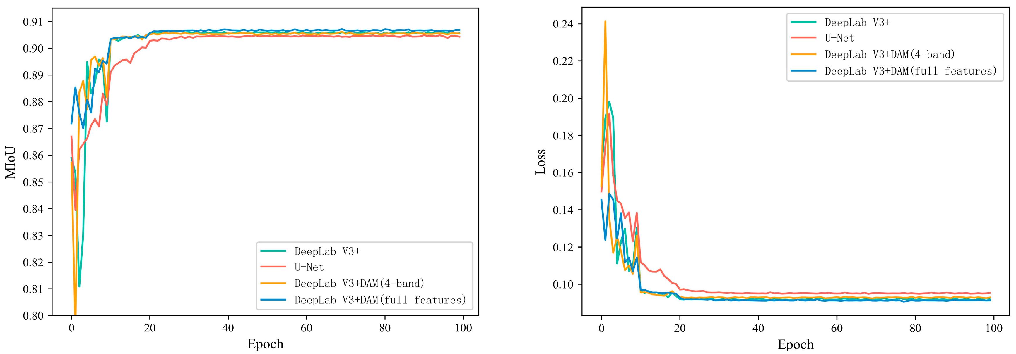
Batch size represents the data volume input into GPU graphics memory each time. Epoch represents the number of iterations after a complete traversal during deep learning model training. Through continuous attempts, the model achieves satisfactory results when Epoch is 100 in this paper. The Adam optimizer function is used as the parameter optimizer. Using a dynamically decaying learning rate and the StepLR function provided in the PyTorch model, the initial learning rate is set to 0.01, step size is set to 10, and gamma is set to 0.1. This indicates that the learning rate decreases to 0.1 times the original after every 10 iterations (Figure 5). In this paper, horizontal and vertical flipping were used to increase the sample size. After the data preprocessing is completed, the vectorized sample data is made into label data in the study area, and it is randomly divided into training samples and validation samples in a 7:3 ratio. This study used this label data to evaluate the performance of deep learning models (U-Net, DeepLabV3+, DeepLabV3+ DAM with 4-band, and DeepLabV3+DAM with full features).
2.8. Model Accuracy Evaluation Indicators
This paper verifies the accuracy through on-site observation data and selects 98 non-cotton sample points and 185 cotton sample points in the study area. Calculate the CM using omission error and commission error, then derive the consistency of the kappa coefficient and overall accuracy between the classification map and the reference data. Calculate classification accuracy statistical data based on the error matrix, including overall accuracy (correct classification number/total number of measured samples), producer’s accuracy (correct classification number/total number of a certain category), user’s accuracy (correct classification number/(correct classification number plus total number of misclassified to a certain category)), and kappa coefficient. This study used this on-site observation data to evaluate the accuracy of all models.
The Kappa coefficient is an indicator for comprehensive evaluation of classification accuracy, which can determine the consistency of classification [42]. Its formula is
where Po is the sum of the correct pixel count for cotton and non-cotton classification divided by the total number of pixels. Assuming that the true pixel count for each class is {x1, x2}, the predicted pixel count for each class is {y1, y2}, and the total number of pixels in the sample is n, Pe is calculated as follows:
3. Results and Analysis
3.1. Performance Evaluation
In view of the excellent performance of the DeepLabV3+ network model in image recognition, we consider applying this improved DeepLabV3+ network attention mechanism model structure to cotton field recognition and comparing its performance with other models to see its performance in early cotton recognition to see its performance in the early identification of cotton. Considering the training efficiency and cotton recognition accuracy, this paper also compares the attention mechanism model of the DeepLabV3+ network using only 4-band.
MIoU can be used to judge the accuracy of the model’s prediction results and labeled as similar, and the speed of the model’s operation can also be determined based on the calculation speed. It is a relatively balanced indicator for measuring model performance. By comparing the training sets in the dataset (Table 5), it is found that the DeepLabV3+ network attention mechanism model with full features has the highest MIoU and the minimum binary cross entropy loss function. Through comparing the MIoU and the binary cross entropy loss function, we can find that although the DeepLabV3+DAM with full features performs the best regarding MIoU and loss, these optimal values show a very small absolute difference between these key performance indicators.
3.2. Accuracy Evaluation
CM is the most important index in the accuracy evaluation of ground object recognition. The omission error and commission error can be expressed by producer precision and user precision, respectively. Therefore, overall accuracy, producer accuracy, user accuracy, and Kappa coefficient are used to compare the accuracy of different model algorithms’ recognition results (Table 5). It was found that in the model using full feature information for classification, the overall accuracy of the DeepLabV3+ network was 96.11%, while the overall accuracy of the model incorporating the attention mechanism was 98.23%, an improvement of 2%. The Kappa coefficient also increased from 0.914 to 0.961, an increase of 0.047. However, the overall classification accuracy and Kappa coefficients of the 4-band DeepLabV3+ network with attention mechanism are less different from those of the DeepLabV3+ network with all feature sets, and the recognition accuracy of the five comparisons reaches an excellent level except RF (0.8 ≤ Kappa ≤1) [43].
From Table 6, the DeepLabV3+ DAM with all feature sets shows that the producer’s accuracy of cotton is 98.38%, while the user’s accuracy of cotton is 98.91%. This indicates that 98.38% of the cotton area on the ground is correctly identified as cotton, while 98.91% of the estimated cotton area on the classification map is actually cotton. In other words, the classification map missed 1.62% of the cotton area on the ground (omission error), while approximately 1.09% of the pixels classified as cotton on the classification map (commission error) actually belong to other categories. Among the 185 measured points that were actually cotton, 3 points were misclassified as non-cotton. In addition, out of the 184 points classified as cotton on the classification map, 2 are actually corn. Indirectly, the actual cotton area is underestimated on the classification chart, but not much, only 0.53%. Among the evaluation indicators of P_A, U_A, Overall accuracy, Kappa, MIoU, and Loss, the performance and accuracy indicators of the DeepLabV3+DAM with full features perform best. Therefore, the DeepLabV3+DAM with full features can be concluded to have the best performance and accuracy for the cotton early identification task in our study when considering the general probability.
3.3. Cotton Identification
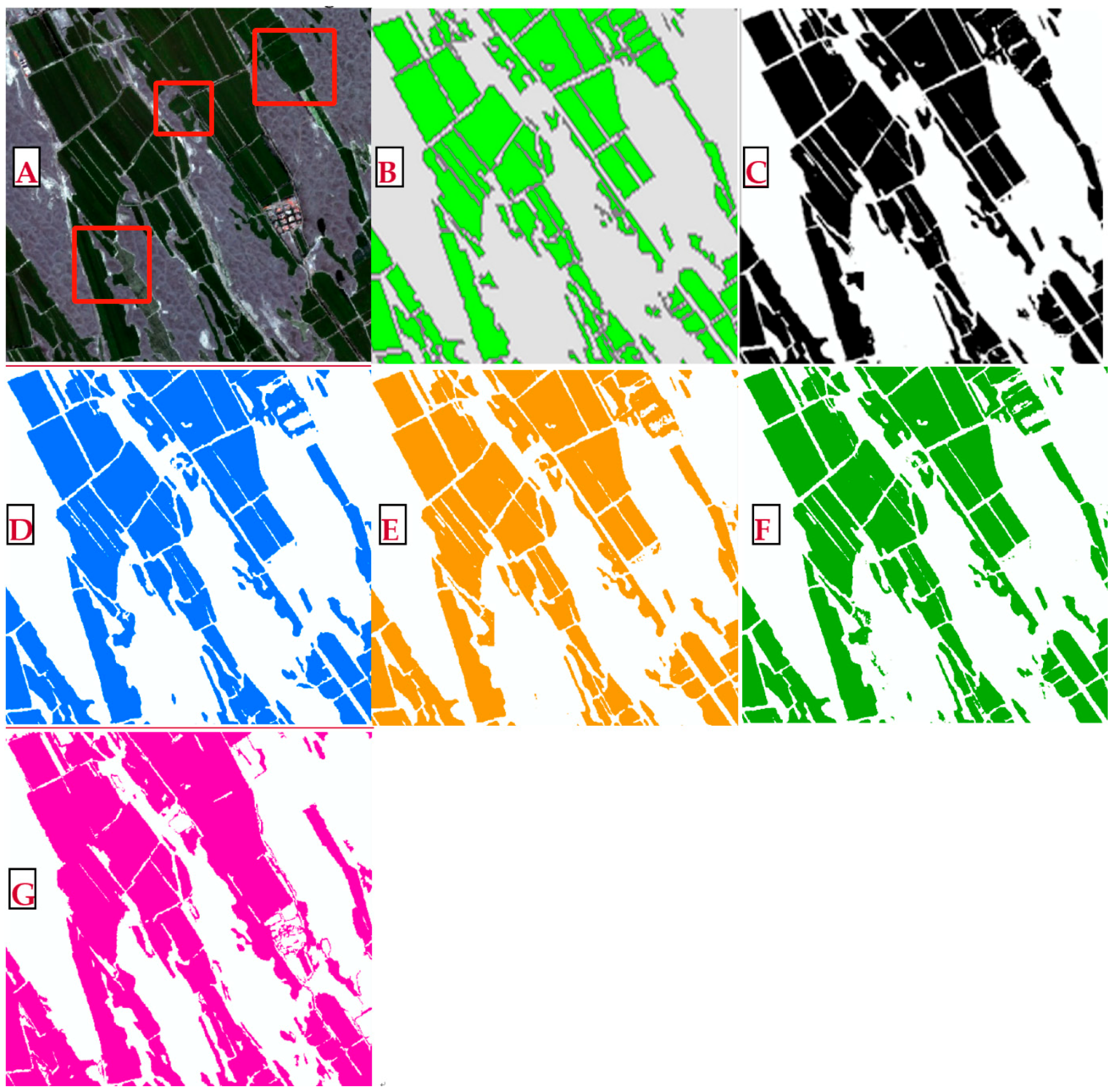
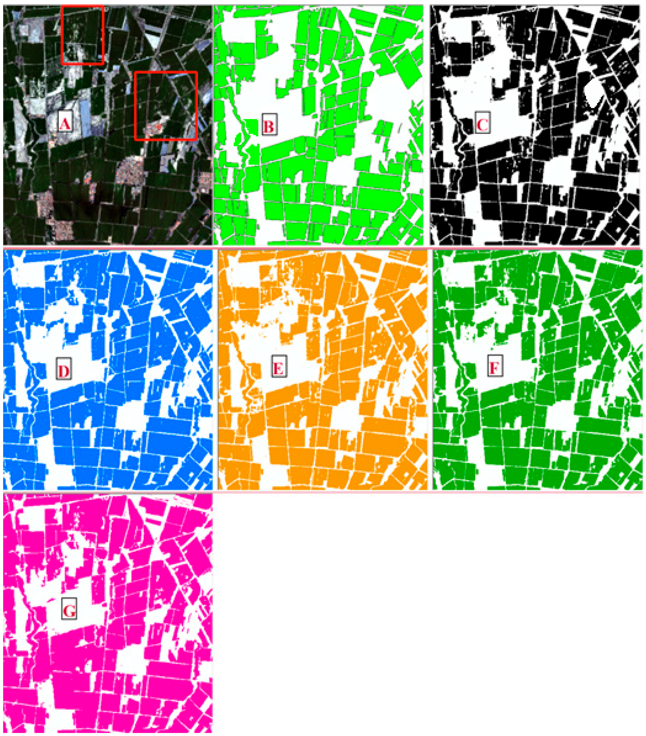
Based on GF-6 satellite images, cotton is identified by comprehensive use of spectrum, its combination information, and texture information. We compare its performance and accuracy for the cotton early identification task with the RF, U-Net, DeepLabV3+ network, and Deeplabv3+ model based on the attention mechanism with 4-band. According to the above description, applying the DeepLabV3+DAM model proposed in this article to remote sensing recognition of cotton can achieve higher recognition accuracy and extraction effect. Therefore, we visualize the detailed features of five sub-images, the corresponding ground truths, and the prediction results of different models from the validation dataset. These five areas include representative desert oasis transition zones, urban areas, plantation areas, and various terrain mixed areas. Considering the training efficiency and cotton identification accuracy, we selected a portion of the representative desert oasis transition zones in the GF-6 images to exhibit each model’s performance. The recognition results are shown in Figure 6. We can see that the DeepLabV3+DAM with full features predictions (Figure 6C) are the most consistent with the original image (Figure 6A) and visual interpretation samples (Figure 6B), while the RF predictions (Figure 6G) are relatively rough. From the visual interpretation, the accuracy of DeepLabV3+DAM with full features is better than the other models on the discrimination between cotton and non-cotton fields, without excessive confusion and misjudgment in desert oasis transition zones, and other models have excessive confusion and misjudgment in the red solid line depicts area. In addition, except for the RF model, the boundaries of the cotton fields in other models are relatively clear in desert oasis transition zones, indicating that deep learning is superior to machine learning in this recognition experiment. This is because by modifying the input layer and adding an upsampling layer, the phenomenon of loss of ground object boundary information is improved, and the recognition accuracy of cotton is improved.
Considering the training efficiency and cotton identification accuracy, we selected another portion of the representative urban area in the GF-6 images to exhibit each model’s performance. By comparing their performance and accuracy for the cotton early identification model of the RF, U-Net, DeepLabV3+ network, and Deeplabv3+ DAM with 4-band, the recognition results are shown in Figure 7. We can see that the prediction results of all the deep learning methods (Figure 7C) are similar to the original image (Figure 7A) and visual interpretation samples (Figure 7B), while the RF predictions (Figure 7G) are relatively rough. From the visual interpretation, the accuracy of DeepLabV3+DAM with full features is better than the other models on the discrimination between cotton and non-cotton fields. There are only a few instances of excessive confusion and misjudgment in the representative urban area, and other models have more excessive confusion and misjudgment than DeepLabV3+DAM with full features model in the red solid line depicts area. In addition, except for the RF model, the boundaries of the cotton fields in other models are also relatively clear in the representative urban area, indicating that deep learning is superior to machine learning in this recognition experiment. It has been determined to be the best model for early cotton recognition in view of the excellent performance of the DeepLabV3+DAM model with full features in previous experiments. In this research, under the premise of limited training samples, the DeepLab V3+ ADM model still achieved good results for early cotton recognition and can provide a decision-making basis for water-saving irrigation in this area.
4. Conclusions and Discussion
4.1. Conclusions
In this paper, the improved DeepLabV3+DAM model structure—which was used for the field of agriculture previously [35,36] to identify cotton fields using GF-6 satellite image data—is shown. This model can introduce the DAM module, which is a combination of the spatial attention module and channel attention module. The spatial attention module can highlight the spatial position distribution that is important for recognition in the convolutional layer. The channel attention module can highlight channels of significant value for recognition in the convolutional layer. By modifying the input layer and adding an upsampling layer, the phenomenon of loss of ground object boundary information is improved, and the recognition accuracy of cotton is improved. Based on this advantage, the model can fully use spectral combination information and texture information for cotton field identification before and after the flowering period of cotton. These experiment results have been validated using ground truths and compared with four deep learning models (U-Net, DeepLabV3+, DeepLabV3+ DAM with 4-band, DeepLabV3+ DAM with full features) and a machine learning model (RF). Through experiments, it can be found that the recognition results are affected by many factors, such as reflection spectrum, ground texture information, and model algorithm. The main conclusions are as follows:
According to the experimental results, the improved DenseNet model is superior to these popular CNNs using the same datasets.
- (1)
- The recognition accuracy of traditional machine learning algorithms is far inferior to that of deep learning algorithms in accuracy evaluation and the phenomenon of loss of ground object boundary information.
- (2)
- Compared with the DeepLab V3+ network and U-Net, the DeepLabV3+ DAM model with the full feature showed a good effect on early cotton recognition in this study area.
- (3)
- Only the spectral information provided by the 4-band feature set is relatively limited, and the performance and recognition accuracy of the same DeepLabV3+ DAM model is worse than that of the full feature set.
4.2. Discussion
In this research, from the perspective of water conservation and regulation, high-resolution images of the cotton flowering period were obtained. The conclusion that previous studies from the perspective of yield estimation have found that the highest cotton recognition accuracy in this region occurs during the boll opening period (August, September) [8,44] is not contradictory. The low coverage rate of cotton in the flowering stage and the unified mechanical cultivation mode of cotton in Xinjiang provided the basis for the selection of the texture feature sets and laid the foundation for improving the accuracy of early cotton remote-sensing recognition and reduce the difficulty of recognition. However, it should be noted that if there are other crops using wide film drip irrigation in the study area during the same period, it is likely to cause confusion in the recognition results, such as the only two misclassifications in the DeepLab V3+ DAM model being corn. A future task will be to verify the improved DeepLab V3+ DAM model on images with higher temporal, spatial, and spectral resolutions for cotton field identification. Early recognition based on drone cotton has been used by many scholars for pest control due to its high spatial resolution and free time control [45,46]. However, it is time-consuming and expensive, and flight time and area are strictly controlled. In addition, the later image stitching method will also affect recognition accuracy, which is slightly less economical and practical compared to high-resolution remote sensing image recognition. The second future task is to apply this method in other areas with complex planting structures and diversified agricultural management practices. Xun et al. [5] explored the feasibility of combining time series enhanced vegetation index (EVI) calculated from Moderate Resolution Imaging Spectroradiometer (MODIS) satellite data with the fused representation-based classification (FRC) algorithm to identify the cotton pixels and map cotton cultivated area in the major cotton production regions of China. They believe that the accuracy of the model is influenced not only by longitude and latitude but also by agricultural management practices (such as species and sowing dates) and climate change. Compared with using only 4-band satellite images based on remote-sensing image (GF-1, WFV) data to identify cotton during the boll opening period [47], it is believed that the optimized model of DenseNet can fully utilize spatial and spectral information for cotton field recognition. By comparing the training efficiency and performance of four widely used classical convolutional neural networks (ResNet, VGG, SegNet, and DeepLab v3+), it was also found that the DeepLab V3+ network has the shortest training time, the easiest training, and the lowest computational cost. So, the third future task is to reduce the labor cost, improve the automation level and working efficiency of the model, and improve the stability and generalization of the model.
Author Contributions
Data curation, H.L.; writing—original draft preparation, C.Z.; writing—review and editing, D.C.; investigation, J.Z.; visualization, J.F. and Z.C.; supervision, Z.W.; project administration, H.Z. All authors have read and agreed to the published version of the manuscript.
Funding
This research was funded by the Major science and technology Project of High-Resolution Earth Observation System, grant number 76-Y50G14-0038-22/23; Anhui Science and Technology Major Program grant number 202003a06020002; Key Research and Development Program of Anhui Province grant number 2021003; the Science Foundation for Distinguished Young Scholars of Anhui Universities grant number 2022AH020069; Collaborative Innovation Project of Universities in Anhui Province grant number GXXT-2021-048; Anhui Provincial Special Support Plan grant number 2019; Science Research Key Project of Anhui Educational Committee grant number 2023AH051603; Key Natural Science Research Project of Anhui Provincial Colleges Grant number 2023AH050137; Key Project of Anhui Provincial College Excellent Youth Talents Support Program in 2022 Grant number 13.
Conflicts of Interest
The authors declare no conflict of interest.
References
- Zhao, C.; Shanm, L.; Deng, X.; Zhao, L.; Zhang, Y.; Wang, S. Current situation and counter measures of the development of dryland farming in China. Trans. CSAE 2004, 40, 280–285. [Google Scholar]
- Wu, P.; Zhao, X. Impact of climate change on agricultural water use and grain production in China. Trans. CSAE 2010, 26, 1–6. [Google Scholar]
- Shi, J.; Du, Y.; Du, J.; Jiang, L.; Chai, L.; Mao, K. Progress in Microwave Remote Sensing Surface Parameter Inversion. Sci. China Earth Sci. 2012, 42, 814–842. [Google Scholar]
- Xun, L.; Zhang, J.; Yao, F.; Cao, D. Improved identification of cotton cultivated areas by applying instance-based transfer learning on the time series of MODIS NDVI. Catena 2022, 213, 106130. [Google Scholar] [CrossRef]
- Xun, L.; Zhang, J.; Cao, D.; Wang, J.; Zhang, S.; Yao, F. Mapping cotton cultivated area combining remote sensing with a fused representation-based classification algorithm. Comput. Electron. Agric. 2021, 181, 105940. [Google Scholar] [CrossRef]
- Genbatu, G.; Shi, Z.; Zhu, Y.; Yang, X.; Hao, Y. Land use/cover classification in an arid desert-oasis mosaic landscape of china using remote sensed imagery: Performance assessment of four machine learning algorithms. Glob. Ecol. Conserv. 2020, 22, e00971. [Google Scholar]
- Yang, B.; Pei, Z.; Jiao, X.; Zhang, S. Cotton growing area monitoring in Northwest China using CBERS-1 data based on satellite remote sensing. Trans. CSAE 2003, 19, 4. [Google Scholar]
- Cao, W.; Yang, B.; Song, J. Spectral information based model for cotton identification on Landsat TM Image. Trans. CSAE 2004, 20, 112–116. [Google Scholar]
- Wang, C.; Chen, Q.; Fan, H.; Yao, C.; Sun, X.; Chan, J.; Deng, J. Evaluating satellite hyperspectral (Orbita) and multispectral (Landsat 8 and Sentinel-2) imagery for identifying cotton acreage. Int. J. Remote Sens. 2021, 41, 4042–4063. [Google Scholar] [CrossRef]
- Raza, D.; Shu, H.; Khan, S.; Ehsan, M.; Saeed, U.; Aslam, H.; Aslam, R.; Arshad, M. Comparative geospatial approach for agricultural crops identification in inter- fluvial plain- A case study of Sahiwal district, Pakistan. Pak. J. Agric. Sci. 2022, 59, 567–578. [Google Scholar]
- Ma, Y.; Ma, L.; Zhang, Q.; Huang, C.; Yi, X.; Chen, X.; Hou, T.; Lv, X.; Zhang, Z. Cotton Yield Estimation Based on Vegetation Indices and Texture Features Derived from RGB Image. Front. Plant Sci. 2022, 13, 925986. [Google Scholar] [CrossRef] [PubMed]
- Ahsen, R.; Khan, Z.; Farid, H.; Shakoor, A.; Ali, A. Estimation of cropped area and irrigation water requirement using Remote Sensing and GIS. J. Appl. Pharm. Sci. 2020, 30, 876–884. [Google Scholar]
- Conrad, C.; Fritsch, S.; Zeidler, J.; Cker, G.; Dech, S. Per-field irrigated crop classification in arid Central Asia using SPOT and ASTER data. Remote Sens. 2010, 2, 1035–1056. [Google Scholar] [CrossRef]
- Sanchez, A.; Gonzalez-Piqueras, J.; de la Ossa, L.; Calera, A. Convolutional Neural Networks for Agricultural Land Use Classification from Sentinel-2 Image Time Series. Remote Sens. 2022, 14, 5373. [Google Scholar] [CrossRef]
- Arvind; Hooda, R.; Sheoran, H.; Kumar, D.; Satyawan; Abhilash; Bhardwaj, S. RS-based regional crop identification and mapping: A case study of Barwala sub-branch of Western Yamuna Canal in Haryana (India). Indian J. Tradit. Knowl. 2020, 19, 182–186. [Google Scholar]
- Abouel, M.L.; Tanton, T. Improvements in land use mapping for irrigated agriculture from satellite sensor data using a multi-stage maximum likelihood classification. Remote Sens. 2003, 24, 4197–4206. [Google Scholar] [CrossRef]
- Samaniego, L.; Schulz, K. Supervised classification of agricultural land cover using a modified K-NN technique (mnn) and Landsat remote sensing imagery. Remote Sens. 2009, 1, 875–895. [Google Scholar] [CrossRef]
- Alganci, U.; Sertel, E.; Ozdogan, M.; Ormeci, C. Parcel-level identification of crop types using different classification algorithms and multi-resolution imagery in southeastern turkey. Photogramm. Eng. Remote Sens. 2013, 79, 1053–1065. [Google Scholar] [CrossRef]
- Wardlow, B.D.; Egbert, S.L.; Kastens, J.H. Analysis of time-series MODIS 250 m vegetation index data for crop classification in the us central great plains. Remote Sens. Environ. 2007, 108, 290–310. [Google Scholar] [CrossRef]
- Crist, E.P.; Cicone, R.C. Application of the tasseled cap concept to simulated thematic mapper data. Photogramm. Eng. Remote Sens. 1984, 50, 343–352. [Google Scholar]
- Ozdarici-Ok, A.; Ok, A.; Schindler, K. Mapping of Agricultural Crops from Single High-Resolution Multispectral Images—Data-Driven Smoothing vs. Parcel-Based Smoothing. Remote Sens. 2015, 7, 5611–5638. [Google Scholar] [CrossRef]
- Duro, D.C.; Franklin, S.E.; Dubé, M.G. A comparison of pixel-based and object-based image analysis with selected machine learning algorithms for the classification of agricultural landscapes using spot-5 hrg imagery. Remote Sens. Environ. 2012, 118, 259–272. [Google Scholar] [CrossRef]
- Liu, J.; Shao, G.; Zhu, H.; Liu, S. A neural network approach for enhancing information extraction from multispectral image data. Can. J. Remote Sens. 2005, 31, 432–438. [Google Scholar] [CrossRef]
- Omkar, S.N.; Senthilnath, J.; Mudigere, D.; Kumar, M.M. Crop classification using biologically-inspired techniques with high resolution satellite image. J. Indian Soc. Remote Sens. 2008, 36, 175–182. [Google Scholar] [CrossRef]
- Ji, X.; Li, X.; Wan, Z.; Yao, X.; Zhu, Y.; Cheng, T. Pixel-Based and Object-Oriented Classification of Jujube and Cotton Based on High Resolution Satellite Imagery over Alear, Xinjiang. Sci. Agric. Sin. 2019, 52, 997–1008. [Google Scholar]
- Kerwin, W.S.; Prince, J.L. The kriging update model and recursive space-time function estimation. IEEE Trans. Signal Process. 2002, 47, 2942–2952. [Google Scholar] [CrossRef]
- Petitjean, F.; Inglada, J.; Gancarski, P. Satellite image time series analysis under time warping. IEEE Trans. Geosci. Remote Sens. 2012, 50, 3081–3095. [Google Scholar] [CrossRef]
- Osman, J.; Inglada, J.; Dejoux, J.-F. Assessment of a markov logic model of crop rotations for early crop mapping. Comput. Electron. Agric. 2015, 113, 234–243. [Google Scholar] [CrossRef]
- Mariana, B.; Ovidiu, C. Sentinel-2 cropland mapping using pixel-based and object-based time-weighted dynamic time warping analysis. Remote Sens. Environ. 2018, 204, 509–523. [Google Scholar]
- Lv, Y.; Gao, Y.; Rigall, E.; Qi, L.; Dong, J. Cotton appearance grade classification based on machine learning. Procedia Comput. Sci. 2020, 174, 729–734. [Google Scholar] [CrossRef]
- Xu, X.; Du, M.; Guo, H.; Chang, J.; Zhao, X. Lightweight FaceNet based on MobileNet. Int. J. Intell. Sci. 2020, 11, 1–16. [Google Scholar] [CrossRef]
- Zhang, J.; Wang, Q.; Lei, Y.; Wang, Z.; Han, Y.; Li, X.; Xing, F.; Fan, Z.; Li, Y.; Feng, Z. Classification of cotton density by using machine learning and unmanned aerial vehicle images. China Cotton 2021, 48, 6–10, 29. [Google Scholar]
- Wang, X.; Qiu, P.; Li, Y.; Cha, M. Crops identification in Kaikong River Basin of Xinjiang based on time series Landsat remote sensing images. Trans. Chin. Soc. Agric. Eng. (Trans. CSAE) 2019, 35, 180–188. [Google Scholar]
- Liu, J.; Wang, L.; Yang, F.; Wang, X. Remote sensing estimation of crop planting area based on HJ time-series images. Trans. Chin. Soc. Agric. Eng. (Trans. CSAE) 2015, 31, 199–206. [Google Scholar]
- Wang, C.; Zhang, R.; Chang, L. A Study on the Dynamic Effects and Ecological Stress of Eco-Environment in the Headwaters of the Yangtze River Based on Improved DeepLab V3+ Network. Remote Sens. 2022, 14, 2225. [Google Scholar] [CrossRef]
- Peng, H.; Xue, C.; Shao, Y.; Chen, K.; Xiong, J.; Xie, Z.; Zhang, L. Semantic segmentation of litchi branches using DeepLabV3+model. IEEE Access 2020, 8, 164546–164555. [Google Scholar] [CrossRef]
- Sandler, M.; Howard, A.; Zhu, M.; Zhmoginov, A.; Chen, L.C. Mobilenetv2: Inverted residuals and linear bottlenecks. In Proceedings of the IEEE Conference on Computer Vision and Pattern Recognition, Salt Lake City, UT, USA, 18–22 June 2018; pp. 4510–4520. [Google Scholar]
- Seydi, S.T.; Amani, M.; Ghorbanian, A. A Dual Attention Convolutional Neural Network for Crop Classification Using Time-Series Sentinel-2 Imagery. Remote Sens. 2022, 14, 498. [Google Scholar] [CrossRef]
- Lin, Y.; Xu, D.; Wang, N.; Shi, Z.; Chen, Q. Road Extraction from Very-High-Resolution Remote Sensing Images via a Nested SE-Deeplab Model. Remote Sens. 2020, 12, 2985. [Google Scholar] [CrossRef]
- Hidayat, S.; Matsuoka, M.; Baja, S.; Rampisela, D.A. Object-Based Image Analysis for Sago Palm Classification: The Most Important Features from High-Resolution Satellite Imagery. Remote Sens. 2018, 10, 1319. [Google Scholar] [CrossRef]
- Haralick, R.M. Statistical and structural approaches to texture. Proc. IEEE 2005, 67, 786–804. [Google Scholar] [CrossRef]
- Aguilar, M.; Bianconi, F.; Aguilar, F.; Fernández, I. Object-based greenhouse classification from GeoEye-1 and WorldView-2 stereo imagery. Remote Sens. 2014, 6, 3554–3582. [Google Scholar] [CrossRef]
- Yi, L.; Zhang, G. Object-oriented remote sensing imagery classification accuracy assessment based on confusion matrix. In Proceedings of the 2012 20th International Conference on Geoinformatics, Hong Kong, China, 15–17 June 2012; pp. 1–8. [Google Scholar]
- Cao, W.; Liu, J.; Ma, R. Regional planning of Xinjiang cotton growing areas for monitoring and recognition using remote sensing. Trans. CSAE 2008, 24, 172–176. [Google Scholar]
- Yang, C.; Suh, C.P.-C.; Westbrook, J.K. Early identification of cotton fields using mosaicked aerial multispectral imagery. Appl. Remote Sens. 2017, 11, 016008. [Google Scholar] [CrossRef]
- Westbrook, J.K.; Eyster, R.S.; Yang, C.; Suh, C.P.-C. Airborne multispectral identification of individual cotton plants using consumer-grade cameras. Remote Sens. Appl. Soc. Environ. 2016, 4, 37–43. [Google Scholar] [CrossRef]
- Li, H.; Wang, G.; Dong, Z.; Wei, X.; Wu, M.; Song, H.; Amankwah, S.O.Y. Identifying Cotton Fields from Remote Sensing Images Using Multiple Deep Learning Networks. Agronomy 2021, 11, 174. [Google Scholar] [CrossRef]
Figure 1.
The location of the study area and distribution map of field sampling points.

Figure 2.
Distribution map of visual interpretation samples.

Figure 3.
Network architecture diagram of DeepLab V3+ semantic segmentation model based on attention mechanism.
Figure 3.
Network architecture diagram of DeepLab V3+ semantic segmentation model based on attention mechanism.

Figure 4.
Schematic diagram of DAM structure.

Figure 5.
Loss changes corresponding to Epoch settings in different models.

Figure 6.
Comparison of the cotton identification effect of different models in some areas. (A) GF-6 remote sensing images, (B) visual interpretation samples, (C) the DeepLabV3+DAM with full features, (D) the DeepLabV3+ Network, (E) the DeepLabV3+ DAM with 4-band, (F) the U-Net model, (G) the RF model. The white color indicates the identified non-cotton in the Figures (B) to (G), and the red solid line depicts area with differences in the Figure (A).

Figure 7.
Comparison of the cotton identification effect of different models in some areas. (A) GF-6 remote-sensing images, (B) visual interpretation samples, (C) the DeepLabV3+DAM with full features, (D) the DeepLabV3+ Network, (E) the DeepLabV3+ DAM with 4-band, (F) the U-Net model, (G) the RF model. The white color indicates the identified non-cotton in the Figures (B) to (G), and the red solid line depicts areas with differences in the Figure (A).


Table 1.
Vegetation index based on image band operation.
| Formula | Number | Parameter Description |
|---|---|---|
| NDVI = (NDNIR – NDR)/(NDNIR + NDR) | (3) | NIR represents the near red band; R represents the red band; ND represents the grayscale value |
| RIV = NDNIR/NDR | (4) | |
| DVI = NDNIR − NDR | (5) |
Table 2.
Model and feature set combination.
| Model | 4-Band | VI Features | Texture Features |
|---|---|---|---|
| RF | ✓ | ✓ | ✓ |
| U-Net | ✓ | ✓ | ✓ |
| DeepLabV3+ | ✓ | ✓ | ✓ |
| DeepLabV3+ DAM (4-band) | ✓ | ||
| DeepLabV3+ DAM (full features) | ✓ | ✓ | ✓ |
✓ represents the features selected to be used in the model.
Table 3.
Identification result confusion matrix.
| Predictive Value | Positive Example | Counter-Example | |
|---|---|---|---|
| Actual Value | |||
| Positive example | True positive cases (TP) | False negative cases (FN) | |
| Counter example | False positive cases (FP) | True negative cases (TN) | |
Table 4.
Model configuration parameters.
| Parameter | Texture Features |
|---|---|
| Batch Size | 4, 8, 16, 32 |
| Epoch | 100 |
| Optimizer | Adam |
| Initial learning rate | 0.01 |
| Learning rate strategy | When the loss function value of the validation set does not decrease after 3 Epochs, the learning rate decreases to 1/10 of the previous value |
| Step_size | 10 |
| Gamma | 0.1 |
Table 5.
The optimal value for each model configuration parameter.
| Model | MIoU (%) | Loss |
|---|---|---|
| U-Net | 90.48 | 0.1250 |
| DeepLabV3+ | 90.60 | 0.1215 |
| DeepLabV3+ DAM (4-band) | 90.57 | 0.1228 |
| DeepLabV3+ DAM (full features) | 90.69 | 0.1209 |
Table 6.
Accuracy evaluation of five kinds of comparison research.
| Cotton (%) | Non-Cotton (%) | Overall Accuracy (%) | Kappa | |||
|---|---|---|---|---|---|---|
| P_A | U_A | P_A | U_A | |||
| RF | 91.35 | 83.25 | 65.31 | 80.00 | 82.33 | 0.5921 |
| U-Net | 94.59 | 98.31 | 96. 94 | 90.48 | 95.41 | 0.9002 |
| DeepLabV3+ | 97.30 | 96.77 | 93.88 | 94.85 | 96.11 | 0.9139 |
| DeepLabV3+ DAM (4-band) | 97.30 | 95.74 | 91.84 | 94.74 | 95.41 | 0.8978 |
| DeepLabV3+ DAM (full features) | 98.38 | 98.91 | 97.96 | 96.97 | 98.23 | 0.9611 |
Disclaimer/Publisher’s Note: The statements, opinions and data contained in all publications are solely those of the individual author(s) and contributor(s) and not of MDPI and/or the editor(s). MDPI and/or the editor(s) disclaim responsibility for any injury to people or property resulting from any ideas, methods, instructions or products referred to in the content. |
© 2023 by the authors. Licensee MDPI, Basel, Switzerland. This article is an open access article distributed under the terms and conditions of the Creative Commons Attribution (CC BY) license (https://creativecommons.org/licenses/by/4.0/).
Share and Cite
MDPI and ACS Style
Zou, C.; Chen, D.; Chang, Z.; Fan, J.; Zheng, J.; Zhao, H.; Wang, Z.; Li, H. Early Identification of Cotton Fields Based on Gf-6 Images in Arid and Semiarid Regions (China). Remote Sens. 2023, 15, 5326. https://doi.org/10.3390/rs15225326
AMA Style
Zou C, Chen D, Chang Z, Fan J, Zheng J, Zhao H, Wang Z, Li H. Early Identification of Cotton Fields Based on Gf-6 Images in Arid and Semiarid Regions (China). Remote Sensing. 2023; 15(22):5326. https://doi.org/10.3390/rs15225326
Chicago/Turabian StyleZou, Chen, Donghua Chen, Zhu Chang, Jingwei Fan, Jian Zheng, Haiping Zhao, Zuo Wang, and Hu Li. 2023. "Early Identification of Cotton Fields Based on Gf-6 Images in Arid and Semiarid Regions (China)" Remote Sensing 15, no. 22: 5326. https://doi.org/10.3390/rs15225326
Note that from the first issue of 2016, this journal uses article numbers instead of page numbers. See further details here.