
The Influence of Validation Colocation on XCO2 Satellite–Terrestrial Joint Observations
by
 , ,
, ,
Ruoxi Li
1,2,
Xiang Zhou
1,2,
Tianhai Cheng
1,
Zui Tao
1,*,
Xingfa Gu
1,
Ning Wang
1,
Hongming Zhang
1 and
Tingting Lv
1 1
Aerospace Information Research Institute, Chinese Academy of Sciences, Beijing 100101, China
2
University of Chinese Academy of Sciences, Beijing 100049, China
*
Author to whom correspondence should be addressed.
Remote Sens. 2023, 15(22), 5270; https://doi.org/10.3390/rs15225270
Submission received: 18 September 2023
/
Revised: 31 October 2023
/
Accepted: 4 November 2023
/
Published: 7 November 2023
(This article belongs to the Special Issue Quantitative Inversion and Validation of Satellite Remote Sensing Products)
Abstract
:Comparing satellite retrieval with high-precision ground observations is an essential component for the validation of CO2 satellite products. The initial stage of assessing the bias in retrieval products from satellite and ground sources involves establishing a geographical connection between observations that are temporally and spatially proximate. The primary aim of this paper is to evaluate the influence of variations in neighborhood definitions and colocation methods on the assessment of satellite products and provide quantitative references. To achieve this, a series of experiments were conducted involving the Global Total Column Carbon Observation Network (TCCON) and the OCO-2 satellite. Various spatial-temporal neighborhoods and colocation methods were considered in these experiments. The results indicate that spatial neighborhoods exert a more substantial influence on bias compared to temporal neighborhoods. In the mid-latitudes of the Northern Hemisphere, there is an observed linear increase trend between the difference of OCO-2 and TCCON observations and the spatial neighborhood, with an average increase of 0.32 ppm as the neighborhood size changes from 1 to 10. Regarding colocation methods, the simple spatiotemporal geographic constraints tend to overlook changes in the atmospheric state to a certain extent. The target geographic constraint method reduces the bias by 2% to 5% by increasing the proportion of OCO-2 observations targeting TCCON while the method of introducing T700 potential temperature reduces by 2% to 13% by screening the gradient of CO2 concentration change. Moreover, an evident correlation exists between the bias and their corresponding latitudes, with a 0.20 ppm increase in bias observed for every 10 increment in latitudes in the Northern Hemisphere. The bias of TCCON and OCO-2 shows a pronounced seasonal regularity, with the highest in summer. The study also discusses the selection of spatiotemporal matching with low satellite coverage, the bias distribution, and the attribution of bias to the natural wind field.
1. Introduction
Carbon dioxide (CO2) is an important greenhouse gas responsible for climate change [1]. Accurate quantification of CO2 exchange within the earth–atmosphere system is a crucial determinant for addressing future climate issues [2,3,4]. The total column carbon dioxide (), as a vital measure of CO2, is mainly obtained through ground-based network and space-based remote sensing satellite. The ground-based Total Carbon Column Observation Network (TCCON) [5,6] offers long-term CO2 column concentration data with superior accuracy compared to satellite observations. Consequently, TCCON is frequently utilized for the validation, inspection, and revision of satellite retrieval products. However, TCCON’s coverage is limited and local, lacking the number to have a broader spatial cover particularly in Africa, South America, the polar regions, and most of the oceans. In contrast, satellite observations provide significantly broader coverage. With the concurrent advancement of remote sensing observation modes and sampling technologies, CO2 remote sensing satellites offer increasingly higher resolution, multiple modes, and enhanced sampling capabilities, gradually achieving global coverage and long-term observation capacities. However, the limitation of satellite revisit cycle and resolution, there is still far away from usability. Together, high-precision ground observations and high-coverage satellite observations provide improved constraints on CO2 exchange within the earth–atmosphere system [7,8], thereby contributing to a better understanding of the carbon cycle process and yielding higher-quality CO2 retrievals products.
Utilizing independent ground observations for the evaluation and correction of satellite retrieval is a vital component in enhancing the accuracy of CO2 satellite products. The initial stage involves conducting spatiotemporal collocating to establish a link between the satellite and ground measurements, thereby achieving approximately synchronous observation. Unlike the validation of land surface products, although the evaluation of CO2 products does not necessitate the consideration of the point-to-surface scale effect, whether point-to-point meets the “coincidence criterion”. This issue is defined as “validation colocation” [9], which employs the interpolation of nearby satellite observations to estimate what ground-based instruments perceive at a specific time and location. Two key considerations arise: firstly, defining spatiotemporal constraints that determine what satellite observations are considered to be within the “neighborhood” of ground-based site, and secondly, selecting colocation methods to determine proximity and establish the spatiotemporal link.
“Neighborhood regions” to ground observation are different in the existing literature, including averaging all observations falling within 5 and 120 min [10], taking all observations within a 10 × 10 lat–long box as monthly median [11], averaging observations within 5 on the same day [12,13], defining the observations within 10 longitude, 5 latitude, and 120 min as nearby TCCON [14], and averaging the observation within ±2 latitude ±2.5 longitude [15]. GOSAT explicitly mentions that the user can flexibly choose ±2 or ±5 based on the observation object and gain index, and the recommended time is within 30 min in the user manual. However, the impact of varying neighborhood region definitions on the bias in evaluating satellite-retrieved CO2 products has not been quantitatively investigated.
The colocation methods of CO2 ground and satellite observations can be divided into three categories: geographical, observation mode-based, and distance model-based colocation. The geographical colocation method defines satellite observations falling within specific geographical constraints as transit observations [10,11,12]. Observation mode-based colocation involves setting geographical constraints based on the observation mode of satellites. Typically, stricter geographical constraints are applied to the target model [15]. Distance model-based colocation entails introducing additional relevant factors to establish a distance index, such as weighting distance by T700 [9,16] or build a model to simulate CO2 gradient. It is reasonable that different colocation methods would have influence on the bias in evaluating satellite products, and there is no quantitative research result on how such influence behaves in different neighborhood regions.
This study aimed to evaluate the difference of products retrieved by TCCON and OCO-2 within different spatiotemporal neighborhood regions and matching methods. The primary objective was to assess the bias of satellite–ground products resulting from colocation process and provide quantitative references. The research findings are intended to provide support for ground-based retrieval products validation, multi-source data assimilation, and algorithms improvement. Section 2 presents the research methodology and material employed which including OCO-2 satellite, TCCON, and auxiliary datasets. Section 3.1 focuses on the influence of spatiotemporal neighborhood regions on the bias of TCCON and OCO-2 products, and Section 3.2 introduces the influence of colocation method on bias. Section 4 delves into further discussions, including the trade-off between the number and accuracy of observations in the colocation issue, the distribution characteristics and seasonality of uncertainties, and the attribution using wind fields.
2. Materials and Methods
2.1. Satellite Observation
CO2 satellites, such as SCIAMACHY [17], GOSAT [18], OCO-2 [19], and OCO-3 [20], have made significant contributions to the study of atmospheric carbon dioxide concentrations. These satellites have publicly released different versions of retrieval products. Among them, OCO-2, launched by NASA in July 2014, is an earth satellite mission aiming to estimate CO2 with the “precision, resolution, and coverage needed to characterize sources and sinks of this important green-house gas” [21]. The spatial resolution of a footprint is 1.29 km × 2.25 km, the repeat cycle is 16 days, and captures multiple observations per second. In all CO2 satellites, OCO-2 is characterized by high spectral resolution, high signal-to-noise ratio, and high spatial resolution. It offers three observation modes: Nadir, Glint, and Target, each serving distinct observation tasks and objectives. Notably, the Target mode is designed to evaluate the deviation in the OCO-2 product and often coincides with the ground validation site TCCON. For this study, we utilized the Lite version 10 daily product with the highest number of bias corrections among the L2 products from January 2019 to the end of 2021 worldwide, and filtered the data using the “xco2_quality_flag” index.
2.2. Ground Observation
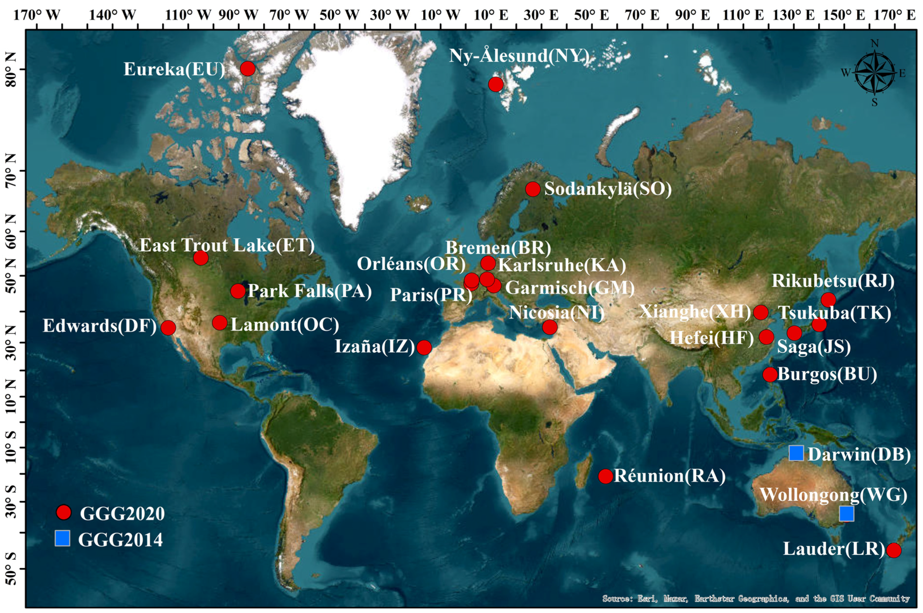
The Global Total Column Carbon Observation Network (TCCON) is a ground-based Fourier Spectrometer (FTS) network that uses the GGG software to retrieve column-averaged mixing ratios of several climate-relevant gases, including CO2, N2O, CH4, and CO, from ground-based solar absorption spectra. TCCON sites adopt continuous observation mode to acquire spectral data, and the data obtained undergo standardized processing resulting in good stability. Compared with its predecessor GGG2014, GGG2020 has several key improvements including changes to the spectroscopic database, prior profiles, spectral fitting, and post processing. The GGG2020 version has evaluated bias budget as less than 0.16% (~0.6 ppm) for observations with a solar zenith angle of less than 82° [22]. As of 2023, the network consists of 28 operational sites, 5 previous sites, and 3 future sites globally. TCCON sites are predominantly distributed in Europe and North America, followed by East Asia (Japan, China), and Oceania. To ensure comprehensive coverage, this paper selected 22 valid sites from the GGG2020 version, along with Darwin and Wollongong from the GGG2014 version, spanning the period from 2019 to 2021. In total, 24 sites were included in the analysis (Figure 1), roughly 2.5 years of TCCON data are included in the research. The location and access dates of these sites are detailed in Table 1.
Ground-based observations, similar to satellite products, also require quality filtering. in the atmosphere typically exhibits daily variations of less than 1 ppm [8], seasonal changes within a few ppm range, annual increases of about 2 ppm to 3 ppm, and regional fluctuations of less than 10 ppm [49]. TCCON sites are required to be built far from emission source in areas where carbon dioxide levels remain relatively stable. Consequently, under normal conditions, there should be no sudden fluctuations in the effective observations of TCCON measurements. The daily change threshold is set at 3 ppm to filter out any anomalous values. Considering the difference in prior distribution and average kernel when observed by different measuring instruments, the research refers to method for column averaging kernel function correction [12]. TCCON divides the atmosphere into 50 layers from 0 to 1000 h Pa, while OCO-2 divides into 20 layers. Typically, it is assumed that the averaging kernel in each pressure layer changes linearly with the pressure. To align the averaging kernel of TCCON and OCO-2, linear interpolation is employed. Additionally, the CO2 prior profile of TCCON is converted into a dry CO2 profile using the prior H2O profile (Equation (1)). Subsequently, the profile correction value is calculated according to the pressure weighting function, the column averaging kernel, and the prior CO2 profiles (Equation (2)). The largest daily average difference before and after the correction amounts to 0.15 ppm.
and are a priori profile of CO2 in dry and wet atmospheres, respectively, is a priori profile of H2O in a wet atmosphere. They are all from one shoot.
is the adjusted CO2 column, is the actual retrieval CO2 column of OCO-2, represents the pressure weight function, is the identity matrix, represents the column averaging kernel of OCO-2, represents the a priori CO2 profile observed by TCCON, and represents OCO-2 a priori CO2 profile after extended interpolation by the layers of TCCON.
2.3. Auxiliary Data
Potential temperature is a stable atmospheric tracer, which demonstrates a notable correlation with the CO2 concentration in the mid-latitudes of the Northern Hemisphere [50]. Previous studies have explored the use of the potential temperature gradient at 700 hPa in the troposphere to establish connections between the GOSAT satellite and TCCON measurements [9,16]. In this paper, we utilized global daily mean tropospheric potential temperature data obtained from the reanalysis product of the National Center for Environmental Prediction and the National Center for Atmospheric Research (NCEP/NCAR). The data have a spatial resolution of 2.5 and are assimilated with historical data through an advanced analysis/forecasting system [51]. In Section 3.2, we introduce the potential temperature of tropospheric T700 as a covariate of longitude, latitude, and time. In this approach, observations with large changes in CO2 are abandoned by filtering observations with large differences in potential temperature within the neighborhood regions.
2.4. Research Methods
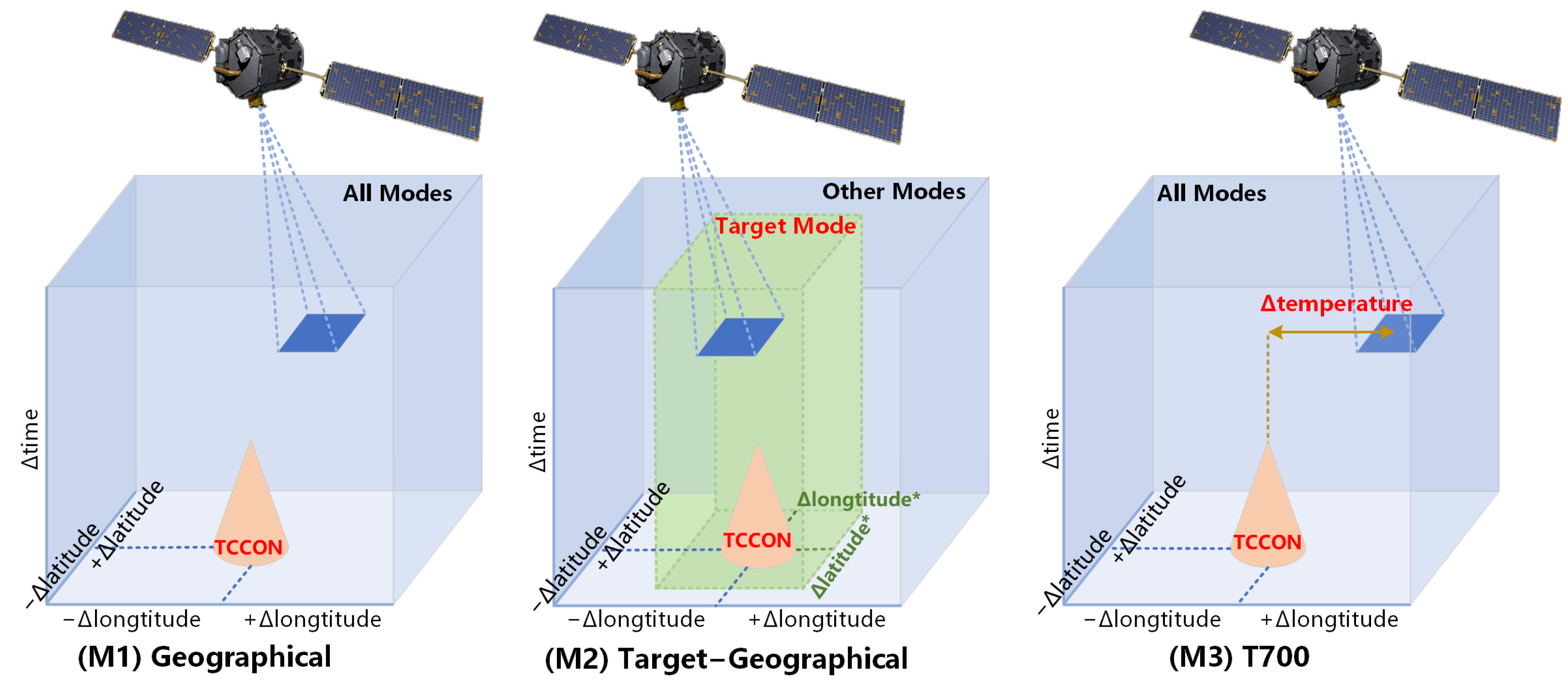
This paper conducted experiments under multiple sets of matching conditions, and analyzed the influence of spatiotemporal neighborhood regions and matching methods on evaluating the bias of TCCON and OCO-2 retrieval products on the principle of controlling variables. Considering factors such as orbital interval and atmospheric heterogeneity, the range of spatial neighborhood was experimented from 1 and 10 (interval 1) to evaluate the influence of the spatial neighborhood on bias and at 30 min, 60 min, and 120 min to evaluate the bias caused by temporal neighborhood. Then, the colocation methods were compared by using the geographical (M1), target-geographical (M2), and T700 (M3) (Figure 2). M1 refers to regard the satellite and ground observations which they are within the geographical constraints () as approximately synchronous observation. M2 imposes stricter conditional constraints for the target observation mode alone on the basis of M1. The instantaneous target observation of OCO-2 needs to be within a narrower spatial window range () to be considered as approximately synchronous observation. M3 entails that while meeting the geographical constraints, it is also necessary to ensure that the T700 potential temperature of OCO-2 and TCCON at the instantaneous position of observation meets the requirements of the distance function. Consequently, each site conducted experiments under 30 sets of distinct conditions, after averaging daily matched observations, considering time and space constraints as independent variables and uncertainties as dependent variables. The bias was quantified using RMSE and correlation coefficients.
represents the retrieval by TCCON, represents the retrieval by OCO-2 which meet the colocation requirement.
3. Results
This paper investigates the bias of OCO-2 and TCCON retrieval products, focusing on the factors of time, spatial neighborhood, and colocation method. Figure 3 illustrates the time series matching results of 24 TCCON sites with OCO-2 under the most relaxed spatiotemporal neighborhood conditions (10/120 min). The observed values from OCO-2 exhibit consistent with TCCON, showing a year-by-year increase. Seasonal pattern is evident in the Northern Hemisphere. The matching results display relatively continuous at mid-latitude sites, but they are missing in time at high-latitude sites (EU, NY). In the Southern Hemisphere, there is obvious deviation between TCCON and OCO-2 observations, characterized by significant underestimation (DB, RA). Compared to Oceania and Africa, TCCON sites located in Europe, Asia, and North America exhibit significantly better consistency with OCO-2 which display high correlation coefficients (>0.9) and reliable uncertainties (close to 1 ppm) on average.
3.1. Influence of Spatiotemporal Neighborhood on Bias
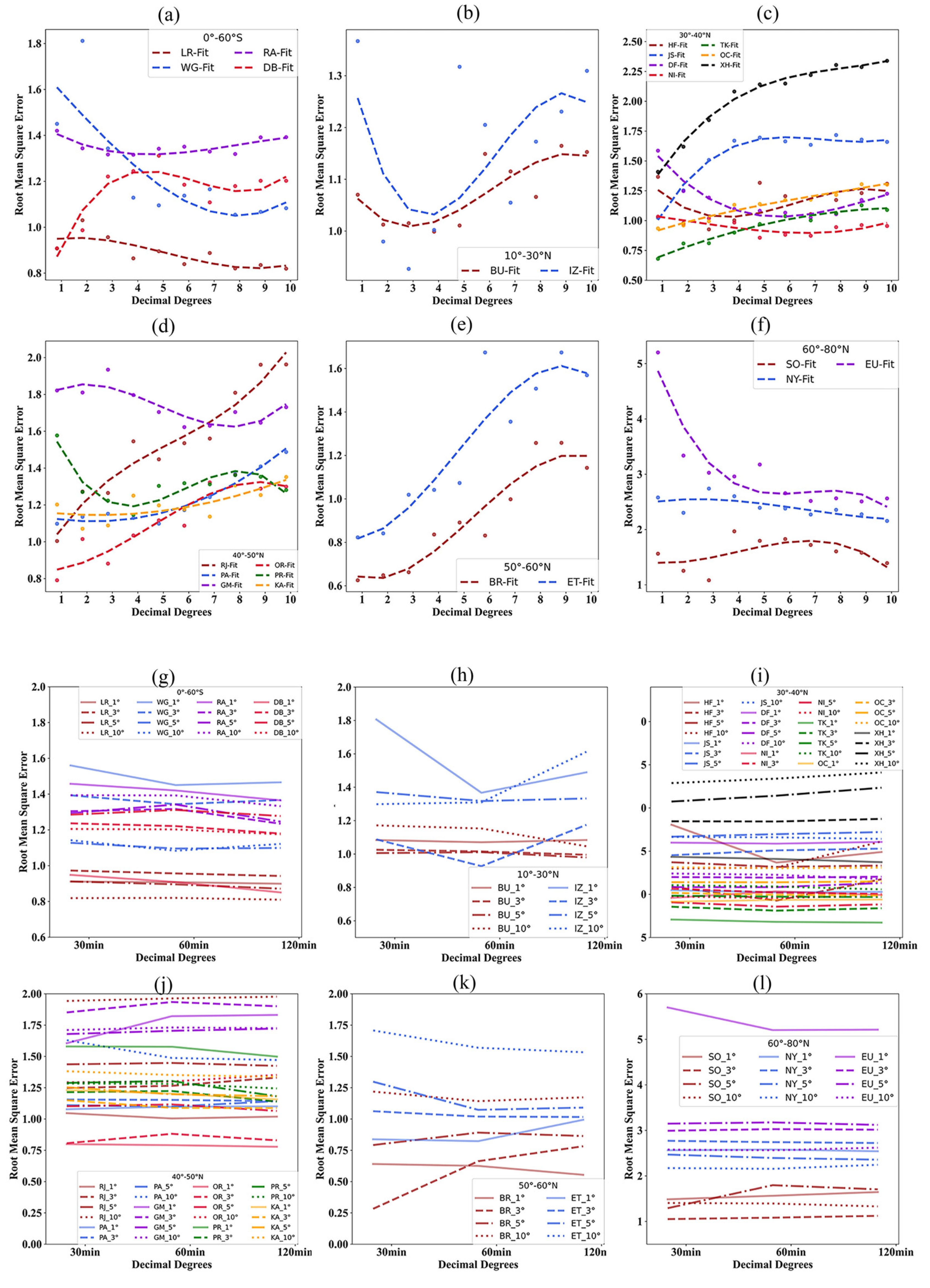
Considering the differences in carbon cycle between the southern and Northern Hemispheres, as well as between mid-latitudes and high-latitudes, this paper divided 24 sites into six groups based on latitude: 0–60S, 10–30N, 3040N, 40–50N, 50–60N, and 60–80N. Figure 4 displays the influence of spatiotemporal neighborhood on evaluating the bias of TCCON and OCO-2.
In the Southern Hemisphere (Figure 4a), the bias of sites and OCO-2 is calculated to be 1.16 0.22 ppm. Among the sites, WG exhibits the largest bias, with a variation of 0.76 ppm in spatial neighborhood.
At low latitudes in the Northern Hemisphere (Figure 4b), the bias of the site initially decreases and then increases as the spatial neighborhood increases. There is a turning point at approximately 3, and the range of variation is relatively small, with a bias of 1.06 0.10 ppm.
In the middle latitudes of the Northern Hemisphere (Figure 4c–e), most sites show an increase in bias with OCO-2 with the increase in the spatial neighborhood. However, there are exceptions to this trend, such as DF located in North America, NI in the Mediterranean coast, and PR and GM in the European continent, which will be further analyzed in Section 4.2. Overall, the bias of the sites at mid-latitudes in the Northern Hemisphere is estimated to be 1.28 0.34 ppm.
At high latitudes in the Northern Hemisphere (Figure 4f), the sites tend to have a higher bias that exhibit more substantial variation with changes in spatial neighborhoods, with a bias of 2.34 0.78 ppm. This increased bias can be attributed to the low reflectivity of snow and ice surfaces in high latitudes in the 1.61 and 2.06 µm bands, leading to greater bias introduced by the scattering of thin clouds and aerosols [16]. As a result, the observations of OCO-2 are continuously missing for several months every year, especially with a limited number of days with matching observations from EU sites, accounting for less than one-tenth of the year.
The bias between high-latitude sites and OCO-2 tends to decrease as the spatial window increases. This trend is shown for sites such as SO, NY, EU in the Northern Hemisphere (Figure 4f) and LR, WG in the Southern Hemisphere (Figure 4a).
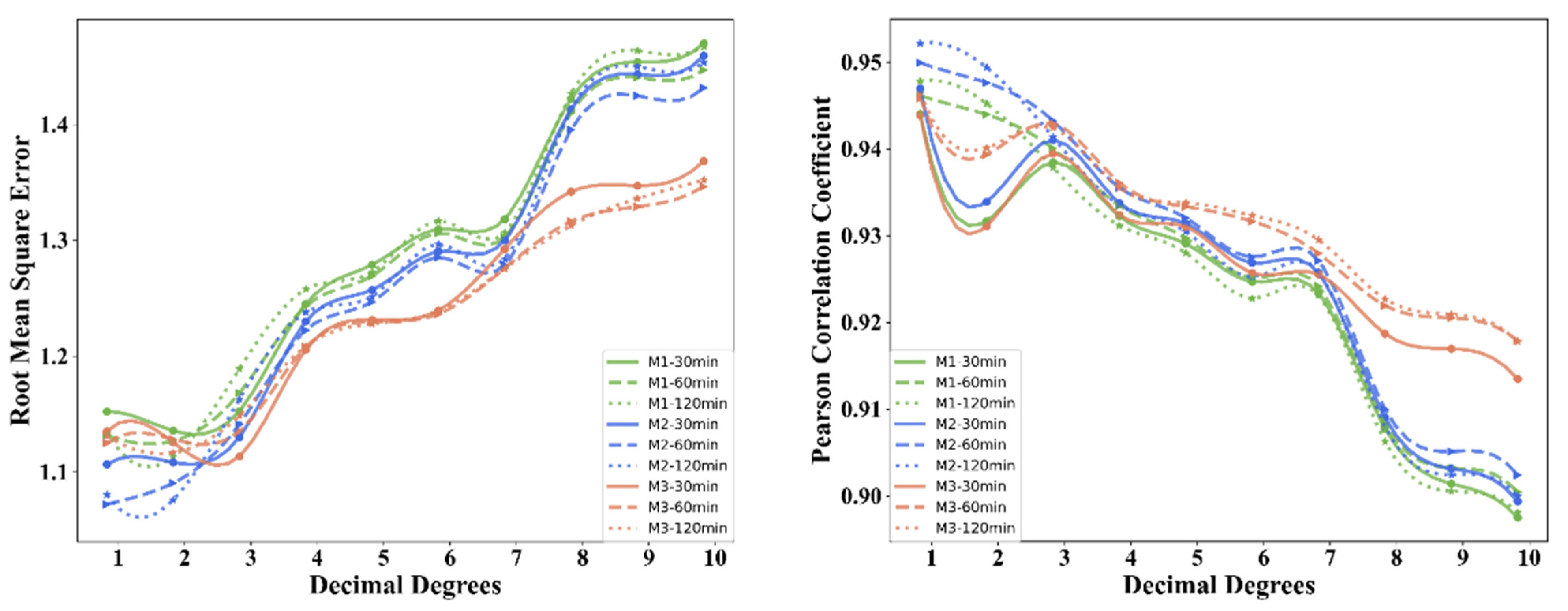
In contrast, the influence of temporal neighborhood is significantly smaller. Most of the trend lines in Figure 4g–l remains approximately horizontal, indicating little to no change with increasing temporal neighborhood. This suggests that the time variability for TCCON and OCO-2 bias is minimal, and therefore, the impact of the temporal neighborhood can be disregarded. TCCON, under normal operating conditions, observes multiple times per minute and continuously observes for a long time during the day. In theory, as long as OCO-2 falls within a reasonable spatial neighborhood, it can be matched with TCCON. Hence, the requirements for spatial neighborhood are more crucial than those for temporal neighborhood.
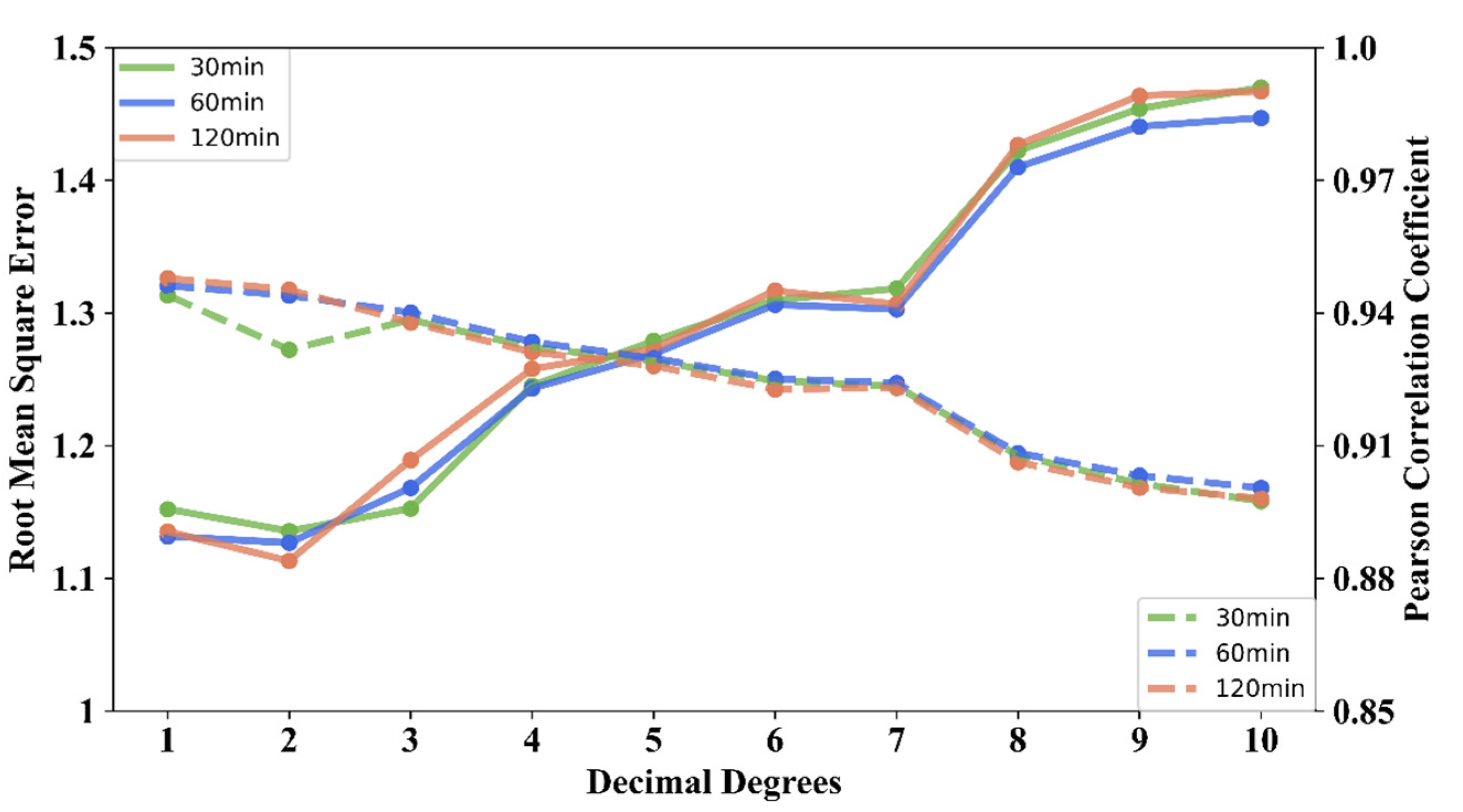
The regularity of mid-latitude stations in the Northern Hemisphere demonstrates much stronger. In the overall trend (Figure 5), as the spatial neighborhood changes from 1 to 10, there is an average decrease of 0.04 in the correlation between TCCON and OCO-2, an average increase of 0.32 ppm in the RMSE, and at least a 28% increase in bias. The impact of temporal neighborhoods has a weaker effect in comparison. To quantitatively assess the degree of influence of the independent variable on the dependent variable, the standardized partial regression coefficient (Beta value) is used. Among them, the Beta values of the correlation coefficient and the spatial neighborhood are −0.56, while the Beta values of the correlation coefficient and the temporal neighborhood are −0.28, both indicating a negative influence. The Beta values of RMSE and the spatial neighborhood are 0.33, while the Beta values of RMSE and the temporal neighborhood are 0.28, both are positive influences. In contrast, the spatial neighborhood exhibits a higher degree of influence on the bias, indicating the bias resulting from the spatiotemporal matching condition is more dependent on the constraints of the spatial neighborhood.
3.2. Influence of Colocation Methods on Bias
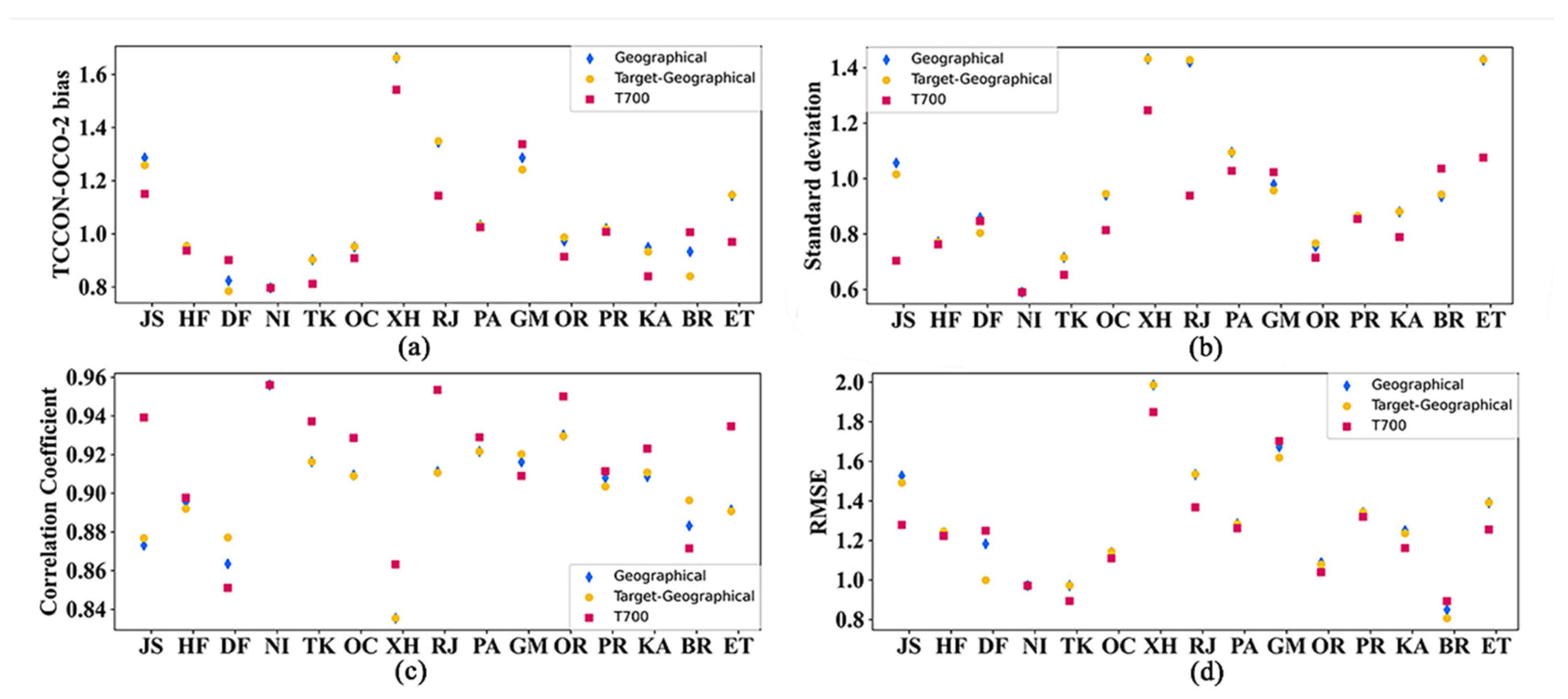
The average statistics of each colocation methods in varying spatiotemporal neighborhoods of the 15 mid-latitude sites in the Northern Hemisphere is shown in Figure 6. The deviations between the site and OCO-2 under three methods is consistent, ranging from 0.80 ppm to 1.70 ppm (Figure 6a). T700 tends to less bias, while Geographical and Target-Geographical produce similar bias. However, the biases of XH and BR site are not reduced significantly with the introduction of potential temperature gradients (Figure 6a,b). This could be due to the limited number of matched observations, resulting in less robust bias estimates. The correlation coefficient (Figure 6c) reflects the goodness of fit between TCCON and OCO-2, and is generally expected to approach 1 to indicate a better fit. Overall, the performance of T700 better than that of Target-Geographical, and they are both better than Geographical. This improvement may be attributed to the strong free tropospheric potential temperature-related gradient in the middle latitude of the Northern Hemisphere [16]. RMSE directly compares the performance of the three methods (Figure 6d). On average, the average RMSE of the T700 method is the lowest, and Geographical and Target-Geographical are similar. Notably, at the JS site, the T700 method reduces the RMSE by 0.25 ppm, resulting in a 16% reduction in bias.
Figure 7 illustrates the average trend of three methods. The performance of each methods shows a positive correlation between the range of the spatial window and the bias, with consistent fluctuation curves. For narrower spatiotemporal neighborhoods (within 3), The Target-Geographical yields lower uncertainties. Between 3 to 10, the superiority of the T700 method becomes gradually evident and more pronounced as the spatial neighborhood increases. The RMSE of the T700 method is reduced by 0.07 0.03 ppm (Geographical) and 0.05 0.04 ppm (Target-Geographical), indicating that the T700 method effectively mitigates the bias stemming from the spatial neighborhood. This conclusion is further quantitatively explained by the linear relationship that the RMSE of the three methods increases by 0.040 ppm, 0.044 ppm and 0.029 ppm for every 1 increase in the spatial neighborhood.
4. Discussion
4.1. Spatiotemporal Colocation under Low Satellite Coverage
Theoretically, employing a strict colocation method and a narrow spatiotemporal neighborhood can decrease the bias of TCCON and OCO-2 measurements. However, this approach reduces the number of matching observations and hindering the evaluation of accuracy and model correction due to poor time continuity. As the spatiotemporal neighborhood expands, the number of observations matches increases, but the bias also increases based on the results of Section 2. The study found that for sites located in the middle latitudes of the Northern Hemisphere, opting for a stricter spatiotemporal neighborhood in the Geographical method results in lower uncertainties, but sacrifices an average of 26% of the number of observations. Conversely, selecting a more relaxed spatiotemporal neighborhood for more matching data, but introduces an average bias increase of 0.40 ppm. The decision of which approach to adopt has a significant impact, particularly for sites with low satellite observation coverage like HF, BR, RA, and PR, as well as high-latitude NY and SO (Figure 3).
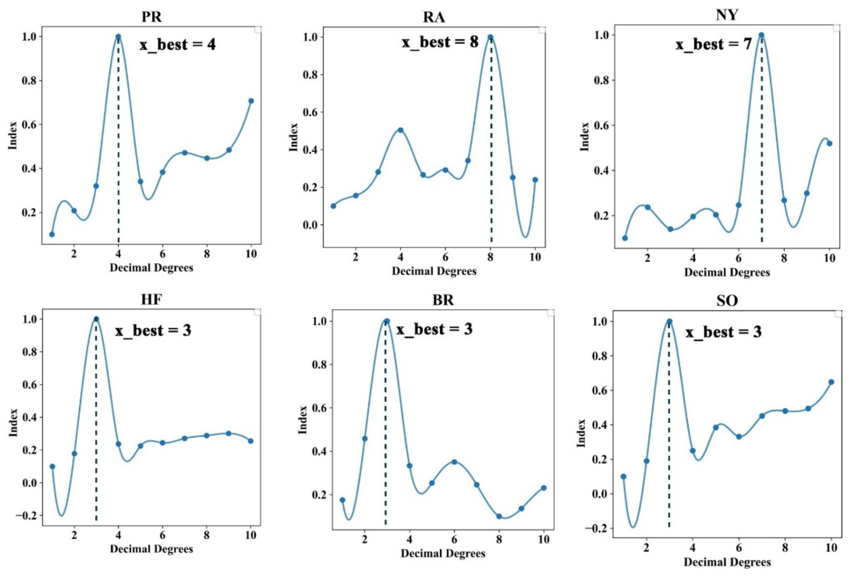
The study defined a simple PQ index to characterize the influence of spatial neighborhood on accuracy and number of observations in colocation. The PQ index represents the percentage of matching number and RMSE, with all data standardized. The site with low satellite coverage were found to exhibit a curve that closely resembles a partial normal distribution (Figure 8). In this curve, the x-axis value corresponding to the maximum point is considered the optimal spatial window, denoted as “x_best”. This value represents the balance between accuracy and the number of observations.
The utilization of the PQ index and the determination of the optimal spatial window can serve as a reference for selecting matching conditions for sites with low satellite coverage. It provides a means to strike a balance between accuracy and the availability of observations, enabling the selection of an appropriate spatiotemporal neighborhood that optimizes the performance of colocation methods at these sites. Under the premise of ensuring bias, with as many satellite observations as possible, this method may provide a reference for selecting matching conditions for sites with low satellite coverage.
4.2. Bias Distribution of TCCON and OCO-2
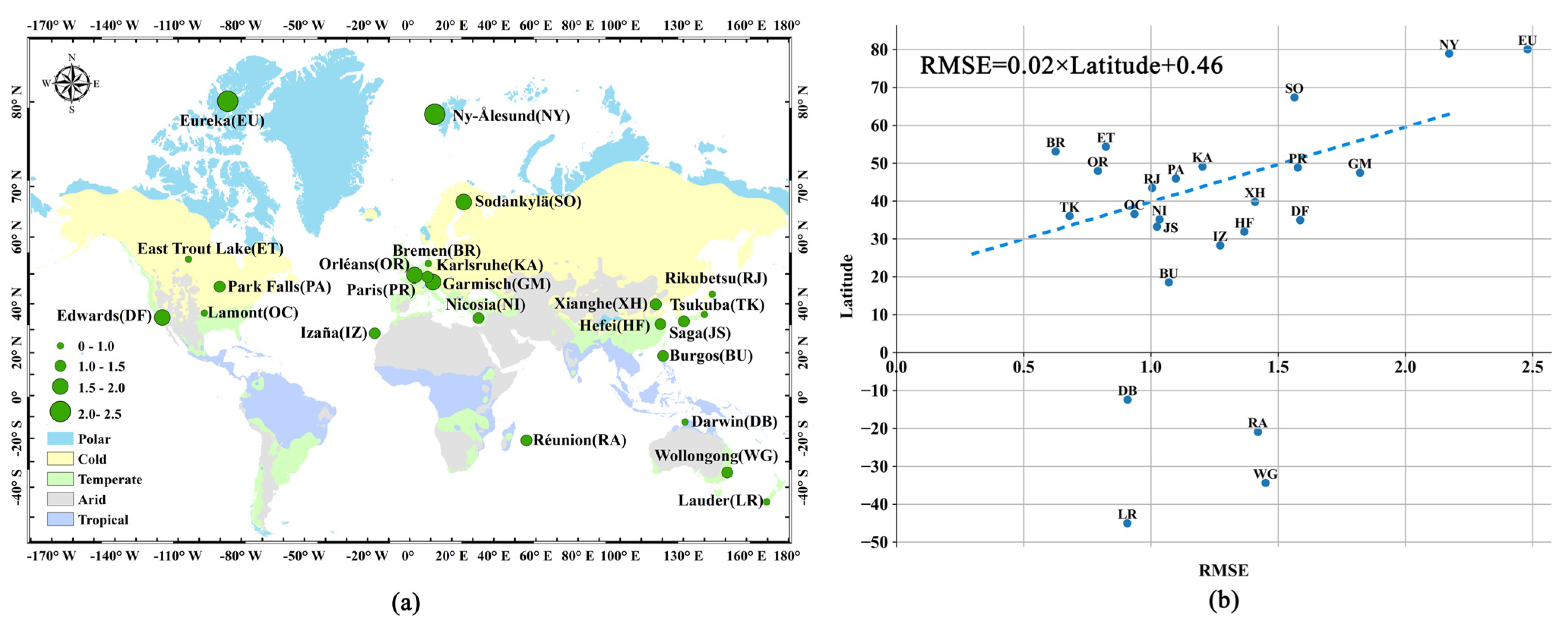
The spatial distribution of TCCON and OCO-2 uncertainties has a direct impact on the ability of satellite regional monitoring applications. In Figure 9a, the bias distribution of 24 sites and OCO-2 is depicted, covering a latitude range from 50°S to 80°N (the neighborhood region considered is 1°). It can be observed that as the latitude zone increases, the bias of ground-based and satellite products increases. Figure 9b also shows such results, the correlation between the latitude and bias of Northern Hemisphere stations reaches 0.64 (significant at the p < 0.01 level). For every 10 increase in latitude, there is an associated 0.20 ppm (16%) increase in bias. These results indicate that higher latitudes are more likely to have increased uncertainties between ground-based and satellite measurements. The observed correlation suggests that there may be underlying factors related to latitude that contribute to the increase in bias. Understanding and accounting for these factors becomes important when using satellite data for regional monitoring applications, particularly at higher latitudes.
Compared to sites at the same latitude discussed in Section 3, DF and GM do not exhibit the expected behavior. TCCON sites undergo a rigorous site selection process, ensuring that human activities within 100 km have minimal impact, and the land conditions in these areas have remained relatively unchanged for decades. The neighborhood of OCO-2 we define is also within this range. It is reasonable to assume that TCCON and OCO-2 should observe the similar value in the neighborhood. Then, the natural factor causing the bias becomes the difference of air masses. We attempt to use natural winds to explain why DF and GM perform worse due to the different air masses observed by OCO-2. Directionality is a characteristic of wind, and the research focuses on characterizing the bias in the direction of matching the effect of wind at the position of TCCON at the time of observation. When the wind direction is nondominant and the wind speed is weak, slow atmospheric transport can lead to local CO2 accumulation. Conversely, when the dominant wind speed is high, it facilitates atmospheric transport, resulting in varying impacts on TCCON sites depending on the underlying surfaces characteristics. Therefore, the effect of natural wind will lead to differences in the satellite–ground observations in neighborhoods.
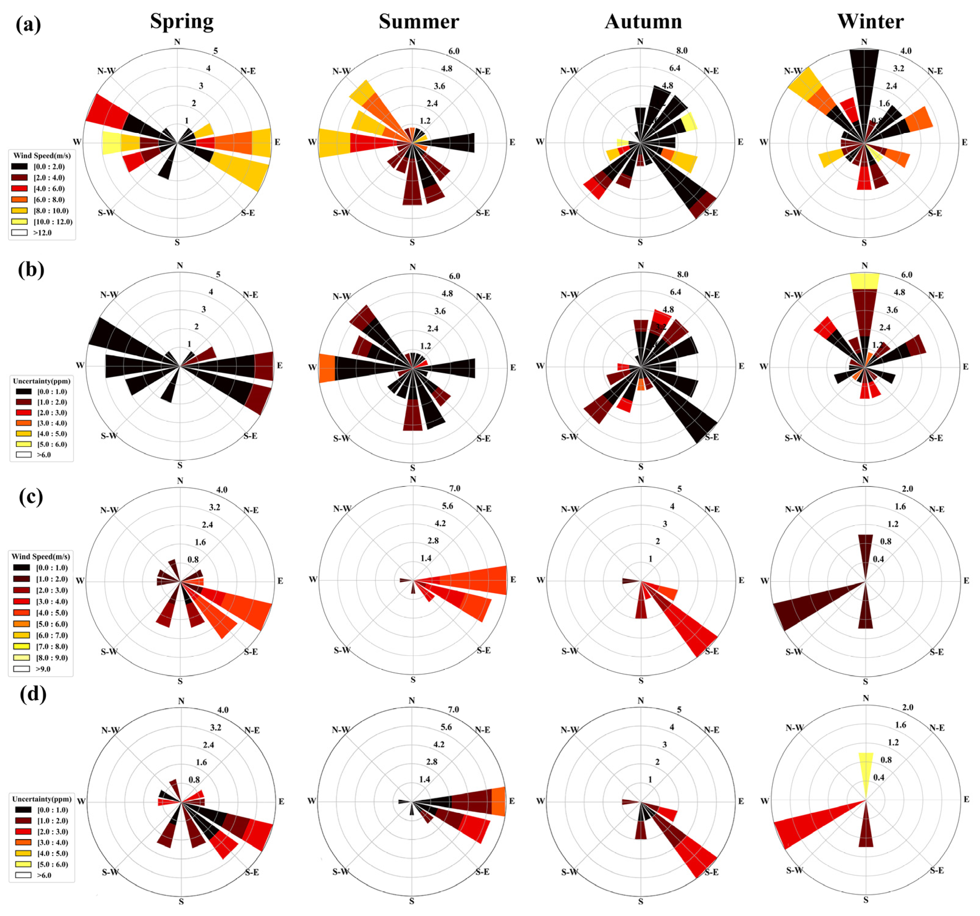
We combined the local climate and geographical environment, taking the DF and GM in the Northern Hemisphere as examples to explore the differences between TCCOM and OCO-2 uncertainties in different directions. The uncertainties at 16 azimuths are analyzed for site and OCO-2 observations that satisfy the spatiotemporal window (Figure 10b,d), and the wind direction and speed of the surface wind at this time are drawn as a rose diagram (Figure 10a,c).
DF, located in the southwest of California, USA, falls within a desert climate and semi-arid climate region. The sparse vegetation coverage on the underlying surface contributes to the accumulation of local CO2 concentration, which reached 420 ppm in June 2020. However, the average annual observed concentration at DF sites in 2020 was 412.80 ppm, lower than the global average, which was 413.20 ppm in the same year. This suggests that active atmospheric transport plays a role in CO2 exchange at the site.
DF is positioned to the west of the Rocky Mountains and close to the Pacific coast. The prevailing northeast trade wind blows from the Pacific inland throughout the year, with peak intensity from March to July. Consequently, there is a significant contrast in DF between the sea–land direction and the coastline direction. The annual average bias of DF and OCO-2 in the sea–land direction is 1.72 ppm, which in the coastline direction is 1.09 ppm. The wind rose diagram (Figure 10a,b) shows the wind field of DF when OCO-2 is approximately passing through. In the diagram, the color bands from black, to red, to yellow represent increasing values. While there is no strict causal relationship between wind speed and bias, it is observed that biases tend to occur more frequently in directions with higher wind speed. In spring, when OCO-2 is in the vicinity of DF, the prevailing wind direction is east–west. The frequency of wind in the ENE–E–ESE direction is 43%, with an average wind speed is 5.8 m s−1. High bias values are more likely to occur when the wind speed exceeds 8 m s−1, reaching up to 1.8 ppm. In the direction of WNW–W–WSW, which accounts for 43% of the wind frequency, the bias is relatively lower. In summer, the dominant wind direction is NW–WNW–W, with an average wind speed of 7 m s−1. High bias values occurs when the wind speed exceeds 9 m s−1, with an average of 1.9 ppm. During autumn, the wind direction is complex, and the average wind speed is relatively low, and the relationship is not as apparent. In winter, the dominant wind direction comes from NW–N–ENE, accounting for 57%. When the wind speed exceeds 3 m s−1, the average bias is 2.1 ppm.
GM is located in Bavaria, Germany, at the junction of alpine, oceanic, and subtropical humid climate. Its proximity to the Mediterranean Sea exposes it to the alternating circulation of pressure belts and wind belts. The bias in the east–west direction, which corresponds to the junction of these climatic zones, averages at 2.44 ppm, while the bias in the north–south direction is about 1.82 ppm. The perennial zonal wind is generally stronger than the radial wind (Figure 10c). This could explain why the bias in the latitudinal direction is higher compared to the radial direction at GM. For instance, the dominant wind in spring is ESE–SE–SSE. When the bias exceeds 1 ppm, higher wind speeds in these directions tend to correspond to greater uncertainties. During summer and autumn, the high values of bias primarily occur when the wind speed exceeds 3 m s−1.
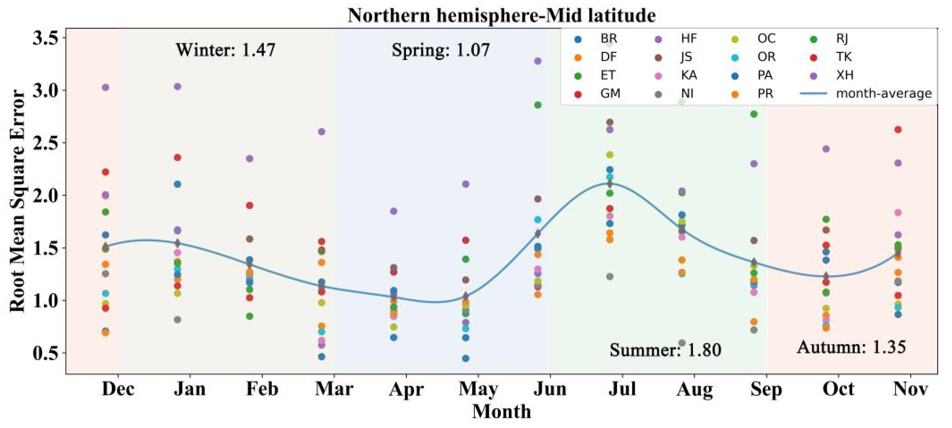
4.3. Seasonality of TCCON and OCO-2 Bias
Seasonal variations in atmospheric CO2 are influenced by both local and global carbon cycles. The exchange of CO2 between the atmosphere and the terrestrial biosphere in the Northern Hemisphere plays a large role in seasonal variation. This is because the growth of terrestrial vegetation follows a seasonal pattern, regulating the carbon exchange with the atmosphere. Additionally, a large portion of the global landmass is situated north of 30°N (43%, excluding Antarctica), leading to a characteristic pattern of CO2 decrease in summer and increase in winter [52]. In our results, we also observe a pronounced seasonality in the bias of TCCON and OCO-2 measurements within 10°. Generally, the bias shows a gradual decline during winter, reaching its lowest point in the months of March to May. It then increases during spring, peaks in July during summer, and subsequently declines towards autumn (Figure 11). The seasonal representation of bias in ground observations and satellite products is influenced by variations in the atmospheric state throughout the year and seasonal variations in the accuracy of satellite inversion algorithms. Climate patterns in summer such as active pressure belts or monsoon circulations can lead to increased CO2 exchange between the land and atmosphere due to the activation of terrestrial ecosystems. In the same spatiotemporal neighborhood, the relatively unstable atmospheric state contributes to increased bias in satellite–ground observations. However, when the colocation range becomes small (3°), seasonality is less pronounced.
5. Conclusions
The combination of ground and satellite observations is performed by interpolating nearby satellite measurements to estimate what the ground perceive at the same spatiotemporal coordinates. This process is crucial for further evaluating and validating the instruments and algorithms used in satellite observations. However, satellite observations rarely coincide with ground observations absolutely in time and space. Moreover, the method of constructing satellite–ground spatiotemporal links will introduce errors. Therefore, the quantitative significance of collocating on satellite product validation will be more important for CO2 satellite retrieval with higher resolution and higher accuracy in the future. Our research is to quantitatively describe the influence of spatiotemporal neighborhood and colocation methods on the bias of satellite–ground retrieval products. The results show that spatial neighborhoods exert a more substantial influence on bias compared to temporal neighborhoods. In the mid-latitudes of the Northern Hemisphere, the influence of temporal and spatial neighborhoods on bias exhibits a negative relationship. As the spatial neighborhood changes from 1 to 10, the observed difference between OCO-2 and TCCON shows an approximately linear increase trend. The average increase is 0.32 ppm, which is meaningful for enhancing the CO2 retrieval accuracy (current is 0.25% [6]). Regarding colocation methods, the simple spatiotemporal geographic constraints tend to overlook changes in the atmospheric state to a certain extent. Meanwhile, the target geographic constraint method reduces the bias by 2% to 5% by increasing the proportion of OCO-2 observations targeting TCCON and the method of introducing T700 potential temperature reduces the bias by 2 to 13% by screening the gradient of CO2 concentration change.
The global distribution of TCCON and OCO-2 uncertainties directly influence the suitability of satellite products for regional monitoring applications. An evident correlation exists between the bias in the Northern Hemisphere and their corresponding latitudes, with a 0.2 ppm increase in bias observed for every 10° increment in latitudes. For the special sites of DF and GM, an analysis was conducted to attribute the observed uncertainties to wind field factors. It is evident that wind direction with high annual wind speed of site location, such as the direction of sea and land and the direction of climate zone change, the bias is higher. Natural wind jointly affects the atmospheric state above TCCON and below OCO-2 observations and the inversion process. While there is currently a lack of quantitative results directly linking natural wind to bias, it remains a topic worthy of exploration. It is important to recognize that the factors contributing to natural CO2 variations extend beyond the influence of natural wind. In this part of study, we regard the influence of natural wind on the colocation bias as the influence of natural factors, which is insufficient.
The retrieval of CO2 from satellite observations is obtained within the constraints of various spatiotemporal variables, and it is important to note that the concentrations of CO2 in the free troposphere and at the surface exhibit significant differences [53]. Therefore, the discrepancies between TCCON and satellite observations are multifaceted and complex. In addition, TCCON sites situated in mid-latitude, the distribution of CO2 is largely influenced by weather variations acting on large-scale gradients, which complicates the question of whether sparse measurements are representative of larger regions [50]. Therefore, the general patterns and rules derived from categorization might not be universally applicable to sites situated at different latitudes, within diverse climate zones, and under varying weather conditions. The uniqueness of low latitudes, high latitudes, and the Southern Hemisphere warrants careful consideration and may require specific considerations distinct from those applicable to mid-latitudes.
The bias of TCCON and OCO-2 shows a pronounced seasonal regularity, with the highest in summer. This seasonal pattern can be attributed to natural factors, such as active land–atmosphere exchange and monsoon circulation in summer, which lead to satellite retrieval errors in summer being higher than in winter. In fact, the bias of OCO-2 retrieval is influenced by multiple factors, including smoothing errors resulting from the correlation of inversion parameters, noise errors arising from sensor random noise, and interference errors caused by the unintegrated parameters, among which the most influential factors are aerosols, surface coverage, surface pressure, and surface albedo. TCCON products also have uncertainties in instruments and retrieval models. Therefore, the bias discussed in this paper represents a comprehensive representation of both the natural variability and the bias in the two retrieval algorithms. Subsequent attempts may be made to explore the reason from the perspective of retrieval model for the influence of colocation on bias.
Author Contributions
Conceptualization, X.Z., T.C., and X.G.; methodology, R.L., Z.T., and N.W.; software, R.L.; validation, Z.T. and R.L.; formal analysis, R.L.; investigation, R.L. and H.Z.; writing—original draft preparation, R.L.; writing—review and editing, Z.T. and N.W.; visualization, R.L.; supervision, X.Z. and T.L.; project administration, H.Z.; funding acquisition, T.C. All authors have read and agreed to the published version of the manuscript.
Funding
This research was funded by the National Key R&D Program of China (grant nos. 2022YFB3904801).
Data Availability Statement
Not applicable.
Acknowledgments
This research was supported by Land Observation Satellite Supporting Platform of National Civil Space Infrastructure Project. NCEP/NCAR data were obtained from the Copernicus Data Store (https://apps.ecmwf.int/data-catalogues/era5/, accessed on 7 February 2023). OCO-2 data were obtained from NASA (https://disc.gsfc.nasa.gov/, accessed on 4 January 2023). TCCON data were obtained at Caltech Library Research Data Repository (https://tccondata.org/, accessed on 25 August 2022). Thanks to all the authors of the atmospheric remote sensing field study.
Conflicts of Interest
The authors declare no conflict of interest.
References
- Sixth Assessment Report-IPCC. Available online: https://www.ipcc.ch/assessment-report/ar6/ (accessed on 10 September 2022).
- Gruber, N.; Gloor, M.; Mikaloff Fletcher, S.E.; Doney, S.C.; Dutkiewicz, S.; Follows, M.J.; Gerber, M.; Jacobson, A.R.; Joos, F.; Lindsay, K.; et al. Oceanic sources, sinks, and transport of atmospheric CO2. Glob. Biogeochem. Cycles 2009, 23, GB1005. [Google Scholar] [CrossRef]
- Fung, I.Y.; Doney, S.C.; Lindsay, K.; John, J. Evolution of carbon sinks in a changing climate. Proc. Natl. Acad. Sci. USA 2005, 102, 11201–11206. [Google Scholar] [CrossRef] [PubMed]
- Friedlingstein, P.; Cox, P.; Betts, R.; Bopp, L.; von Bloh, W.; Brovkin, V.; Cadule, P.; Doney, S.; Eby, M.; Fung, I.; et al. Climate–Carbon Cycle Feedback Analysis: Results from the C4MIP Model Intercomparison. J. Clim. 2006, 19, 3337–3353. [Google Scholar] [CrossRef]
- Washenfelder, R.A.; Toon, G.C.; Blavier, J.F.; Yang, Z.; Allen, N.T.; Wennberg, P.O.; Vay, S.A.; Matross, D.M.; Daube, B.C. Carbon dioxide column abundances at the Wisconsin Tall Tower site. J. Geophys. Res. 2006, 111, D22305. [Google Scholar] [CrossRef]
- Wunch, D.; Toon, G.C.; Blavier, J.F.; Washenfelder, R.A.; Notholt, J.; Connor, B.J.; Griffith, D.W.; Sherlock, V.; Wennberg, P.O. The total carbon column observing network. Philos. Trans. A Math. Phys. Eng. Sci. 2011, 369, 2087–2112. [Google Scholar] [CrossRef]
- Chevallier, F.; Bréon, F.-M.; Rayner, P.J. Contribution of the Orbiting Carbon Observatory to the estimation of CO2 sources and sinks: Theoretical study in a variational data assimilation framework. J. Geophys. Res. 2007, 112, D09307. [Google Scholar] [CrossRef]
- Olsen, S.C. Differences between surface and column atmospheric CO2 and implications for carbon cycle research. J. Geophys. Res. 2004, 109, D02301. [Google Scholar] [CrossRef]
- Nguyen, H.; Osterman, G.; Wunch, D.; O’Dell, C.; Mandrake, L.; Wennberg, P.; Fisher, B.; Castano, R. A method for colocating satellite XCO2 data to ground-based data and its application to ACOS-GOSAT and TCCON. Atmos. Meas. Tech. 2014, 7, 2631–2644. [Google Scholar] [CrossRef]
- Cogan, A.J.; Boesch, H.; Parker, R.J.; Feng, L.; Palmer, P.I.; Blavier, J.F.L.; Deutscher, N.M.; Macatangay, R.; Notholt, J.; Roehl, C.; et al. Atmospheric carbon dioxide retrieved from the Greenhouse gases Observing SATellite (GOSAT): Comparison with ground-based TCCON observations and GEOS-Chem model calculations. J. Geophys. Res. Atmos. 2012, 117, D21301. [Google Scholar] [CrossRef]
- Reuter, M.; Bosch, H.; Bovensmann, H.; Bril, A.; Buchwitz, M.; Butz, A.; Burrows, J.P.; O’Dell, C.W.; Guerlet, S.; Hasekamp, O.; et al. A joint effort to deliver satellite retrieved atmospheric CO2 concentrations for surface flux inversions: The ensemble median algorithm EMMA. Atmos. Chem. Phys. 2013, 13, 1771–1780. [Google Scholar] [CrossRef]
- Inoue, M.; Morino, I.; Uchino, O.; Miyamoto, Y.; Yoshida, Y.; Yokota, T.; Machida, T.; Sawa, Y.; Matsueda, H.; Sweeney, C.; et al. Validation of XCO2 derived from SWIR spectra of GOSAT TANSO-FTS with aircraft measurement data. Atmos. Chem. Phys. 2013, 13, 9771–9788. [Google Scholar] [CrossRef]
- Guerlet, S.; Butz, A.; Schepers, D.; Basu, S.; Hasekamp, O.P.; Kuze, A.; Yokota, T.; Blavier, J.F.; Deutscher, N.M.; Griffith, D.W.T.; et al. Impact of aerosol and thin cirrus on retrieving and validating XCO2 from GOSAT shortwave infrared measurements. J. Geophys. Res. Atmos. 2013, 118, 4887–4905. [Google Scholar] [CrossRef]
- Wunch, D.; Wennberg, P.O.; Osterman, G.; Fisher, B.; Naylor, B.; Roehl, C.M.; O’Dell, C.; Mandrake, L.; Viatte, C.; Kiel, M.; et al. Comparisons of the Orbiting Carbon Observatory-2 (OCO-2) measurements with TCCON. Atmos. Meas. Tech. 2017, 10, 2209–2238. [Google Scholar] [CrossRef]
- Liang, A.; Gong, W.; Han, G.; Xiang, C. Comparison of Satellite-Observed XCO2 from GOSAT, OCO-2, and Ground-Based TCCON. Remote Sens. 2017, 9, 1033. [Google Scholar] [CrossRef]
- Wunch, D.; Wennberg, P.O.; Toon, G.C.; Connor, B.J.; Fisher, B.; Osterman, G.B.; Frankenberg, C.; Mandrake, L.; O’Dell, C.; Ahonen, P.; et al. A method for evaluating bias in global measurements of CO2 total columns from space. Atmos. Chem. Phys. 2011, 11, 12317–12337. [Google Scholar] [CrossRef]
- Bovensmann, H.; Burrows, J.P.; Buchwitz, M.; Frerick, J.; Noël, S.; Rozanov, V.V.; Chance, K.V.; Goede, A.P.H. SCIAMACHY: Mission objectives and measurement modes. J. Atmos. Sci. 1999, 56, 127–150. [Google Scholar] [CrossRef]
- Yokota, T.; Oguma, H.; Morino, I.; Inoue, G. A nadir looking SWIR sensor to monitor CO2 column density for Japanese GOSAT project. In Proceedings of the Twenty-Fourth International Symposium on Space Technology and Science, Japan Society for Aeronautical and Space Sciences and ISTS, Miyazaki, Japan, 30 May–6 June 2004; pp. 887–889. [Google Scholar]
- Crisp, D. Measuring Atmospheric Carbon Dioxide from Space with the Orbiting Carbon Observatory-2 (OCO-2). In Proceedings of the Earth Observing Systems, San Diego, CA, USA, 8 September 2015. [Google Scholar]
- Eldering, A.; Taylor, T.E.; O’Dell, C.W.; Pavlick, R. The OCO-3 mission: Measurement objectives and expected performance based on 1 year of simulated data. Atmos. Meas. Tech. 2019, 12, 2341–2370. [Google Scholar] [CrossRef]
- Crisp, D.; Atlas, R.M.; Breon, F.M.; Brown, L.R.; Burrows, J.P.; Ciais, P.; Connor, B.J.; Doney, S.C.; Fung, I.Y.; Jacob, D.J.; et al. The Orbiting Carbon Observatory (OCO) mission. Adv. Space Res. 2004, 34, 700–709. [Google Scholar] [CrossRef]
- Laughner, J.L.; Toon, G.C.; Mendonca, J.; Petri, C. The Total Carbon Column Observing Network’s GGG2020 Data Version. Earth Syst. Sci. Data, 2023; in review. [Google Scholar] [CrossRef]
- Pollard, D.; Robinson, J.; Shiona, H. TCCON Data from Lauder (NZ), Release GGG2020.R0; TCCON Data Archive, Hosted by CaltechDATA; California Institute of Technology: Pasadena, CA, USA, 2022. [Google Scholar] [CrossRef]
- Sherlock, V.; Connor, B.; Robinson, J.; Shiona, H.; Smale, D.; Pollard, D. TCCON Data from Lauder, New Zealand, 125HR, Release GGG2020R0; TCCON Data Archive, Hosted by CaltechDATA; California Institute of Technology: Pasadena, CA, USA, 2022. [Google Scholar] [CrossRef]
- Sherlock, V.; Connor, B.; Robinson, J.; Shiona, H.; Smale, D.; Pollard, D. TCCON Data from Lauder, New Zealand, 120HR, Release GGG2020R0; TCCON Data Archive, Hosted by CaltechDATA; California Institute of Technology: Pasadena, CA, USA, 2022. [Google Scholar] [CrossRef]
- Griffith, D.W.T.; Velazco, V.A.; Deutscher, N.M.; Murphy, C.; Jones, N.; Wilson, S.; Macatangay, R.; Kettlewell, G.; Buchholz, R.R.; Riggenbach, M. TCCON Data from Wollongong (AU), Release GGG2014R0; California Institute of Technology: Pasadena, CA, USA, 2014. [Google Scholar] [CrossRef]
- Maziere, D.; Sha, M.K.; Desmet, F.; Hermans, C.; Scolas, F.; Kumps, N.; Zhou, M.; Metzger, J.-M.; Duflot, V.; Cammas, J.-P. TCCON Data from Reunion Island (La Reunion), France, Release GGG2020R0; TCCON Data Archive, Hosted by CaltechDATA; California Institute of Technology: Pasadena, CA, USA, 2022. [Google Scholar] [CrossRef]
- Griffith, D.W.T.; Deutscher, N.M.; Velazco, V.A.; Wennberg, P.O.; Yavin, Y.; Aleks, G.K.; Washenfelder, R.A.; Toon, G.C.; Blavier, J.-F.; Murphy, C.; et al. TCCON Data from Darwin (AU), Release GGG2014R0; California Institute of Technology: Pasadena, CA, USA, 2014. [Google Scholar] [CrossRef]
- Morino, I.; Velazco, V.A.; Hori, A.; Uchino, O.; Griffith, D.W.T. TCCON Data from Burgos, Philippines, Release GGG2020R0; TCCON Data Archive, Hosted by CaltechDATA; California Institute of Technology: Pasadena, CA, USA, 2022. [Google Scholar] [CrossRef]
- Blumenstock, T.; Hase, F.; Schneider, M. TCCON Data from Izana, Tenerife, Spain, Release GGG2020R0; TCCON Data Archive, Hosted by CaltechDATA; California Institute of Technology: Pasadena, CA, USA, 2022. [Google Scholar] [CrossRef]
- Liu, C.; Wang, W.; Sun, Y.; Shan, C. TCCON Data from Hefei, China, Release GGG2020R0; TCCON Data Archive, Hosted by CaltechDATA; California Institute of Technology: Pasadena, CA, USA, 2022. [Google Scholar] [CrossRef]
- Shiomi, K.; Kawakami, S.; Ohyama, H.; Arai, K.; Okumura, H.; Ikegami, H.; Usami, M. TCCON Data from Saga, Japan, Release GGG2020R0; TCCON Data Archive, Hosted by CaltechDATA; California Institute of Technology: Pasadena, CA, USA, 2022. [Google Scholar] [CrossRef]
- Iraci, L.; Podolske, J.; Roehl, C.; Wennberg, P.O.; Blavier, J.-F.; Allen, N.; Wunch, D.; Osterman, G. TCCON Data from Armstrong Flight Research Center, Edwards, CA, USA, Release GGG2020R0; TCCON Data Archive, Hosted by CaltechDATA; California Institute of Technology: Pasadena, CA, USA, 2022. [Google Scholar] [CrossRef]
- Petri, C.; Vrekoussis, M.; Rousogenous, C.; Warneke, T.; Sciare, J.; Notholt, J. TCCON Data from Nicosia, Cyprus, Release GGG2020R0; TCCON Data Archive, Hosted by CaltechDATA; California Institute of Technology: Pasadena, CA, USA, 2023. [Google Scholar] [CrossRef]
- Morino, I.; Ohyama, H.; Hori, A.; Ikegami, H. TCCON Data from Tsukuba, Ibaraki, Japan, 125HR, Release GGG2020R0; TCCON Data Archive, Hosted by CaltechDATA; California Institute of Technology: Pasadena, CA, USA, 2022. [Google Scholar] [CrossRef]
- Wennberg, P.O.; Wunch, D.; Roehl, C.; Blavier, J.-F.; Toon, G.C.; Allen, N.; Dowell, P.; Teske, K.; Martin, C.; Martin, J. TCCON Data from Lamont, Oklahoma, USA, Release GGG2020R0; TCCON Data Archive, Hosted by CaltechDATA; California Institute of Technology: Pasadena, CA, USA, 2022. [Google Scholar] [CrossRef]
- Zhou, M.; Wang, P.; Nan, W.; Yang, Y.; Kumps, N.; Hermans, C.; De Mazière, M. TCCON Data from Xianghe, China, Release GGG2020.R0; California Institute of Technology: Pasadena, CA, USA, 2022. [Google Scholar] [CrossRef]
- Morino, I.; Ohyama, H.; Hori, A.; Ikegami, H. TCCON Data from Rikubetsu, Hokkaido, Japan, Release GGG2020R0; TCCON Data Archive, Hosted by CaltechDATA; California Institute of Technology: Pasadena, CA, USA, 2022. [Google Scholar] [CrossRef]
- Wennberg, P.O.; Roehl, C.; Wunch, D.; Toon, G.C.; Blavier, J.-F.; Washenfelder, R.; Keppel-Aleks, G.; Allen, N.; Ayers, J. TCCON Data from Park Falls, Wisconsin, USA, Release GGG2020R1; TCCON Data Archive, Hosted by CaltechDATA; California Institute of Technology: Pasadena, CA, USA, 2022. [Google Scholar] [CrossRef]
- Sussmann, R.; Rettinger, M. TCCON Data from Garmisch, Germany, Release GGG2020R0; TCCON Data Archive, Hosted by CaltechDATA; California Institute of Technology: Pasadena, CA, USA, 2022. [Google Scholar] [CrossRef]
- Warneke, T.; Messerschmidt, J.; Notholt, J.; Weinzierl, C.; Deutscher, N.; Petri, C.; Grupe, P.; Vuillemin, C.; Truong, F.; Schmidt, M.; et al. TCCON Data from Orleans, France, Release GGG2020R0; TCCON Data Archive, Hosted by CaltechDATA; California Institute of Technology: Pasadena, CA, USA, 2022. [Google Scholar] [CrossRef]
- Te, Y.; Jeseck, P.; Janssen, C. TCCON Data from Paris, France, Release GGG2020R0; TCCON Data Archive, Hosted by CaltechDATA; California Institute of Technology: Pasadena, CA, USA, 2022. [Google Scholar] [CrossRef]
- Hase, F.; Blumenstock, T.; Dohe, S.; Gro, J.; Kiel, M. TCCON Data from Karlsruhe, Germany, Release GGG2020R1; TCCON Data Archive, Hosted by CaltechDATA; California Institute of Technology: Pasadena, CA, USA, 2022. [Google Scholar] [CrossRef]
- Notholt, J.; Petri, C.; Warneke, T.; Deutscher, N.; Buschmann, M.; Weinzierl, C.; Macatangay, R.; Grupe, P. TCCON Data from Bremen, Germany, Release GGG2020R0; TCCON Data Archive, Hosted by CaltechDATA; California Institute of Technology: Pasadena, CA, USA, 2022. [Google Scholar] [CrossRef]
- Wunch, D.; Mendonca, J.; Colebatch, O.; Allen, N.; Blavier, J.-F.L.; Kunz, K.; Roche, S.; Hedelius, J.; Neufeld, G.; Springett, S.; et al. TCCON Data from East Trout Lake, Canada, Release GGG2020R0; TCCON Data Archive, Hosted by CaltechDATA; California Institute of Technology: Pasadena, CA, USA, 2022. [Google Scholar] [CrossRef]
- Kivi, R.; Heikkinen, P.; Kyro, E. TCCON Data from Sodankyla, Finland, Release GGG2020R0; TCCON Data Archive, Hosted by CaltechDATA; California Institute of Technology: Pasadena, CA, USA, 2022. [Google Scholar] [CrossRef]
- Buschmann, M.; Petri, C.; Palm, M.; Warneke, T.; Notholt, J.; Engineers, A.S. TCCON Data from Ny-Alesund, Svalbard, Norway, Release GGG2020R0; TCCON Data Archive, Hosted by CaltechDATA; California Institute of Technology: Pasadena, CA, USA, 2022. [Google Scholar] [CrossRef]
- Strong, K.; Roche, S.; Franklin, J.E.; Mendonca, J.; Lutsch, E.; Weaver, D.; Fogal, P.F.; Drummond, J.R.; Batchelor, R.; Lindenmaier, R. TCCON Data from Eureka, Canada, Release GGG2020R0; TCCON Data Archive, Hosted by CaltechDATA; California Institute of Technology: Pasadena, CA, USA, 2022. [Google Scholar] [CrossRef]
- Zhang, M.; Liu, G. Mapping contiguous XCO(2) by machine learning and analyzing the spatio-temporal variation in China from 2003 to 2019. Sci. Total Environ. 2023, 858, 159588. [Google Scholar] [CrossRef]
- Keppel-Aleks, G.; Wennberg, P.O.; Schneider, T. Sources of variations in total column carbon dioxide. Atmos. Chem. Phys. 2011, 11, 3581–3593. [Google Scholar] [CrossRef]
- Kalnay, E.; Kanamitsu, M.; Kistler, R.; Collins, W.; Deaven, D.; Gandin, L.; Iredell, M.; Saha, S.; White, G.; Woollen, J.; et al. The NCEP/NCAR 40-year Reanalysis Project. Bull. Am. Meteorol. Soc. 1996, 77, 437–472. [Google Scholar] [CrossRef]
- Heimann, M.; Esser, G.; Haxeltine, A.; Kaduk, J.; Kicklighter, D.W.; Knorr, W.; Kohlmaier, G.H.; McGuire, A.D.; Melillo, J.; Moore, B., III; et al. Evaluation of terrestrial carbon cycle models through simulations of the seasonal cycle of atmospheric CO2: First results of a model intercomparison study. Glob. Biogeochem. Cycles 1998, 12, 1–24. [Google Scholar] [CrossRef]
- Miyazaki, K.; Machida, T.; Patra, P.K.; Iwasaki, T.; Sawa, Y.; Matsueda, H.; Nakazawa, T. Formation mechanisms of latitudinal CO2 gradients in the upper troposphere over the subtropics and tropics. J. Geophys. Res. 2009, 114, D03306. [Google Scholar] [CrossRef]
Figure 1.
Map showing the 24 TCCON locations for this research to assess the influence of colocation to OCO-2 and TCCON.
Figure 1.
Map showing the 24 TCCON locations for this research to assess the influence of colocation to OCO-2 and TCCON.

Figure 2.
Diagram showing three colocation methods.

Figure 3.
Time series scatter plot of TCCON and OCO-2 colocation.

Figure 4.
The influence of spatiotemporal neighborhood on the evaluation of TCCON and OCO-2 bias. ((a–f) represent the fitting trend of the RMSE of the matching result as the spatial neighborhood changes; (g–l) represent the fitting trend of the RMSE of the matching result as the time neighborhood changes, and the straight line, dashed line, dash–dot line, and dotted line correspond to spatial neighborhoods of 1, 3, 5 and 10, respectively).

Figure 5.
The influence of spatiotemporal neighborhood on the evaluation of uncertainties between OCO-2 and mid-latitude sites in the Northern Hemisphere. (The solid line and the dotted line represent the variation in the RMSE and Pearson correlation coefficient of TCCON and OCO-2 products with the range of spatial neighborhood, respectively).

Figure 6.
Summary statistics for the comparison between OCO-2 and TCCON using three colocation methodologies. (a–d) represent bias, standard deviation, correlation coefficient and RMSE, respectively.
Figure 6.
Summary statistics for the comparison between OCO-2 and TCCON using three colocation methodologies. (a–d) represent bias, standard deviation, correlation coefficient and RMSE, respectively.

Figure 7.
The effect of the colocation method on the bias between TCCON and OCO-2. (Green represents Geographical, blue represents Target-Geographical, orange represents T700 and the straight line, dashed line, and dotted line of each color represent the time difference within 30 min, 60 min, and 120 min, respectively).

Figure 8.
The change trend of PQ index with the spatial neighborhood.

Figure 9.
The relationship between bias and latitude. (a) represents bias distribution of OCO-2 worldwide with TCCON, which base map is Köppen Climate Classification. (b) represents latitudinal dependence of bias.
Figure 9.
The relationship between bias and latitude. (a) represents bias distribution of OCO-2 worldwide with TCCON, which base map is Köppen Climate Classification. (b) represents latitudinal dependence of bias.

Figure 10.
The direction bias and wind rose diagram. ((a–d) are at DF and GM, respectively; (a,c) is the rose wind map; (b,d) is the bias frequency distribution map in the corresponding direction).
Figure 10.
The direction bias and wind rose diagram. ((a–d) are at DF and GM, respectively; (a,c) is the rose wind map; (b,d) is the bias frequency distribution map in the corresponding direction).

Figure 11.
Seasonal variation in TCCON-OCO-2 bias.


Table 1.
The detail of TCCON Sites.
| TCCON Site (Abbreviation) | Access Dates | Data Reference | ||
|---|---|---|---|---|
| Lauder (LL/LR) | −45.04 | 169.68 | January 2013–June 2022 | [23,24,25] |
| Wollongong (WG) | −34.41 | 150.88 | June 2008–June 2020 | [26] |
| union (RA) | −20.90 | 55.48 | March 2015–July 2020 | [27] |
| Darwin (DB) | −12.43 | 130.89 | August 2005–April 2020 | [28] |
| Burgos (BU) | 18.53 | 120.65 | March 2017–April 2021 | [29] |
| a (IZ) | 28.30 | −16.48 | January 2014–October 2022 | [30] |
| Hefei (HF) | 31.90 | 119.17 | January 2016–December 2020 | [31] |
| Saga (JS) | 33.24 | 130.29 | July 2011–June 2021 | [32] |
| Edwards (DF) | 34.96 | −117.88 | July 2013–October 2022 | [33] |
| Nicosia (NI) | 35.14 | 33.38 | September 2019–June 2021 | [34] |
| Tsukuba (TK) | 36.05 | 140.12 | March 2014–June 2021 | [35] |
| Lamont (OC) | 36.60 | −97.49 | July 2008–October 2022 | [36] |
| Xianghe (XH) | 39.80 | 116.96 | June 2018–February 2022 | [37] |
| Rikubetsu (RJ) | 43.46 | 143.77 | June 2014–June 2021 | [38] |
| Park Falls (PA) | 45.94 | −90.27 | May 2004–October 2022 | [39] |
| Garmisch (GM) | 47.48 | 11.06 | July 2007–October 2021 | [40] |
| ans (OR) | 47.97 | 2.11 | September 2009–July 2021 | [41] |
| Paris (PR) | 48.85 | 2.36 | September 2014–March 2022 | [42] |
| Karlsruhe (KA) | 49.10 | 8.44 | January 2014–December 2021 | [43] |
| Bremen (BR) | 53.10 | 8.85 | January 2009–June 2021 | [44] |
| East Trout Lake (ET) | 54.36 | −104.99 | October 2016–August 2021 | [45] |
| (SO) | 67.37 | 26.63 | March 2018–October 2021 | [46] |
| Ny-Ålesund (NY) | 78.92 | 11.92 | March 2005–September 2021 | [47] |
| Eureka (EU) | 80.05 | −86.42 | July 2010–July 2020 | [48] |
Disclaimer/Publisher’s Note: The statements, opinions and data contained in all publications are solely those of the individual author(s) and contributor(s) and not of MDPI and/or the editor(s). MDPI and/or the editor(s) disclaim responsibility for any injury to people or property resulting from any ideas, methods, instructions or products referred to in the content. |
© 2023 by the authors. Licensee MDPI, Basel, Switzerland. This article is an open access article distributed under the terms and conditions of the Creative Commons Attribution (CC BY) license (https://creativecommons.org/licenses/by/4.0/).
Share and Cite
MDPI and ACS Style
Li, R.; Zhou, X.; Cheng, T.; Tao, Z.; Gu, X.; Wang, N.; Zhang, H.; Lv, T. The Influence of Validation Colocation on XCO2 Satellite–Terrestrial Joint Observations. Remote Sens. 2023, 15, 5270. https://doi.org/10.3390/rs15225270
AMA Style
Li R, Zhou X, Cheng T, Tao Z, Gu X, Wang N, Zhang H, Lv T. The Influence of Validation Colocation on XCO2 Satellite–Terrestrial Joint Observations. Remote Sensing. 2023; 15(22):5270. https://doi.org/10.3390/rs15225270
Chicago/Turabian StyleLi, Ruoxi, Xiang Zhou, Tianhai Cheng, Zui Tao, Xingfa Gu, Ning Wang, Hongming Zhang, and Tingting Lv. 2023. "The Influence of Validation Colocation on XCO2 Satellite–Terrestrial Joint Observations" Remote Sensing 15, no. 22: 5270. https://doi.org/10.3390/rs15225270
Note that from the first issue of 2016, this journal uses article numbers instead of page numbers. See further details here.