
Assessment of Leica CityMapper-2 LiDAR Data within Milan’s Digital Twin Project

1
Department of Civil Engineering and Architecture, University of Pavia, 27100 Pavia, Italy
2
Technological and Digital Innovation Department, Data Interoperability Area, Municipality of Milan, 20123 Milan, Italy
*
Author to whom correspondence should be addressed.
Remote Sens. 2023, 15(21), 5263; https://doi.org/10.3390/rs15215263
Submission received: 9 October 2023
/
Revised: 30 October 2023
/
Accepted: 1 November 2023
/
Published: 6 November 2023
(This article belongs to the Special Issue Lidar Sensing for 3D Digital Twins)
Abstract
:The digital twin is one of the most promising technologies for realizing smart cities in terms of planning and management. For this purpose, Milan, Italy, has started a project to acquire aerial nadir and oblique images and LiDAR and terrestrial mobile mapping data. The Leica CityMapper-2 hybrid sensor has been used for aerial surveys as it can capture precise and high-resolution multiple data (imagery and LiDAR). The surveying activities are completed, and quality checks are in progress. This paper concerns assessing aerial LiDAR data of a significant part of the metropolitan area, particularly evaluating the accuracy, precision, and congruency between strips and the point density estimation. The analysis has been conducted by exploiting a ground control network of GNSS and terrestrial LiDAR measurements created explicitly for this purpose. The vertical component has an accuracy root mean square error (RMSE) of around 5 cm, and a horizontal component of around 12 cm. Meanwhile, the precision RMSE ranges from 2 to 8 cm. These values are suitable for generating products such as DSM/DTM.
1. Introduction
Digital twin technology shows excellent potential for creating smart cities through effective planning and management. Multiple authors [1,2,3,4] have highlighted its range of applications, including investigating energy consumption [5], enhancing security [6], performing healthcare analysis [7], and improving mobility [8].
Indeed, many cities in the world started the creation of their digital twin, such as Zurich [9], Vienna [10], Helsinki [11], and Singapore [12]. Among the others, two initiatives have some aspects in common with Milan’s project: the 3DNL [13,14] and Germany’s digital twin [15]. The former aims at creating a 3D digital model of the Netherlands and is based on the same technologies mentioned in the present paper; the other one is promoted by BKG (Bundesamt für Kartographie und Geodäsie) and has the goal of creating the digital twin of the whole of Germany by employing single-photon LiDAR [16].
Cities are incredibly complex systems that are constantly evolving and changing due to various factors. Economic and political activities, social and cultural settings, and physical elements shape a city over time [17]. Because of this complexity, defining a digital twin cannot be easy; different parties may have unique visions and ideas about what a digital twin should be [18]. In the context of this paper, the concept of a digital twin refers specifically to the geometric one in its more geomatic sense. Under this definition, a digital twin is a representation of the real world at a given point in time. From this point of view, a city’s digital twin, in terms of its geometry, forms the framework for incorporating other information with a corresponding location. As a result, having this foundation layer with the highest possible quality and encompassing as many aspects as possible in all three dimensions is crucial.
According to this definition, a digital twin is a virtual representation of the physical world at a specific moment. This means that all the data involved, including geospatial data, should be regularly updated in almost real time. However, acquiring geometric data so quickly is not feasible, and it is essential to plan their updating regularly [19]. From this perspective, Milan has planned to acquire new datasets again next year through a new call for tenders.
In recent years, the growing importance of digital twins has increased the demand for more precise and diverse data with higher resolutions. This trend necessitates adopting more effective and dependable methods to ensure the quality of the data collected.
Traditional methods used to determine the accuracy of airborne laser scanner (ALS) data often compare isolated ground control points to triangulated meshes (the DSM, digital surface model, or DTM, digital terrain model) generated from aerial data. This method exploits a small number of isolated points to qualify millions of LiDAR points, which results in a less accurate process. Furthermore, the incorrect use of this approach, which confuses, for instance, the accuracy at the nodes with the accuracy at the interpolated points, results in different numeric results [20]. Historically, this method was chosen due to the relatively sparse spatial density of LiDAR points. As the point densities of airborne LiDAR datasets continue to rise, it becomes increasingly crucial to conduct complete three-dimensional (3D) absolute accuracy evaluations of the associated LiDAR point clouds. It is a common misconception among casual users of LiDAR data that higher-point-density data indicate higher-accuracy data. However, it is essential to note that the accuracy of LiDAR is a direct function of the error balance inherent in the system, and its operation is independent of point density. Therefore, it is crucial to conduct comprehensive accuracy assessments to ensure the data are reliable and can be used confidently in business or academic settings [21].
Assessing the quality of LiDAR data in terms of accuracy both horizontally and vertically can be challenging. Indeed, in practice, only vertical accuracy is typically evaluated, and assuming any deviation in horizontal accuracy will affect it. When assessing horizontal precision, overlapping swaths can sometimes be used to compare and obtain the systematic errors inherent in the instrument [22]. One way to carry this out is by extracting planar features [23,24] using methods such as manual selection, region growing, random sample consensus (RANSAC) segmentation, or the iterative closest point (ICP) method. Linear features are also commonly extracted in overlapping swaths and used for precision analysis [25,26]. These methods focus on precision using inter-swath point clouds and are based on the same technical foundation as absolute accuracy assessment in a full 3D context.
For a complete accuracy evaluation, it is necessary to collect ground truth surveys independently from airborne data collection. A standard method involves comparing the actual ground control points (GCPs) with their corresponding points in the LiDAR data to assess the accuracy of a LiDAR point cloud. Each pair of points includes the coordinates of the GCP (x0, y0, and z0) and its corresponding LiDAR point (x, y, and z), which are then compared to determine the positional difference (∆x, ∆y, and ∆z) vector. Some methods use 3D geometrical features to determine horizontal and vertical accuracy [21]. This approach differs from the conventional one because it does not directly measure a GCP using a GNSS receiver or a total station. Instead, a GCP is estimated from a geometric feature in the point cloud obtained from the ground truth survey. For example, a GCP can be calculated as the intersection point of two mathematically modeled lines based on surveyed point cloud data. Point clouds of geometric features can be collected via stationary scanning LiDAR, a total station with scanning capabilities, a mobile LiDAR scanner, drone-based LiDAR, or any system calibrated with GNSS accuracy. The data are then processed to extract geometric features. The accuracy of the LiDAR point cloud is then determined by analyzing the difference vectors of all point pairs. Elevated and isolated point targets [27,28], ground truth surveys [29,30], and geometric features [21,31] commonly perform 3D absolute accuracy assessments.
1.1. Milan’s Digital Twin Project
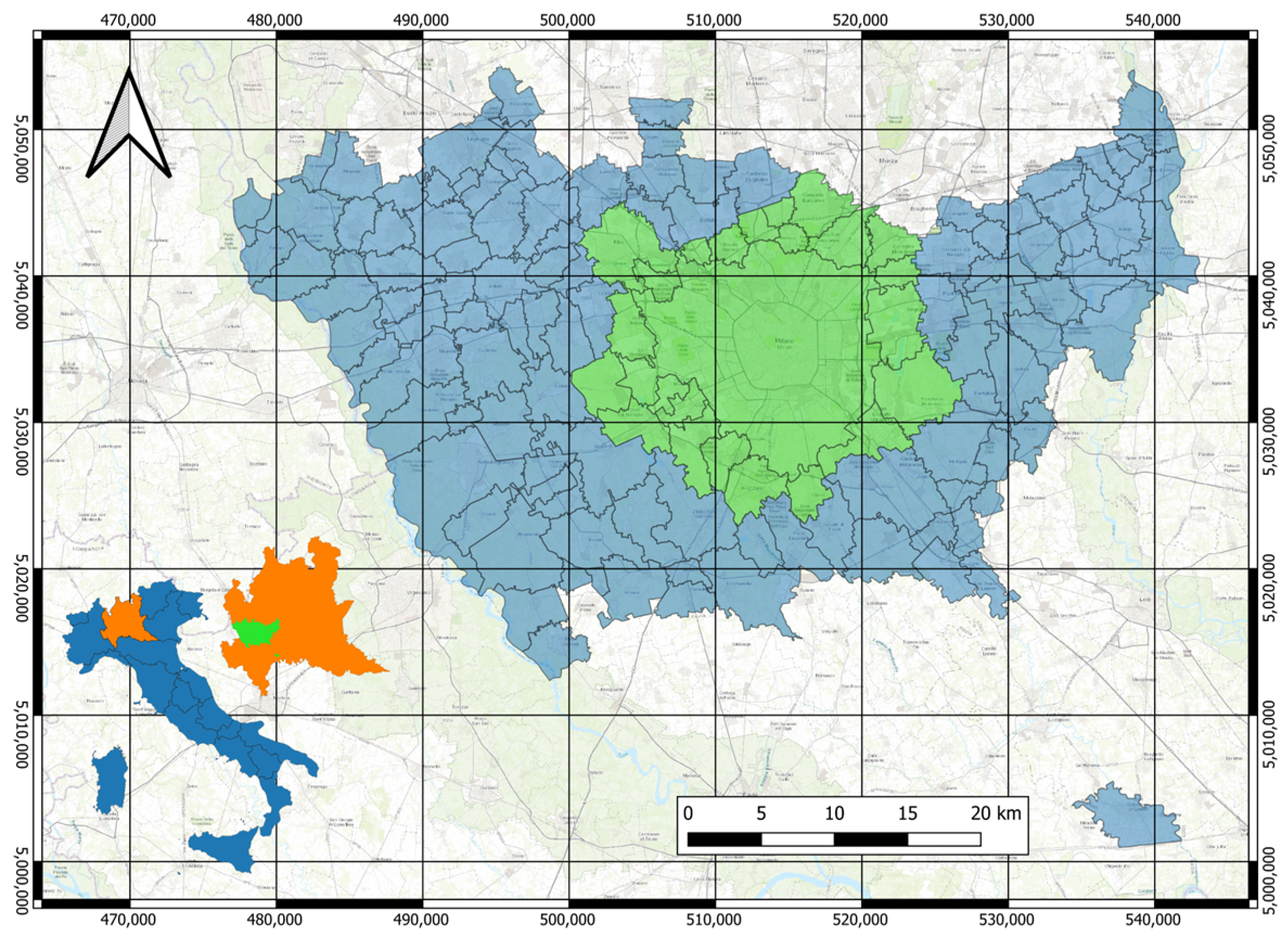
Milan, located in the Lombardy region, Northern Italy (Figure 1), has started a project to acquire a detailed digital twin of the metropolitan area. A call for tenders was published in late 2020 regarding acquiring aerial nadir and oblique images, LiDAR, and terrestrial mobile mapping data.
A temporary joint venture composed of four companies won the tender. CGR is an Italian company located in Parma, near the airport, which serves as the operating base for its fleet of aircraft. The company is a leading provider of photogrammetry and remote sensing services throughout Europe, incorporating advanced digital sensor technologies, including LiDARs and multispectral sensors. CycloMedia is a Dutch company that uses a specialized MMS (mobile mapping system) technology to acquire LiDAR, capture 360° panoramic photographs of large areas, and store them in an online database to visualize and manage environments systematically. ESRI Italia S.p.A. is a prominent member of ESRI One Company and serves as the official distributor of its products in Italy. The company specializes in geospatial solutions and provides comprehensive services and support for all application areas where geoinformation data are essential. SIT S.r.l. is an Italian company recently acquired by MERMEC Engineering and has experience in topographic and cartographic sectors, including surveying, geodata processing, cartography production, and geodatabase creation. Each company’s role in the venture is closely tied to their skills. CGR was responsible for surveying and processing all aerial data, while CycloMedia was tasked with mobile mapping surveying. ESRI Italia managed the produced data, and SIT created and measured the ground control network. Finally, the Laboratory of Geomatics at the University of Pavia, with over 40 years of experience in land and aerial surveying and geographical information, was assigned to analyze the quality of all acquired datasets.
The project started in 2022, and aims to gather aerial images that include nadiral and oblique perspectives, LiDAR points, and terrestrial mobile mapping data. The project features various conventional and groundbreaking products: true orthophotos (RGB and CIR), classified LiDAR point clouds, and DTM and DSM models derived from aerial surveying. In the meantime, terrestrial mobile mapping will offer point clouds, spherical depth images, and a database of 22 city objects, such as lighting poles, road markings, and driveways, to name a few. This database will host roughly 1.2 million elements identified, located, and characterized through artificial intelligence.
The metropolitan area has been split into two zones. Zona1 comprises the city of Milan and its neighboring municipalities, while Zona2 includes the remaining areas. Figure 1 illustrates the division, with Zona1 and Zona2 colored in green and blue, respectively. The larger polygon in the center represents the Municipality of Milan. The project encompasses 133 municipalities, including the San Colombano al Lambro exclave, which can be seen as the isolated polygon in the lower right corner of Figure 1.
The technical specifications for the tender outline the parameters for acquiring data according to different areas. The entire region must be captured with nadir imagery and LiDAR, with a resolution of 5 cm and a density of 20 points per square meter. Oblique images are only necessary for Zona1, while the MMS survey covers roads in the Municipality of Milano. However, it was decided that the same aerial data types for Zona1 and Zona2 would be acquired under the joint ventures, resulting in both areas having oblique and nadiral imagery. The aerial survey was conducted using Leica CityMapper-2, a hybrid system described in detail in the following section, and covered an area of 1776 square kilometers. The MMS survey was conducted using CycloMedia’s system, covering approximately 2555 km. To guarantee uniform quality and consistent geometry across all datasets, the project involves leveraging advanced GNSS and terrestrial LiDAR measurements. These tools will serve dual purposes: reliable ground control and thorough independent quality checks.
Furthermore, the requirements for the tender necessitate software tools to enable users to access complex datasets seamlessly. The project includes two main tools: a web application that promotes data sharing among all municipalities in the metropolitan area and a plugin for the ESRI ArcGIS™ (Redlands, CA, USA) environment. The latter is particularly valuable since the Municipality of Milan has adopted the platform as a standard tool for managing geographic information. The emphasis on software tools underscores the municipality’s recognition that having appropriate and user-friendly tools is crucial for capitalizing on the advanced and detailed datasets obtained.
All the surveys have been completed, and the final dataset is expected to be available within 2023. Some of the data, specifically the LiDAR data for Zona1, have already been provided for quality checks and will be the object of the present paper. However, the preliminary information has enabled an evaluation of the survey’s consistency, and the findings are outlined in Table 1. CGR collected all aerial datasets, including imagery and LiDAR data. To gather this information, they utilized the Leica CityMapper-2 sensor, known for its high accuracy and reliability. On the other hand, CycloMedia used its systems to acquire mobile mapping datasets consisting of images and point clouds [32].
1.2. The Leica CityMapper-2 Hybrid Sensor
The generation of digital twins requires the availability of multiple data, imagery, LiDAR, and aerial sensors capable of simultaneously collecting such types of information ideally suited for this task. In 2016, Leica Geosystems presented the first hybrid sensor called Leica CityMapper, and in 2021, they introduced the new CityMapper-2 [33]. The hybrid airborne sensor can capture both nadir and oblique imagery. It can take two nadir RGB/NIR images and four oblique RGB 150 MP images, providing a detailed view of the target area from multiple angles. Additionally, it can gather LiDAR data, allowing for precise measurements of elevation and terrain features. With this combination of technologies, the sensor provides a comprehensive and detailed understanding of the target area, making it an invaluable tool for various applications.
Focusing on LiDAR, the new system adopts a Leica Hyperion2+ unit with a pulse repetition rate of up to 2 MHz (against 700 kHz of the first version), the capability of handling up to 15 returns (with up to 35 multiple-pulse-in-the-air values), an operation altitude between 300 and 5500 m AGL (above ground level) and a theoretical vertical accuracy of <5 cm, at 1000 m AGL and with a 60 m/s aircraft speed.
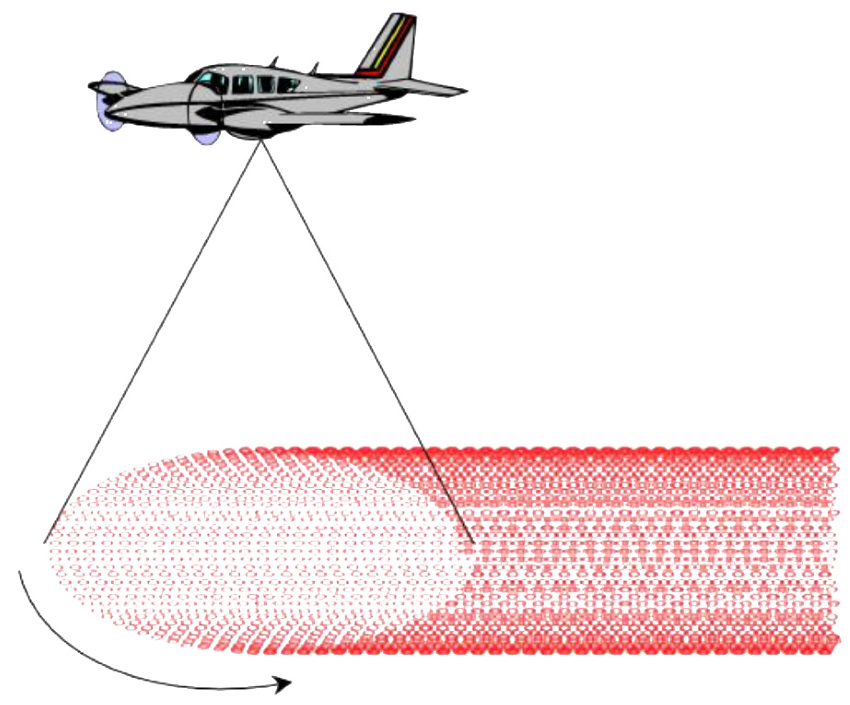
The Leica CityMapper-2 system implements a rotating scan wedge with a tilted rotational axis, the so-called Palmer scanner, characterized by oblique scanning with a constant laser beam off-nadir angle that produces a spiral-shaped scan pattern on the ground [19]. Oblique scanning allows one to look under overpasses or bridges, potentially providing more returns from facades, depending on building height, road width, and laser beam tilt. Moreover, it enables a backward and forward look along the same scan strip, thus allowing the surveying of objects from different viewpoints. However, this scanning mechanism causes an inhomogeneous point distribution with a much higher density on the border than that in the strip’s center (Figure 2); nevertheless, this could be useful for improving management between adjacent strips. This phenomenon has been investigated during data analysis, and the results are reported in Section 3.2.
2. Materials
Milano’s digital twin project is ongoing, and data processing is currently underway. Nevertheless, a significant portion of the LiDAR data related to the Municipality of Milan and the surrounding area (the so-called Zona1) are already available for quality evaluation. Moreover, preliminarily to aerial missions, complex GNSS and terrestrial LiDAR measurements were taken to guarantee good geometric consistency and uniform quality among data.
This section describes the main characteristics of the LiDAR data and the ground control network. Data processing was performed by CGR and MerMec Engineering, respectively, for LiDAR and topographic datasets. As the project tester, the Laboratory of Geomatics of the University of Pavia has performed the quality analysis. LiDAR data assessment, the subject of this paper, is exhaustively reported in Section 3, while the quality ground control network is briefly discussed in Section 2.2.
2.1. LiDAR Dataset
The paper concerns the LiDAR data that refer to Zona1. Flights were performed between the end of May and the beginning of June 2022, taking 6 days. The acquisitions comprised 87 east–west strips and 3 north–south ones; all strips were approximately 30 km long and were taken at 1500 m above ground level (AGL) with a field of view (FOV) of 36°.
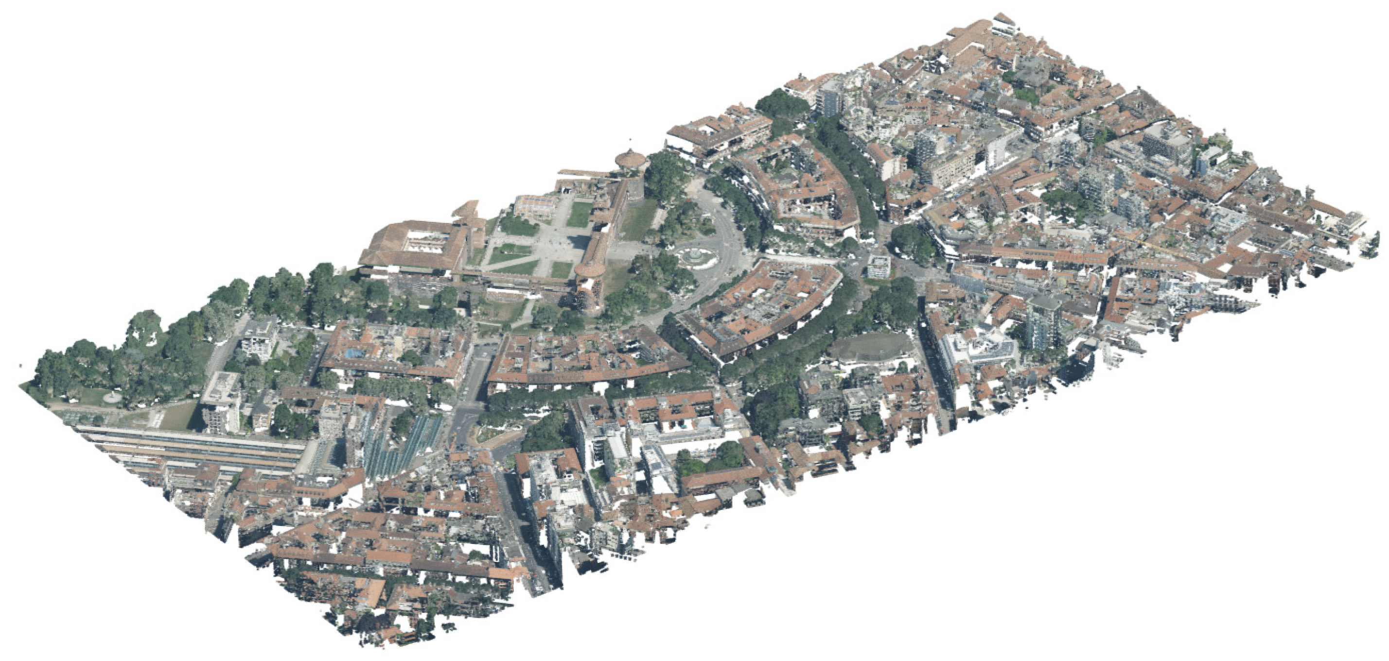
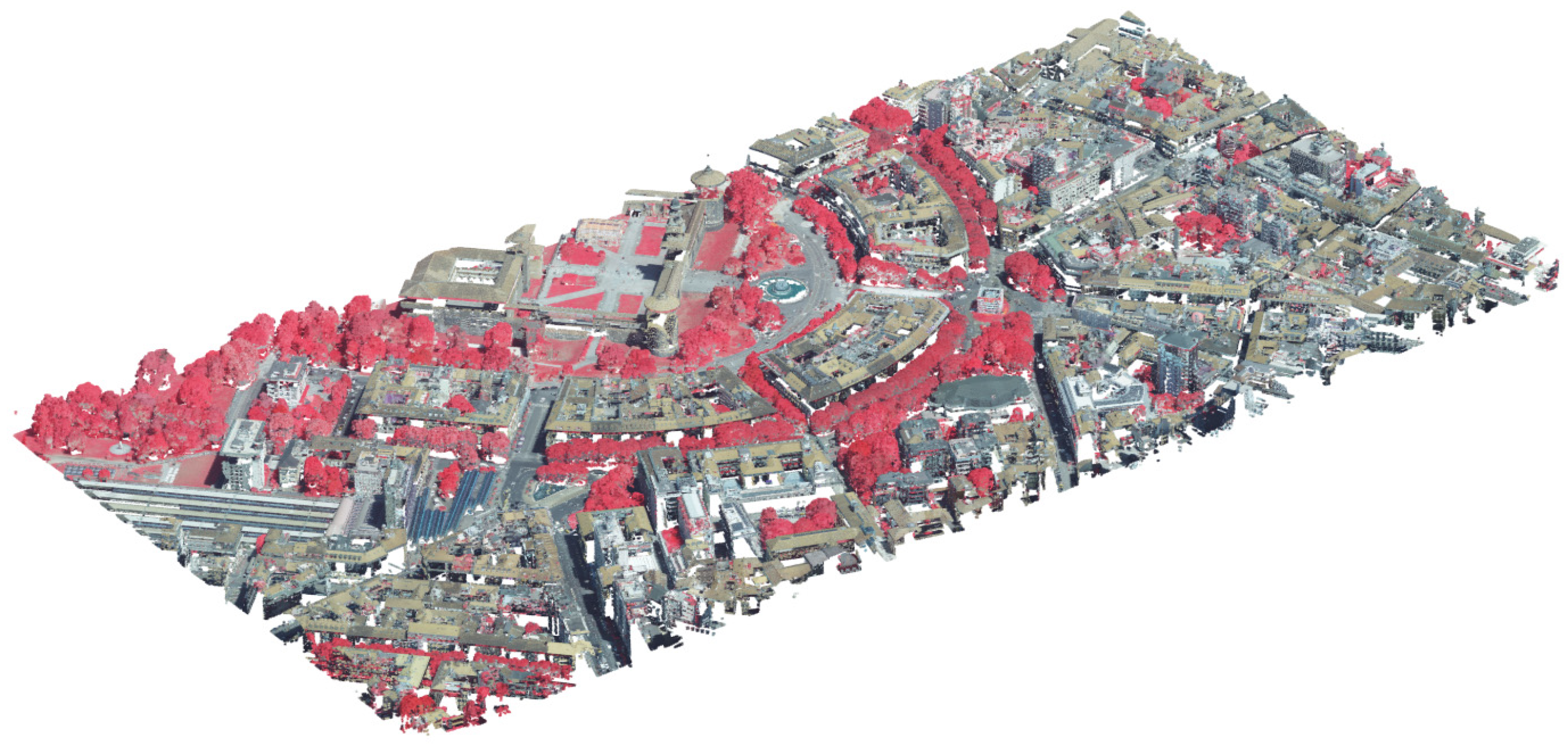
CGR has performed data processing with the Leica HxMap software package capable of accomplishing the whole LiDAR processing workflow: autocalibration, registration, color encoding, data metrics, and quality check (QC). Data were oriented via direct georeferencing in which the Piedmont–Lombardy GNSS permanent network was exploited for GNSS processing. The same geodetic infrastructure was also used for ground network adjustment, ensuring consistency between data. The software package also performs a double-vertical accuracy test analyzing the data congruency between flight lines and along the same scan direction. Two-meter side patches are extracted from LiDAR data, and vertical distances are calculated (the distance between the patches extracted in adjacent strips and patches extracted in the same strip considering forward and backward scan wedge orientations), classifying results according to the obtained values. Four categories are considered: less than 3 cm, between 3 and 5 cm, between 5 and 10 cm, and more than 10 cm. If cross-strip analysis can be considered quite usual, the accompanying scan direction assessment is atypical but necessary considering the presence of a double-wedge system. For system calibration and alignment, only patches with a standard deviation of less than 5 cm that are deemed reliable are considered; any patches with high residuals are disregarded. The outcomes of the assessment detailed in Section 3 demonstrate the effectiveness of this step. Point clouds were colored, exploiting a part of the Leica CityMapper2 imagery system, composed of a couple of nadir cameras capable of acquiring RGB and NIR bands. This characteristic allows the generation of point clouds with four color information and producing traditional RGB point clouds (Figure 3) or Color InfraRed one—CIR (Figure 4).
Finally, to facilitate data exchange between the temporary joint venture and the project tester, LiDAR data were subdivided into 1000 × 500 m2 tiles; altogether, Zona1 is composed of 2569 LAS files, containing 6 × 10¹⁰ points for an overall storage occupation of 2.08 TB.
2.2. Ground Control Network
One of the most qualifying elements of Milan’s digital twin project has been the creation of a ground control network useful for data processing under the temporary joint venture and for rigorous and independent quality checks by the project testers.
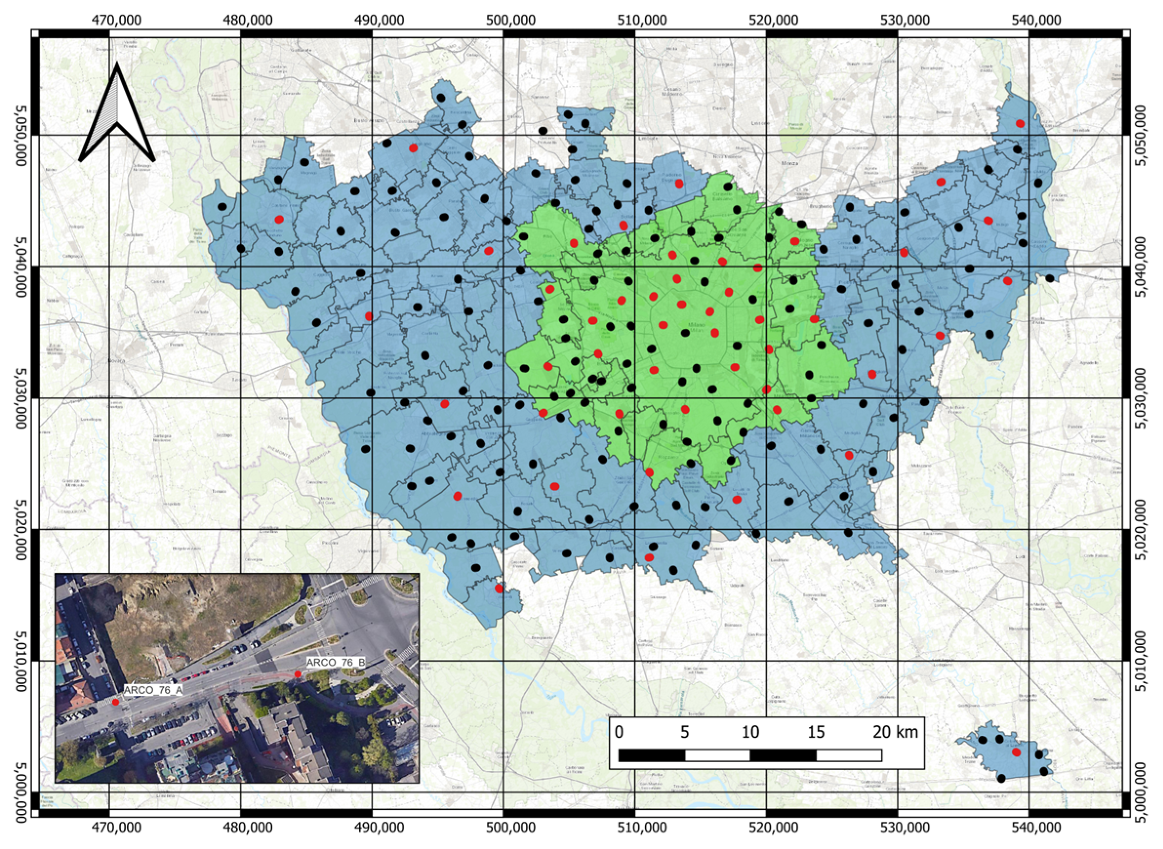
The network comprises 200 control areas, called ARCOs from the Italian “ARee di COntrollo”. Their distribution is reported in Figure 5; each ARCO comprises two benchmarks, at approximately 100 m apart:
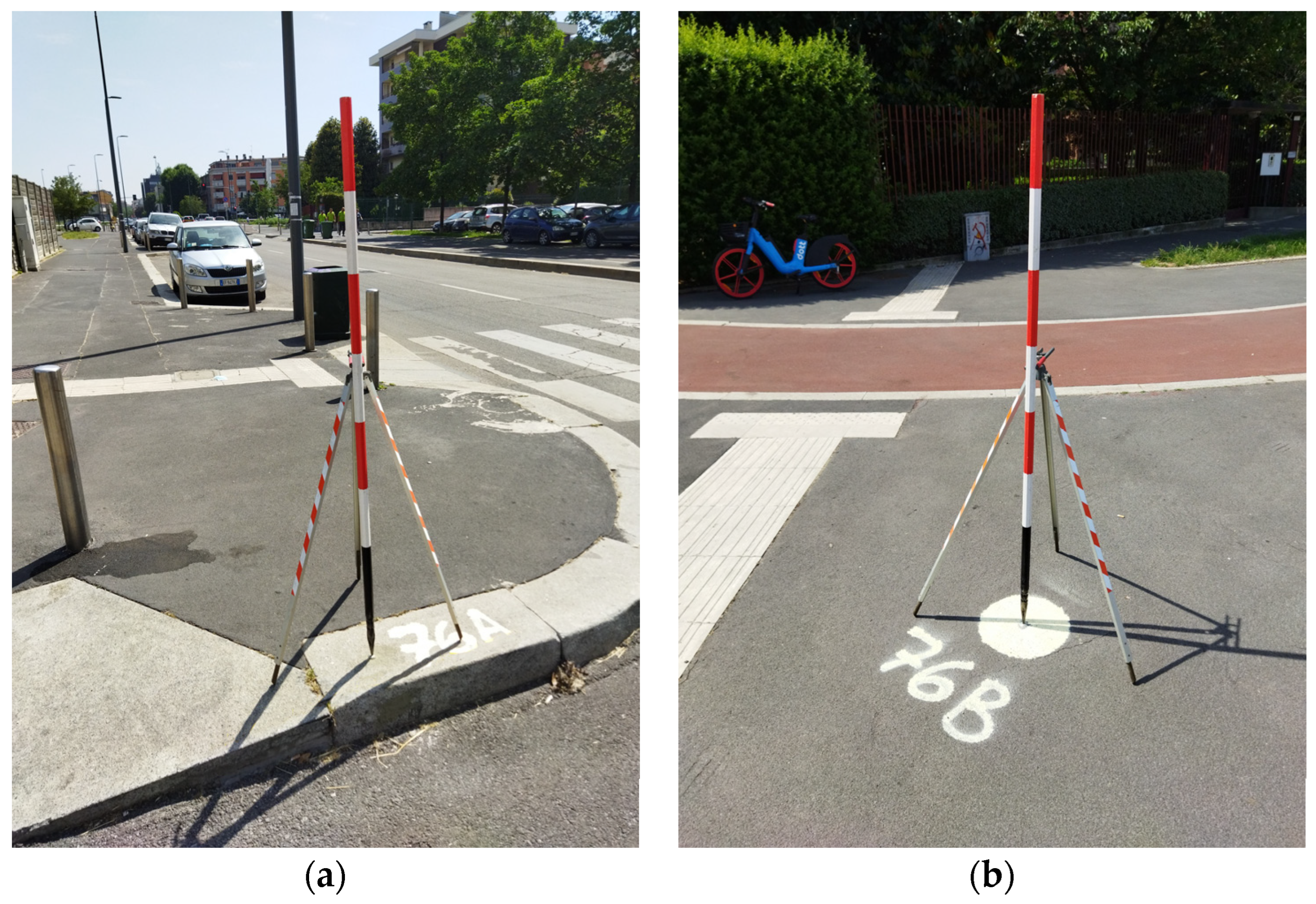
- A topographic nail stuck into a stable element (e.g., a concrete curb) and identified via the letter “A” (Figure 6a).
- A photogrammetric marker constituted by a white circle, with a radius of 15 cm, directly painted on the ground (asphalt, paver blocks, etc.), and identified via the letter “B” (Figure 6b). In the surroundings of each marker, with a minimum radius of 1 m and recommended of 2 m, the terrain can be comparable to a plane, not necessarily horizontal, without obstacles or slope variations (in case of a non-horizontal plane, its inclination is considered during the assessment, as better explained in Section 3.3.1). This characteristic makes the area around the markers useful for LiDAR vertical quality assessment and density estimation.
The benchmarks were surveyed with a redundant static GNSS network, employing multi-frequency and multi-constellation receivers. Since the aerial imagery has a ground sampling distance (GSD) of 5 cm, using a static network is mandatory to guarantee sufficient accuracy in the ground truth. Table 2 reports the mean, the root mean square (RMS), and the RMSE obtained for the three components and the two typologies of vertices. The RMSE was determined using the formulas specified by the U.S. Geological Survey (USGS) lidar base specification [34]. The statistics are separated for the two types of points since they were measured differently: ARCOs-typeA were connected within a network, reaching a relative redundancy between 3 and 5; ARCOs-typeB were only connected with the two typesA’s points more closely, reaching a redundancy of 2. This explains why the latter performs a bit worse than the former does. The technical specifications for the tender require a maximum RMSE value of 15 mm for the horizontal components and 22 mm for the vertical component. The network compensation meets both requirements. Nevertheless, all the components show non-zero values for the mean; this could be due to the use of a simplified antenna model for some SPIN3 stations during network adjustment.
For LiDAR data analysis purposes, 50 of 200 ARCOs were also surveyed using a terrestrial laser scanner (TLS). The selection of these so-called Special-ARCOs was based mainly on the presence of elements useful for assessing horizontal and vertical point cloud accuracy. Indeed, the selected areas had to be characterized by the following:
- The presence of one or more manmade elements (e.g., buildings, garages, or bus shelters) with at least two vertical perpendicular sides;
- The presence of any flat areas located at a different height to street level;
- The presence of large road markings (e.g., zebra crossing) of a good preservation state.
Figure 5.
Location of the 200 ARCOs; red dots represent the Special-ARCOs (polygons color have the same meaning as Figure 1). The small frame shows an example of the relative position of the two ARCO benchmarks (the example reports the same ARCO shown in Figure 6).

Figure 6.
An example of ARCOs: (a) TypeA benchmark stuck in a large concrete curb; (b) TypeB photogrammetric marker positioned in a flat area, without obstacles or slope variations in a neighborhood of 2 m.
Figure 6.
An example of ARCOs: (a) TypeA benchmark stuck in a large concrete curb; (b) TypeB photogrammetric marker positioned in a flat area, without obstacles or slope variations in a neighborhood of 2 m.

Figure 5 shows, with red dots, the positions of the Special-ARCOs. Altogether, considering the only Zona1 area where LiDAR data are currently available, there are 76 ARCOs, of which 33 are Special-ARCOs. The analysis reported in Section 3 refers to these data.
The Special-ARCOs were surveyed with the Riegl VZ®-400i terrestrial laser scanner equipped with a reflex camera for producing colored point clouds. Each ARCO was scanned from a single station, taking care to orient the instrument according to typeA and typeB benchmarks. The scan rate was set to 300 kHz, and the acquisitions were settled to guarantee a spatial resolution of less than or equal to 3 cm at 100 m distance.
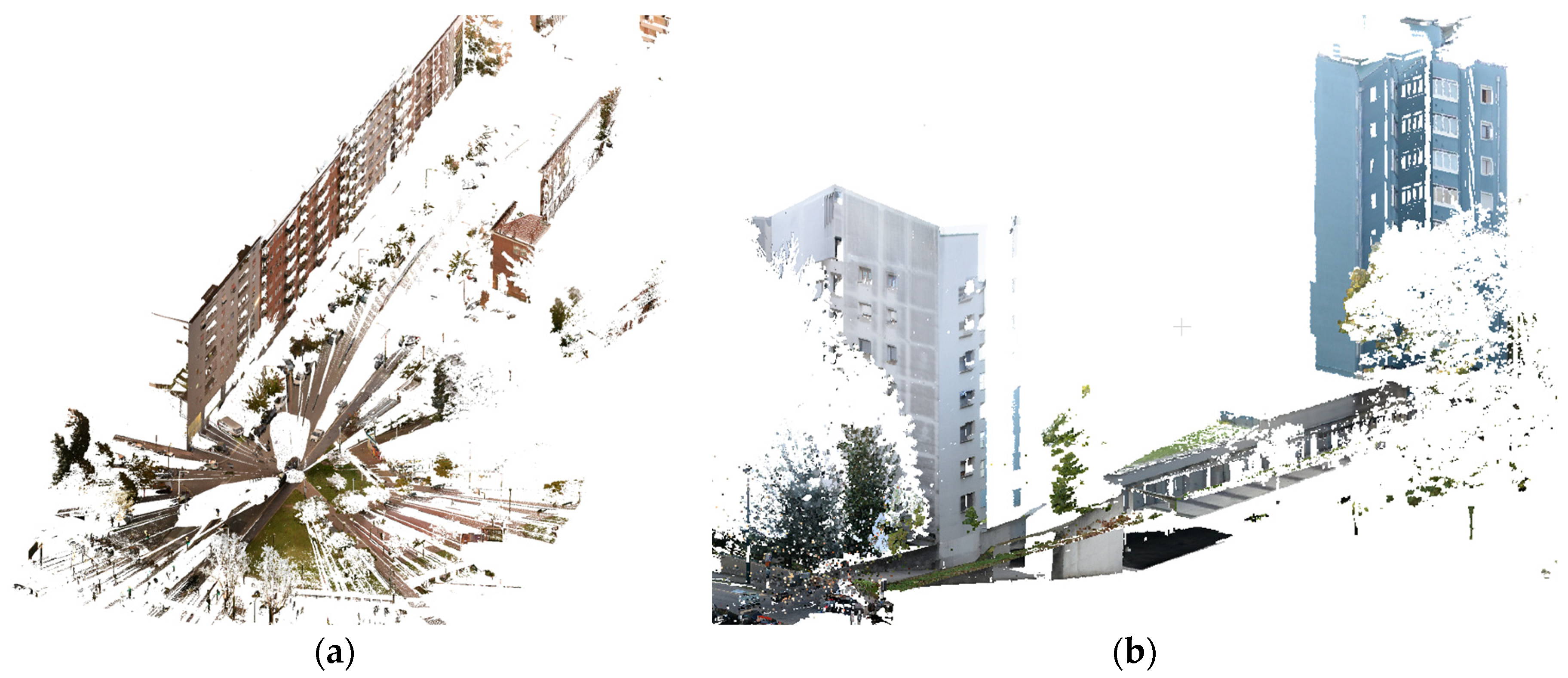
Figure 7 reports some examples of Special-ARCOs: both images show buildings in which it is possible to identify two vertical and perpendicular surfaces, at least 2 m2 wide, constituted by the facades. As explained in Section 3, this information can be used to quantify possible horizontal biases between LiDAR data and TLS acquisition.
Six out of fifty Special-ARCOs, corresponding to approximately 10%, were also independently surveyed by the project testers for quality checks. A Leica MS60 ScanStation was employed; the instrument is a traditional total station capable of performing scans. As the two TLS clouds, obtained by the company and the testers, are perfectly co-registered thanks to the use of the same benchmark coordinates for the orientation, the scans were compared through a cloud-to-cloud approach. The overall RMS is about 1.3 cm, showing that the control data have characteristics suitable for the following aerial LiDAR quality analysis.
3. Assessment of the Leica CityMapper-2 LiDAR Data
The Municipality of Milan has placed great expectations on the digital twin project’s repercussions on the city in many ways (e.g., management, sustainability, economy, etc.). As reported in the introductory section, many data sources were acquired: aerial imagery, aerial LiDAR, and mobile mapping system data. Congruency between all these data and their 3D accuracy and precision are mandatory. As reported in Section 2.2, a complex ground control network has been created to guarantee these aspects, and several procedures have been foreseen to assess these parameters. The tests were conducted in the MATLAB R2022b environment, in which dedicated codes were prepared to manage, visualize, and analyze all the available data. All the analyses are conducted fully automatically, with the only exception being the use of large road markings in which human visual comparison is performed. Finally, the analysis concerns the overlap between adjacent strips, the point cloud density, and LiDAR quality analysis for both vertical and horizontal components.
3.1. Quantification of the Overlap between Adjacent Strips
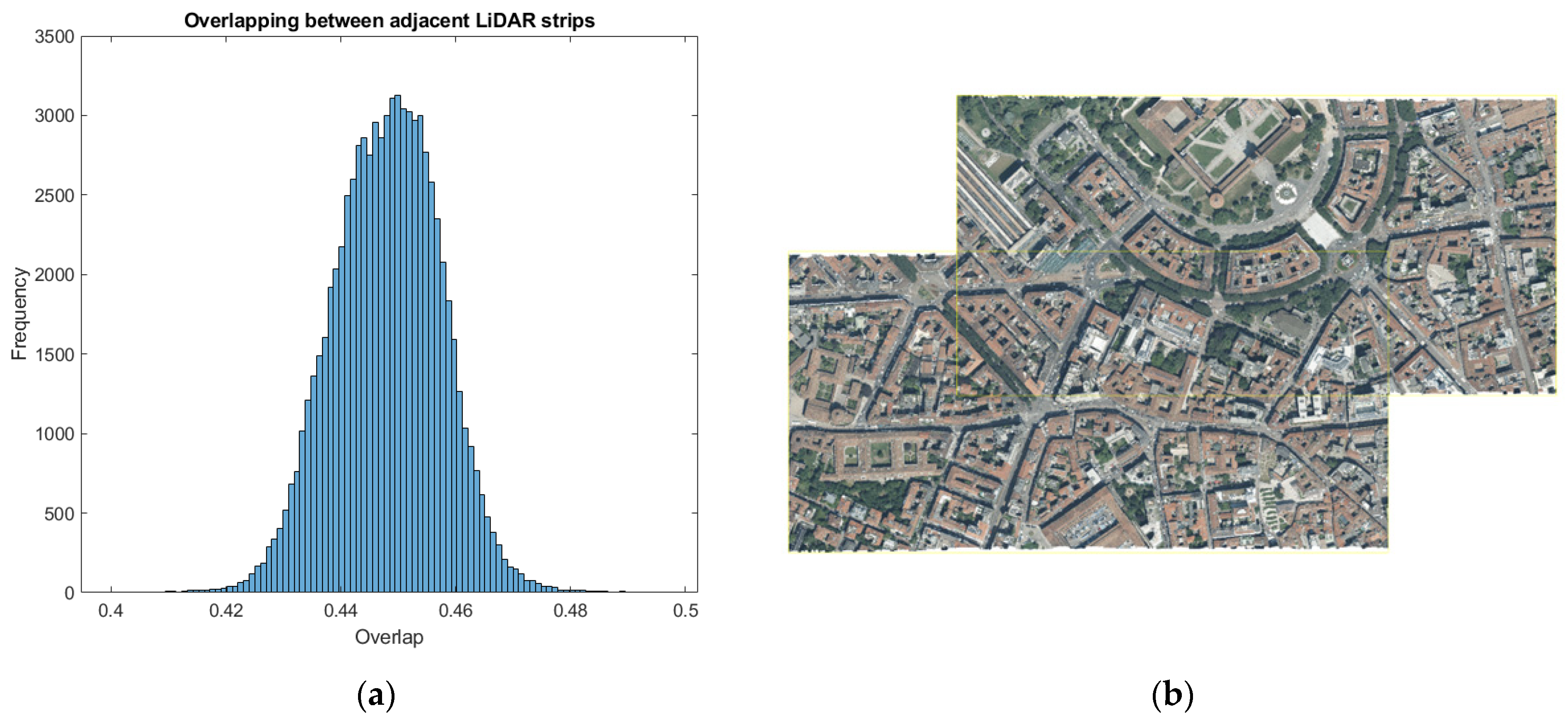
The technical specification of the call for tenders provides a minimum overlap between adjacent strips of 10%. However, the use of a hybrid system has meant that photogrammetric planning prevails over LiDAR planning; since photogrammetry requires large overlapping, at greater than 10%, this requisite could be considered automatically guaranteed. However, the overlap has been systematically calculated from the knowledge of the sensor exterior orientations, the field of view (FOV), and the digital terrain model (DTM).
3.2. Point Cloud Density Estimation
Point cloud density and its variations inside blocks impact derived products, such as DSM or DTM, and must be evaluated [35]. In this work, it is evaluated considering each strip individually and taking into consideration the whole dataset. This double estimation allows us to analyze the influence and the interaction between the acquisition method (the circular oblique scanning pattern) and the high overlap.
Density is quantified thanks to the flat terrain surrounding ARCOs-typeB; in particular, for each of them, a four-square-meter area is considered, the inside points are counted, and the relative density is determined. The technical specification of the call for tenders provides a minimum density of 20 pts/m2. As LiDAR data are only available for Area1, density was computed using only 76 of the 200 ARCOs.
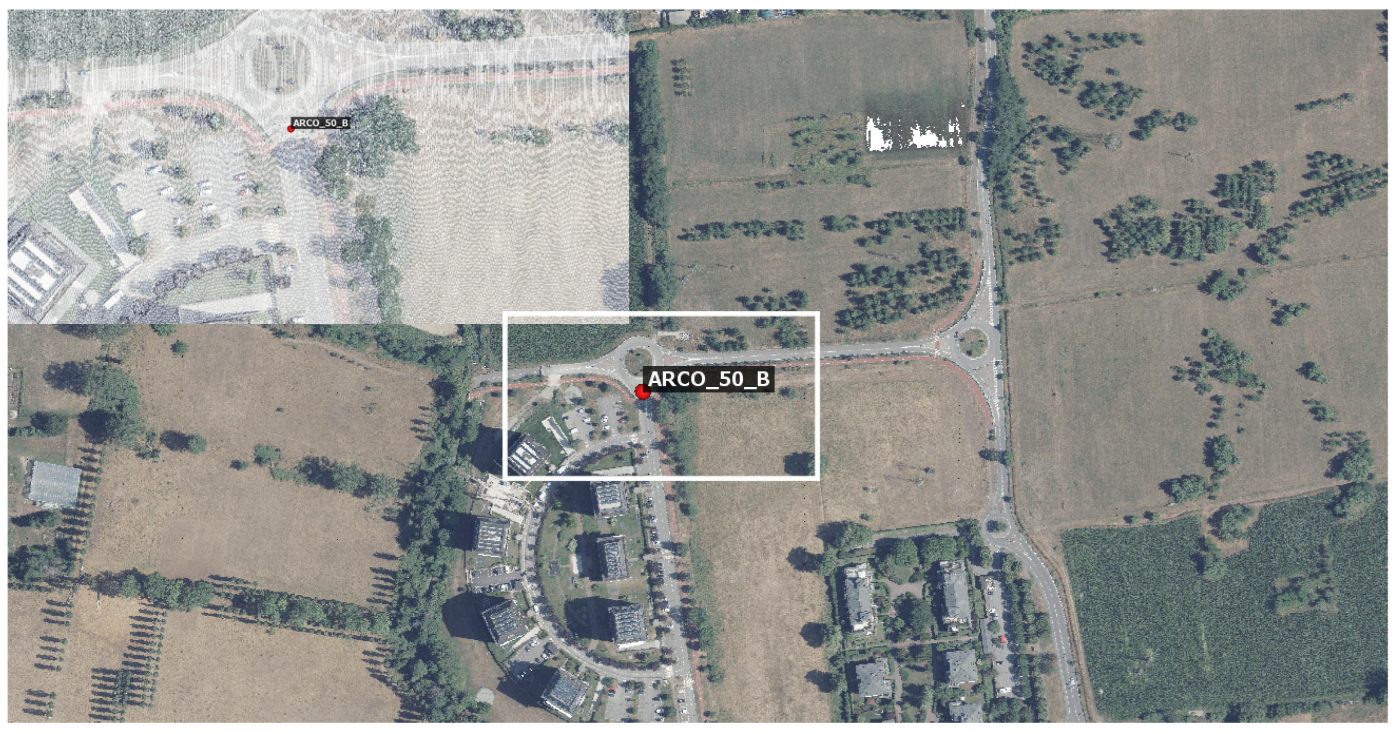
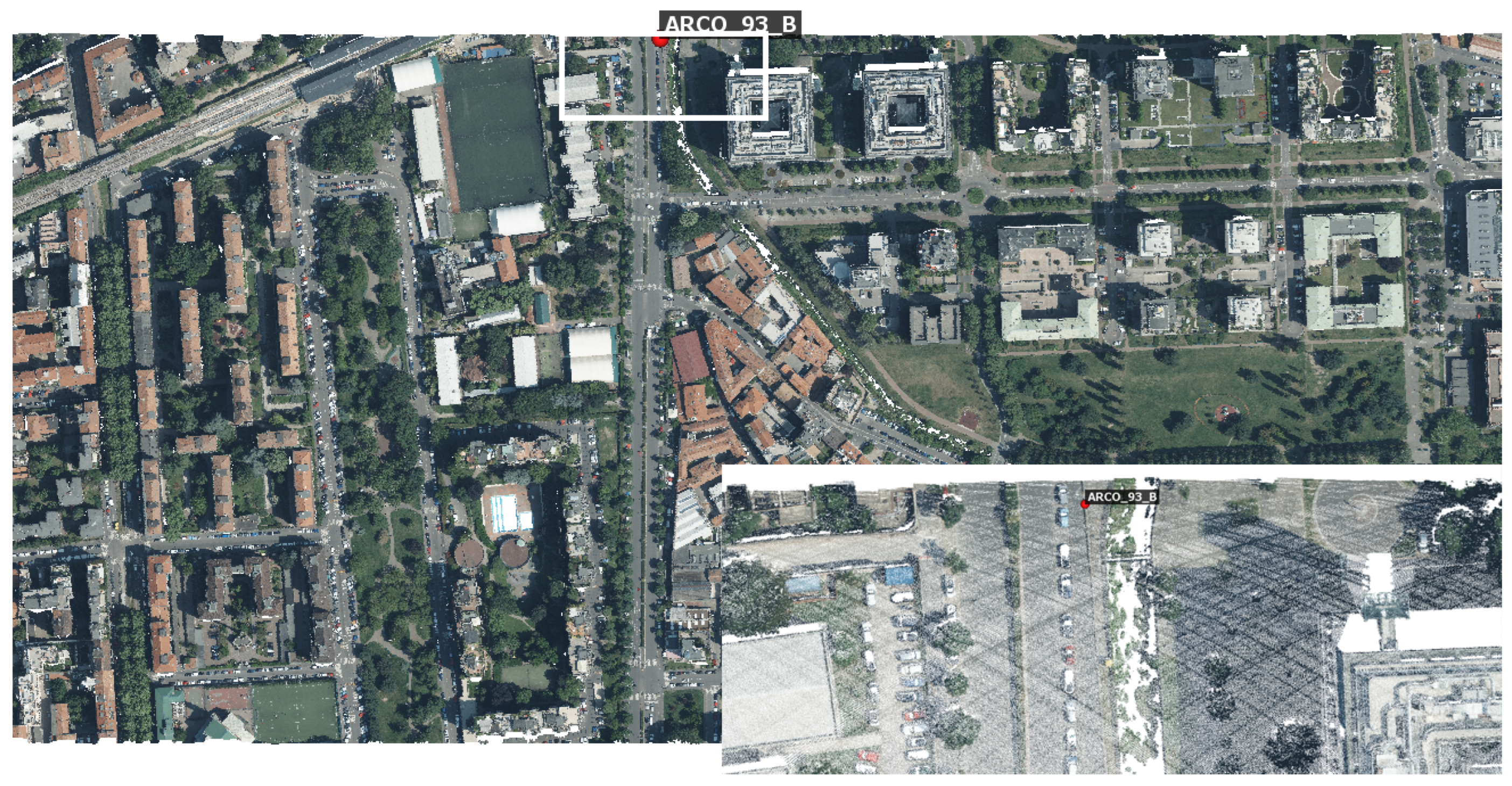
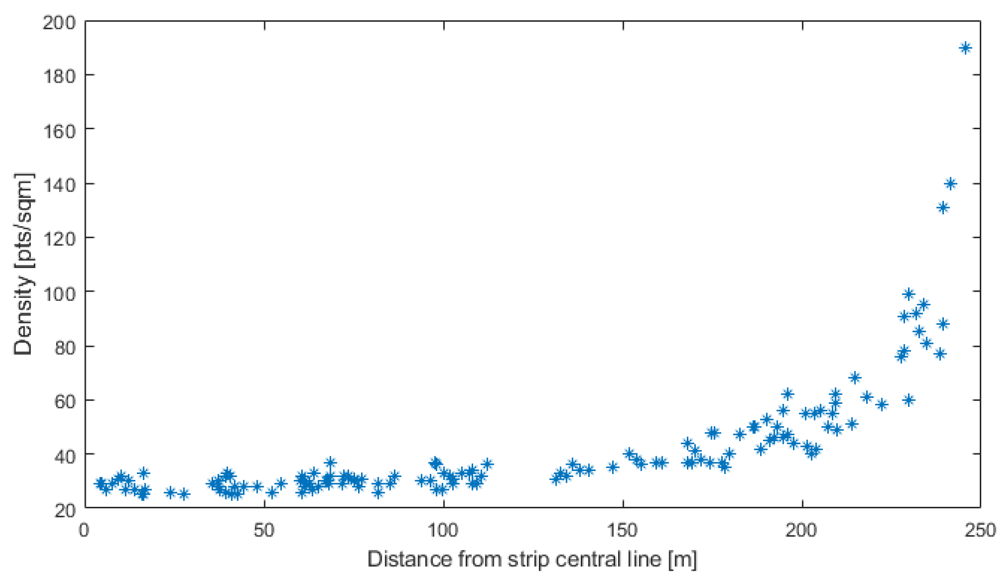
Considering all the strips separately, density ranges between 25 pts/m2 and 190 pts/m2 for ARCO_50B and ARCO_93B, respectively; the median value is 33 pts/m2. Figure 9 shows ARCO_50B located substantially near the strip’s central line where the scanning pattern is weaker; on the other hand, Figure 10 shows the location of ARCO_93B, which falls near the strip’s border where points are denser. The analysis of individual strips shows how the threshold for density is always respected; still, the circular acquisition pattern causes significant inhomogeneity moving from the center to the strip’s edges. This phenomenon is visible in the plotting of the point density for the tested ARCOs according to their distance from the strip’s central line, as shown in Figure 11; the density increases slowly until it reaches 80% of the half-width of the strip and then grows exponentially.
A hybrid system, such as the Leica CityMapper-2, produces a high level of overlap between strips since photogrammetric planning prevails over LiDAR planning. This condition appreciably changes the point cloud density when the acquired data are considered. Repeating the above-illustrated analysis for the complete dataset, the median passes from 33 pts/m2 to 77 pts/m2. Nevertheless, this higher density can be properly exploited only if the strips are consistent; this aspect will be analyzed in the next sections.
3.3. LiDAR Point Clouds Quality Analysis
When evaluating LiDAR data, three attributes are considered [34,36]: accuracy, precision, and congruency between adjacent strips. The terms accuracy and precision are used in their most widespread meaning: accuracy refers to how close a measurement is to the true value; in contrast, precision refers to how close measurements are to each other. Assessing the congruency between adjacent strips is important, too.
Milan’s project involves two types of benchmarks that are useful for analysis: the flat terrain surrounding each ARCO-typeB marker and the Special-ARCOs (refer to Section 2.2 for more information). The flat terrain is only beneficial for vertical assessment, whereas the Special-ARCOs have beneficial properties for both vertical and horizontal components. Both benchmarks are utilized for accuracy and precision evaluations, and each strip is assessed separately. Congruency is evaluated using only the ARCOs-typeB and the high level of overlap available in Milan’s data.
The following sections present the assessment results divided in accordance with the ground network elements used for analyzing data quality: the ARCO-typeB marker and Special-ARCOs.
3.3.1. Assessments with ARCOs-typeB Vertices
As reported in Section 2.2, around each ARCO-typeB marker, within a radius of about 2 m, the terrain can be comparable to a flat surface (Figure 6b). All the LiDAR points, falling within a 4 m2 area around each benchmark, are extracted, and a robust plane is fitted on them. This approach has been followed because, even if the terrain is flat, it could not be rigorously horizontal, and the plane’s estimation allows us to consider any slope.
For fitting purposes, the M-estimator sample consensus (MSAC) algorithm, proposed by [37] as a variant of RANSAC, is used. Once the threshold for outliers’ identification is set, the algorithm estimates the parameters for the geometric model of the plane, the indices corresponding to inlier and outlier points, and the mean error of the distance of inlier points from the model. The outlier’s threshold is set to 18 cm, which is three times the maximum mean square error specified in the call for tender documents. Once the plane is determined, it is translated until the typeB marker lays on it; perpendicular distances between each inlier point belonging to the LiDAR cloud and the shifted plane are computed.
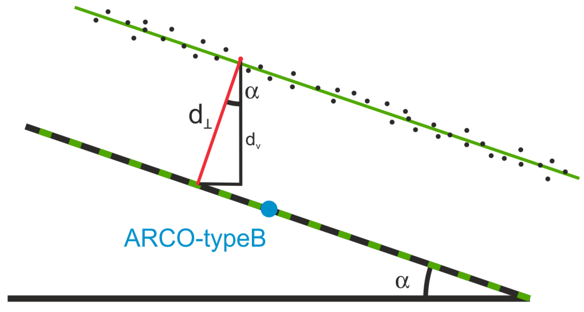
Figure 12 shows the procedure, in which black dots represent LiDAR measurements, while the green line is the robust plane fitted. The plane is translated until the typeB benchmark lays on it (black and green dashed line), and the vertical distances, d↖, between each LiDAR point and shifted plane are calculated. For readability reasons, for example, only one distance is drawn. If the area around the benchmark is horizontal, the calculated distance, the red line, represents the vertical error directly; otherwise, in the case of a sloped terrain, the vertical distance must be obtained considering this inclination in accordance with Formula (1):
in which the two distances, d↖ and dV, have the meaning shown in Figure 12 and a↦ is the plane inclination, obtainable from plane parameters. This is a well-known problem already faced by several authors [31,38]). As in our case, all of them decomposed the LiDAR data error in its components in accordance with the terrain’s slope.
dV = d↖ · cos (a↦),
Inclination angles of fitted planes are then systematically calculated and applied to the perpendicular distance. Considering all the strips separately, 139 ARCOs-typeB are analyzed for a total number of points of about 30k (only 42 outliers are detected, corresponding to less than 1%). Table 3 presents a numerical summary of the vertical accuracy assessment results, while Figure 13 visually represents the same results. The table includes five figures: the mean, RMS, RMSE, 95th percentile, and maximum value. Per the tender document’s specifications, only the reference values for the last two figures are reported in column two since a threshold is imposed on them.
For clarity, formulas for the mean, RMS, and RMSE are reported as the following:
When dealing with equations, the variable di refers to the distance between each aerial Li-DAR point and the fitted plane. It is important to note that the distance should be zero in an ideal world. However, in reality, several factors, such as atmospheric conditions, sensor and system calibration, and processing algorithms, prevent this from being the case. Furthermore, the ground control network influences this aspect, which is why Table 2 reports the GNSS static network quality. When analyzing a data set, the mean and root mean square (RMS) values are commonly used to determine the presence and nature of errors. If the mean value significantly differs from zero, systematic errors or biases may exist in the data. On the other hand, the RMS value can be used to estimate the magnitude of accidental errors. Finally, RMSE is a synthetic metric that comprehensively evaluates systematic and accidental error sources by measuring the dispersion of observations around zero. This metric is particularly useful when it is important to understand the level of accuracy or precision in a given dataset. By incorporating both types of errors into a single metric, RMSE offers a valuable tool for researchers and professionals seeking to assess the quality of measurements.
The estimated planes are used to evaluate the mean square error (MSE) of the LiDAR point clouds, as the MSAC algorithm also estimates the mean error of the distance of inlier points from the model. The technical specification of the call for tenders requires this value to be less than 6 cm. All the MSEs obtained via each plane estimation is well below this threshold; the overall mean is 1.1 cm, the RMS is 0.9 cm, and the RMSE is 1.4 cm.
Using LiDAR data requires that adjacent strips be consistent, and this aspect can be evaluated using the planes fitted on the point clouds around each ARCO-typeB. Since the high level of strip overlapping ensures that some markers are visible in two strips, the distance between their planes can be used to estimate their congruency. Rigorously, the two planes could be tilted toward each other, but considering the small sizes of the tested areas, measuring 4 m2, this issue can be neglected. Of the 76 ARCOs-typeB, 63 are present on two strips, so distances between related planes are calculated; the mean of distances between adjacent strips is 1.2 cm while the RMS is 1.2 cm, and the RMSE is 1.7 cm.
3.3.2. Assessments with Special-ARCOs
As explained in Section 2.2, Special-ARCOs are control areas surveyed with TLS to evaluate LiDAR data quality. Of the 50 Special-ARCOs, 24 fall into Zona1; points belonging to flat surfaces with a significant extension and density have been considered in each. Surfaces are both vertical and horizontal to evaluate both error components.
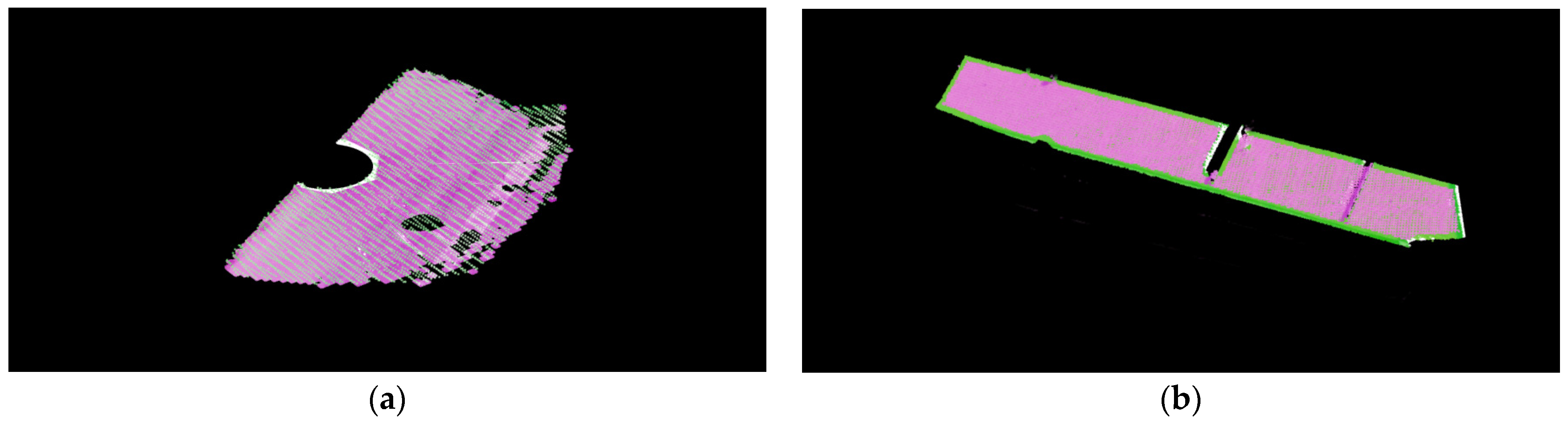
Concerning the vertical error, flat surfaces belonging mainly to roads and rooftops have been considered. These areas are extracted from the TLS datasets semi-automatically, tuning the selection parameters, such as extension, density, or planarity, in accordance with ARCO’s characteristics. Once identified in the terrestrial point cloud, the same area is trimmed on the aerial one. Figure 14 shows a couple of examples of this data: Figure 14a regards a portion of a road close to the TLS scan location, while Figure 14b reports an example on a rooftop. ALS and TLS data are reported in green and magenta, respectively.
The procedure for vertical assessment is like that illustrated in the previous section: for each Special-ARCO, a robust plane is fitted to the selected TLS data, and the perpendicular distances between each point belonging to the LiDAR cloud and the plane are computed. It is crucial to note that using a fitted plane to calculate the distance between two datasets is essential. When estimating mutual distances between two point clouds, the difference in density can affect the outcome. This issue has been studied extensively in terrestrial surveys [39], and various methods can be used, such as measurements of point-to-point distance, point-to-global surface, or point-to-local surface (the mutual distance metric used in this paper). A robust fitted plane, like the one utilized in this paper, can provide accurate results even when the density of the point clouds is significantly different.
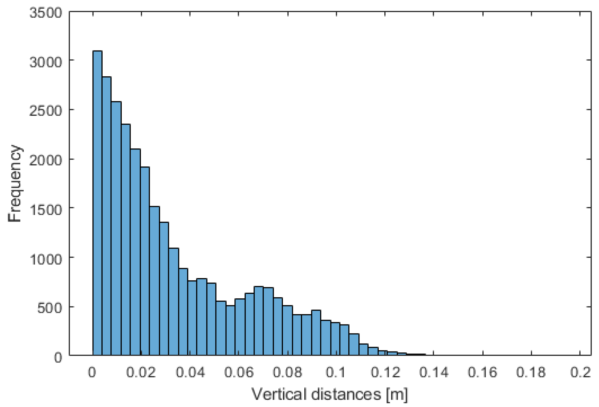
Pure vertical errors are then determined considering the plane slope and using Equation (1). Table 4 summarizes the obtained results, while Figure 15 shows them graphically through a histogram.
Concerning the LiDAR point clouds precisions, for Special-ARCOs, all MSEs obtained for each plane fitting are well below the threshold of 6 cm; the overall mean is 2.1 cm, the RMS is 1.4 cm, and the RMSE is 2.5 cm.
In Milan’s project, the inclination of the two Leica CityMapper2 wedges guarantees the surveying of points on the building facades, and this characteristic has been exploited to evaluate horizontal errors. The analysis is performed exploiting the Special-ARCOs since, in each of them, some vertical surfaces of buildings or similar structures were surveyed with a TLS system.
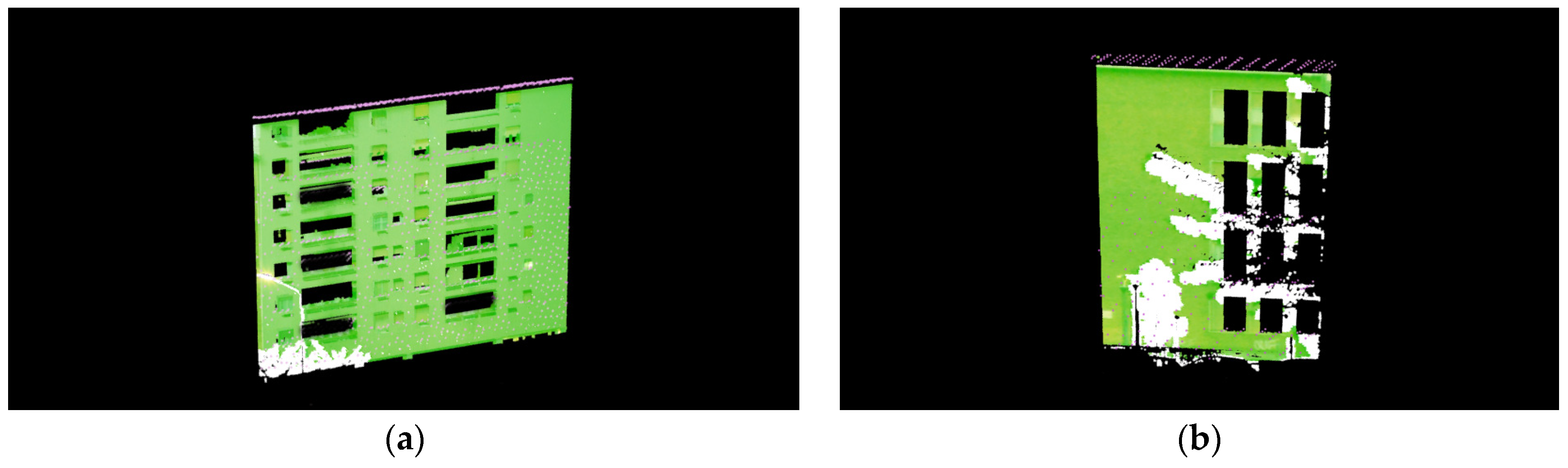
The evaluation of the horizontal errors is quite similar to that illustrated previously for vertical components, except that for manmade elements (e.g., buildings, garages, or bus shelters), vertical sides are considered. These areas are extracted from the TLS datasets in a semi-automatic way, tuning the selection parameters as the extension (at least 2 m2 wide), density, or planarity, according to the ARCO’s characteristics; for each check area, at least two vertical sides with a perpendicular orientation are considered. Once identified in the terrestrial point cloud, the same area is trimmed on the aerial one. Further bundler detection is performed to exclude from computation the points not belonging to the façade, such as windows, balconies, etc. Figure 16 shows, as an example, the data extracted for Special-ARCO 7, which are also shown in Figure 7a; ALS and TLS data are reported in green and magenta, respectively.
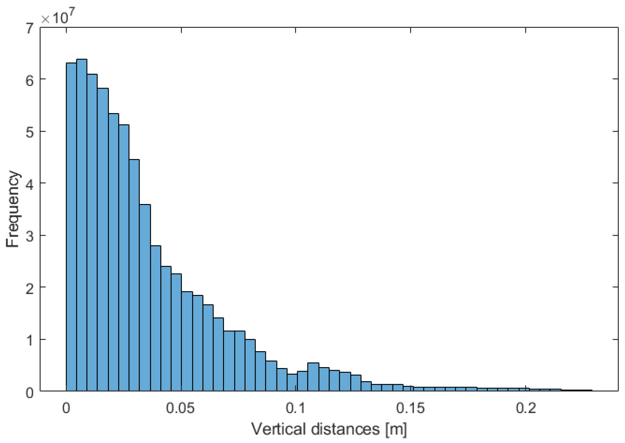
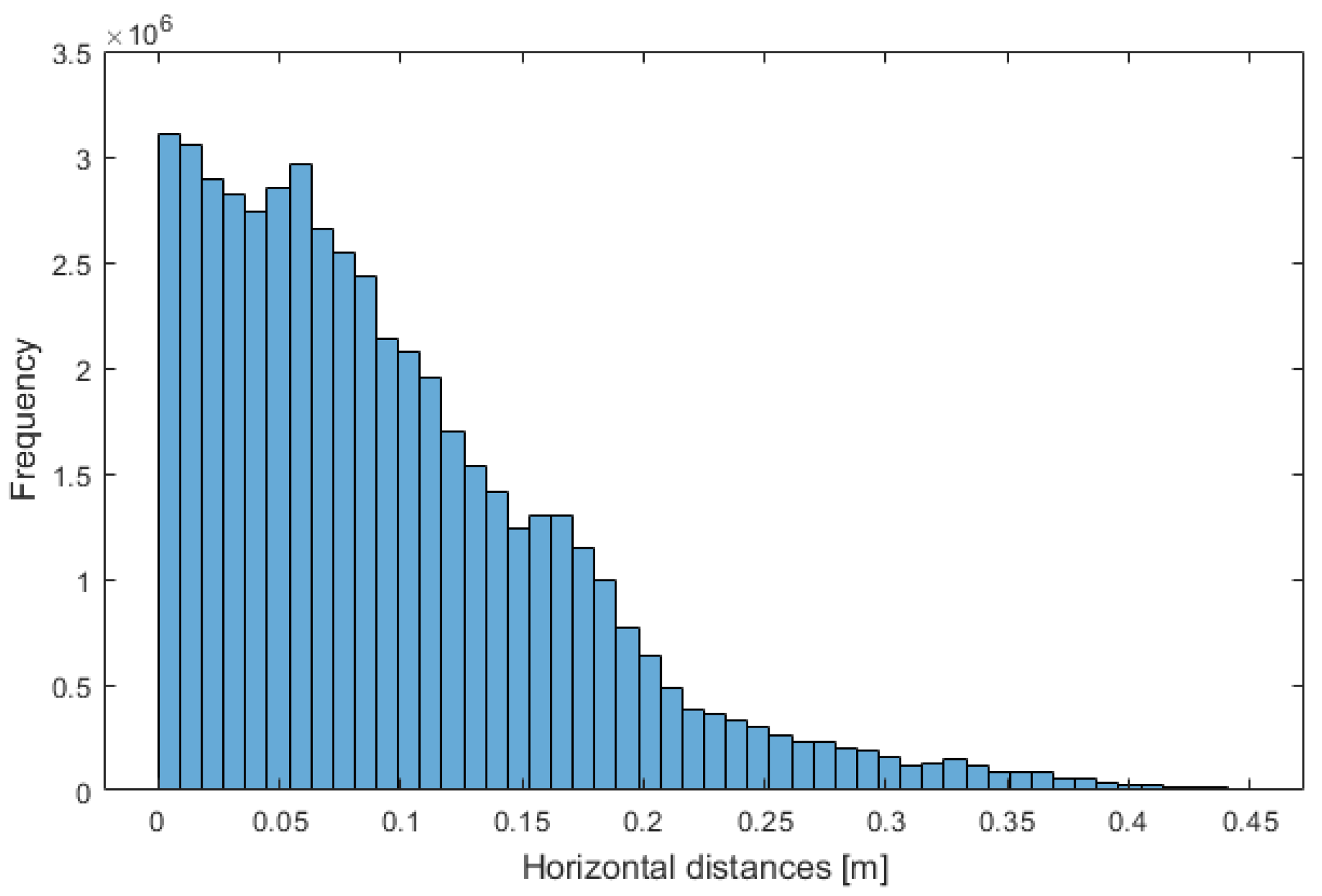
In each Special-ARCO, a robust plane is fitted to the selected TLS data, and the perpendicular distances between each point belonging to the aerial LiDAR cloud and the plane are computed. In this case, the estimated distance can be considered perfectly horizontal since only facades are considered; since two perpendicular surfaces are considered, the composition of their results allows us to estimate 2D horizontal errors. Table 5 summarizes the obtained results, while Figure 17 shows them graphically using a histogram.
Concerning the LiDAR point clouds’ horizontal precisions, all MSEs obtained via each round of plane fitting is well below the threshold of 18.4 cm; the overall mean is 8.5 cm, the RMS is 1.9 cm, and the RMSE is 8.7 cm.
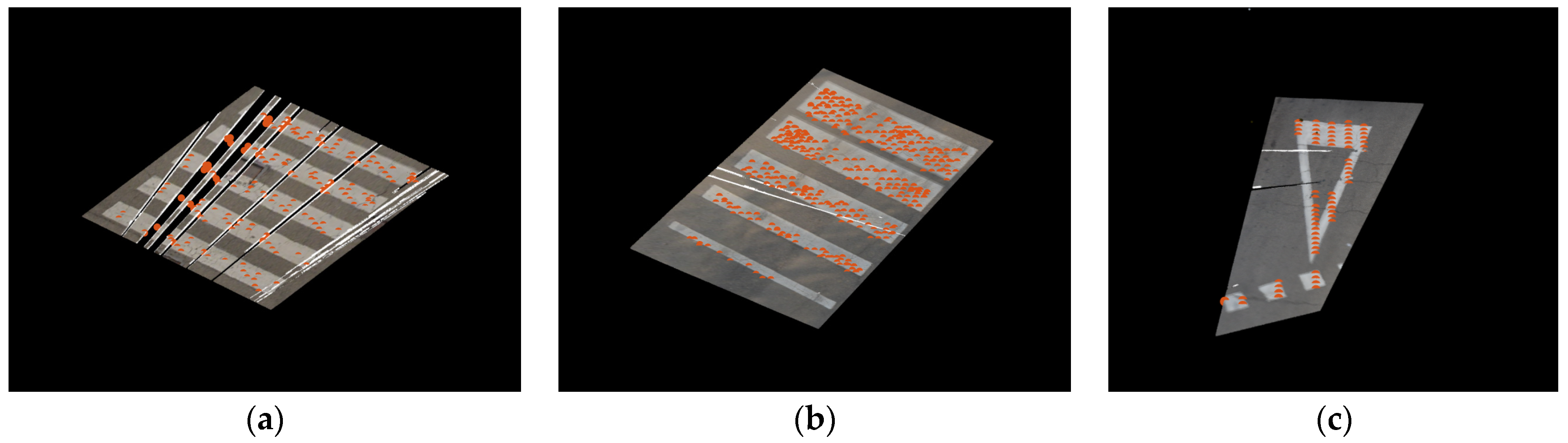
Finally, acquiring color and reflectivity information from both laser systems, terrestrial and aerial, allows us to evaluate the planimetric quality of georeferencing using road markings. For Special-ARCOs in which this type of element is present, areas containing road markings are extracted from the TLS datasets in a semi-automatic way, tuning the selection parameters, such as planimetry, terrain height, and the presence of high reflectivity points; once identified in the terrestrial point cloud, the same area is trimmed on the aerial one. Furthermore, for ALS data, only the points with high reflectivity are considered; the threshold is tuned according to each ARCO characteristic (paint degradation, the presence of a shadow, etc.). The clouds are plotted together, and a visual comparison is performed; in this case, no numerical values are extracted, but only an in–out evaluation is conducted. Figure 18 reports some examples of this analysis: the images show the extracted TLS datasets, colored in accordance with their RGB information, and the ALS-selected high-reflectivity points (orange dots); the size of these points is increased for the best readability. All the tested areas show good correspondence between the two data sets, passing the visual inspection.
4. Discussion
Full 3D accuracy and congruency assessments f LiDAR data have to become a standard practice in all data acquisition endeavors, especially in large-scale projects. LiDAR data standard specification documents are often very specific about the required horizontal and vertical accuracy but do not guide the approach.
It is important to know that relying solely on independent DSMs/DTMs may not always provide accurate or reliable results [40,41]. This approach introduces additional inaccuracies related to discretization and interpolation, and it is necessary to carefully evaluate the error budget concerning the location of the ground point [20]. Similarly, surveying isolated points using a conventional GNSS NRTK strategy may not achieve the necessary level of accuracy for the ground truth [27,28]. Considering alternative methods and approaches is important to ensure the best possible outcomes. For example, the USGS lidar base specification [34] currently requires the absolute vertical accuracy of quality level 1 (QL1) data to be less than 10 cm for non-vegetated areas. According to the conventional wisdom of “three times or better” for survey checkpoints, the uncertainty of the GCPs used as reference data to evaluate airborne data accuracy must be better than 3.33 cm. As lidar systems improve and routinely achieve excellent accuracy, they are approaching the accuracy limits of the traditional survey tests (the DSM/DTM or NRTK survey). For example, to reflect the advancement of lidar technology, if we want to set a much higher accuracy requirement (e.g., 6 cm), then the “three times or better” condition requires the accuracy of reference data to be better than 2 cm. Milan’s project has moved in this direction, proposing innovative ground truth (especially static GNSS measurements) and quality tests capable of assessing both precision and accuracy for vertical and horizontal components. Comparing the results obtained from the current paper with those of previous experiences can be a challenging task due to several factors. Firstly, previous experiences were often based on older LiDAR systems processed using scientific workflows that differ from those of the current approach [40,41]. Secondly, previous experiences were limited to specific areas, making it difficult to generalize the results to larger regions [29,42].
In Table 6, the quality features evaluated are summarized. These include vertical and horizontal accuracy, precision, and consistency between adjacent strips using ARCOs-TypeB and Special-ARCOs. The results are satisfying, especially when compared to the thresholds set by the USGS service. The document regulates various parameters, including vertical accuracy and precision. The values achieved for Milan’s project are better than those indicated for QL1, reaching QL0.
Nevertheless, it is crucial to consider the vertical component accuracy of the analyzed datasets carefully. Aerial LiDAR data processing was performed independently of the ARCOs using the SPIN3 GNSS network. This method ensures consistency between all the analyzed datasets. The results obtained are highly satisfactory. However, it is important to note that the datasets have a non-zero value for the altimetric averages, which may be related to the vertical residual reported in Table 2. Therefore, a part of the RMSE obtained may be due to this factor, further emphasizing the high quality of the values obtained.
Regarding the consistency of the strips, the results obtained are also satisfactory. Previous publications have shown larger absolute values ranging from 6 to 10 cm [43,44,45]. However, it is important to note that, in this case too, the comparison refers to older LiDAR systems in scientific processing workflows. The results obtained in the present study demonstrate the remarkable quality of strip alignments achieved via modern pipelines. These outcomes highlight the significant advancements in pipeline technology, which now enables the production of top-notch products.
5. Conclusions
In this paper, the quality of LiDAR data within Milan’s digital twin project is discussed. The project utilizes unique data structures, specifically for the ground control network. The LiDAR data collected using the Leica CityMapper-2 sensor were carefully evaluated based on various factors such as density, vertical and horizontal precision, accuracy, and congruency between adjacent strips. The results indicate satisfactory mean, RMS, RMSE, and maximum values.
Point density is significantly increased using the Leica CityMapper-2 hybrid sensor. Typically, LiDAR strips are characterized by overlaps of around 10–20%; when a hybrid sensor is employed, photogrammetric planning prevails over LiDAR planning, so the actual overlap can be almost 50% (in Milan’s project, the transversal overlap ranges from 40.3% and 49.7%). This aspect and the LiDAR pattern produces an average point density larger than 70 pts/m2. Although not used in Milan’s project due to the sheer volume of data, the hybrid system allows for a combined adjustment of aerial photogrammetry and LiDAR data, resulting in a more reliable solution. The high quality and density of the data will enable the generation of a DSM and DTM for various applications such as hydraulic simulation and solar potential estimation.
Additional data, such as aerial photogrammetry data and MMS datasets, will be assessed in upcoming studies. These will evaluate various aspects such as ground sampling distance (GSD), overlaps, sun elevation, bundle block adjustment, MMS point density, panoramic image resolution, and horizontal and vertical accuracy. These activities will also include validating products such as the DSM/DTM and orthophotos.
Author Contributions
Conceptualization, M.F., V.M.C. and B.M.; methodology, M.F. and V.M.C.; software, M.F.; validation, M.F.; formal analysis, M.F.; investigation, M.F.; resources, M.F.; data curation, M.F.; writing—original draft preparation, M.F.; writing—review and editing, M.F. and V.M.C.; visualization, M.F.; supervision, V.M.C.; project administration, M.F., V.M.C. and B.M.; funding acquisition, V.M.C. and B.M. All authors have read and agreed to the published version of the manuscript.
Funding
This research was partially funded by PON METRO 2014–2020 grant, CUP B49G17001110004.
Data Availability Statement
The data is not publicly available. It can be obtained by request from Milan’s Municipality, the owner of the data.
Conflicts of Interest
The authors declare no conflict of interest.
References
- Botín-Sanabria, D.M.; Mihaita, S.; Peimbert-García, R.E.; Ramírez-Moreno, M.A.; Ramírez-Mendoza, R.A.; Lozoya-Santos, J.d.J. Digital Twin Technology Challenges and Applications: A Comprehensive Review. Remote Sens. 2022, 14, 1335. [Google Scholar] [CrossRef]
- Enders, M.; Enders, M.R.; Hoßbach, N. Dimensions of Digital Twin Applications—A Literature Review. Completed Research. In Proceedings of the 25th Americas Conference on Information Systems, AMCIS 2019, Cancún, Mexico, 15–17 August 2019. [Google Scholar]
- Shahat, E.; Hyun, C.T.; Yeom, C. City Digital Twin Potentials: A Review and Research Agenda. Sustainability 2021, 13, 3386. [Google Scholar] [CrossRef]
- Deng, T.; Zhang, K.; Shen, Z.J. A Systematic Review of a Digital Twin City: A New Pattern of Urban Governance toward Smart Cities. J. Manag. Sci. Eng. 2021, 6, 125–134. [Google Scholar] [CrossRef]
- Francisco, A.; Asce, S.M.; Mohammadi, N.; Asce, A.M.; Taylor, J.E.; Asce, M. Smart City Digital Twin–Enabled Energy Management: Toward Real-Time Urban Building Energy Benchmarking. J. Manag. Eng. 2020, 36, 04019045. [Google Scholar] [CrossRef]
- Kim, J.; Kim, H.; Ham, Y. Mapping Local Vulnerabilities into a 3D City Model through Social Sensing and the CAVE System toward Digital Twin City. In Proceedings of the Computing in Civil Engineering 2019: Smart Cities, Sustainability, and Resilience, Atlanta, GA, USA, 17–19 June 2019; pp. 451–458. [Google Scholar] [CrossRef]
- Laamarti, F.; Badawi, H.F.; Ding, Y.; Arafsha, F.; Hafidh, B.; Saddik, A. El An ISO/IEEE 11073 Standardized Digital Twin Framework for Health and Well-Being in Smart Cities. IEEE Access 2020, 8, 105950–105961. [Google Scholar] [CrossRef]
- Shiqing, D.; Zhang, H.; Yanqin, Z.; Wang, A.; Xiong, Y.; Jingmeng, Z. Research on Construction of Spatio-Temporal Data Visualization Platform for GIS and BIM Fusion. Int. Arch. Photogramm. Remote Sens. Spat. Inf. Sci. 2020, 42, 555–563. [Google Scholar] [CrossRef]
- Schrotter, G.; Hürzeler, C. The Digital Twin of the City of Zurich for Urban Planning. PFG—J. Photogramm. Remote Sens. Geoinf. Sci. 2020, 88, 99–112. [Google Scholar] [CrossRef]
- Lehner, H.; Dorffner, L. Digital GeoTwin Vienna: Towards a Digital Twin City as Geodata Hub. PFG—J. Photogramm. Remote Sens. Geoinf. Sci. 2020, 88, 63–75. [Google Scholar] [CrossRef]
- The Kalasatama Digital Twins Project. Available online: https://www.hel.fi/static/liitteet-2019/Kaupunginkanslia/Helsinki3D_Kalasatama_Digital_Twins.pdf (accessed on 5 April 2023).
- Virtual Singapore. Available online: https://www.nrf.gov.sg/programmes/virtual-singapore (accessed on 5 April 2023).
- Hexagon’s HxDR to Host 3DNL, Cyclomedia’s Digital Twin of the Netherlands|Leica Geosystems. Available online: https://leica-geosystems.com/it-it/about-us/news-room/news-overview/2021/04/cyclomedias-digital-twin-of-the-netherlands (accessed on 5 April 2023).
- Jalonen, M. (Ed.) Smart Cities in Smart Regions Conference Proceedings; LAB University of Applied Sciences: Lahti, Finland, 2022. [Google Scholar]
- Hopfstock, A.; Hovenbitzer, M.; Knöfel, P.; Lindl, F.; Lenk, M. Auf Dem Weg Zu Einem Digitalen Zwilling von Deutschland. ZfV Z. Geodasie Geoinf. Landmanag. 2021, 6, 385–390. [Google Scholar] [CrossRef]
- Leica SPL100 Single Photon LiDAR Sensor|Leica Geosystems. Available online: https://leica-geosystems.com/products/airborne-systems/topographic-lidar-sensors/leica-spl100 (accessed on 23 October 2023).
- Yencken, D. Creative Cities. In Space Place and Culture; Future Leaders: Oslo, Norway, 2013; pp. 1–21. [Google Scholar]
- Barricelli, B.R.; Casiraghi, E.; Fogli, D. A Survey on Digital Twin: Definitions, Characteristics, Applications, and Design Implications. IEEE Access 2019, 7, 167653–167671. [Google Scholar] [CrossRef]
- Bacher, U. Hybrid Aerial Sensor Data as Basis for a Geospatial Digital Twin. Int. Arch. Photogramm. Remote Sens. Spat. Inf. Sci. 2022, 43, 653–659. [Google Scholar] [CrossRef]
- Casella, V.; Franzini, M. Standardization of Figures and Assessment Procedures for DTM Verticalaccuracy. Geomat. Nat. Hazards Risk 2015, 6, 515–533. [Google Scholar] [CrossRef]
- Kim, M.; Stoker, J.; Irwin, J.; Danielson, J.; Park, S. Absolute Accuracy Assessment of Lidar Point Cloud Using Amorphous Objects. Remote Sens. 2022, 14, 4767. [Google Scholar] [CrossRef]
- Habib, A.; Bang, K.I.; Kersting, A.P.; Lee, D.C. Error Budget of Lidar Systems and Quality Control of the Derived Data. Photogramm. Eng. Remote Sens. 2009, 75, 1093–1108. [Google Scholar] [CrossRef]
- Hebel, M.; Stilla, U. Simultaneous Calibration of ALS Systems and Alignment of Multiview LiDAR Scans of Urban Areas. IEEE Trans. Geosci. Remote Sens. 2012, 50, 2364–2379. [Google Scholar] [CrossRef]
- Tulldahl, H.M.; Bissmarck, F.; Larsson, H.; Grönwall, C.; Tolt, G. Accuracy Evaluation of 3D Lidar Data from Small UAV. In Electro-Optical Remote Sensing, Photonic Technologies, and Applications IX; SPIE: Bellingham, WA, USA, 2015. [Google Scholar]
- Keyetieu, R.; Seube, N. Automatic Data Selection and Boresight Adjustment of LiDAR Systems. Remote Sens. 2019, 11, 1087. [Google Scholar] [CrossRef]
- Huang, R.; Zheng, S.; Hu, K. Registration of Aerial Optical Images with LiDAR Data Using the Closest Point Principle and Collinearity Equations. Sensors 2018, 18, 1770. [Google Scholar] [CrossRef] [PubMed]
- Wilkinson, B.; Lassiter, H.A.; Abd-Elrahman, A.; Carthy, R.R.; Ifju, P.; Broadbent, E.; Grimes, N. Geometric Targets for UAS Lidar. Remote Sens. 2019, 11, 3019. [Google Scholar] [CrossRef]
- Canavosio-Zuzelski, R.; Hogarty, J.; Rodarmel, C.; Lee, M.; Braun, A. Assessing Lidar Accuracy with Hexagonal Retro-Reflective Targets. Photogramm. Eng. Remote Sens. 2013, 79, 663–670. [Google Scholar] [CrossRef]
- Höhle, J. The Assessment of the Absolute Planimetric Accuracy of Airborne Laserscanning. Int. Arch. Photogramm. Remote Sens. Spat. Inf. Sci. 2012, 38, 145–150. [Google Scholar] [CrossRef]
- Grejner-Brzezinska, D.A.; Toth, C.K.; Sun, H.; Wang, X.; Rizos, C. A Robust Solution to High-Accuracy Geolocation: Quadruple Integration of GPS, IMU, Pseudolite, and Terrestrial Laser Scanning. IEEE Trans. Instrum. Meas. 2011, 60, 3694–3708. [Google Scholar] [CrossRef]
- Casella, V.; Spalla, A. Estimation of Planimetric Accuracy of Laser Scanning Data. Proposal of a Method Exploiting Ramps. Int. Arch. Photogramm. Remote Sens. Spat. Inf. Sci. 2000, 33, 157–163. [Google Scholar]
- Joosten, F. Map Supported Point Cloud Registration a Method for Creation of a Smart Point Cloud. Master’s Thesis, Utrecht University, Utrecht, The Netherlands, 2018. [Google Scholar]
- Leica CityMapper-2 Hybrid Airborne Sensor|Leica Geosystems. Available online: https://leica-geosystems.com/products/airborne-systems/hybrid-sensors/leica-citymapper-2 (accessed on 3 October 2023).
- Heidemann, H.K. Lidar Base Specification; Techniques and Methods 11-B4; USGS: Reston, VA, USA, 2012. [Google Scholar] [CrossRef]
- Petras, V.; Petrasova, A.; McCarter, J.B.; Mitasova, H.; Meentemeyer, R.K. Point Density Variations in Airborne Lidar Point Clouds. Sensors 2023, 23, 1593. [Google Scholar] [CrossRef] [PubMed]
- Photogrammetric Engineering & Remote Sensing: Ingenta Connect Table of Contents. Available online: https://www.ingentaconnect.com/content/asprs/pers/2015/00000081/00000003 (accessed on 13 September 2023).
- Torr, P.H.S.; Zisserman, A. MLESAC: A New Robust Estimator with Application to Estimating Image Geometry. Comput. Vis. Image Underst. 2000, 78, 138–156. [Google Scholar] [CrossRef]
- Hodgson, M.E.; Bresnahan, P. Accuracy of Airborne Lidar-Derived Elevation: Empirical Assessment and Error Budget. Photogramm. Eng. Remote Sens. 2004, 70, 331–339. [Google Scholar] [CrossRef]
- Franzini, M.; Casella, V.; Marchese, P.; Marini, M.; Della Porta, G.; Felletti, F. Validation of a UAV-Derived Point Cloud by Semantic Classification and Comparison with TLS Data. Int. Arch. Photogramm. Remote Sens. Spat. Inf. Sci. 2021, 43, 83–90. [Google Scholar] [CrossRef]
- Vosselman, G. Automated Planimetric Quality Control in High Accuracy Airborne Laser Scanning Surveys. ISPRS J. Photogramm. Remote Sens. 2012, 74, 90–100. [Google Scholar] [CrossRef]
- Vosselman, G. Analysis of Planimetric Accuracy of Airborne Laser Scanning Surveys. Int. Arch. Photogramm. Remote Sens. Spat. Inf. Sci. 2008, 37, 99–104. [Google Scholar]
- Maas, H. Planimetric and Height Accuracy of Airborne Laserscanner Data: User Requirements and System Performance. In Proceedings of the 49th Photogrammetric Week, Stuttgart, Germany, 1–5 September 2003. [Google Scholar]
- Elaksher, A.; Ali, T.; Alharthy, A. A Quantitative Assessment of LIDAR Data Accuracy. Remote Sens. 2023, 15, 442. [Google Scholar] [CrossRef]
- Lee, J.; Yu, K.; Kim, Y.; Habib, A.F. Adjustment of Discrepancies between LIDAR Data Strips Using Linear Features. IEEE Geosci. Remote Sens. Lett. 2007, 4, 475–479. [Google Scholar] [CrossRef]
- Rentsch, M.; Krzystek, P. Precise Quality Control of LiDAR Strips. In Proceedings of the American Society for Photogrammetry and Remote Sensing Annual Conference 2009, Baltimore, MD, USA, 9–13 March 2009; Volume 2. [Google Scholar]
Figure 1.
The metropolitan area of Milan covers an area of 1776 square kilometers; Zone1 and Zone2 are colored in green and blue, respectively. In the accompanying frames, the location of the site within the Lombardy region and Italy is displayed.
Figure 1.
The metropolitan area of Milan covers an area of 1776 square kilometers; Zone1 and Zone2 are colored in green and blue, respectively. In the accompanying frames, the location of the site within the Lombardy region and Italy is displayed.

Figure 2.
Oblique LiDAR scanning pattern (Bacher, 2022 [19]).
Figure 2.
Oblique LiDAR scanning pattern (Bacher, 2022 [19]).

Figure 3.
The RGB representations of the acquired point clouds.

Figure 4.
The CIR representations of the acquired point clouds.

Figure 7.
Examples of Special-ARCOs: (a) ARCO #7; (b) ARCO #49.

Figure 8.
Overlapping between adjacent strips: (a) histogram of overlap; (b) example of overlapping between two point cloud tiles belonging to adjacent strips.
Figure 8.
Overlapping between adjacent strips: (a) histogram of overlap; (b) example of overlapping between two point cloud tiles belonging to adjacent strips.

Figure 9.
Location of ARCO_50B within the LiDAR strip; the small frame shows the uniform acquisition pattern near the strip’s central line.
Figure 9.
Location of ARCO_50B within the LiDAR strip; the small frame shows the uniform acquisition pattern near the strip’s central line.

Figure 10.
Location of ARCO_93B within the LiDAR strip; the small frame shows the effect of the circular acquisition pattern near the strip’s border.
Figure 10.
Location of ARCO_93B within the LiDAR strip; the small frame shows the effect of the circular acquisition pattern near the strip’s border.

Figure 11.
Density trend according to distance from strip’s central line; blue asterisks depict the mean density in each considered ARCO.
Figure 11.
Density trend according to distance from strip’s central line; blue asterisks depict the mean density in each considered ARCO.

Figure 12.
Heuristic explanation of vertical error estimation.

Figure 13.
Histogram of vertical distances between ARCOs-typeB vertices and LiDAR clouds.

Figure 14.
Examples of the extracted flat surfaces for vertical error analysis: (a) a portion of a road close to the scan location; (b) a portion of a rooftop. ALS and TLS data are reported in green and magenta, respectively.
Figure 14.
Examples of the extracted flat surfaces for vertical error analysis: (a) a portion of a road close to the scan location; (b) a portion of a rooftop. ALS and TLS data are reported in green and magenta, respectively.

Figure 15.
Histogram of vertical distances between Special-ARCOs’ selected horizontal surfaces and LiDAR clouds.
Figure 15.
Histogram of vertical distances between Special-ARCOs’ selected horizontal surfaces and LiDAR clouds.

Figure 16.
Examples of the extracted flat surfaces for horizontal error analysis. ALS and TLS data are reported in green and magenta, respectively. (a,b) Two examples of building facades used for planimetric accuracy evaluation.
Figure 16.
Examples of the extracted flat surfaces for horizontal error analysis. ALS and TLS data are reported in green and magenta, respectively. (a,b) Two examples of building facades used for planimetric accuracy evaluation.

Figure 17.
Histogram of horizontal distances between Special-ARCOs’ selected vertical surfaces and LiDAR clouds.
Figure 17.
Histogram of horizontal distances between Special-ARCOs’ selected vertical surfaces and LiDAR clouds.

Figure 18.
Examples of road marking visual comparisons for the assessment of horizontal accuracy. TLS datasets are colored in accordance with their native RGB information, while the ALS-selected high-reflectivity points are depicted with orange dots. (a–c) Some examples of zebra crossing used for planimetric accuracy visual evaluation.


Table 1.
Consistency of the project acquisitions.
| Data type | Parameters | Values |
|---|---|---|
| Photogrammetric | Number of missions | 23 |
| Strips acquired | 429 | |
| Strips total length | 8999 km | |
| Overall flying time (without transfers) | 37 h 55 min | |
| Shots performed | 88,781 | |
| Images acquired | 433,905 | |
| Storage occupation 1 | ≈43.10 TB | |
| LiDAR | LAZ files number | 9617 |
| Number of surveyed points | 2.2 × 10¹¹ | |
| LAZ files storage occupation | ≈9 TB | |
| MMS | Surveyed streets | 2555 km |
| Image storage occupation 1 | 9 TB | |
| LAZ files storage occupation | 1 TB | |
| Urban objects database storage occupation | 0.5 TB |
1 Stored in JPEG format.
Table 2.
ARCO quality obtained from static GNSS surveying.
| ARCOs-TypeA | ARCOs-TypeB | |||||
|---|---|---|---|---|---|---|
| Mean (cm) | RMS (cm) | RMSE (cm) | Mean (cm) | RMS (cm) | RMSE (cm) | |
| East | 0.7 | 0.2 | 0.7 | 0.8 | 0.2 | 0.8 |
| North | 0.8 | 0.2 | 0.8 | 0.9 | 0.3 | 0.9 |
| Height | 1.2 | 0.3 | 1.2 | 1.3 | 0.4 | 1.3 |
Table 3.
Vertical accuracy assessment obtained via ARCOs-typeB.
| Technical Specification Thresholds | Empirical Results | |
|---|---|---|
| |ƛV| (cm) | |ƛV| (cm) | |
| Mean | 3.4 | |
| RMS | 2.9 | |
| RMSE | 4.5 | |
| 95th percentile | 12.0 | 9.4 |
| Maximum value | 24.0 | 16.1 |
Table 4.
Vertical accuracy assessment obtained in Special-ARCOs.
| Technical Specification Thresholds | Empirical Results | |
|---|---|---|
| |ƛV| (cm) | |ƛV| (cm) | |
| Mean | 3.7 | |
| RMS | 3.5 | |
| RMSE | 5.1 | |
| 95-percentile | 12.0 | 10.9 |
| Maximum value | 24.0 | 22.9 |
Table 5.
Horizontal accuracy assessment obtained in Special-ARCOs.
| Technical Specification Thresholds | Empirical Results | |
|---|---|---|
| |ƛH| (cm) | |ƛH| (cm) | |
| Mean | 9.6 | |
| RMS | 7.5 | |
| RMSE | 12.2 | |
| 95-percentile | 36.8 | 24.5 |
| Maximum value | 73.5 | 44.6 |
Table 6.
Summary of all evaluated quality features.
| ARCOs-TypeA | ARCOs-TypeB | |||||
|---|---|---|---|---|---|---|
| Mean (cm) | RMS (cm) | RMSE (cm) | Mean (cm) | RMS (cm) | RMSE (cm) | |
| Vertical accuracy | 3.4 | 2.9 | 4.5 | 3.7 | 3.5 | 5.1 |
| Vertical precision | 1.1 | 0.9 | 1.4 | 2.1 | 1.4 | 2.5 |
| Strips’ vertical congruency | 1.2 | 1.2 | 1.7 | |||
| Horizontal accuracy | 9.6 | 7.5 | 12.2 | |||
| Horizontal precision | 8.5 | 1.9 | 8.7 | |||
Disclaimer/Publisher’s Note: The statements, opinions and data contained in all publications are solely those of the individual author(s) and contributor(s) and not of MDPI and/or the editor(s). MDPI and/or the editor(s) disclaim responsibility for any injury to people or property resulting from any ideas, methods, instructions or products referred to in the content. |
© 2023 by the authors. Licensee MDPI, Basel, Switzerland. This article is an open access article distributed under the terms and conditions of the Creative Commons Attribution (CC BY) license (https://creativecommons.org/licenses/by/4.0/).
Share and Cite
MDPI and ACS Style
Franzini, M.; Casella, V.M.; Monti, B. Assessment of Leica CityMapper-2 LiDAR Data within Milan’s Digital Twin Project. Remote Sens. 2023, 15, 5263. https://doi.org/10.3390/rs15215263
AMA Style
Franzini M, Casella VM, Monti B. Assessment of Leica CityMapper-2 LiDAR Data within Milan’s Digital Twin Project. Remote Sensing. 2023; 15(21):5263. https://doi.org/10.3390/rs15215263
Chicago/Turabian StyleFranzini, Marica, Vittorio Marco Casella, and Bruno Monti. 2023. "Assessment of Leica CityMapper-2 LiDAR Data within Milan’s Digital Twin Project" Remote Sensing 15, no. 21: 5263. https://doi.org/10.3390/rs15215263
Note that from the first issue of 2016, this journal uses article numbers instead of page numbers. See further details here.