
A Generic Self-Supervised Learning (SSL) Framework for Representation Learning from Spectral–Spatial Features of Unlabeled Remote Sensing Imagery

Department of Computing, and Mathematics, Manchester Metropolitan University, Manchester M15 6BH, UK
*
Author to whom correspondence should be addressed.
Remote Sens. 2023, 15(21), 5238; https://doi.org/10.3390/rs15215238
Submission received: 18 September 2023
/
Revised: 30 October 2023
/
Accepted: 31 October 2023
/
Published: 3 November 2023
(This article belongs to the Special Issue The Emerging Trends and Applications of Big Data and Machine Learning/Artificial Intelligence (AI) in Remote Sensing II)
Abstract
:Remote sensing data has been widely used for various Earth Observation (EO) missions such as land use and cover classification, weather forecasting, agricultural management, and environmental monitoring. Most existing remote-sensing-data-based models are based on supervised learning that requires large and representative human-labeled data for model training, which is costly and time-consuming. The recent introduction of self-supervised learning (SSL) enables models to learn a representation from orders of magnitude more unlabeled data. The success of SSL is heavily dependent on a pre-designed pretext task, which introduces an inductive bias into the model from a large amount of unlabeled data. Since remote sensing imagery has rich spectral information beyond the standard RGB color space, it may not be straightforward to extend to the multi/hyperspectral domain the pretext tasks established in computer vision based on RGB images. To address this challenge, this work proposed a generic self-supervised learning framework based on remote sensing data at both the object and pixel levels. The method contains two novel pretext tasks, one for object-based and one for pixel-based remote sensing data analysis methods. One pretext task is used to reconstruct the spectral profile from the masked data, which can be used to extract a representation of pixel information and improve the performance of downstream tasks associated with pixel-based analysis. The second pretext task is used to identify objects from multiple views of the same object in multispectral data, which can be used to extract a representation and improve the performance of downstream tasks associated with object-based analysis. The results of two typical downstream task evaluation exercises (a multilabel land cover classification task on Sentinel-2 multispectral datasets and a ground soil parameter retrieval task on hyperspectral datasets) demonstrate that the proposed SSL method learns a target representation that covers both spatial and spectral information from massive unlabeled data. A comparison with currently available SSL methods shows that the proposed method, which emphasizes both spectral and spatial features, outperforms existing SSL methods on multi- and hyperspectral remote sensing datasets. We believe that this approach has the potential to be effective in a wider range of remote sensing applications and we will explore its utility in more remote sensing applications in the future.
1. Introduction
Earth observation through remote sensing data provides an unbiased, uninterrupted, and borderless view of human activities and natural processes. By exploiting data collected from various aircraft and satellite systems equipped with multi/hyperspectral sensors ranging from medium to very high spatial resolution, together with advanced data analysis/machine learning, people can gain digital information and insights to guide multiple applications concerning any corner of the planet [1]. Indeed, remote sensing data analysis is essential for many applications such as environmental monitoring, natural resource management, disaster response, urban planning, and climate change studies [2,3]. With the rapid development of sensor technology, the complexity of remote sensing data has increased significantly due to the rapid improvement in its spatial and spectral resolution, which poses challenges to remote sensing data analysis [4].
Existing remote sensing data analysis methods generally contain two fundamental components: data processing and feature extraction. Depending on the spatial and spectral resolution of the data, the employed data processing methods can be broadly divided into pixel-based and object-based methods. The most commonly used pixel-based methods take each individual pixel as input and utilize the rich spectral information for subsequent feature extraction tasks [5]. This approach is suitable for low- to medium-spatial-resolution remote sensing data. However, as the spatial resolution of the data increases, individual pixels are no longer able to cover an object target on the ground. In this case, object-based methods are introduced to segment an image into objects containing spectral and spatial information (e.g., shape/geometry and structure) [6] for subsequent feature extraction and analysis.
In terms of feature extraction, traditional machine learning methods, such as Classification and Regression Tree (CART) [7], Support Vector Machine (SVM) [8], and Random Forest (RF) [9] have widely been used for extracting features from remote sensing data for various tasks, such as land cover classification [10], carbon emissions, and biomass estimation [11,12]. The recently developed deep learning methods [13,14], such as convolutional neural networks, have shown promise in remote sensing applications and have achieved state-of-the-art performance [15] since the convolution operation is able to capture spatial–spectral information [16].
However, most existing machine/deep-learning-based methods employ supervised learning, which requires extensive annotated datasets. Acquiring such well-labeled data is labor intensive and time consuming. Recently, self-supervised learning has been proposed for use in learning patterns from unlabeled data and has been effectively applied in many fields such as computer vision [17,18], natural language processing [19,20], and object detection [21,22]. Essentially, self-supervised learning consists of an auxiliary or pretext task that uses pseudo-labels (i.e., auto-generated labels) to help initialize the model parameters, which are then used for boosting downstream tasks such as classification, segmentation, and object detection.
Until now, only a few SSL approaches have been applied directly in remote sensing applications [23,24] including land use/cover mapping [25], change detection [26], and nitrogen prediction [27]. Most of the existing self-supervised pretext tasks for remote sensing analysis are a straightforward extension of methods used in the computer vision domain. These pretext tasks are designed to learn the spatial features from RGB data, such as inpainting of the data [28] and disruption of the spatial order of the data and random rotation of the image [29]. However, given that remote sensing imagery contains spectral bands beyond the standard RGB color space (i.e., include both spectral and spatial information), it is insufficient to directly extend the pretext task learning from RGB images to remote sensing data. To the best of our knowledge, there is currently no pretext task designed for spectral–spatial information extraction. Therefore, this work proposes a generic SSL framework for both spatial and spectral feature learning from label-free remote sensing data. This SSL framework can directly learn a high-level representation from a remote sensing image to improve the performance of both pixel- and object-based downstream tasks. The main contributions and innovations of this work are as follows:
- 1.
- We propose a generic SSL framework for both pixel-based and object-based remote sensing applications. Two pretext tasks are proposed. One is used to reconstruct the spectral profile from the masked data, which can be used to extract a representation of pixel information and improve the performance of downstream tasks associated with pixel-based analysis. The other pretext task can be used to identify objects from multiple views of the same object on multispectral data. These multiple views, including global views, local views, and innovative spectral views, are derived from extensive spatial and spectral transformations of the data to allow the model to learn representations from the spatial–spectral information of the data. These representations can be used to improve the performance of downstream tasks associated with object-based analysis;
- 2.
- We demonstrate that the proposed SSL framework is a novel way to learn representations from unlabeled large-scale remote sensing data. This proposed SSL method is applied to two downstream tasks on large multispectral and hyperspectral remote sensing datasets. One is a multilabel land cover classification on Sentinel-2 multispectral datasets and the other is a ground soil parameter retrieval on hyperspectral datasets. We also compare the proposed methods with existing SSL frameworks. The results show that the proposed SSL method emphasizes the spectral and spatial features in remote sensing data with higher performance than the three other methods tested;
- 3.
- We analyze the impact of spatial–spectral features on the performance of the proposed SSL framework and visualize the features learned through SSL, which contribute to a deeper understanding of what would make a self-supervised feature representation useful for remote sensing data analysis.
2. Related Work
In this section, two elements of the literature are reviewed, remote sensing analysis methods and self-supervised learning in remote sensing. When reviewing remote sensing analysis methods, we will categorize the common remote sensing data analysis methods and their limitations. For SSL in remote sensing, we review current developments in SSL methods, principally self-supervised learning methods in deep learning.
2.1. Remote Sensing Analysis Methods
In recent years, the amount of available remote sensing data has increased significantly. The spatial and spectral resolution of remote sensing data has also increased. This brings challenges to remote sensing analysis methods. Unlike conventional digital imagery, which captures electromagnetic emissions with only three bands (Red, Green, and Blue) in the visible spectrum, remote sensing imagery has a cube form often with multiple bands [30], covering a wider range of spectral bands, including the visible spectrum, infrared spectrum, and radiofrequencies. In most remote sensing imagery analysis methods, the spectral information of each image pixel, made up of hundreds of spectral bands, has an important role. Another fundamental feature of remote sensing data is spatial information, which normally includes elements such as the texture, shape, and edges of the ground object. In most remote sensing analysis methods, the approach used to extract valid features from spectral and spatial information is the most vital component. Feature extraction methods can be broadly divided into two categories: supervised and self-supervised or unsupervised learning [23].
Supervised learning is the most frequently used feature extraction method for labeled data. Numerous traditional machine learning methods such as SVM [31,32], RF [10,33], and boosted DTs [34,35] have been widely used for feature extraction from remote sensing data. In recent years, deep learning has shown increasing success in a variety of computational vision tasks and is increasingly being used in remote sensing applications also [15,36,37]. The authors of [14] used deep learning methods in both pixel-based and object-based remote sensing applications and showed that they demonstrated superior performance over traditional machine learning methods. The authors also evaluated the performance of a variety of deep learning models in land cover and object detection tasks. In another study [38], Google researchers trained a deep learning model for land cover mapping using Sentinel-2 10 m dataset. This model enables real-time land cover prediction on a global scale.
However, supervised learning of remote sensing data requires large labeled data for model training. This poses several challenges. One of the biggest challenges is that manual annotation of big remote sensing data is expensive, time-consuming, labor-intensive and subject to individual bias. Another major challenge for supervised learning in remote sensing is the location sensitivity of annotations. The accuracy of supervised learning methods relies on the location and distribution of the selected annotation areas, which makes these methods lack transferability.
Self-supervised learning provides a paradigm to address those challenges by allowing models to be trained with unlabeled data [39]. Thus, in general, traditional self-supervised methods used in remote sensing applications normally refer to cluster pixels in a dataset based on statistics only, without any user-defined training classes [40,41]. The two most frequently used algorithms are ISODATA [42] and K-Means [43]. However, these traditional SSL methods are designed for clustering, grouping, and dimensional reduction [44,45], which do not extract features for further analysis. In recent years, a new SSL research trend has emerged that involves learning representations without labels with deep learning models. These representations can be used to boost the performance of downstream applications, an approach that has great potential for remote sensing applications.
2.2. Self-Supervised Learning on Remote Sensing (SSL)
In general, Self-supervised learning (SSL) involves two types of task: a self-supervised pretext task and real downstream tasks. The pretext task aims to train a network by optimizing this objective in a self supervised manner using pseudo-labels (i.e., auto-generated labels) of unlabeled data to help initialize the model parameters. Through carefully designed pretext tasks, the network gains the ability to capture high-level representations of the input. Afterwards, the network can be further transferred to supervised downstream tasks for real-world applications.
The success of SSL is heavily dependent on how well a pretext task is designed. The pretext task implicitly introduces an inductive bias into the model learning from a large amount of unlabeled data. If not designed properly, the learning model will only be able to find low-level features, which will be difficult to use for real downstream tasks. Several pretext tasks have been proposed for self-supervised representation learning using visual common sense, such as predicting rotation angle [29], relative patch position [46], and solving jigsaw puzzle games [47].
There are two common strategies for pretext design to achieve different objectives: (1) a generative-based pretext task that reconstructs the input data (such as discriminating images created from distortion [48]) or predicts a label c that is self-generated from context and data augmentation ; and (2) a contrastive-learning-based [49] pretext task that contrasts inputs and that have similar meanings (for example, the encoded features of two different views of the same image should match [50,51]) . Table 1 summarizes the representative approaches for different types of pretext tasks.
Naturally, these pretext tasks also have been used for remote sensing applications in a self-supervised manner. In recent studies [25,59], the random rotation pretext task is used to learn the representation from RGB and SAR remote sensing data as a generative-based SSL. These representations are finally used to boost remote sensing classification tasks. In other studies [24,60], inpainting and relative position pretext tasks are used for segmentation and classification. In recent years, the contrastive-learning-based SSL approach has also been widely used in remote sensing [27,61,62,63]. Tile2Vec was the first self-supervised approach using contrastive learning for remote sensing image representation learning [64]. A triple loss is proposed to encourage neighboring patches in one image that are closer and moving tiles that are further away in the spatial space. In a further study [65], SimCLR is used like contrastive learning to pre-train HSI classification models to reduce the requirement for massive annotations.
It is worth mentioning that most current pretext tasks are designed for RGB images where the spatial features are the primary features considered. Only a few simple spectral augmentations [66,67] are used for view generation. Remote sensing imagery contains rich spectral bands beyond the standard RGB image. Therefore, straightforward extensions to multi/hyperspectral-based datasets of methods established in computer vision may not be suitable. To the best of our knowledge, there is currently no self-supervised pretext task designed for spectral–spatial information extraction in the context of remote sensing analysis. In this paper, to address the limitations and deal with the spectral and spatial features of remote sensing data, we propose a novel SSL framework to capture the spectral–spatial pattern from massive unlabeled remote sensing data.
3. The Proposed Method
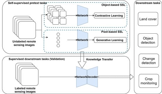
The proposed SSL framework aims to learn useful representations that keep both spatial and spectral information from label-free remote sensing data and demonstrate that such representations can be used to boost downstream remote-sensing tasks. The proposed SSL framework can be used for remote sensing analysis at both object- and pixel-level analysis:
- 1.
- The object-based SSL method (ObjSSL) employs contrastive learning. This method is suitable for extracting features from high- to very-high-spatial-resolution remote sensing data. ObjSSL employs a joint spatial–spectral-aware multiview pretext task, which is a classification problem. It uses cross-entropy loss to measure how well the network can classify the representation among a set of multiviews of a single target.
- 2.
- The pixel-based SSL method (PixSSL) employs generative learning and is suitable for low- to medium-spatial-resolution images. We propose a spectral-aware pretext task for reconstructing the original spectral profile. A spectral masked, auto encoder–decoder is designed to learn meaningful latent representations.
The framework of the proposed SSL method is shown in Figure 1. The first step is SSL training with unlabeled data; this is followed by the trained representations and network being used for downstream tasks through knowledge transfer. A specific decoder is added after the network for each specific task. We evaluate the performance of the proposed SSL framework by investigating specific downstream tasks (a multilabel land cover classification task on Sentinel-2 multispectral datasets and a ground soil parameter retrieval task on hyperspectral datasets).
3.1. Object-Based SSL (ObjSSL)
ObjSSL ia a contrastive learning method to learn the representation of remote sensing data. The idea of contrastive learning is to learn representations that bring similar data points (positive pairs) closer while pushing randomly selected points further away or to maximize the contrastive-based mutual information lower bound between different views (negative pairs). The pretext task of ObjSSL is a classification problem that uses contrastive loss to measure how well the model can classify the representation among a set of unrelated negative and positive samples. In this work, the positive samples are generated by discerning the representation of augmented views of the same data. The negative pairs assume that different images in a batch during model training represent different categories. The flowchart of the work is shown in Figure 2. There are two main parts to ObjSSL:
- 1.
- A novel multi-view pretext task that generates positive pairs for ObjSSL by generating different views of remote sensing data from both the spectral and spatial perspectives. This is a composition of multiple data augmentation operations, including spectral aware augmentation, regular augmentation, and local and global augmentation.
- 2.
- A self-distillation framework that uses two networks, a student network and a teacher network, to learn the representation from multiviews of the data. The student network is trained to match the output of a given teacher network.
3.1.1. Multiview Pretext Task
In ObjSSL, the positive pairs are generated by applying data augmentation to create noise versions of the original samples. Appropriate data augmentation is essential for learning good, generalizable embedding features. It introduces changes to the original images without modifying the semantic meaning, thus encouraging the model to learn the essential features. The author of [68] demonstrated that the composition of multiple data augmentation operations is crucial in defining the contrastive prediction tasks that yield effective representations. In this work, a joint spatial–spectral-aware multiview pretext task is proposed to generate positive pairs of data for ObjSSL. This task consists of a composite of multiple data augmentation operations, including (1) regular augmentation, (2) local and global spatial augmentation, and (3) spectral aware augmentation.
Regular Augmentation
Regular augmentation includes common data transformations, such as random rotation and zooming, Gaussian blur, and random noise.
Local and Global (LaG) Augmentation
Local and global augmentation is used to generate views of different spatial areas. With an input data X of size , the output of this augmentation is a set containing global views and several local views of smaller resolutions. We assume that the original data contains the global context. The small crops are called local views that use an image size of . This covers less than 50% of the global view but we assume that it contains the local context. Then, the two views are fed into the self-distillation framework. All local views are passed through the student network while only the global view is passed through the teacher network. This encourages the student network to interpolate context from a small cropped image and the teacher network to interpolate context from a bigger image.
Spectral Aware Augmentation
Spectral-aware augmentation is a data transformation that is performed in parallel with local and global augmentation. The traditional color-based augmentation method is a set of random transformations on random channels, including variations between channels, which inevitably change the spectral order of their relative positions. In this work, the spectral-aware augmentation process drops the random channels (30–50%) and replaces them with a value of zero. This guarantees that the relationship and relative position of the different channels do not change. This view is passed through the student encoder. This encourages the student network to learn the full spectral context from the teacher network.
3.1.2. Self-Distillation Framework
The self-distillation framework consists of teacher and student networks (encoders) that have the same structure but different parameters ( and ). In this work, the spectral–spatial vision transformer [27], designed to extract spectral and spatial features from remote sensing data, is selected as the encoder. From a given image X, we generate a set of different views (,,…) by data augmentation. and are fed into the teacher and student encoders separately and the outputs are the probability distributions and . This can be formulated as:
where g is the encoder with parameters and is a temperature parameter that controls the sharpness of the output distribution. The Softmax is used to normalize the features and allows the attention mechanism to focus on the most important information in the input. We learn to match these distributions by minimizing the cross-entropy loss between and .
In this work, the teacher is a momentum teacher, which means that the student weights ) are an exponentially moving average. The update rule for the teacher weights () is:
with following a cosine schedule from 0.96 to 1 during training. The algorithm is summarized in Algorithm 1.
| Algorithm 1 Object-Based SSL algorithm |
| Input: : One batch images; T: Teacher Network; S: Student Network; 1: set ; 2: set # Frozen Teacher’s params; 3: for x in do # One batch training 4: # Global view with regular augmentation 5: # Local view with regular augmentation 6: # Spectral mask with regular augmentation 7: 8: 9: # 10: loss.backward() # Back-propagate 11: Update(S.params) # Student params update by SGD 12: # Teacher params update by knowledge distillation 13: 14: 15: 16: loss.backward() 17: Update(S.params) 18: 19: end for |
3.2. Pixel-Based SSL (PixSSL)
PixSSL is a generative SSL method in which the pretext task is to reconstruct the original input while learning meaningful latent representation. Figure 3 shows the architecture of PixSSL. In this work, from a pixel perspective, we designed a spectral information reconstruction task to learn latent representations from the rich spectral information of remote sensing data. There are three main innovations in PixSSL:
- 1.
- To ensure that the relationships and relative positions of the different spectral channels remain unchanged, a spectral reconstructive pretext task is introduced to recover each pixel’s spectral profile from masked data. Based on our experiments, we find that masking 50% of the spectral information yields a meaningful self-supervisory task.
- 2.
- An encoder–decoder architecture is designed to perform this pretext task. The encoder is used to generate meaningful latent representation and the decoder is used to recover the masked spectral profile.
- 3.
- Pixel-based analysis methods require processing every pixel within an image, which significantly increases the amount of computation. To optimize computational efficiency, our proposed encoder can operate on a subset of the spectral data (masked data) to reduce the data input. Meanwhile, the aim of the SSL is to train an encoder to generate meaningful latent representations for downstream tasks. Therefore, we only added a lightweight decoder that reconstructs the spectral profile to reduce computational consumption.
The algorithm is summarized in Algorithm 2.
| Algorithm 2 Pixel-Based SSL algorithm |
| Input: : One batch pixels; E: Encoder Network; D: Decoder Network; 1: for x in do # One batch training 2: # Mask random spectrum, mask means masked data 3: # Forward Encoder 4: Restore the maksed data 5: # Forward Decoder 6: 7: loss.backward() # Back-propagate 8: Update(S.params) #params update 9: end for |
3.2.1. Spectral Reconstructive Pretext Task
The self-supervised pretext task in PixSSL aims to recover spectral information from masked data. In this work, we use high masking ratios to randomly mask each piece of data’s spectral profile. The high ratios largely eliminate redundancy, resulting in a pretext task that cannot be easily solved by extrapolation from visible neighboring bands. Through a PixSSL performance experiment, we found that masking 50% of the spectral information yields a meaningful latent representation.
3.2.2. The Spectral Masked Auto Encoder–Decoder Network
In this work, we have proposed a spectral-masked autoencoder that reconstructs the original spectral information given its partial spectral information. Our approach has an encoder that maps the pixel’s spectral information to a latent representation, and a decoder that reconstructs the spectral profile from the latent representation. Figure 3 illustrates the flowchart of PixSSL’s operations. We use an asymmetric design that allows the encoder to operate on masked partial spectral information, and a decoder that reconstructs the full spectral information from the latent representation and mask tokens. The last layer of the decoder is a linear projection whose number of outputs equals the number of spectral channels of the data. The loss function computes the mean squared error (MSE) between the reconstructed and original data in the pixel space.
Encoder
The encoder in this work is a transformer encoder that is applied only on unmasked data. Only 50% of the spectral channel is used for the encoder in the SSL training. Our encoder embeds patches by a linear projection with added positional embedding and then processes the resulting set via a number (N) of encoder blocks.
The encoder has four main parts, as shown in Figure 3: Multi-Head Self Attention layer (MSP), Multi-Layer Perceptrons (MLP), Layer Norm, and Residual connections, which were introduced in an evolved CNN [69].
Multi-Head Self Attention layer (MSP)
The MSP is the core of the transformer, and it consists of several self-attention blocks (h) that integrate multiple complicated interactions between different elements in the sequence (Figure 4). The self-attention mechanism can perform non-local operations, capturing long-range dependencies/global information between selected patches in the sMRI image [70]. Here, we denote the input of the model as a sequence of n patches (,…) by , where d is the embedding dimension of each patch. The goal of self-attention is to capture the interaction between all n patches by encoding each patch in terms of the global contextual information, which is done by defining three learnable weight matrices to transform Queries (), Keys (), and Values (), where . The input P is first projected into Queries (Q), Keys (K), and Values (V) by using a 1 × 1 × 1 convolution filter, which can be defined as:
The output of the self-attention layer is:
The self-attention computes the dot-product of the query with all keys, which is then normalized using the SoftMax operator to obtain the attention scores. Each patch becomes the weighted sum of all patches in the image, where the attention scores give weights.
Each self-attention block has its own learnable weight (,,,). The output of the h self-attention blocks () in multihead attention is then concatenated into a single matrix and subsequently, projected to another weight matrix . The operation is shown in Figure 4 and can be formulated as:
Then, for building a deeper model, a residual connection is employed around each module, followed by layer normalization [71]. Layer Norm is the normalization method used in NLP tasks in contrast to the batch norm approach used in vision tasks. It is applied before every block as it does not introduce any new dependencies between the training images. It helps to improve training time and generalization performance. The operation can be written as:
Multi-Layer Perceptrons (MLP)
An MLP is a particular case of a feedforward neural network where every layer is a fully connected layer. An MLP is added at the end of each MRI transformer block, containing two fully connected layers (Fc1 and Fc2) with a Gaussian Error Linear Unit (GELU). The MLP has been proven to be an essential part of the transformer as it stops and drastically slows down rank collapse in model training [72]. Residual connections are applied after every block as they allow the gradients to flow through the network directly without passing through nonlinear activations. The output of the MLP can be written as:
Decoder
The input to the decoder is the full set of tokens consisting of (i) encoded visible patches, and (ii) mask tokens. Each mask token is a shared, learned vector that indicates the presence of a missing patch to be predicted. We add positional embedding to all tokens in this full set—without this, mask tokens would have no information about their location in the image. The decoder has another series of transformer blocks. The decoder is only used during pre-training to perform the image reconstruction task (only the encoder is used to produce image representations for recognition).
4. Experiments Evaluation
This section is devoted to illustrating the capabilities of the proposed approach in two typical application scenarios and types of data. There are two main experiments: in the first experiment we evaluate the performance of ObjSSL through a downstream multilabel classification task. The most common source of medium-resolution multispectral data, the Sentinel-2 mission, is selected as the data source. In the second experiment, we measure the performance of PixSSL using hyperspectral data through a soil parametric regression task.
4.1. ObjSSL Performance Evaluation
In this work, we evaluate the performance of the proposed ObjSSL through a downstream multilabel classification task. We have conducted three types of experiments:
- 1.
- Sensitivity Analysis of the Proposed Approach. In this experiment, we analyze the sensitivity of the proposed approach under different settings and strategies. Firstly, we analyze downstream task performance with and without the spectral-aware and LaG data augmentations to evaluate the impact of the designed pretext task. Then, we report the model performance with 5%, 25%, 50%, and 100% of the training data with and without SSL to demonstrate the effect of SSL on the supervised classification task.
- 2.
- 3.
4.1.1. Data Collection
A public dataset BigEarthNet [75] is used for this experiment. A total of 125 Sentinel-2 tiles acquired between June 2017 and May 2018 from the 10 European countries (Austria, Belgium, Finland, Ireland, Kosovo, Lithuania, Luxembourg, Portugal, Serbia, and Switzerland) are initially selected. All the tiles are atmospherically corrected using the Sentinel-2 Level 2A product generation and formatting tool (sen2cor). Then, each tile is divided into non-overlapping image patches with the size of 120*120. Each image patch was annotated with the multiple land-cover classes (i.e., multilabels) provided by the CORINE Land Cover database for 2018 (CLC 2018). The CLC Level-3 nomenclature is interpreted and arranged into a new nomenclature of 19 classes (see Table 2). Ten classes of the original CLC nomenclature are maintained in the new nomenclature, 22 classes are grouped into 9 new classes, and 11 classes are removed. There are a total of 519,284 patches of data. Since the data may have been acquired in the same geographical area at different times, the result may not be reliable due to the possibility of data acquired in the same place appearing in both the training and prediction sets. To avoid this issue, the training and validation sets do not share images acquired in the same geographical area. To this end, we use the data list in [76,77]. Table 2 shows the number of images of each class associated with the training and validation sets. In this experiment, the SSL methods of both the proposed model and the existing models are trained using this data.
4.1.2. Evaluation Metrics
Evaluating the performance of a multilabel classification method requires the analysis of several factors, not just the assessment of the number of correct predictions, and, therefore, requires more complex analysis than in the single-label case. In this work, various classification-based metrics and ranking-based metrics with varying characteristics are selected to accurately evaluate the accuracy of the proposed approach. Under the category of classification-based metrics, results of experiments are provided in terms of five performance metrics: (1) Accuracy, (2) Precision, (3) Recall, (4) F1 Score, and (5) Hamming loss (HL). We also employ the receiver operating characteristic curve (ROC) and Area Under the Curve (AUC) of the ROC to evaluate classification performance. These metrics are calculated as follows:
where , , , and represent true positives, false positives, false negatives, and true negatives, respectively. We use a macro average for the overall Precision, Recall, and F1-Score. A macro average will compute the metric independently for each class and then take the average, which is preferable when there is class data imbalance.
The F1-Score is the weighted harmonic mean of the correct prediction rates among the considered ground reference and multilabel predictions.
The Hamming loss (HL) is the average Hamming distance between the ground reference labels and predicted multilabels. It penalizes the classifier for each incorrectly predicted label, regardless of the class. This makes it a more informative metric for evaluating the performance of classifiers on imbalanced datasets. It is defined as follows:
where is the predicted value for the jth label of a given sample, is the corresponding true value, and is the number of classes or labels. Under the category of ranking-based metrics, results of experiments are provided in terms of three performance evaluation metrics: (1) ranking loss (RL), (2) coverage (COV), and (3) label ranking average precision (LRAP). All the ranking-based metrics are defined with respect to the ranking of the jth label in the class probabilities result of a multilabel classification approach for the ith image that is defined as . Unlike the classification-based metrics, ranking-based metrics are calculated only by giving equal importance to each sample of the test set.
Accordingly, ranking loss (RL) is the rate of wrongly ordered label pairs (i.e., the probability of a label, which is irrelevant to the image, is higher than a ground reference label), and thus, is expressed as follows:
The coverage (COV) calculates the average number of labels required to be included in the prediction list of a multilabel classifier such that all ground reference labels will be predicted. Accordingly, it is defined as follows:
For each ground reference label, the label ranking average precision (LRAP) calculates the rate of higher-ranked ground reference labels. This is expressed as follows:
It is worth noting that, smaller values of the Hamming loss, ranking loss, and coverage, but higher values of the accuracy, precision, recall, F1-Score, and the LRAP, are associated with better performance.
4.1.3. Experimental Setup
The model training in this work has two main steps. The first is SSL training without labels. The second is supervised training. We can choose either the SSL-generated weights or the default weights as the initial weights.
The SSL training uses the AdamW optimizer [78] and a batch size of 64, distributed over three GPUs (GeForce RTX 2080 Ti). An efficient training strategy for SSL is used in this work [79]. The learning rate is linearly ramped up during the first 10 epochs as 1 × 10. After this warm-up, we decay the learning rate with a cosine schedule. The weight decay also follows a cosine scheduled from 0.04 to 0.4. The cosine decay scheduler starts with a high learning rate and then decreases it in a cosine wave pattern. This means that the learning rate decreases quickly at first and then more slowly as the model approaches convergence. This helps to ensure that the model learns quickly in the early stages of training and then fine-tunes its parameters in the later stages of training. We execute training for 100 epochs.
For the supervised training, we first transfer the weights learned from SSL training to initialize the model. An AdamW optimizer is used for 100 epochs using a cosine decay learning rate scheduler and 20 epochs of linear warm-up. A batch size of 64, a lower initial learning rate of 1 × 10, and a weight decay of 0.05 are used for model training. The binary cross-entropy (BCE) loss, which is a measure of the difference between two probability distributions, is used as the loss function. BCE loss is well-suited for multilabel classification because it can be applied to each label independently.
4.2. PixSSL Performance Evaluation
In this work, we evaluate the performance of the proposed PixSSL through a downstream parameter regression task using a hyperspectral dataset. The objective of the task is to estimate soil parameters, specifically, potassium (K), phosphorus pentoxide (PO), magnesium (Mg), and pH, from hyperspectral images captured over agricultural areas in Poland. The dataset and task design are from a public competition, the AI4EO hyperspectral challenge [80].
4.2.1. Data Collection
The dataset comprises 2886 patches (2 m GSD), of which 1732 are used for training and 1154 for evaluation. The patch size varies (depending on agricultural parcels) and is on average around 60 × 60 pixels. Each patch contains 150 contiguous hyperspectral bands (462–942 nm, with a spectral resolution of 3.2 nm). Figure 5 shows the data representation of band 60 and the spectral profile of one patch.
4.2.2. Experimental Setup
Two experiments are carried out to evaluate the performance of PixSSL. The first determines the best masking ratio. The second is a comparative experiment. Three existing methods are selected for comparison.
The baseline method is the machine learning pixel-based method. We assume that each patch is treated as a pixel and average all the values of each waveband in this patch. The spectral profile of each patch is used as the input. The catboost [81] model, as one of the state-of-the-art machine learning regression models, is selected for regression.
The root mean squared error (RMSE) and the R-squared () scores are used to evaluate the model’s performance. In the baseline model, 1732 spectral profiles are extracted from the patch and used for model training. Then, we perform PixSSL on all datasets. We extract around 400 spectral profiles (from 3 × 3 area) from one patch (60 × 60 pixels). So 1732 × 400 = 692,800 are used for the pre-training without labels. Finally, we perform the downstream regression task to evaluate the representations using two methods: linear probing and fine-tuning (Figure 6).
In linear probing (SSL_LP), a decoder (linear layer) is stacked on top of the encoder and only the decoder is trained by accessing the labels. Since the encoders have already been trained in the first stage, we freeze all the parameters of the encoder in the downstream task training.
In fine-tuning (SSL_FT), a similar procedure is followed. In the first stage, encoders are trained without accessing the labels and all the parameters are used as initialization in the second stage. In the second stage, a decoder is stacked on top of the backbone, and the whole model is trained by accessing the labels. Notice that we use a smaller learning rate on the encoder to avoid large shifts in weight space.
For the SSL pre-training, we use the AdamW optimizer and a batch size of 512, distributed over three GPUs (GeForce RTX 2080 Ti). The learning rate is based on a scaling rule [82]:
After this warm-up, we decay the learning rate with a cosine schedule. The weight decay also follows a cosine schedule from 0.04 to 0.4. For the supervised training on the downstream regression task, we first transfer the weights learned from SSL to initialize the model. An AdamW optimizer is used for 100 epochs using a cosine decay learning rate scheduler and 20 epochs of linear warm-up. This learning rate scheduler is only applied to the decoder and a lower learning rate (1 × 10) is applied to the encoder.
5. Results
In this section, we report the performance of proposed method according to the object-based (ObjSSL) and pixel-based (PixSSL) remote sensing data analysis methods. In the ObjSSL performance experiments, we first perform sensitivity analyses to report the impact of our proposed structure on model performance (Section 5.1.1), and then report the results of the comparison with current commonly used SSL methods (Section 5.1.2) and deep learning structures (Section 5.1.3). In the PixSSL performance experiments (Section 5.2), we first report the parameter selection in this method and then report the performance of the proposed SSL method.
5.1. ObjSSL Performance
5.1.1. Sensitivity Analysis of the Proposed Approach
In this section, we first evaluate the impact of spectral-aware data augmentation on SSL. The impact of our proposed augmentation methods (spectral-aware and LaG augmentation) on model performance are shown in Table 3. By analyzing the results, one can see that the model using the all augmentations achieves the highest score for each class. The average Precision, Recall, and F1 scores of the proposed SSL method are 78.66%, 66.52%, and 71.10%, which are 5.64%, 4.40%, and 5.05% higher than the model without spectral-aware augmentation and 13.08%, 8.72%, and 10.14% higher than the model without both spectral-aware and LaG augmentations. This result demonstrates that spectral information in remote sensing data plays a key role in ground object classification.
One of the motivations of SSL is to learn useful representations of data from unlabeled data and then fine-tune the representations with a few labels for the supervised downstream task. In this task, we evaluate the effect of SSL processing in the downstream task, especially when the amount of training data is limited. Figure 7 shows the model performance with 5%, 25%, 50%, and 100% of the training data. The results show that the accuracy of supervised classification on the validation dataset drops significantly when less than 50% of the data is used for training. The F1 score and LRAP are only 22.4% and 32.4%, respectively, when using 5% of the training data. This indicates that the model is overfitting. When using SSL weights for fine-tuning, the model can achieve its maximum accuracy using only 5% of the training data.
5.1.2. Comparison with Existing SSL Frameworks
In the second experiment, we compare the classification results of different existing SLL frameworks with our proposed method. We pre-train the model with four SSL frameworks (MoCo-V2 [58], BYOL [51], DINO [50], and the proposed SSL framework) and then fine-tune the representations on 50% of the training data. Table 4 shows the model performance results with the model performance results without SSL added as a reference. The results show that the use of SSL can be beneficial in allowing the model to converge on limited data. Compared to the three existing SSL frameworks, the proposed SSL method emphasizes the spectral and spatial features in remote sensing data with better performance. Figure 8 shows the ROC with AUC obtained by the proposed method and the three existing SSL methods. The AUC of our proposed method is 0.97, which is higher than those of the other SSLs, which range from 0.945 to 0.935.
5.1.3. Comparison with Existing Networks
Table 5 shows the classification-based and rank-based metrics obtained by the proposed method and the three most popular deep learning networks: VGG16, ResNet50, and ViT. Since the BigEearthNet dataset collects 393,000 pieces of training data, it is sufficient for most visual tasks. All the deep learning models achieve satisfactory accuracy on supervised tasks. Duo to the residual connection approach introduced by ResNet [69], ResNet obtains a superior accuracy than VGG16, which is also demonstrated in most computer vision tasks [83]. ViT [74], a new computer vision architecture that utilizes a transformer instead of a CNN to extract features of the data, achieves accuracy performance close to that of VGG16. Our method introduces a channel information learning module into VIT, and shows better performance than ResNet and VIT. A minor improvement in accuracy is also obtained with the addition of SSL in both classification-based and rank-based metrics.
5.2. PixSSL Performance
Figure 9 shows the influence of the masking ratio. The results show that the ratio of 50% is the best option for self-supervised representation learning in this task.
In this section, we evaluate the performance of PixSSL on a downstream regression task. Figure 10 shows the and RMSE accuracy of the baseline method and proposed SSL method. With the traditional machine learning pixel-based method, the of nitrogen parameter prediction is around 0.85. With the SSL representation, the of the SSL_LP increases from 0.93 to 0.95 for P, K, and Mg regressions. There is no significant improvement in pH regression since the values of pH on the ground target are close. When we fine-tune the final layer of the encoder, the of the proposed model is improved to over 0.95. The result indicates that the representations learned from SSL provide a better prediction of nitrogen properties than using the original spectral information only.
6. Discussion
In this work, we propose an SSL framework for feature extraction of remote sensing data at both the pixel-based and object-based scales. By validating downstream tasks, our results demonstrate that the new representation of the data learned by the SSL can achieve better performance on downstream tasks than using original data only. In general, the representations learned by the SSL are abstract and cannot be interpreted directly. In the following section, we visualize the representations and discuss their potential value.
6.1. The Representation of ObjSSL
In ObjSSL, a novel multiview pretext task is proposed to generate representations from unlabeled data. In our experiments, we demonstrate that our proposed unsupervised learning method exhibits three main advantages: (1) With the joint spatial–spectral-aware pretext task, the deep learning model obtains both spectral and spatial features from the remote sensing data. The classification performance of some spectrum-sensitive categories, such as Mixed Forest, Coniferous Forest, Natural grassland and sparsely vegetated areas, Wetlands, and Arable land, has been significantly improved. (2) The representations generated from self-supervised learning improve the performance of downstream tasks. (3) After pre-training with self-supervised learning, the deep learning model can converge faster and better in supervised training with a limited dataset. This shows that self-supervised learning generalizes well to the spectral–spatial features in the data.
In Figure 11, we visualize the attention maps for the different heads of the last layer of the encoder after ObjSSL. The (a) column is the original data displayed by red, green, and blue channels. In the (b) column, we adjust the brightness of the image for better display. The (c) and (d) columns visualize the different attention maps of the last layer in the encoder after ObjSSL. The results show that the attention map can attend to different semantic regions of an image, which demonstrates that the representations obtained by SSL reflect the semantic information of the data. We believe that this representation has the potential to be used in land cover/use tasks.
In Figure 12, we represent each BigEarthNet class by using the average feature vector for its validation data. We run t-SNE for 5000 iterations and present the resulting class embedding in Figure 10. The result shows that the representation learned by ObjSSL recovers structures between classes, and similar ground objects are grouped: the water-related classes, such as inland (17) and marine waters (18), are at the bottom; broad-leaved forests (8), Coniferous forests (9), and mixed forests (10) are grouped in the middle; natural grassland and sparsely vegetated areas (11), Moors, heathland, and sclerophyllous vegetation (12), Transitional woodland, shrub (13), beaches, dunes, sand (14), and inland wetlands (15) are grouped in the top right; and arable land (2) and permanent crops (3) are on the left.
6.2. The Representation of PixSSL
In PixSSL, a reconstruction pretext task is proposed to generate representations from unlabeled data. Our experimental results demonstrate that the representations obtained by SSL can significantly improve the accuracy of pixel-based analysis tasks. In Figure 13, we display how PixSSL reconstructs the masked spectrum. The (a) column shows the original spectral profile, the (b) column shows the masked spectral profile where 50% of the data are masked, and the (c) column shows the reconstructions of the spectral information. The first two rows show the spectral information of vegetation, and the third row shows bare soil. As can be seen from the results, despite 50% of the data being masked, PixSSL recovers the spectral curve well. It can be concluded that PixSSL learns the spectral features from massive unlabeled data very well.
6.3. Challenges and Future Directions
In this work, we have demonstrated that SSL learning can enhance the performance of remote sensing applications with remarkable efficiency, by greatly reducing the dependence of deep models on large amounts of annotated data. Nevertheless, as an emerging field within computer vision, it still faces the following hurdles.
(1) Computing efficiency. SSL usually requires significant computational resources due to the large amount of pre-trained data, complex and varied data enhancements, large batch size of training data and more training epochs than other existing supervised learning methods, etc. Meanwhile, with the growth in popularity of hyper NPL model, such as BERT [84], ChatGPT [85], LaMDA [86], etc. SSL is also widely used to train mega models, which poses a serious challenge to computational resources. To date, there have been some efforts to reduce the cost of SSL computing [87,88,89], but few cases have been used for remote sensing applications. The effective remote sensing data loading, especially for multi/hyperspectral data, model design, parallel computing, and hardware acceleration are, therefore, still to be explored.
(2) Prompt Engineering, also known as contextual prompting, refers to methods for communicating with large deep learning models to guide their behavior towards desired outcomes without updating their weights [90,91,92]. Self-supervised learning often requires tremendous computational resources to train large models, which poses challenges for non-enterprise researchers. Prompt engineering is an empirical science and does not require large computational resources. The effectiveness of prompt engineering methods can vary considerably between models, and, therefore, good performance requires a lot of experience and experimentation. Remote sensing engineering has a vast amount of empirical research and pattern recognition in recent decades, and it is reasonable to believe that this accumulated knowledge can be used to accelerate the convergence of SSL models.
(3) The generalizability of SSL models on remote sensing data. Unlike conventional color digital images, which usually have three bands, RGB, remote sensing data usually have multiple bands, the number of which depend on the sensor. This leads to inconsistencies in the format of remotely sensed data. In this work, we used Sentinel-2 multispectral and I4EO hyperspectral data for SSL training and evaluated the model on the same data. Because of the difference in band properties, these models cannot be used directly with other remote sensing data, which limits the generalizability of the models. The development of SSL models for multisource remote sensing data, adapted to different band configurations, will be a future research direction.
7. Conclusions
In this work, we have proposed a generic self-supervised learning framework based on remote sensing data at both the object and pixel levels. This proposed SSL method learns a target representation that covers both spatial and spectral information from massive unlabeled data. Use of this representation as input has been shown to achieve superior performance in downstream remote sensing tasks than using original data as input. More importantly, this approach can alleviate the problem of the time and labor cost of labeling remote sensing data for use with traditional supervised learning. In this paper, we have designed two experiments with real data. One is land cover classification task based on Sentinel-2 multispectral datasets, for which we have selected an object-based analysis approach, and the results demonstrate that our proposed ObjSSL method outperforms traditional SSL methods that are not designed for both spectral and spatial feature extraction. The other experiment is a ground soil parameter retrieval task on hyperspectral datasets. For this, we have selected a pixel-based analysis method to utilize the rich spectral information. The results demonstrate that the proposed PixSSL can learn improved spectral representations by recovering the spectral information from the masked data. Simultaneously, we visualize the learned representation of the proposed SSL, and the results show that our SSL can learn representations from both the spectral and spatial information of unlabeled datasets. We believe that this approach has the potential to be effective in a wider range of remote sensing applications and we will explore its utility in more remote sensing applications in the future.
Author Contributions
Conceptualization, X.Z. and L.H.; methodology, X.Z. and L.H.; software, X.Z.; validation, X.Z.; formal analysis, X.Z.; investigation, L.H.; resources, L.H.; data curation, X.Z.; writing—original draft preparation, X.Z.; writing—review and editing, L.H.; visualization, X.Z.; supervision, L.H.; project administration, L.H.; funding acquisition, L.H. All authors have read and agreed to the published version of the manuscript.
Funding
This work is supported by the BBSRC (projects BB/R019983/1 and BB/S020969/1).
Data Availability Statement
Publicly available datasets were analyzed in this study.
Conflicts of Interest
The authors declare no conflict of interest.
References
- Ban, Y.; Gong, P.; Giri, C. Global Land Cover Mapping Using Earth Observation Satellite Data: Recent Progresses and Challenges. ISPRS J. Photogramm. Remote Sens. 2015, 103, 1–6. [Google Scholar] [CrossRef]
- Li, D.; Zhang, P.; Chen, T.; Qin, W. Recent Development and Challenges in Spectroscopy and Machine Vision Technologies for Crop Nitrogen Diagnosis: A Review. Remote Sens. 2020, 12, 2578. [Google Scholar] [CrossRef]
- Osco, L.P.; Marcato Junior, J.; Marques Ramos, A.P.; de Castro Jorge, L.A.; Fatholahi, S.N.; de Andrade Silva, J.; Matsubara, E.T.; Pistori, H.; Gonçalves, W.N.; Li, J. A review on deep learning in UAV remote sensing. Int. J. Appl. Earth Obs. Geoinf. 2021, 102, 102456. [Google Scholar] [CrossRef]
- Ghamisi, P.; Plaza, J.; Chen, Y.; Li, J.; Plaza, A.J. Advanced Spectral Classifiers for Hyperspectral Images: A review. IEEE Geosci. Remote Sens. Mag. 2017, 5, 8–32. [Google Scholar] [CrossRef]
- Richards, J.A. Remote Sensing Digital Image Analysis; Springer: Berlin/Heidelberg, Germany, 2006. [Google Scholar]
- Chen, G.; Weng, Q.; Hay, G.J.; He, Y. Geographic object-based image analysis (GEOBIA): Emerging trends and future opportunities. GISci. Remote Sens. 2018, 55, 159–182. [Google Scholar] [CrossRef]
- Pal, M.; Mather, P.M. An assessment of the effectiveness of decision tree methods for land cover classification. Remote Sens. Environ. 2003, 86, 554–565. [Google Scholar] [CrossRef]
- Cortes, C.; Vapnik, V. Support-vector networks. Mach. Learn. 1995, 20, 273–297. [Google Scholar] [CrossRef]
- Breiman, L. Random Forests. Mach. Learn. 2001, 45, 5–32. [Google Scholar] [CrossRef]
- Pal, M. Random forest classifier for remote sensing classification. Int. J. Remote Sens. 2005, 26, 217–222. [Google Scholar] [CrossRef]
- Safari, A.; Sohrabi, H.; Powell, S.; Shataee, S. A comparative assessment of multi-temporal Landsat 8 and machine learning algorithms for estimating aboveground carbon stock in coppice oak forests. Int. J. Remote Sens. 2017, 38, 6407–6432. [Google Scholar] [CrossRef]
- Singh, C.; Karan, S.K.; Sardar, P.; Samadder, S.R. Remote sensing-based biomass estimation of dry deciduous tropical forest using machine learning and ensemble analysis. J. Environ. Manag. 2022, 308, 114639. [Google Scholar] [CrossRef]
- Garcia-Garcia, A.; Orts-Escolano, S.; Oprea, S.; Villena-Martinez, V.; Garcia-Rodriguez, J. A Review on Deep Learning Techniques Applied to Semantic Segmentation. arXiv 2017, arXiv:1704.06857. [Google Scholar]
- Zhang, X.; Han, L.; Han, L.; Zhu, L. How Well Do Deep Learning-Based Methods for Land Cover Classification and Object Detection Perform on High Resolution Remote Sensing Imagery? Remote Sens. 2020, 12, 417. [Google Scholar] [CrossRef]
- Ball, J.E.; Anderson, D.T.; Chan, C.S. A Comprehensive Survey of Deep Learning in Remote Sensing: Theories, Tools and Challenges for the Community. J. Appl. Remote Sens. 2017, 11, 1. [Google Scholar] [CrossRef]
- Romero, A.; Gatta, C.; Camps-Valls, G. Unsupervised Deep Feature Extraction for Remote Sensing Image Classification. IEEE Trans. Geosci. Remote Sens. 2016, 54, 1349–1362. [Google Scholar] [CrossRef]
- Hatano, T.; Tsuneda, T.; Suzuki, Y.; Shintani, K.; Yamane, S. Image Classification with Additional Non-decision Labels using Self-supervised learning and GAN. In Proceedings of the IEEE 2020 Eighth International Symposium on Computing and Networking Workshops (CANDARW), Naha, Japan, 24–27 November 2020; pp. 125–129. [Google Scholar]
- Li, Y.; Chen, J.; Zheng, Y. A multi-task self-supervised learning framework for scopy images. In Proceedings of the 2020 IEEE 17th International Symposium on Biomedical Imaging (ISBI), Iowa City, IA, USA, 3–7 April 2020; pp. 2005–2009. [Google Scholar]
- Lan, Z.; Chen, M.; Goodman, S.; Gimpel, K.; Sharma, P.; Soricut, R. Albert: A lite bert for self-supervised learning of language representations. arXiv 2019, arXiv:1909.11942. [Google Scholar]
- Leiter, C.; Zhang, R.; Chen, Y.; Belouadi, J.; Larionov, D.; Fresen, V.; Eger, S. ChatGPT: A Meta-Analysis after 2.5 Months. arXiv 2023, arXiv:2302.13795. [Google Scholar] [CrossRef]
- Misra, I.; van der Maaten, L. Self-supervised learning of pretext-invariant representations. In Proceedings of the IEEE/CVF Conference on Computer Vision and Pattern Recognition, Seattle, WA, USA, 13–19 June 2020; pp. 6707–6717. [Google Scholar]
- Mitash, C.; Bekris, K.E.; Boularias, A. A self-supervised learning system for object detection using physics simulation and multi-view pose estimation. In Proceedings of the 2017 IEEE/RSJ International Conference on Intelligent Robots and Systems (IROS), Vancouver, BC, Canada, 24–28 September 2017; pp. 545–551. [Google Scholar]
- Alosaimi, N.; Alhichri, H.; Bazi, Y.; Ben Youssef, B.; Alajlan, N. Self-supervised learning for remote sensing scene classification under the few shot scenario. Sci. Rep. 2023, 13, 433. [Google Scholar] [CrossRef]
- Tao, C.; Qi, J.; Lu, W.; Wang, H.; Li, H. Remote Sensing Image Scene Classification With Self-Supervised Paradigm Under Limited Labeled Samples. IEEE Geosci. Remote Sens. Lett. 2022, 19, 1–5. [Google Scholar] [CrossRef]
- Zhao, Z.; Luo, Z.; Li, J.; Chen, C.; Piao, Y. When Self-Supervised Learning Meets Scene Classification: Remote Sensing Scene Classification Based on a Multitask Learning Framework. Remote Sens. 2020, 12, 3276. [Google Scholar] [CrossRef]
- Dong, H.; Ma, W.; Wu, Y.; Zhang, J.; Jiao, L. Self-Supervised Representation Learning for Remote Sensing Image Change Detection Based on Temporal Prediction. Remote Sens. 2020, 12, 1868. [Google Scholar] [CrossRef]
- Zhang, X.; Han, L.; Sobeih, T.; Lappin, L.; Lee, M.A.; Howard, A.; Kisdi, A. The Self-Supervised Spectral–Spatial Vision Transformer Network for Accurate Prediction of Wheat Nitrogen Status from UAV Imagery. Remote Sens. 2022, 14, 1400. [Google Scholar] [CrossRef]
- He, K.; Chen, X.; Xie, S.; Li, Y.; Dollár, P.; Girshick, R. Masked Autoencoders Are Scalable Vision Learners. arXiv 2021, arXiv:2111.06377. [Google Scholar]
- Komodakis, N.; Gidaris, S. Unsupervised representation learning by predicting image rotations. In Proceedings of the International Conference on Learning Representations (ICLR), Vancouver, BC, Canada, 30 April–3 May 2018. [Google Scholar]
- Imani, M.; Ghassemian, H. An overview on spectral and spatial information fusion for hyperspectral image classification: Current trends and challenges. Inf. Fusion 2020, 59, 59–83. [Google Scholar] [CrossRef]
- Fauvel, M.; Chanussot, J.; Benediktsson, J.A.; Sveinsson, J.R. Spectral and spatial classification of hyperspectral data using SVMs and morphological profiles. In Proceedings of the 2007 IEEE International Geoscience and Remote Sensing Symposium, Barcelona, Spain, 23–27 July 2007; pp. 4834–4837. [Google Scholar] [CrossRef]
- Lee, W.; Park, B.; Han, K. Svm-based classification of diffusion tensor imaging data for diagnosing alzheimer’s disease and mild cognitive impairment. In Proceedings of the International Conference on Intelligent Computing, Harbin, China, 17–18 January 2015; Springer: Berlin/Heidelberg, Germany, 2015; pp. 489–499. [Google Scholar]
- Belgiu, M.; Drăguţ, L. Random forest in remote sensing: A review of applications and future directions. ISPRS J. Photogramm. Remote Sens. 2016, 114, 24–31. [Google Scholar] [CrossRef]
- Chasmer, L.; Hopkinson, C.; Veness, T.; Quinton, W.; Baltzer, J. A decision-tree classification for low-lying complex land cover types within the zone of discontinuous permafrost. Remote Sens. Environ. 2014, 143, 73–84. [Google Scholar] [CrossRef]
- Friedl, M.A.; Brodley, C.E. Decision tree classification of land cover from remotely sensed data. Remote Sens. Environ. 1997, 61, 399–409. [Google Scholar] [CrossRef]
- Ball, J.E.; Anderson, D.T.; Chan, C.S. Special Section Guest Editorial: Feature and Deep Learning in Remote Sensing Applications. J. Appl. Remote Sens. 2018, 11, 1. [Google Scholar] [CrossRef]
- Ellouze, A.; Ksantini, M.; Delmotte, F.; Karray, M. Multiple Object Tracking: Case of Aircraft Detection and Tracking. In Proceedings of the IEEE 2019 16th International Multi-Conference on Systems, Signals & Devices (SSD), Istanbul, Turkey, 21–24 March 2019; pp. 473–478. [Google Scholar]
- Brown, C.F.; Brumby, S.P.; Guzder-Williams, B.; Birch, T.; Hyde, S.B.; Mazzariello, J.; Czerwinski, W.; Pasquarella, V.J.; Haertel, R.; Ilyushchenko, S.; et al. Dynamic World, Near real-time global 10 m land use land cover mapping. Sci. Data 2022, 9, 251. [Google Scholar] [CrossRef]
- Wang, Y.; Albrecht, C.M.; Braham, N.A.A.; Mou, L.; Zhu, X.X. Self-Supervised Learning in Remote Sensing: A review. IEEE Geosci. Remote Sens. Mag. 2022, 10, 213–247. [Google Scholar] [CrossRef]
- Bruzzone, L.; Prieto, D.F. Unsupervised retraining of a maximum likelihood classifier for the analysis of multitemporal remote sensing images. IEEE Trans. Geosci. Remote Sens. 2001, 39, 456–460. [Google Scholar] [CrossRef]
- Congalton, R.G. A review of assessing the accuracy of classifications of remotely sensed data. Remote Sens. Environ. 1991, 37, 35–46. [Google Scholar] [CrossRef]
- Ball, G.H.; Hall, J. ISODATA: A Novel Method for Data Analysis and Pattern Classification; Stanford Research Institute: Menlo Park, CA, USA, 1965. [Google Scholar]
- Kanungo, T.; Mount, D.; Netanyahu, N.; Piatko, C.; Silverman, R.; Wu, A. An efficient k-means clustering algorithm: Analysis and implementation. IEEE Trans. Pattern Anal. Mach. Intell. 2002, 24, 881–892. [Google Scholar] [CrossRef]
- Zhang, X.; Zhang, M.; Zheng, Y.; Wu, B. Crop Mapping Using PROBA-V Time Series Data at the Yucheng and Hongxing Farm in China. Remote Sens. 2016, 8, 915. [Google Scholar] [CrossRef]
- Zhang, H.; Zhai, H.; Zhang, L.; Li, P. Spectral–spatial sparse subspace clustering for hyperspectral remote sensing images. IEEE Trans. Geosci. Remote Sens. 2016, 54, 3672–3684. [Google Scholar] [CrossRef]
- Doersch, C.; Gupta, A.; Efros, A.A. Unsupervised visual representation learning by context prediction. In Proceedings of the IEEE International Conference on Computer Vision, Santiago, Chile, 7–13 December 2015; pp. 1422–1430. [Google Scholar]
- Noroozi, M.; Favaro, P. Unsupervised learning of visual representations by solving jigsaw puzzles. In Proceedings of the European Conference on Computer Vision, Amsterdam, The Netherlands, 11–14 October 2016; Springer: Berlin/Heidelberg, Germany, 2016; pp. 69–84. [Google Scholar]
- Alexey, D.; Fischer, P.; Tobias, J.; Springenberg, M.R.; Brox, T. Discriminative, unsupervised feature learning with exemplar convolutional, neural networks. IEEE TPAMI 2016, 38, 1734–1747. [Google Scholar] [CrossRef]
- Arora, S.; Khandeparkar, H.; Khodak, M.; Plevrakis, O.; Saunshi, N. A Theoretical Analysis of Contrastive Unsupervised Representation Learning. arXiv 2019, arXiv:1902.09229. [Google Scholar]
- Caron, M.; Touvron, H.; Misra, I.; Jégou, H.; Mairal, J.; Bojanowski, P.; Joulin, A. Emerging Properties in Self-Supervised Vision Transformers. arXiv 2021, arXiv:2104.14294. [Google Scholar]
- Grill, J.B.; Strub, F.; Altché, F.; Tallec, C.; Richemond, P.H.; Buchatskaya, E.; Doersch, C.; Pires, B.A.; Guo, Z.D.; Azar, M.G.; et al. Bootstrap your own latent: A new approach to self-supervised Learning. arXiv 2020, arXiv:2006.07733. [Google Scholar]
- Vincent, P.; Larochelle, H.; Lajoie, I.; Bengio, Y.; Manzagol, P.A.; Bottou, L. Stacked denoising autoencoders: Learning useful representations in a deep network with a local denoising criterion. J. Mach. Learn. Res. 2010, 11, 3371–3408. [Google Scholar]
- Goodfellow, I.; Pouget-Abadie, J.; Mirza, M.; Xu, B.; Warde-Farley, D.; Ozair, S.; Courville, A.; Bengio, Y. Generative Adversarial Nets. In Advances in Neural Information Processing Systems 27; Ghahramani, Z., Welling, M., Cortes, C., Lawrence, N.D., Weinberger, K.Q., Eds.; Curran Associates, Inc.: Red Hook, NY, USA, 2014; pp. 2672–2680. [Google Scholar]
- Arjovsky, M.; Chintala, S.; Bottou, L. Wasserstein GAN. arXiv 2017, arXiv:1701.07875. [Google Scholar]
- Chen, X.; Fan, H.; Girshick, R.; He, K. Improved baselines with momentum contrastive learning. arXiv 2020, arXiv:2003.04297. [Google Scholar]
- Chen, X.; Xie, S.; He, K. An Empirical Study of Training Self-Supervised Vision Transformers. arXiv 2021, arXiv:2104.02057. [Google Scholar]
- He, K.; Fan, H.; Wu, Y.; Xie, S.; Girshick, R. Momentum contrast for unsupervised visual representation learning. In Proceedings of the IEEE/CVF Conference on Computer Vision and Pattern Recognition, Seattle, WA, USA, 13–19 June 2020; pp. 9729–9738. [Google Scholar]
- Chen, X.; He, K. Exploring Simple Siamese Representation Learning. arXiv 2020, arXiv:2011.10566. [Google Scholar] [CrossRef]
- Wen, Z.; Liu, Z.; Zhang, S.; Pan, Q. Rotation awareness based self-supervised learning for SAR target recognition with limited training samples. IEEE Trans. Image Process. 2021, 30, 7266–7279. [Google Scholar] [CrossRef] [PubMed]
- Singh, S.; Batra, A.; Pang, G.; Torresani, L.; Basu, S.; Paluri, M.; Jawahar, C.V. Self-Supervised Feature Learning for Semantic Segmentation of Overhead Imagery. In Proceedings of the BMVC, Newcastle upon Tyne, UK, 3–6 September 2018; Volume 1, p. 4. [Google Scholar]
- Geng, W.; Zhou, W.; Jin, S. Multi-view urban scene classification with a complementary-information learning model. Photogramm. Eng. Remote Sens. 2022, 88, 65–72. [Google Scholar] [CrossRef]
- Rao, W.; Qu, Y.; Gao, L.; Sun, X.; Wu, Y.; Zhang, B. Transferable network with Siamese architecture for anomaly detection in hyperspectral images. Int. J. Appl. Earth Obs. Geoinf. 2022, 106, 102669. [Google Scholar] [CrossRef]
- Zhang, L.; Lu, W.; Zhang, J.; Wang, H. A Semisupervised Convolution Neural Network for Partial Unlabeled Remote-Sensing Image Segmentation. IEEE Geosci. Remote Sens. Lett. 2022, 19, 1–5. [Google Scholar] [CrossRef]
- Jean, N.; Wang, S.; Samar, A.; Azzari, G.; Lobell, D.; Ermon, S. Tile2Vec: Unsupervised representation learning for spatially distributed data. arXiv 2018, arXiv:1805.02855. [Google Scholar] [CrossRef]
- Hou, S.; Shi, H.; Cao, X.; Zhang, X.; Jiao, L. Hyperspectral imagery classification based on contrastive learning. IEEE Trans. Geosci. Remote Sens. 2021, 60, 1–13. [Google Scholar] [CrossRef]
- Duan, P.; Xie, Z.; Kang, X.; Li, S. Self-supervised learning-based oil spill detection of hyperspectral images. Sci. China Technol. Sci. 2022, 65, 793–801. [Google Scholar] [CrossRef]
- Zhu, M.; Fan, J.; Yang, Q.; Chen, T. SC-EADNet: A Self-Supervised Contrastive Efficient Asymmetric Dilated Network for Hyperspectral Image Classification. IEEE Trans. Geosci. Remote Sens. 2022, 60, 1–17. [Google Scholar] [CrossRef]
- Chen, T.; Kornblith, S.; Norouzi, M.; Hinton, G. A Simple Framework for Contrastive Learning of Visual Representations. arXiv 2020, arXiv:2002.05709. [Google Scholar]
- He, K.; Zhang, X.; Ren, S.; Sun, J. Deep Residual Learning for Image Recognition. arXiv 2015, arXiv:1512.03385. [Google Scholar]
- Buades, A.; Coll, B.; Morel, J.M. A non-local algorithm for image denoising. In Proceedings of the 2005 IEEE Computer Society Conference on Computer Vision and Pattern Recognition (CVPR’05), San Diego, CA, USA, 20–25 June 2005; Volume 2, pp. 60–65. [Google Scholar]
- Ba, J.L.; Kiros, J.R.; Hinton, G.E. Layer Normalization. arXiv 2016, arXiv:1607.06450. [Google Scholar]
- Dong, Y.; Cordonnier, J.B.; Loukas, A. Attention is Not All You Need: Pure Attention Loses Rank Doubly Exponentially with Depth. arXiv 2021, arXiv:2103.03404. [Google Scholar]
- Simonyan, K.; Zisserman, A. Very deep convolutional networks for large-scale image recognition. arXiv 2014, arXiv:1409.1556. [Google Scholar]
- Dosovitskiy, A.; Beyer, L.; Kolesnikov, A.; Weissenborn, D.; Zhai, X.; Unterthiner, T.; Dehghani, M.; Minderer, M.; Heigold, G.; Gelly, S.; et al. An Image is Worth 16x16 Words: Transformers for Image Recognition at Scale. arXiv 2020, arXiv:2010.11929. [Google Scholar]
- Sumbul, G.; De Wall, A.; Kreuziger, T.; Marcelino, F.; Costa, H.; Benevides, P.; Caetano, M.; Demir, B.; Markl, V. BigEarthNet-MM: A Large-Scale, Multimodal, Multilabel Benchmark Archive for Remote Sensing Image Classification and Retrieval [Software and Data Sets]. IEEE Geosci. Remote Sens. Mag. 2021, 9, 174–180. [Google Scholar] [CrossRef]
- Sumbul, G.; Kang, J.; Kreuziger, T.; Marcelino, F.; Costa, H.; Benevides, P.; Caetano, M.; Demir, B. Bigearthnet deep learning models with a new class-nomenclature for remote sensing image understanding. arXiv 2020, arXiv:2001.06372. [Google Scholar]
- Sumbul, G.; Demİr, B. A Deep Multi-Attention Driven Approach for Multi-Label Remote Sensing Image Classification. IEEE Access 2020, 8, 95934–95946. [Google Scholar] [CrossRef]
- Loshchilov, I.; Hutter, F. Decoupled Weight Decay Regularization. arXiv 2017, arXiv:1711.05101. [Google Scholar]
- Koçyiğit, M.T.; Hospedales, T.M.; Bilen, H. Accelerating Self-Supervised Learning via Efficient Training Strategies. In Proceedings of the IEEE/CVF Winter Conference on Applications of Computer Vision, Waikoloa, HI, USA, 3–7 January 2023; pp. 5654–5664. [Google Scholar]
- Nalepa, J.; Le Saux, B.; Longépé, N.; Tulczyjew, L.; Myller, M.; Kawulok, M.; Smykala, K.; Gumiela, M. The Hyperview Challenge: Estimating Soil Parameters from Hyperspectral Images. In Proceedings of the 2022 IEEE International Conference on Image Processing (ICIP), Bordeaux, France, 16–19 October 2022; pp. 4268–4272. [Google Scholar] [CrossRef]
- Prokhorenkova, L.; Gusev, G.; Vorobev, A.; Dorogush, A.V.; Gulin, A. CatBoost: Unbiased boosting with categorical features. arXiv 2019, arXiv:1706.09516. [Google Scholar]
- Goyal, P.; Dollár, P.; Girshick, R.; Noordhuis, P.; Wesolowski, L.; Kyrola, A.; Tulloch, A.; Jia, Y.; He, K. Accurate, large minibatch sgd: Training imagenet in 1 hour. arXiv 2017, arXiv:1706.02677. [Google Scholar]
- Wightman, R.; Touvron, H.; Jégou, H. ResNet strikes back: An improved training procedure in timm. arXiv 2021, arXiv:2110.00476. [Google Scholar]
- Devlin, J.; Chang, M.W.; Lee, K.; Toutanova, K. BERT: Pre-training of Deep Bidirectional Transformers for Language Understanding. arXiv 2019, arXiv:1810.04805. [Google Scholar] [CrossRef]
- Brown, T.B.; Mann, B.; Ryder, N.; Subbiah, M.; Kaplan, J.; Dhariwal, P.; Neelakantan, A.; Shyam, P.; Sastry, G.; Askell, A.; et al. Language Models are Few-Shot Learners. arXiv 2020, arXiv:2005.14165. [Google Scholar]
- Thoppilan, R.; De Freitas, D.; Hall, J.; Shazeer, N.; Kulshreshtha, A.; Cheng, H.T.; Jin, A.; Bos, T.; Baker, L.; Du, Y.; et al. LaMDA: Language Models for Dialog Applications. arXiv 2022, arXiv:2201.08239. [Google Scholar] [CrossRef]
- Baevski, A.; Babu, A.; Hsu, W.N.; Auli, M. Efficient self-supervised learning with contextualized target representations for vision, speech and language. In Proceedings of the International Conference on Machine Learning, PMLR, Honolulu, HI, USA, 23–29 July 2023; pp. 1416–1429. [Google Scholar]
- Ciga, O.; Xu, T.; Martel, A.L. Resource and data efficient self supervised learning. arXiv 2021, arXiv:2109.01721. [Google Scholar]
- Li, C.; Yang, J.; Zhang, P.; Gao, M.; Xiao, B.; Dai, X.; Yuan, L.; Gao, J. Efficient self-supervised vision transformers for representation learning. arXiv 2021, arXiv:2106.09785. [Google Scholar]
- Diao, S.; Wang, P.; Lin, Y.; Zhang, T. Active Prompting with Chain-of-Thought for Large Language Models. arXiv 2023, arXiv:2302.12246. [Google Scholar] [CrossRef]
- Liu, J.; Shen, D.; Zhang, Y.; Dolan, B.; Carin, L.; Chen, W. What Makes Good In-Context Examples for GPT-3? arXiv 2021, arXiv:2101.06804. [Google Scholar] [CrossRef]
- Saravia, E. Prompt Engineering Guide. 2022. Available online: https://github.com/dair-ai/Prompt-Engineering-Guide (accessed on 16 December 2022).
Figure 1.
The proposed SSL framework.

Figure 2.
ObjSSL architecture.

Figure 3.
PixSSL architecture.

Figure 4.
Architecture of the MSP.

Figure 5.
AI4EO hyperspectral data.

Figure 6.
The linear probing (SSL_LP) and fine-tuning (SSL_FT) evaluation methods.

Figure 7.
Model performance with 5%, 25%, 50%, and 100% of the training data, reported in terms of F1 scores (%) and LRAP (%).
Figure 7.
Model performance with 5%, 25%, 50%, and 100% of the training data, reported in terms of F1 scores (%) and LRAP (%).

Figure 8.
ROC curves showing AUC obtained by MOCO-V2, BYOL, DINO, and the proposed SSL pre-trained and fine-tuned on 50% of the training data.
Figure 8.
ROC curves showing AUC obtained by MOCO-V2, BYOL, DINO, and the proposed SSL pre-trained and fine-tuned on 50% of the training data.

Figure 9.
Masking ratio. A high masking ratio (50% and 70%) works well for representation learning.

Figure 10.
Linear and fine-tuned regression result on predicting four nitrogen parameters on the ground target. We report R2 and RMSE accuracy for the evaluations of the validation for the proposed self-supervised method and machine learning pixel-based method.
Figure 10.
Linear and fine-tuned regression result on predicting four nitrogen parameters on the ground target. We report R2 and RMSE accuracy for the evaluations of the validation for the proposed self-supervised method and machine learning pixel-based method.

Figure 11.
Visualization of the attention maps from the last layer in the encoder. (a,b) shows the RGB vision of the data with their enhancements. (c,d) visualize the different attention maps of the last layer in the encoder after ObjSSL.
Figure 11.
Visualization of the attention maps from the last layer in the encoder. (a,b) shows the RGB vision of the data with their enhancements. (c,d) visualize the different attention maps of the last layer in the encoder after ObjSSL.

Figure 12.
t-SNE visualization of BigEarthNet classes as represented using ObjSSL. For each class, we obtain the embedding by taking the average feature for all images of that class in the validation set.
Figure 12.
t-SNE visualization of BigEarthNet classes as represented using ObjSSL. For each class, we obtain the embedding by taking the average feature for all images of that class in the validation set.

Figure 13.
Reconstructions of spectral information using PixSSL. The predictions differ from the original spectral information but are essentially close, which indicates that the method can be generalized.
Figure 13.
Reconstructions of spectral information using PixSSL. The predictions differ from the original spectral information but are essentially close, which indicates that the method can be generalized.


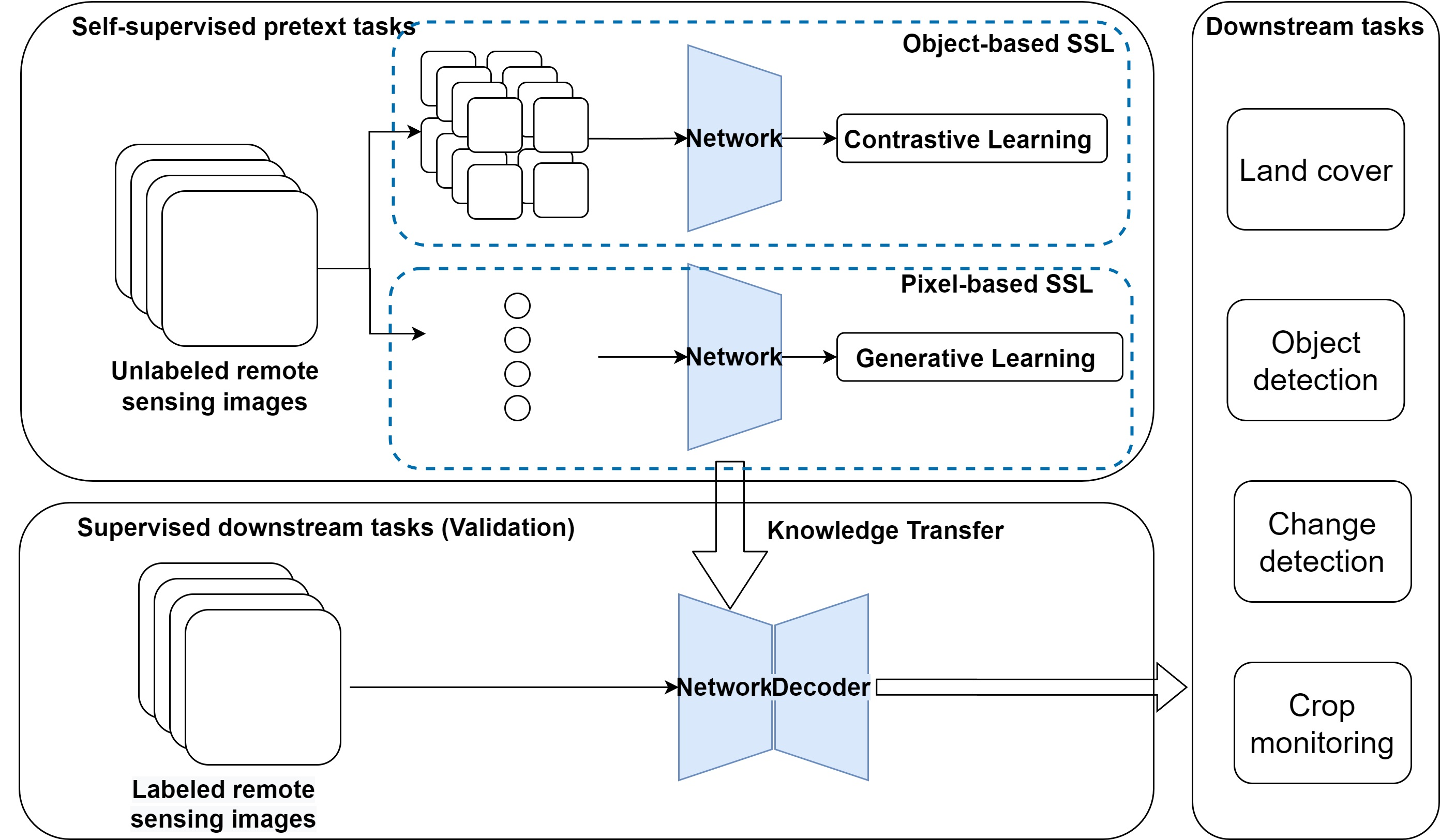
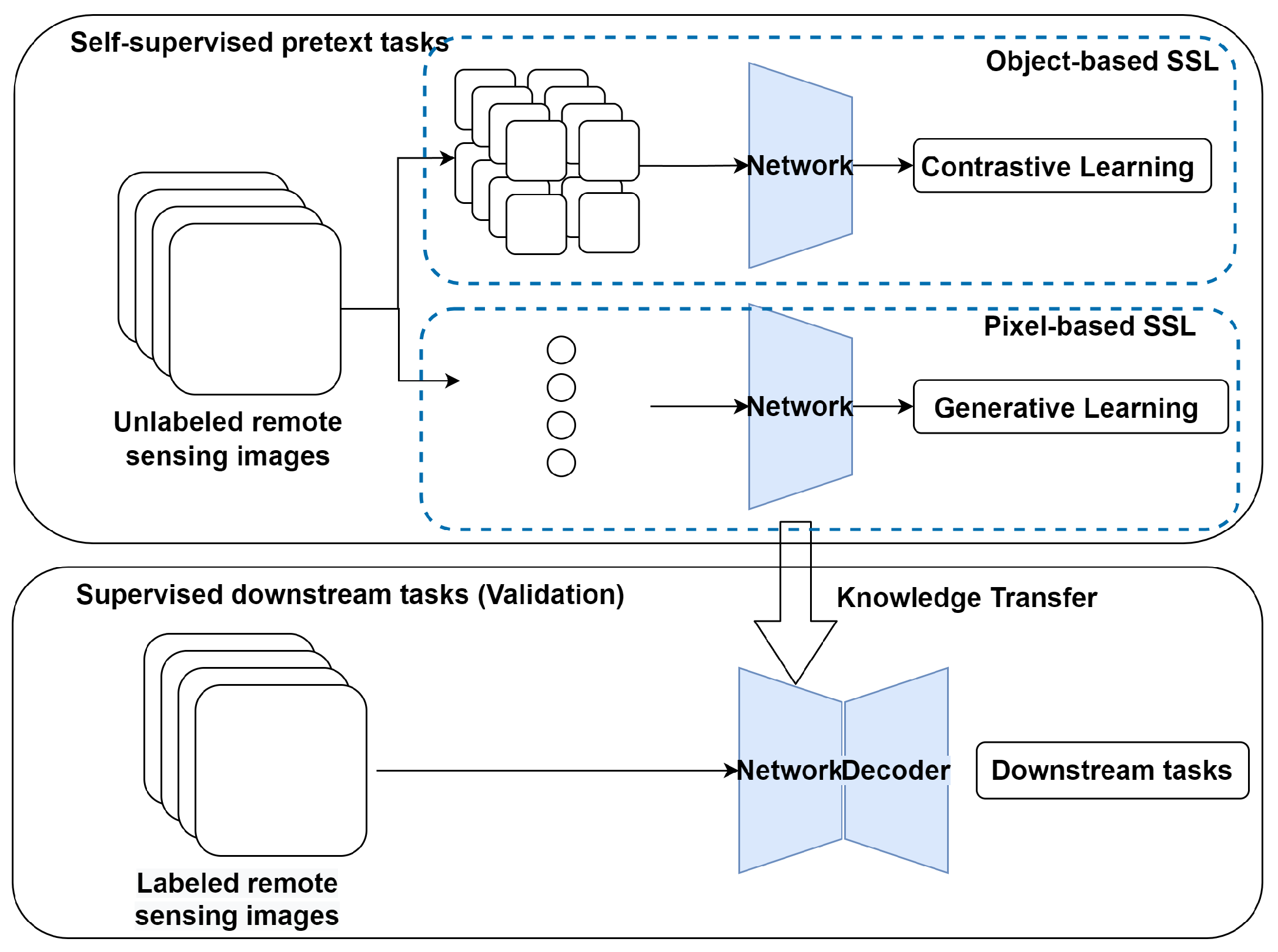
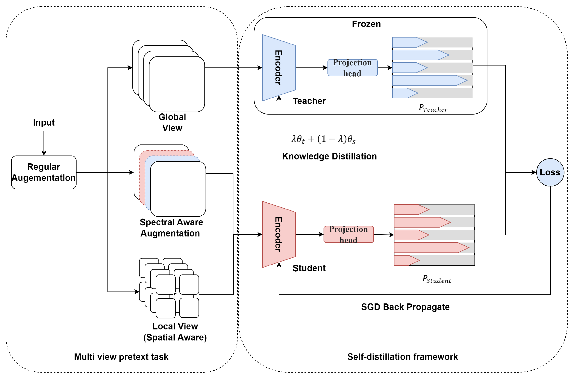
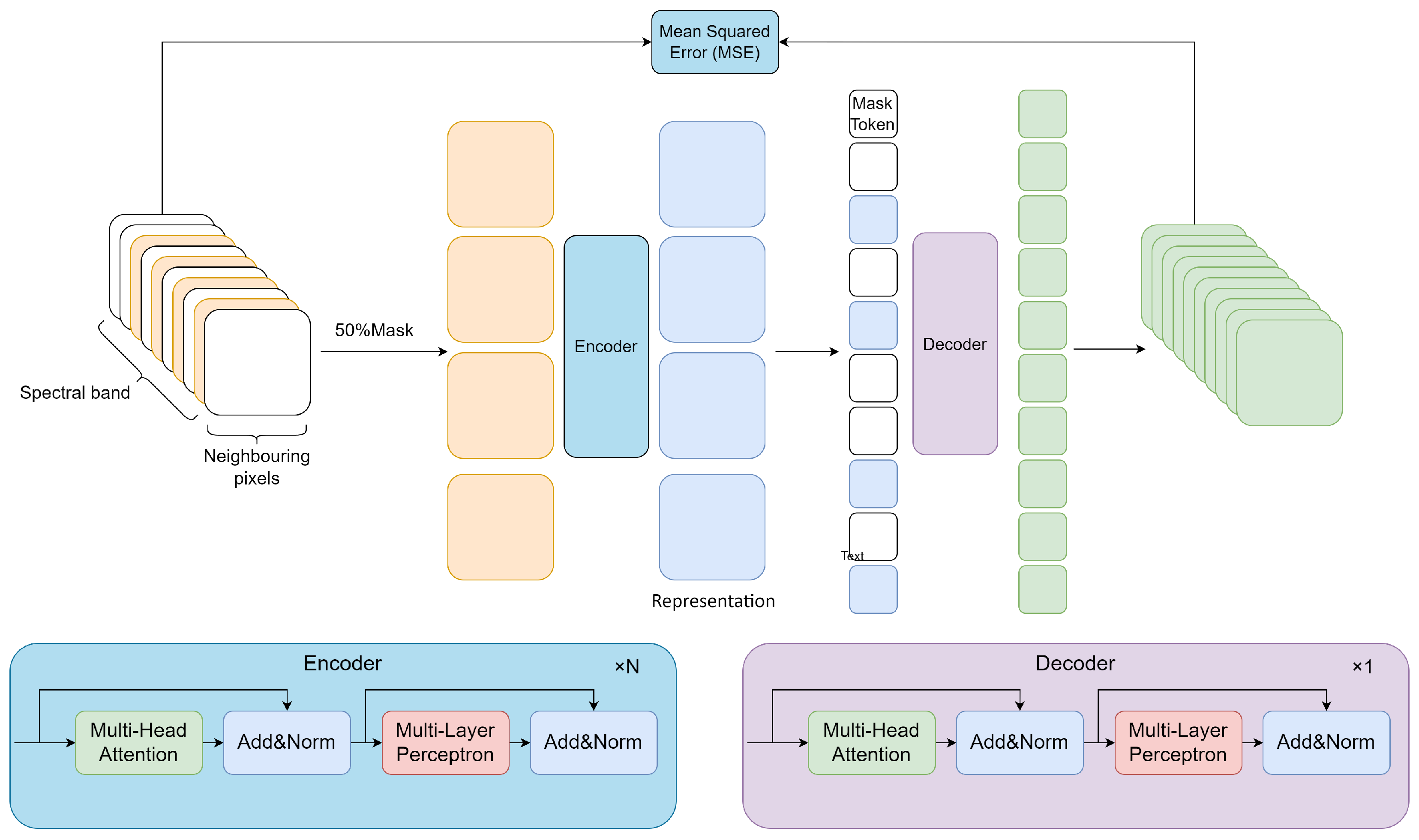
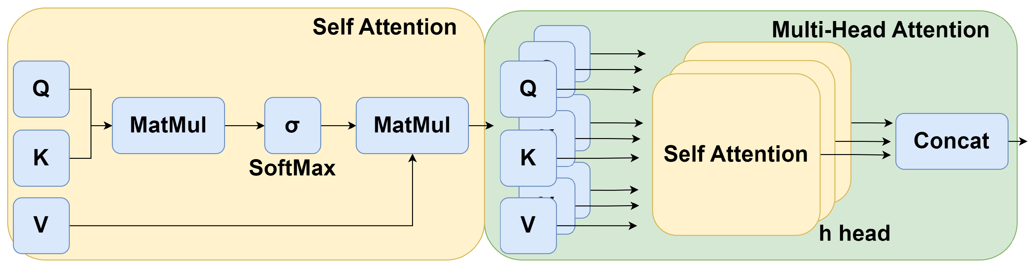
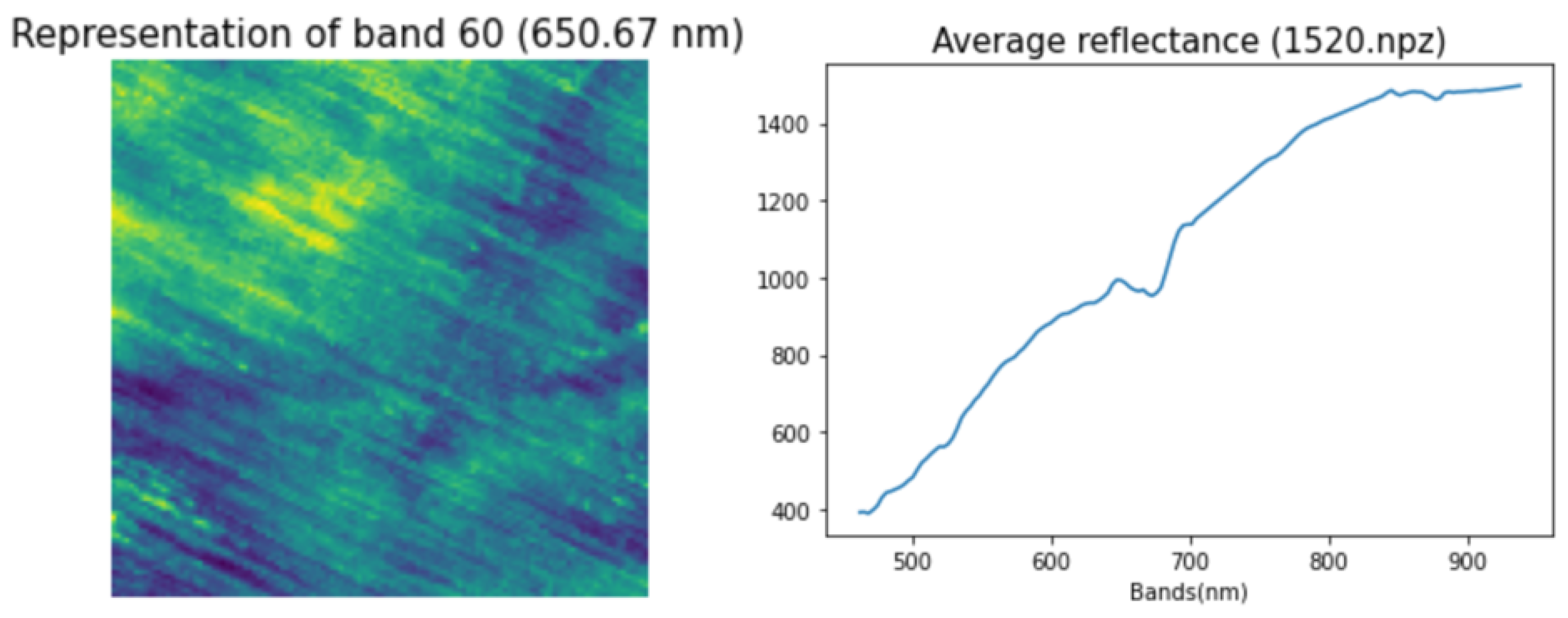
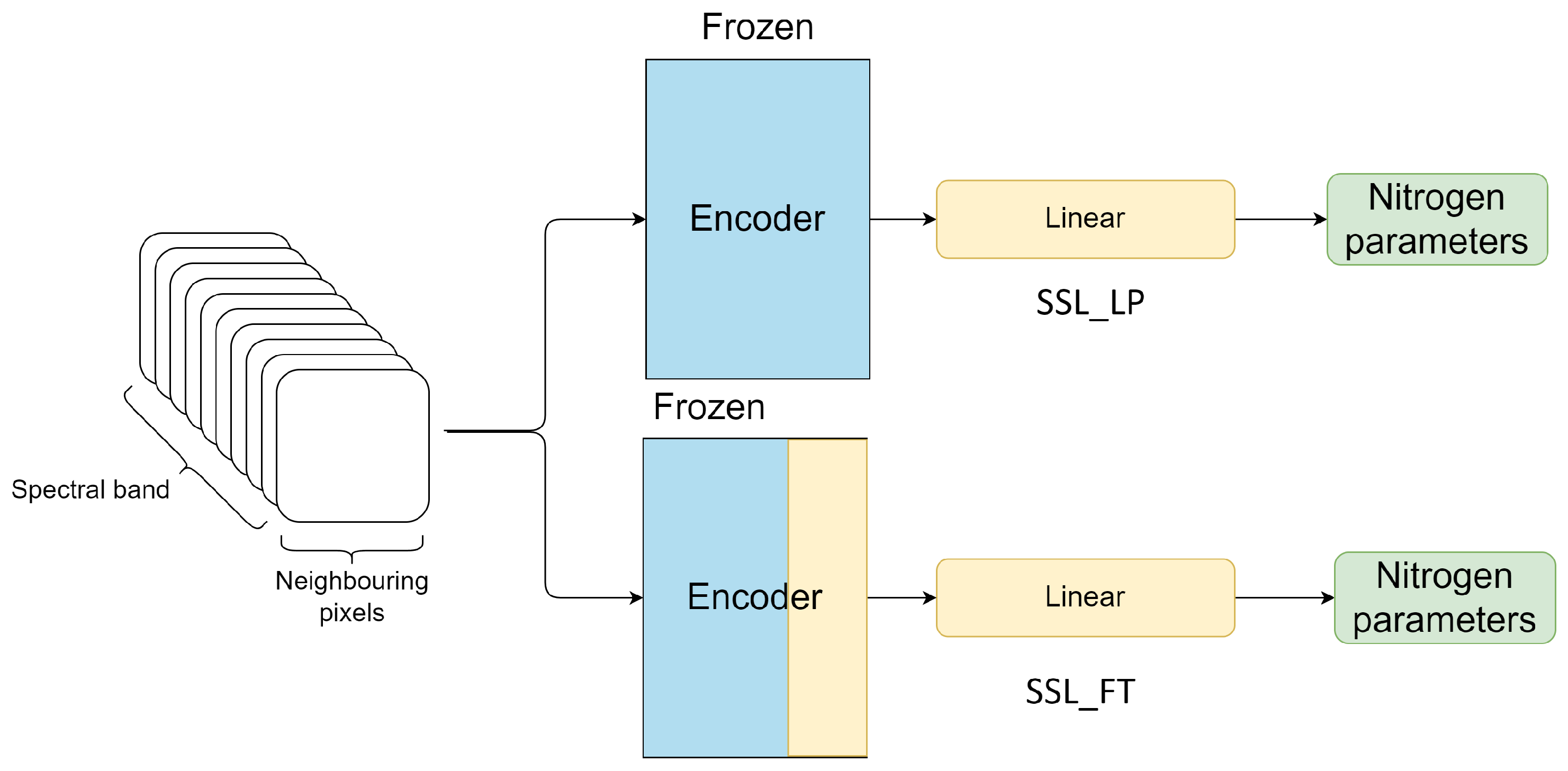
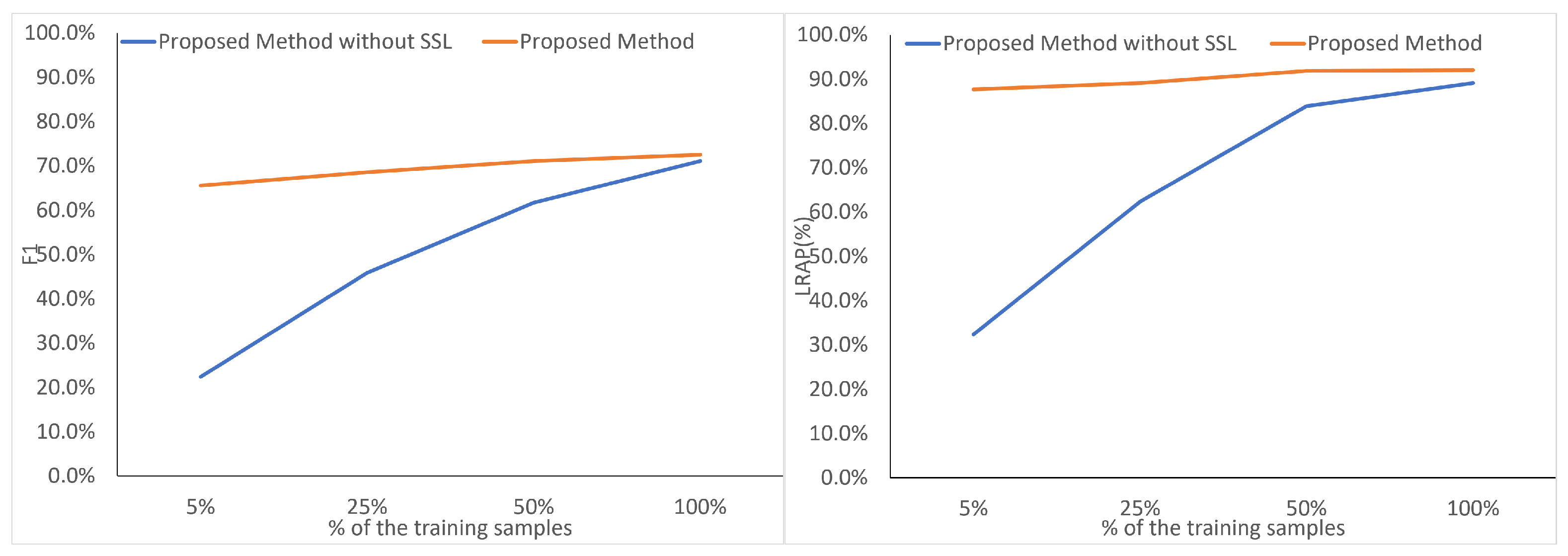
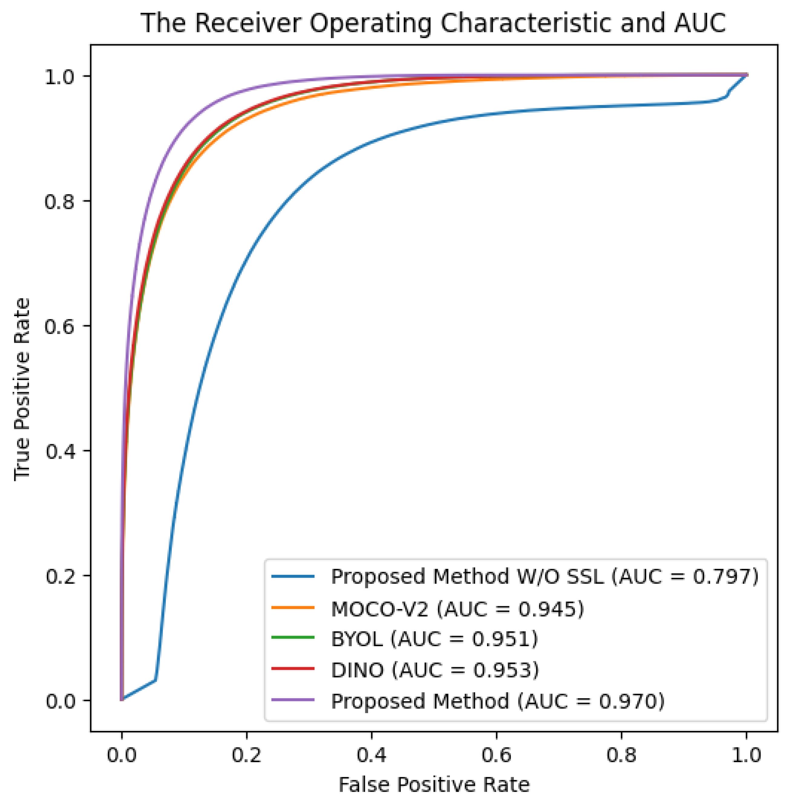
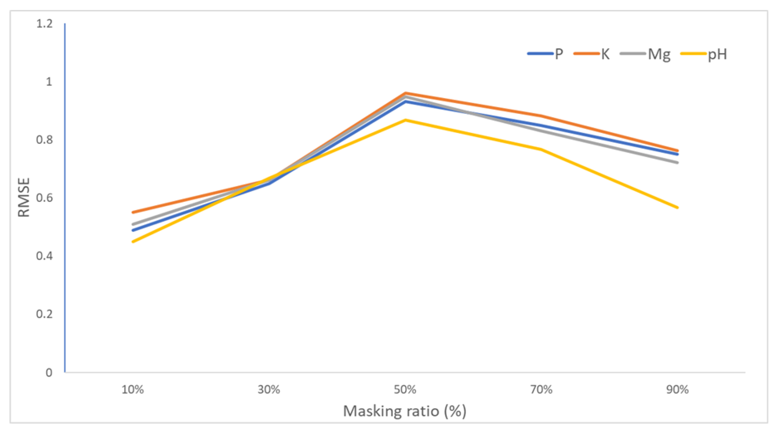
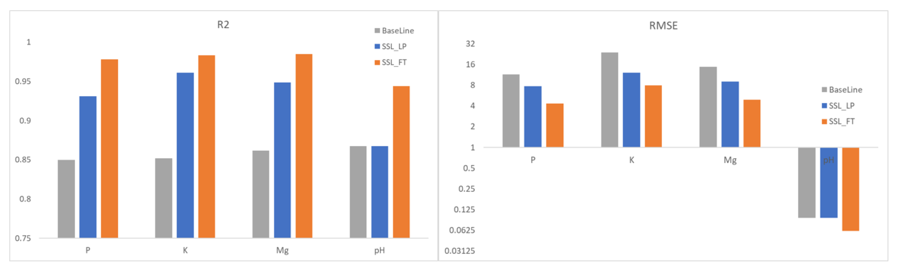
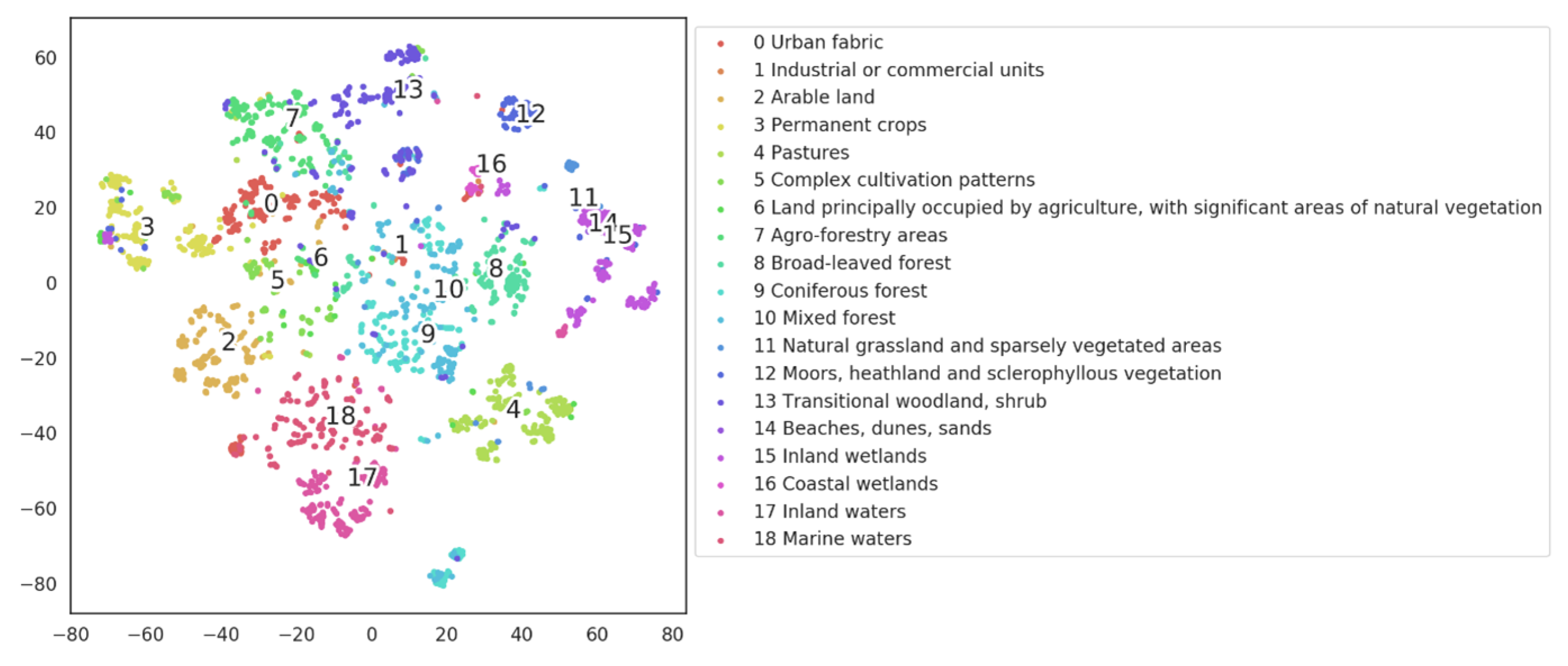
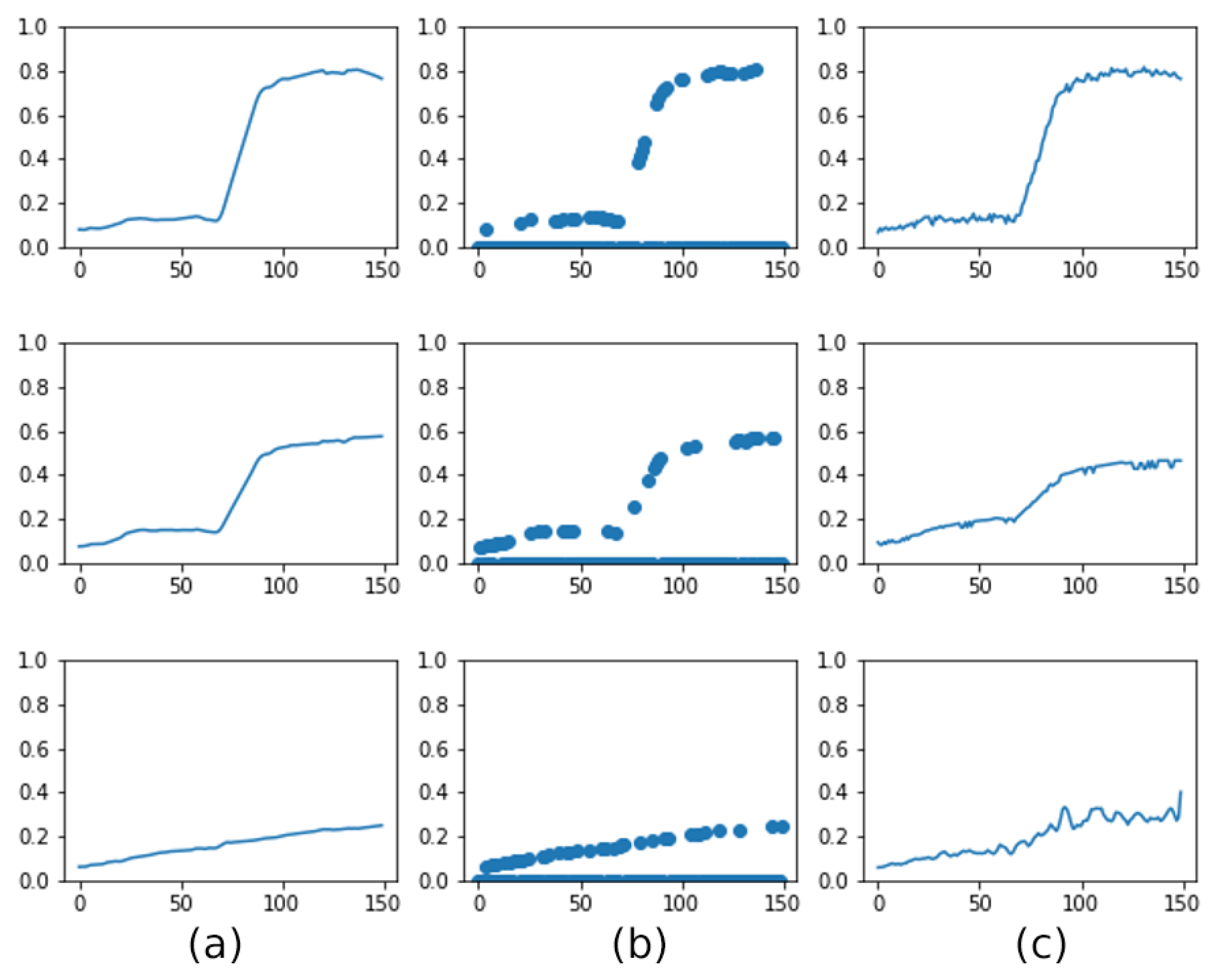
Table 1.
A representative collection of pretext tasks in the existing SSL methods.
| CATEGORY | Name | Pretext Task |
|---|---|---|
| Generative based | Denoising AE [52] | Reconstruct clear image from noisy input |
| Masked AE (MAE) [28] | Reconstruct randomly masked patches | |
| GANs [53] | Adversarial training with a generator and a discriminator | |
| Wasserstein GAN [54] | Train the generator to produce samples that are as close as possible to the real data distribution | |
| Relative position [46] | Predict the relative positions of random patch pairs | |
| Rotation [29] | Predict the rotation angle of a randomly rotated image | |
| puzzle [47] | Predict the correct order of the puzzle | |
| Contrastive learning based | MoCo V1-V3 [55,56,57] | Store negative samples in a queue and perform momentum updates to the key code. |
| SwAV [50] | Contrastive learning for online clustering | |
| BYOL [51] | Average a teacher network with a predictor on top of a teacher encoder | |
| SimSiam [58] | Explore the simplest contrasting SSL designs |
Table 2.
Number of images of each class.
| Class Nomenclature | Training | Validation |
|---|---|---|
| Urban fabric | 56,963 | 17,928 |
| Industrial or commercial units | 9057 | 2808 |
| Arable land | 146,998 | 47,150 |
| Permanent crops | 22,538 | 6812 |
| Pastures | 74,827 | 24,170 |
| Complex cultivation patterns | 78,565 | 25,638 |
| Land principally occupied by agriculture, with significant areas of natural vegetation | 98,585 | 32,052 |
| Agro-forestry areas | 23,388 | 7261 |
| Broad-leaved forest | 107,170 | 34,130 |
| Coniferous forest | 125,243 | 39,532 |
| Mixed forest | 133,926 | 42,641 |
| Natural grassland and sparsely vegetated areas | 9223 | 2799 |
| Moors, heathland and sclerophyllous vegetation | 12,408 | 3859 |
| Transitional woodland, shrub | 112,739 | 36,211 |
| Beaches, dunes, sands | 1315 | 221 |
| Inland wetlands | 16,751 | 5349 |
| Coastal wetlands | 1256 | 310 |
| Inland waters | 51,100 | 16,177 |
| Marine waters | 56,854 | 18,023 |
| Total number of images | 393,418 | 125,866 |
Table 3.
Class-based performance obtained without and with spectral-aware and LaG augmentation.
| W/o Spectral-Aware and LaG | W/o Spectral-Aware | Full Augmentations | |||||||
|---|---|---|---|---|---|---|---|---|---|
| Precision | Recall | f1-Score | Precision | Recall | F1-Score | Precision | Recall | F1-Score | |
| Urban fabric | 72.84% | 60.08% | 65.84% | 72.22% | 65.94% | 68.94% | 86.51% | 71.45% | 78.26% |
| Industrial or commercial units | 59.18% | 28.49% | 38.46% | 62.34% | 39.79% | 48.58% | 83.62% | 25.39% | 38.95% |
| Mixed forest | 78.08% | 79.01% | 78.54% | 82.70% | 78.78% | 80.69% | 85.07% | 82.13% | 83.58% |
| Natural grassland and sparsely vegetated areas | 50.68% | 30.55% | 38.12% | 61.50% | 36.45% | 45.77% | 70.54% | 43.59% | 53.89% |
| Moors, heathland and sclerophyllous vegetation | 58.85% | 41.54% | 48.70% | 71.74% | 46.30% | 56.28% | 73.12% | 61.06% | 66.55% |
| Transitional woodland, shrub | 60.65% | 57.01% | 58.77% | 66.53% | 61.36% | 63.84% | 69.19% | 66.93% | 68.04% |
| Beaches, dunes, sands | 29.25% | 36.44% | 32.45% | 41.43% | 49.15% | 44.96% | 59.72% | 36.44% | 45.26% |
| Inland wetlands | 64.18% | 42.92% | 51.44% | 69.05% | 55.14% | 61.31% | 79.48% | 53.54% | 63.98% |
| Coastal wetlands | 29.63% | 25.57% | 27.45% | 37.19% | 68.95% | 48.32% | 53.70% | 63.01% | 57.98% |
| Inland waters | 83.82% | 79.84% | 81.78% | 88.81% | 79.38% | 83.83% | 90.86% | 80.05% | 85.11% |
| Marine waters | 97.11% | 97.08% | 97.09% | 97.43% | 97.77% | 97.60% | 98.25% | 98.06% | 98.15% |
| Arable land | 83.14% | 79.47% | 81.26% | 82.88% | 83.74% | 83.31% | 89.03% | 83.66% | 86.26% |
| Permanent crops | 53.15% | 43.80% | 48.02% | 71.97% | 38.42% | 50.10% | 73.92% | 60.07% | 66.28% |
| Pastures | 72.48% | 65.55% | 68.85% | 84.83% | 60.43% | 70.58% | 83.39% | 69.27% | 75.67% |
| Complex cultivation patterns | 63.51% | 56.90% | 60.02% | 73.53% | 57.26% | 64.38% | 74.89% | 66.78% | 70.60% |
| Land principally occupied by agriculture, with significant areas of natural vegetation | 61.57% | 56.41% | 58.88% | 75.10% | 46.42% | 57.37% | 71.97% | 63.75% | 67.61% |
| Agro-forestry areas | 69.91% | 66.53% | 68.18% | 79.29% | 65.04% | 71.46% | 79.59% | 78.61% | 79.10% |
| Broad-leaved forest | 74.24% | 68.35% | 71.17% | 84.70% | 62.51% | 71.93% | 81.69% | 76.61% | 79.07% |
| Coniferous forest | 83.75% | 82.77% | 83.26% | 84.04% | 87.48% | 85.73% | 90.03% | 83.45% | 86.62% |
| Average Score | 65.58% | 57.80% | 60.96% | 73.02% | 62.12% | 66.05% | 78.66% | 66.52% | 71.10% |
Table 4.
Results obtained by MOCO-V2, BYOL, DINO, and the proposed SSL pre-trained and fine-tuned on 50% of the training data.
Table 4.
Results obtained by MOCO-V2, BYOL, DINO, and the proposed SSL pre-trained and fine-tuned on 50% of the training data.
| MOCO-V2 | BYOL | DINO | Proposed Method | |
|---|---|---|---|---|
| Accuracy(%) | 91.71% | 91.86% | 92.05% | 92.76% |
| Precision(%) | 65.58% | 70.62% | 69.42% | 73.02% |
| Recall(%) | 57.80% | 50.68% | 55.21% | 62.12% |
| F1(%) | 60.96% | 57.03% | 60.65% | 66.05% |
| HL | 0.083 | 0.081 | 0.080 | 0.072 |
| COV | 4.781 | 4.645 | 4.601 | 4.241 |
| LRAP(%) | 86.25% | 86.33% | 87.17% | 89.13% |
| RL | 0.054 | 0.051 | 0.049 | 0.038 |
Table 5.
Results obtained by VGG16, ResNet50, ViT, and the proposed method with and without SSL.
| VGG16 | ResNet50 | ViT | Proposed Network w/o SSL | Proposed Network | |
|---|---|---|---|---|---|
| Accuracy (%) | 90.96% | 92.32% | 89.94% | 92.83% | 93.84% |
| Precision (%) | 68.59% | 69.62% | 57.91% | 72.66% | 77.87% |
| Recall (%) | 40.05% | 58.04% | 34.16% | 61.52% | 69.25% |
| F1 (%) | 45.85% | 62.52% | 39.00% | 65.10% | 72.50% |
| HL | 0.090 | 0.077 | 0.101 | 0.071 | 0.062 |
| COV | 4.849 | 4.502 | 5.303 | 4.130 | 3.940 |
| LRAP (%) | 83.88% | 87.67% | 80.15% | 89.91% | 92.07% |
| RL | 0.059 | 0.046 | 0.076 | 0.031 | 0.028 |
Disclaimer/Publisher’s Note: The statements, opinions and data contained in all publications are solely those of the individual author(s) and contributor(s) and not of MDPI and/or the editor(s). MDPI and/or the editor(s) disclaim responsibility for any injury to people or property resulting from any ideas, methods, instructions or products referred to in the content. |
© 2023 by the authors. Licensee MDPI, Basel, Switzerland. This article is an open access article distributed under the terms and conditions of the Creative Commons Attribution (CC BY) license (https://creativecommons.org/licenses/by/4.0/).
Share and Cite
MDPI and ACS Style
Zhang, X.; Han, L. A Generic Self-Supervised Learning (SSL) Framework for Representation Learning from Spectral–Spatial Features of Unlabeled Remote Sensing Imagery. Remote Sens. 2023, 15, 5238. https://doi.org/10.3390/rs15215238
AMA Style
Zhang X, Han L. A Generic Self-Supervised Learning (SSL) Framework for Representation Learning from Spectral–Spatial Features of Unlabeled Remote Sensing Imagery. Remote Sensing. 2023; 15(21):5238. https://doi.org/10.3390/rs15215238
Chicago/Turabian StyleZhang, Xin, and Liangxiu Han. 2023. "A Generic Self-Supervised Learning (SSL) Framework for Representation Learning from Spectral–Spatial Features of Unlabeled Remote Sensing Imagery" Remote Sensing 15, no. 21: 5238. https://doi.org/10.3390/rs15215238
Note that from the first issue of 2016, this journal uses article numbers instead of page numbers. See further details here.