
Chaotic Properties of Gravity Waves during Typhoons Observed by HFSWR

School of Information Science and Engineering, Harbin Institute of Technology at Weihai, Weihai 264209, China
*
Author to whom correspondence should be addressed.
Remote Sens. 2023, 15(21), 5235; https://doi.org/10.3390/rs15215235
Submission received: 19 September 2023
/
Revised: 28 October 2023
/
Accepted: 1 November 2023
/
Published: 3 November 2023
(This article belongs to the Special Issue Innovative Applications of HF Radar)
Abstract
:The gravity wave produced by typhoons has been an essential subject of study that concerns numerous researchers. The damage to human beings and infrastructure in coastal regions caused by typhoon disasters annually is very severe, and analyzing gravity wave variation is a reliable approach to research typhoons. High-frequency surface wave radar (HFSWR) as an over-the-horizon radar can achieve real-time monitoring of an extensive sea area and space. This paper derived the gravity wave perturbation spectrum by handling high-frequency surface wave radar data during typhoons. The gravity wave spectrum data were examined by applying the chaos examination approaches of the Lyapunov exponent and phase-space reconstruction to the gravity wave spectrum data after processing and extraction. The reconstructed phase space had a specific shape in a certain direction, with the maximum Lyapunov exponent greater than zero. The gravity wave spectrum data are suggested to have chaotic properties through two chaos examination approaches. This paper demonstrated that the gravity waves observed by a radar have chaotic properties through the measurement data of HFSWR. While the chaotic properties suggest that observed gravity wave data are predictable in the short term, they are unpredictable in the long term. Predicting gravity wave data is important for understanding the chaotic properties of the atmosphere and for future gravity wave prediction.
1. Introduction
Gravity waves generated from typhoons allow the transfer of energy to the upper atmosphere, influencing its compositional structure [1,2]. Gravity waves are mediators in electrodynamic and photochemical coupling processes between layers, from the troposphere up to the thermosphere [3,4,5]. Severe global events, such as tsunamis and typhoons, can excite gravity waves in the ionosphere [6,7]. The first systematic explanation of the effect of gravity waves in the ionosphere was presented with a theoretical formulation by Hines, and the propagation and observation of gravity waves in the ionosphere is still being investigated in depth by a number of researchers [8]. Tropical cyclones, as deeply convective systems, are widely regarded as a significant source of gravity waves, whose produced gravity waves with a long wavelength can influence the upper atmosphere to cause traveling perturbations in the ionosphere, i.e., ionospheric traveling perturbations, which are intrinsically a reflection of the neutral atmosphere to the electronic density disturbances induced by gravity waves [9].
The association between the ionosphere and gravity waves is very tight. Song et al. investigated Typhoon Chan-hom (2009) with the Chinese Global Positioning System (GPS) network in combination with an ionospheric sounding instrument. The researchers revealed the existence of mesoscale fluctuations in the observations, which indicated that gravity waves generated by the typhoon were the major cause of the variation in ionospheric fluctuations [9,10]. Additionally, through analysis of data derived from observations during two severe typhoons, Xiao et al. identified significant gravity wave perturbations and concluded that gravity waves are strongly correlated with traveling ionospheric disturbances (TIDs) [11]. The observation of gravity waves caused by intense convective systems, such as typhoons, started in the 1950s; Bauer et al. observed a remarkable increase in ionospheric foF2 (critical frequency of F2 region) during hurricanes with ionosonde [12]. Rice et al. analyzed ionograms acquired from ionospheric measurements located in four distinct regions of Asia, and they suggested that typhoons may be a significant reason for ionospheric perturbations [13]. Huang et al. subsequently investigated the association of typhoons with ionospheric perturbations using statistical analysis and obtained gravity waves through FFT processing detection after data acquisition with high-frequency (HF) radar [10]. Hung et al. analyzed the gravity waves triggered by a typhoon during its passage, as well as the propagation characteristics of gravity waves by means of high-frequency Doppler detector results [14]. Li et al. combined satellite and land-based observation network data to explore gravity waves excited by Typhoon Chaba (2016), which were directly produced by mesospheric gravity waves [15].
Spectral analysis is an effective method for accurately studying the properties of gravity waves as well as their effects [16]. Kim et al. simulated and researched the spectral characteristics of typhoon gravity waves with a three-dimensional mesoscale model and discovered that gravity waves also propagate in other directions of typhoon motion [17]. Wei et al. adopted the two-step FFT approach on meteorological data to acquire the spectral data of gravity waves and researched the characteristics of gravity waves in various altitudes [18]. Furthermore, with decades of development, the high-frequency surface wave radar (HFSWR) not only has the capability of over-the-horizon target detection and remote sensing of sea state, but also achieves effective observation of space weather within the observation range. Lyu et al. proved that HFSWR enabled the observation of gravity waves after processing radar data acquired during Typhoon Rumbia [19]. Additionally, Bristow et al. processed ionospheric reflection data from HF radar to acquire gravity wave power data for a period of time [20]. Understanding the properties and characteristics of gravity waves is essential to their study [21,22]. Chen et al. conducted a numerical simulation study of typhoon-excited gravity waves and analyzed the spectral structure of gravity waves, finding that the gravity waves had a significant single-peaked shape [23].
Chaos theories are extensively used to research nonlinear systems, such as in radar echo studies. Leung et al. modeled wave echoes with chaos analysis and showed that the wave echoes had a fractal dimension [24]. Field et al. calculated chaotic characteristic quantities, such as Lyapunov exponents, from wave echo data at different frequencies and sea states, which were finally determined to be chaotic [25]. These studies confirmed the ability to identify and investigate chaotic systems through the processing of radar signals. Moreover, Unnikrishnan et al. examined the total electron content (TEC) of midlatitude GPS by employing chaos theory and subsequently compared the chaotic properties of TEC at different latitudes and times [26]. Nowadays, many studies on the properties of gravity waves are at the stage of data observation. The Lyapunov exponential spectrum analysis of coupled equations with gravity waves was performed by Roy et al., which revealed the chaotic characteristics; however, the verification of the practical data has not yet been studied [27].
This paper uses typhoon data obtained by HFSWR to process the gravity wave spectrum data and examine the chaotic properties of the gravity wave spectrum data, which eventually indicated that the gravity wave data derived from handling the actual radar data have chaotic properties. It demonstrates that the gravity waves excited by typhoons are chaotic in terms of practical data, which is essential for the comprehension of atmospheric chaotic properties and future gravity wave prediction.
2. Observation Equipment and Typhoon Path
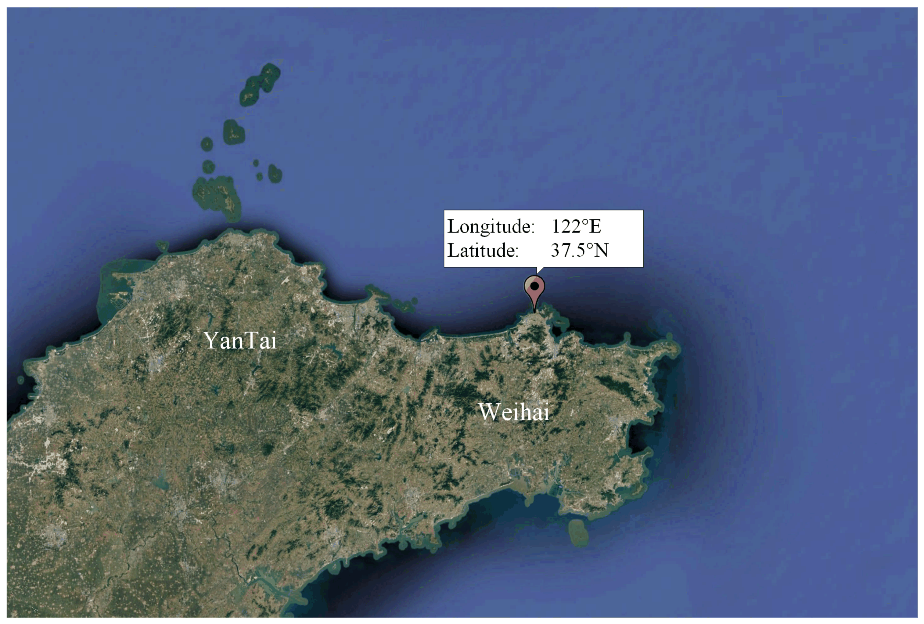
This study utilizes radar data from practical observations of HFSWR in Weihai, Shandong, China, with radar station locations illustrated in Figure 1. The radar operates at frequencies between 3 and 15 MHz, which adopts a pulse truncated linear frequency modulation signal.
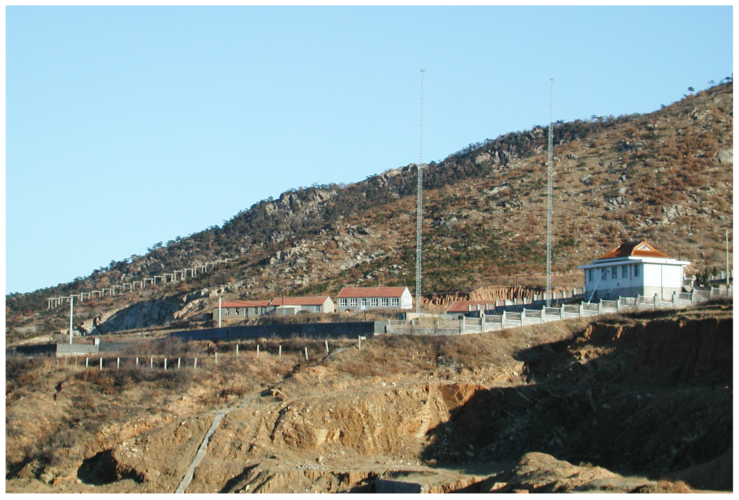
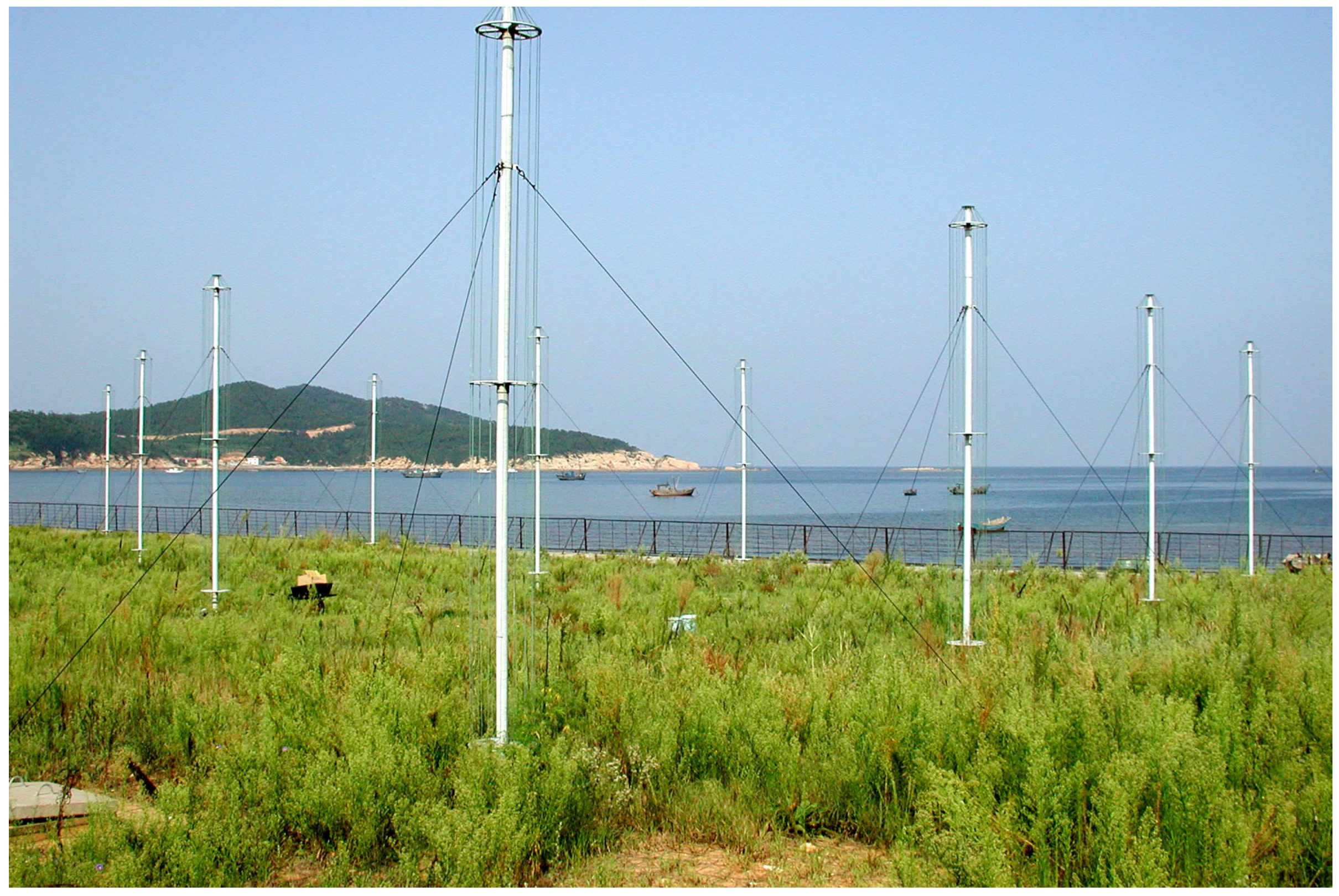
The transmitting antenna is a vertical cage antenna, and the receiving antenna adopts a vertical polarization receiving array of eight-element whip antennas (each array element consists of four antennas) with a transmitting power of 2 kW, which the radar enables to collect the ionospheric echoes from the zenith. The transmitting and receiving antenna arrays of HFSWR are illustrated in Figure 2 and Figure 3.
For the purpose of better research on the detailed variations of the typhoon that passed through the radar observation region, the paper demonstrates the entire trajectory of the typhoon from its generation to its demise. The detailed information is illustrated in the following figure.
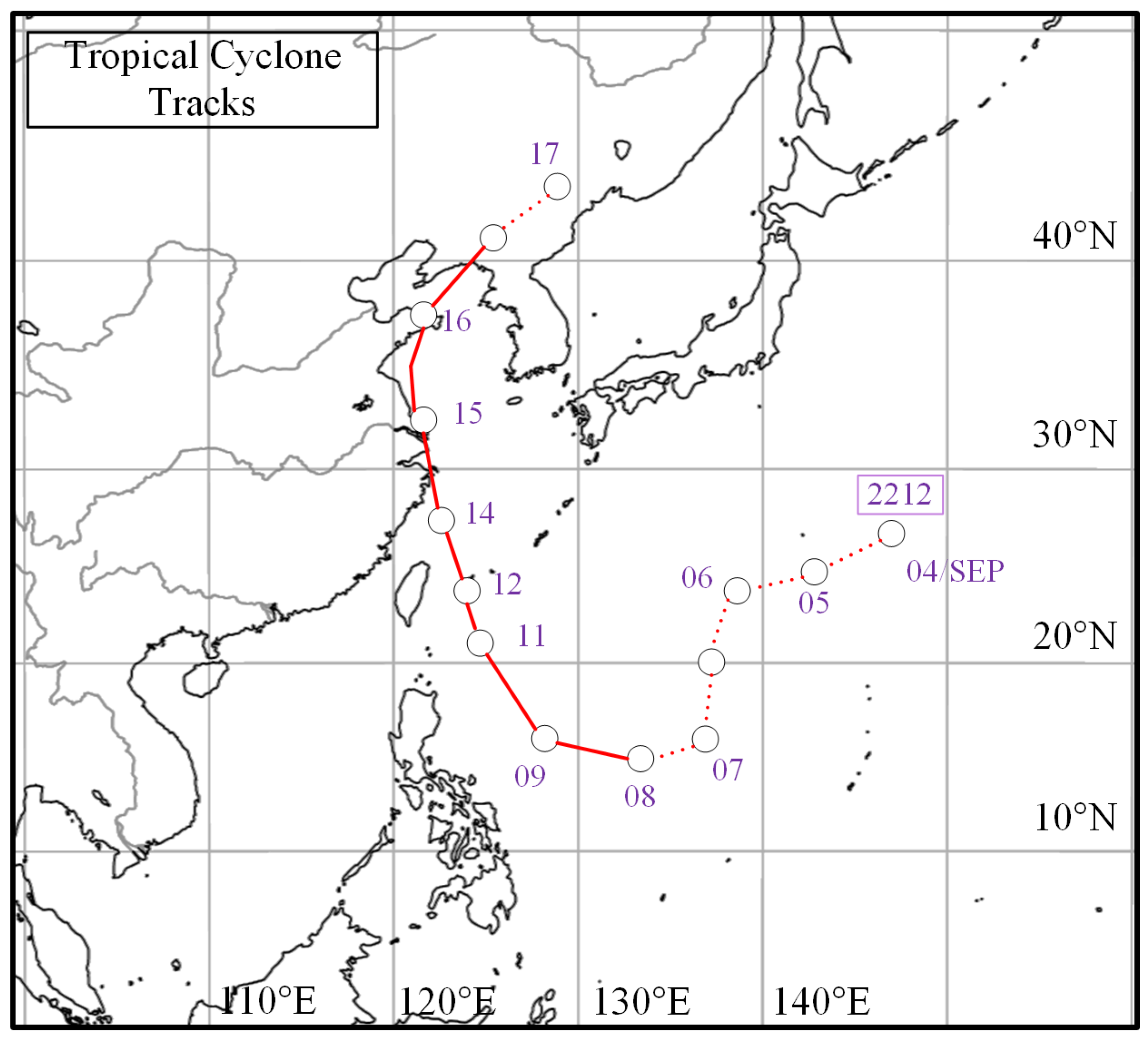
Typhoon Muifa (2022) was generated in the western Pacific Ocean on 4 September 2022, with its path illustrated in Figure 4. The data were obtained from the Japan Meteorological Agency typhoon track data. In Figure 4, the dotted lines indicate the tracks of the typhoon in its developmental and extinction stages. The wind speed of the typhoon reached its maximum on 8 September, the typhoon was in its mature stage, and eventually, the typhoon faded out on 17 September. Therefore, the track of the typhoon from 8 September to 16 September is indicated by the solid line, which represents the movement path of the mature typhoon.
Muifa (2022) was initially a tropical storm, which formed and moved southwestward; then it turned in intensity into a strong tropical storm on 8 September and moved northwestward. On 11 September 2022, at 3:00 LT, the typhoon further developed with the intensity of a strong typhoon, with a maximum wind speed of 50 m and a minimum central pressure of 940 hPa. Subsequently, the typhoon continuously moved northward, which began to enter the sea area of radar observation at 8:00 LT on 16 September 2022. At this time, the strength of the typhoon was a tropical storm with a wind speed of 23 m and a minimum central pressure of 990 hPa. Eventually, the typhoon moved northeast and vanished at 17:00 LT on 16 September 2022. HFSWR in Weihai was operational and collected data throughout the typhoon’s movement through the observation area.
3. Data Processing
The gravity wave data of HFSWR is first extracted from the radar observation data before the gravity wave data are subjected to chaos examination. There are two sections of data processing in this research: the first is data preprocessing, and the other is gravity wave data processing. The specific process is elaborated as follows.
3.1. Data Preprocessing
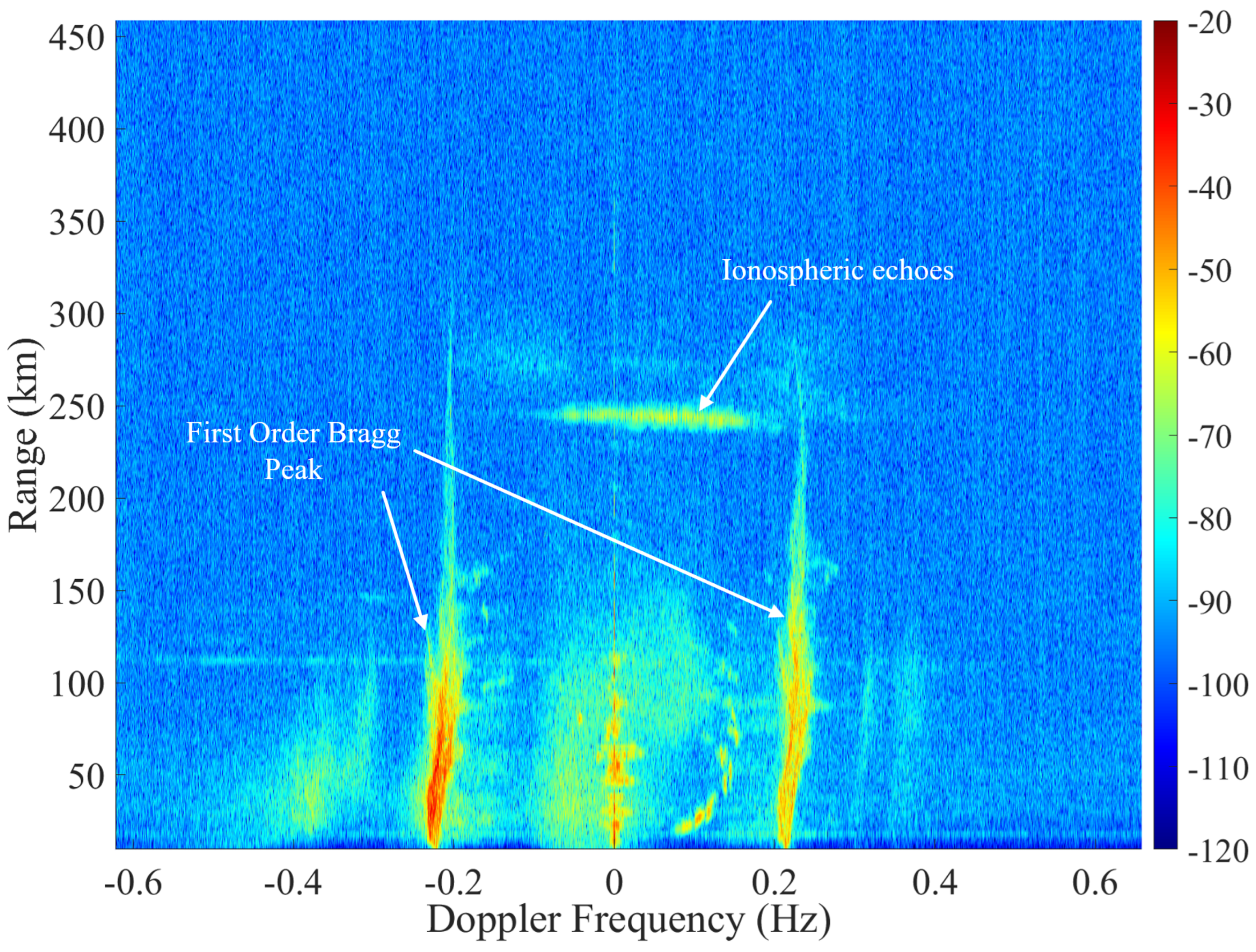
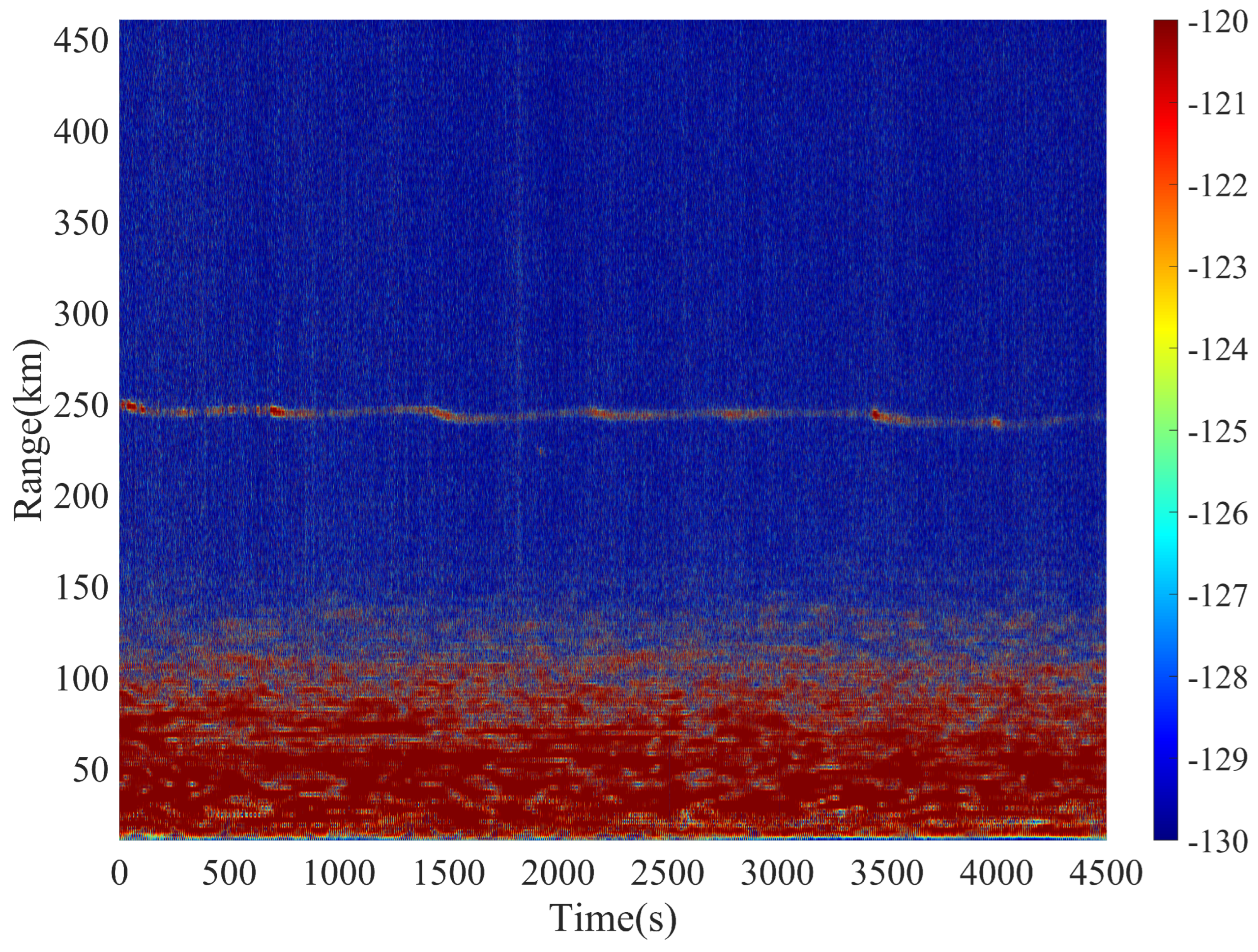
This paper utilizes HFSWR data to process and acquire gravity spectrum data. After the transmitter sends out the signal, the receiver performs analog-to-digital conversion and other operations on the collected signal before the signal processor carries out pulse compression, the matched filtering, and other procedures to eventually derive the range–Doppler spectrum (RD spectrum) within the radar detection range. The typical RD spectrum and distance–time spectrum are shown in Figure 5.
The RD spectrum obtained by processing the radar data by two-step FFT is depicted in Figure 5. The horizontal coordinate indicates the Doppler frequency, while the vertical coordinate denotes the distance. There are two particularly distinct spectral peaks at frequencies around −0.2 Hz and 0.2 Hz, which are the Bragg peaks of the HFSWR ocean echoes. In Figure 5, the transversal spectral peak at 243 km is the ionospheric echo. Furthermore, the points of relatively high signal intensity in the [0, 0.2 Hz] range in Figure 5 are observed vessels, and the spectral peaks at 0 Hz represent ground clutter. The colors in Figure 5 and Figure 6 represent the signal strength in decibels. In the figure, blue represents the weakest signal energy intensity, and red represents the strongest signal energy intensity.
Figure 6 demonstrates the distance spectrum data with only one FFT processing, the horizontal coordinate represents the time, and the vertical coordinate indicates the distance. It is obvious that there is a wave spectrum peak at 243 km, which is the data obtained from ionospheric reflection, and the type of data is the main focus of this study.
3.2. Processing of Gravity Wave Data
This study applies short-time Fourier transform (STFT) processing on the distance spectral data acquired by HFSWR after completing primary FFT processing. The formula related to the short-time Fourier transform is illustrated as follows:
in which is the Fourier transform of , denotes the window function, indicates the signal, represents the time interval, represents the differentiation of the time interval , and f stands for the frequency.
On the basis of the introduction of the paper, it is known that the typhoon generates gravity waves, which can subsequently propagate upward to the height of the ionosphere. During the process of upward propagation of gravity waves, the energy carried by gravity waves can change the electron concentration in the ionosphere. The HFSWR data utilized in the paper not only contain information on the height of the ionosphere, but also include the intensity of the ionospheric echo energy. The intensity information of ionospheric echo energy is derived by the radar based on the reflected echoes of different electron concentrations. Therefore, by processing the ionospheric echo data of HFSWR, it is feasible to acquire data such as the energy of gravity waves and the perturbation period.
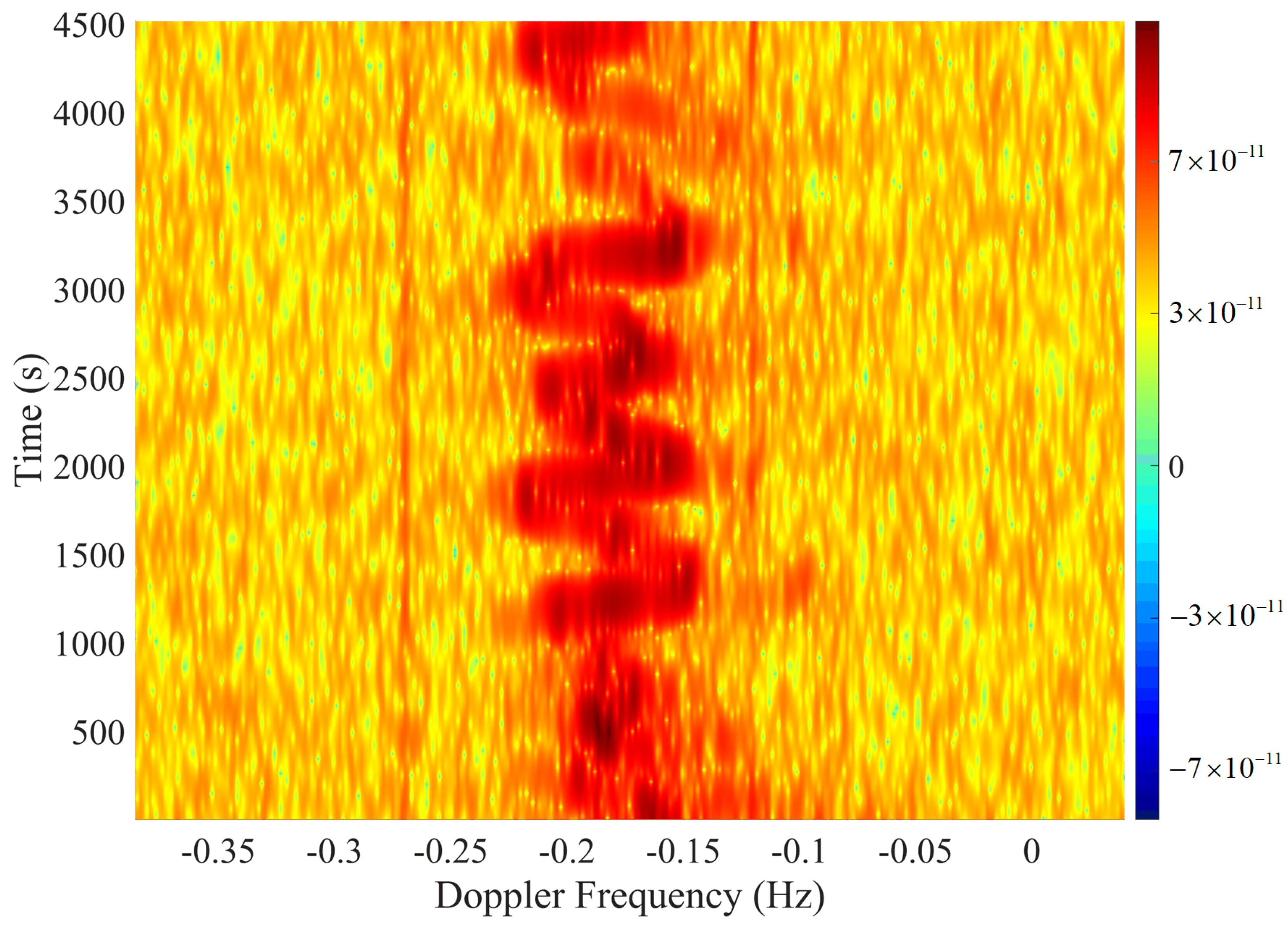
The typhoon came into the radar observation range at 9:00 LT, while it left the radar observation range at 12:00 LT. The data before 9:00 LT were the observation data collected by the radar before the arrival of the typhoon. The ionospheric distance spectrum data of the typhoon crossing with a distance of 243.75 km during the data recording time period of 9:00–10:00 LT were selected before handling; then the short-time Fourier transform was adopted to perform the second step of FFT processing on it, and eventually, the perturbed gravity wave data were obtained. The results of the gravity wave perturbation data are displayed in Figure 7.
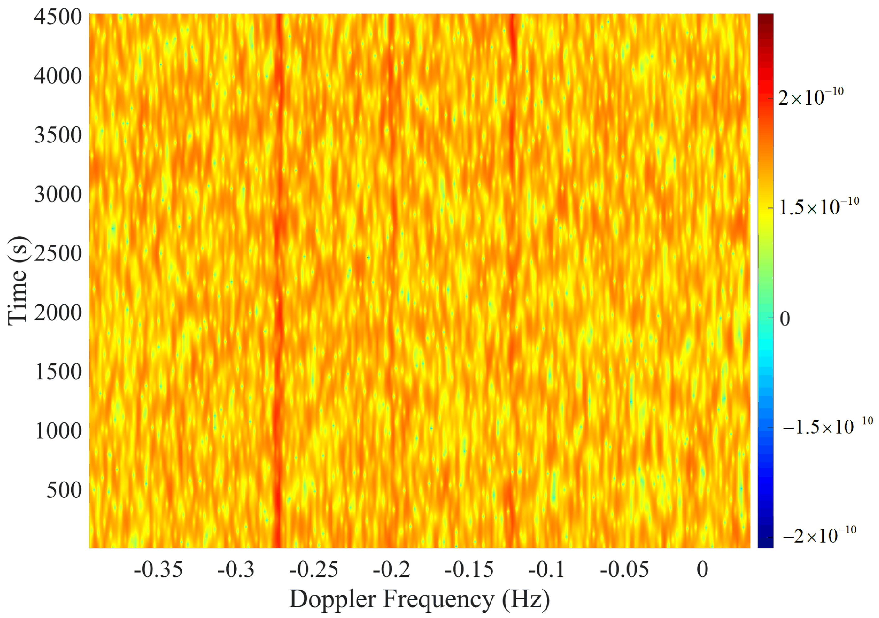
Furthermore, this paper processed STFT on the data at the same distance in the time range of 8:00–9:00 LT before the typhoon. The result of the gravity wave time–frequency spectrum obtained is shown in Figure 8.
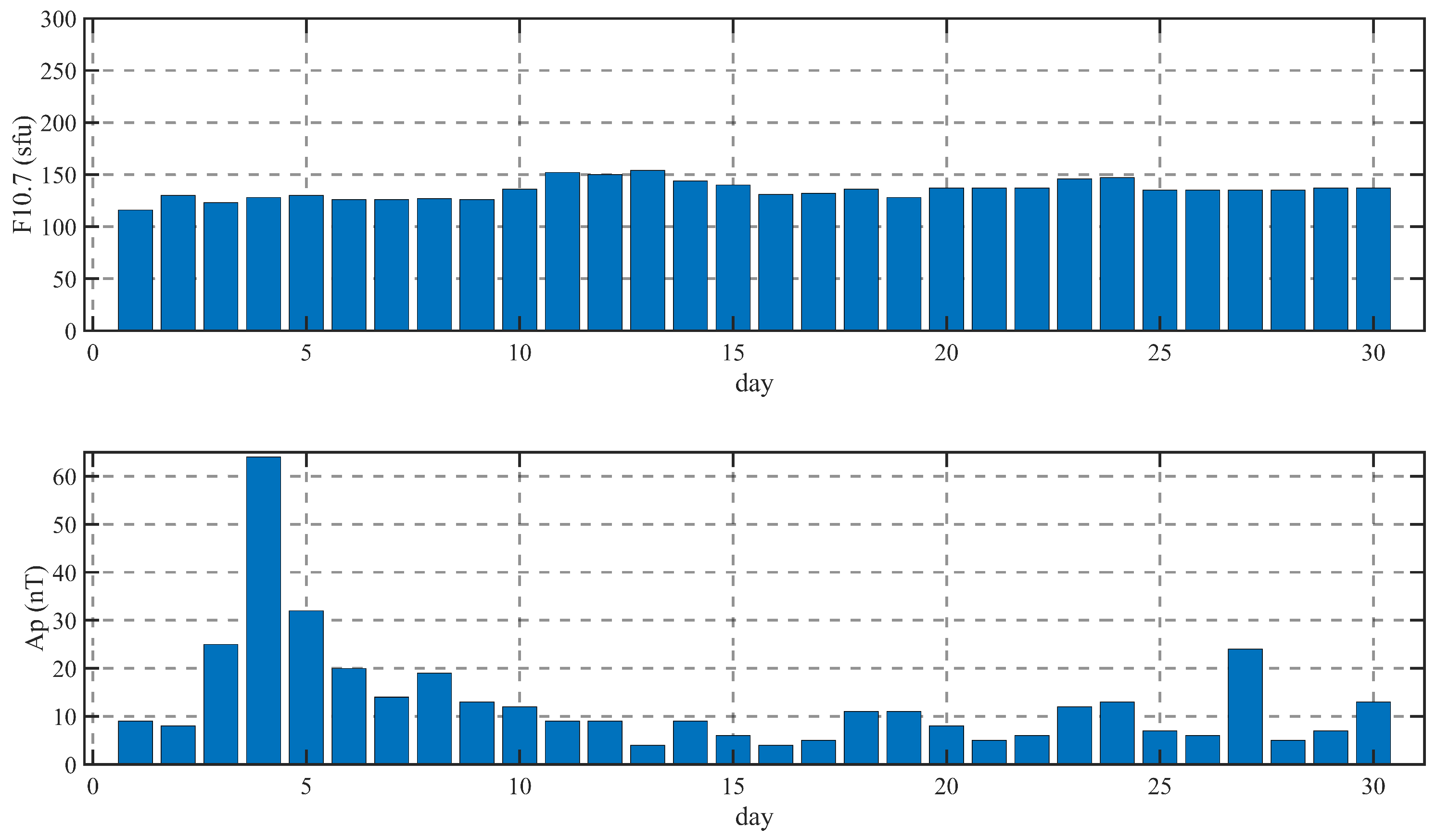
In Figure 7 and Figure 8, the colors in the figures indicate the signal intensity in decibels. The significant gravity wave jitter can be observed in Figure 7, where the gravity wave period is approximately 10 min with the dominant frequency range of the disturbance located between [−0.25 Hz, −0.1 Hz], and the vertical velocity of 10.45 m is derived from the gravity wave period. It is in accordance with the mesoscale perturbation period triggered by tropical cyclones as defined by Dhaka, Bristow, et al. Meanwhile, no apparent gravity wave perturbation is discovered in Figure 8. In addition, the mesoscale gravity wave perturbations are impacted by the solar activity and the geomagnetic surroundings. These two parameters are utilized to describe the intensity of solar activity and the global geomagnetic intensity. The solar radio flux F10.7 data and the geomagnetic AP index (AP index) on the day of data collection and the time period before and after are illustrated in Figure 9, which are sourced from the National Oceanic and Atmospheric Administration (NOAA).
The horizontal coordinate is the 30-day date in September, while the upper vertical coordinate is the F10.7 data in sfu (solar flux unit), and the lower vertical coordinate is the Ap index in nT (nanoteslas). It was evident that the F10.7 data remained at a moderate activity level between 100 and 150 sfu in September 2022, when Typhoon Muifa (2022) arrived, without much variation. The data suggest that the solar activity is relatively stable. In Figure 7, the Ap index is highly variable during the first 10 days of September 2022, indicating strong geomagnetic activity, while the Ap index is consistently low from 11 to 25 September. The Ap index is at the minimum level of 4 on the 16th, which indicates that the geomagnetic activity is stable over this period. These two data illustrate, in another way, that the influence of solar activity and geomagnetic activity on radar observations during radar acquisition of typhoon data is minimal, with the main cause of the perturbed data processed being the gravity waves generated by typhoon excitation.
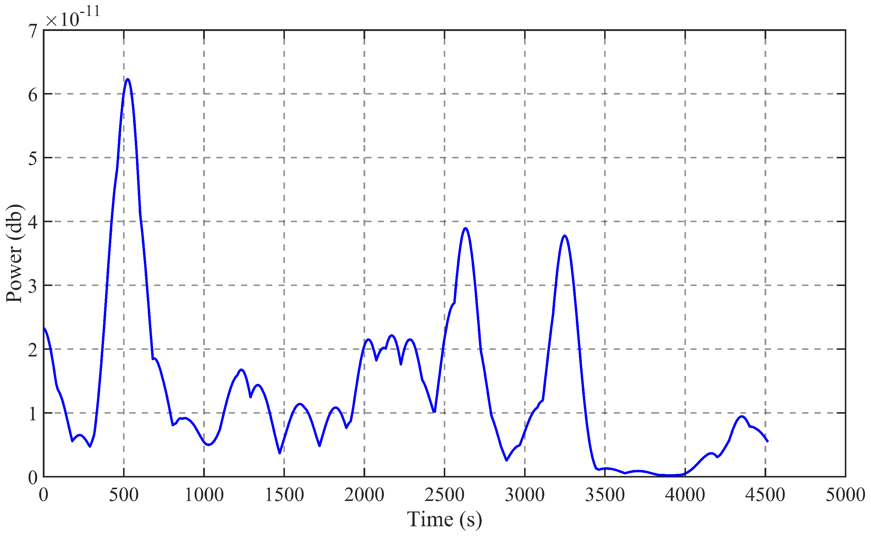
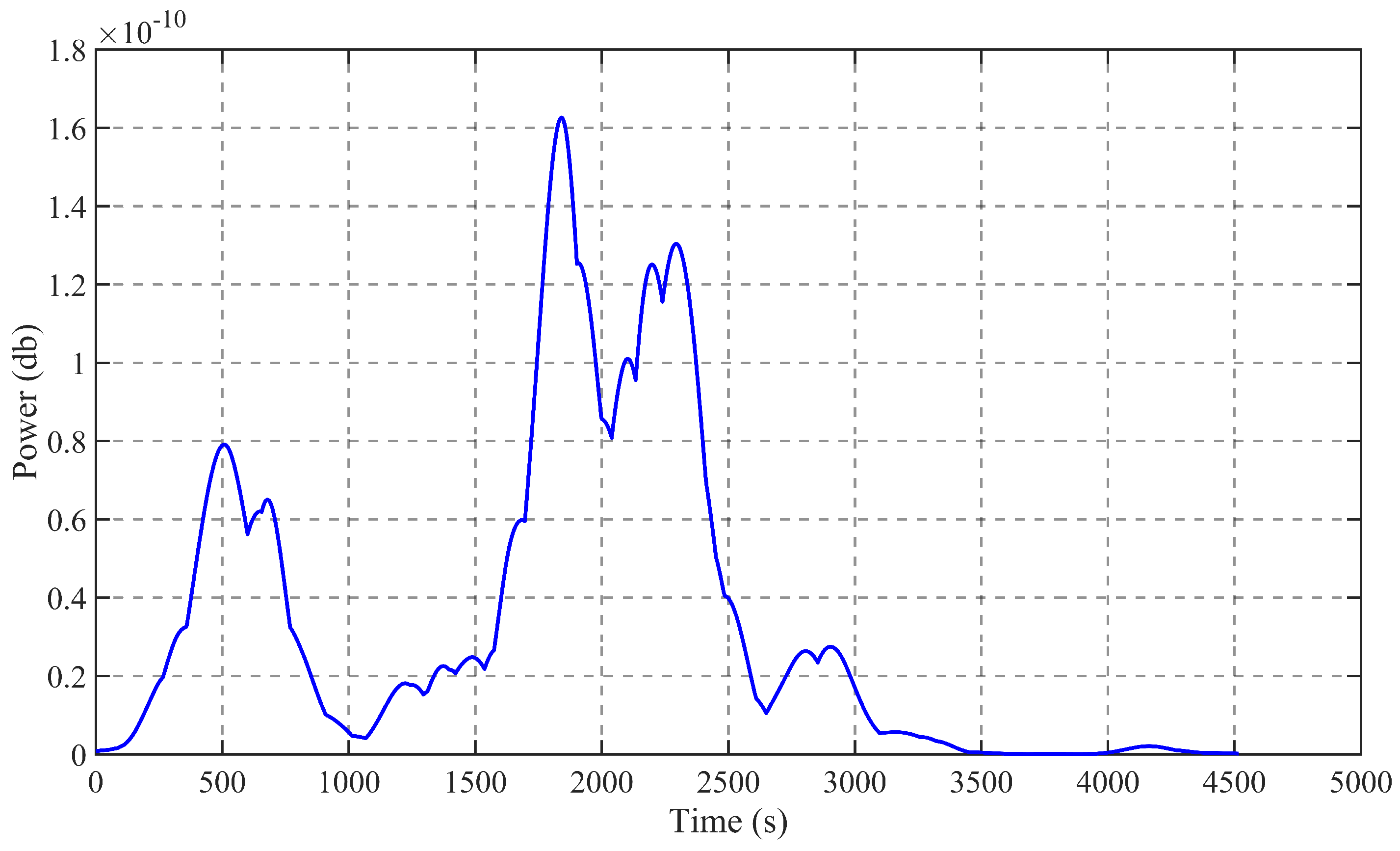
The gravity wave–time spectrum figure acquired from the radar data reveals that the gravity wave data have some diffusion in the perturbation process. The maximum data of gravity spectrum perturbation is extracted in this paper, and in order to avoid interference, the extracted data range is preprocessed to limit the data range to [−0.25 Hz, −0.1 Hz]. The resulting gravity wave perturbed data from the data in Figure 7 and the unperturbed data from Figure 8 are depicted in Figure 10 and Figure 11.
4. Methodology
The chaos is a randomlike phenomenon appearing in deterministic systems, for which intrinsically random solutions derived in deterministic nonlinear systems are named chaotic solutions. Chaotic systems are nonpredictable in the long term; however, short-term processes can be predicted. For chaotic systems, the systematic behavior of the system within the short-term time can be deduced from the initial data [28]. This paper adopts the gravity wave disturbance data derived from typhoon excitation by HFSWR and utilizes the chaotic system analysis approach to determine its chaotic characteristics. The results obtained are of great significance for research on the nature and evolution of typhoon-excited gravity waves. This study determines whether the gravity wave perturbation data are chaotic by the joint phase space reconstruction and Lyapunov exponential spectrum methods, both of which are depicted separately below.
4.1. Phase Space Reconfiguration
The objective of phase space reconstruction is to recover the chaotic attractor by constructing the data into a higher dimensional space, which reveals the regularity of chaotic systems that is an essential feature of chaotic systems. Eventually, the chaotic system displays a specific trajectory, in which the time series is mapped by phase space reconstruction, so that various characteristics of the system can be analyzed. The main steps of phase space reconstruction are as follows:
- (1)
- Calculating the time delay utilizing the de-biased complex autocorrelation method;
- (2)
- Determining the phase space reconstruction embedding dimension with the FNN approach (false nearest neighbor);
- (3)
- Translating the initial time series into a phase space series by using the delay coordinate method;
- (4)
- Constructing the phase space.
In the next step, the FNN method is described. In the geometric perspective, the chaotic time series is a projection of the chaotic motion trajectory of the high-dimensional phase space onto the low-dimensional space, in which the motion trajectory is distorted. It is possible that points that are not adjacent to each other in the phase space of higher dimensions may be adjacent when projected to the lower dimensional space, which is called the false neighbor. Meanwhile, the reconstruction process of phase space is practically finding the primitive chaotic motion trajectories, with the embedding dimension increasing, in which the distorted motion trajectories are gradually decoupled so that the false neighbors are removed. Eventually, the recovered chaotic motion trajectory is acquired, which is the key concept of the FNN approach. The mathematical explanation of it is as follows.
For each vector in the d dimensional phase space, there is a Euclidean nearest neighbor point , where the two vectors are separated by the following distance:
The distance of two points changes as the phase space dimension changes from d to . The new distance is , with the following relation:
If the following relationships are satisfied,
then is regarded as the false nearest neighbor of . Here, represents the threshold value, represents the delay time, and represents its differential. When handling the practical chaotic sequences, the dimension d is incrementally increased, which is regarded as the chaotic attractor being completely opened after the false nearest neighbor points are not growing or the proportion of points are less than 5%, at which time the dimension d is the embedding dimension. The FNN approach is a commonly applied method to calculate the embedding dimension [29,30].
4.2. Lyapunov Exponent
The fundamental characteristic of chaotic systems is the fact that the system is extremely sensitive to initial conditions. Even though the trajectories generated by the initial values are close to each other at the beginning, with time, they can separate exponentially, the Lyapunov exponent being the characteristic quantity that describes the separation rate between the trajectories. The Jacobian method [31,32] is one of the high-precision and robust approaches for solving the Lyapunov exponent of the observation time series, which is also utilized in this study to compute the Lyapunov exponent.
Assuming that the system in space, F is a mapping in the range of , k represents the number of time points, and m represents the spatial dimension, the Jacobian matrix formula of F is as follows:
In the equation, , , C represents the input matrix, and F denotes the matrix of partial derivatives. On the basis of the matrix, is described by the following definition:
where the complex root of is expressed as , , . The ith Lyapunov exponent of the system can be denoted as the below formulation:
in which represents the Lyapunov exponent, with different initial values varying in direction when the separation rate changes, hence creating a spectrum of Lyapunov exponents in the same number and phase space dimensions. The exponents of the above equation are ranked, which eventually leads to a maximum Lyapunov exponent (MLE) formula given below:
The system is chaotic with positive values of MLE. The Lyapunov exponent is a significant indicator of the characteristics of time series, and it indicates the average exponential rate at which the system converges or diverges over the phase space. It is an important criterion to examine whether the time series is chaotic or not.
5. Results and Discussion
In this paper, the gravity wave data derived through HFSWR data processing were examined for chaos, and the examination methods adopted the phase space reconstruction method as described in Section 4 and the Lyapunov exponent methodology. Detailed descriptions of the results obtained by both methods for gravity wave data processing are provided in the following subsections.
5.1. Results of Phase Space Reconstruction
The typhoon gravity wave perturbation data derived from HFSWR were investigated by phase space reconstruction and Lyapunov exponent. The time delay of the gravity wave perturbation data was first calculated with the de-biased complex autocorrelation approach. The equation of the de-biased complex autocorrelation approach is as follows:
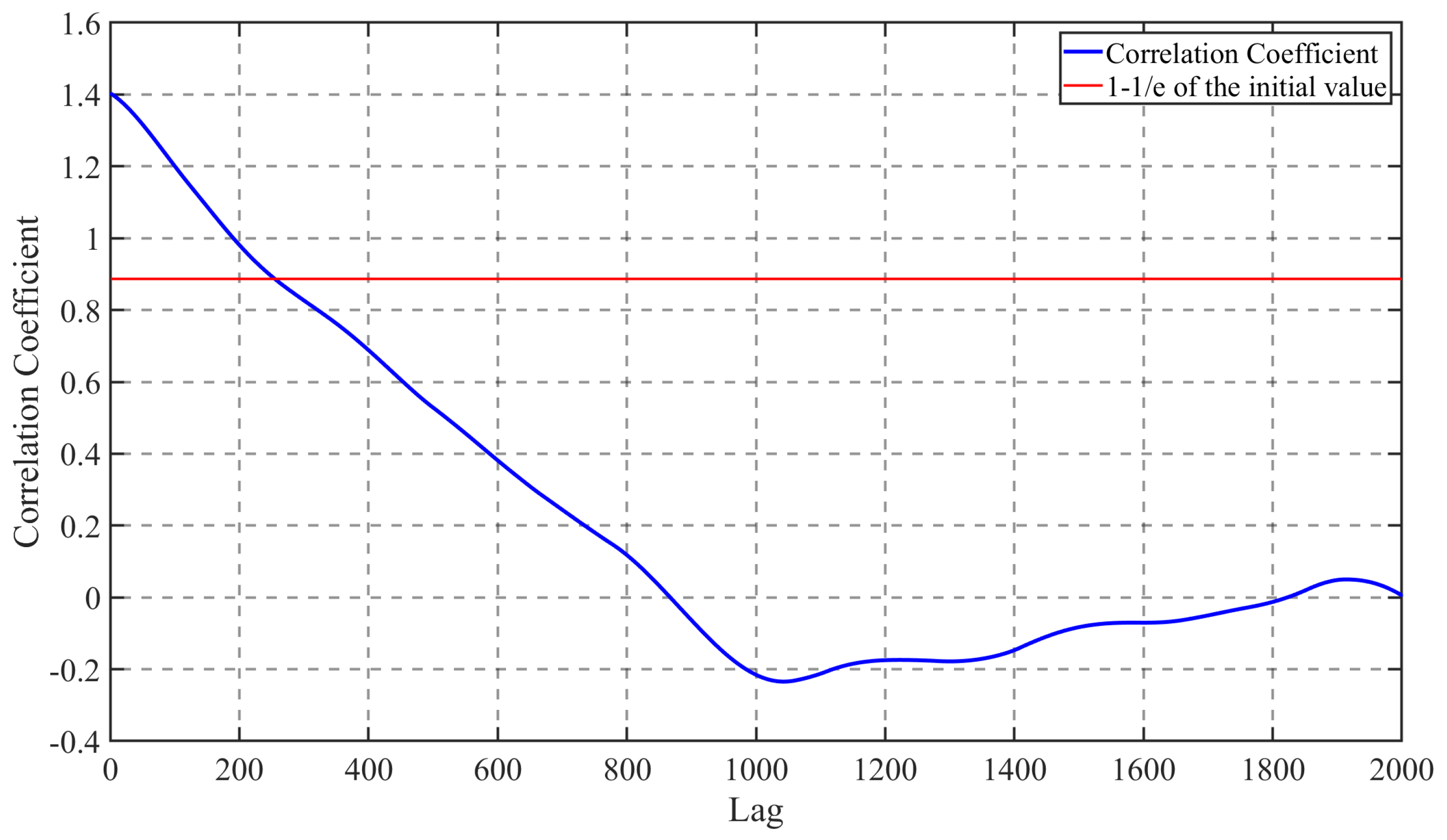
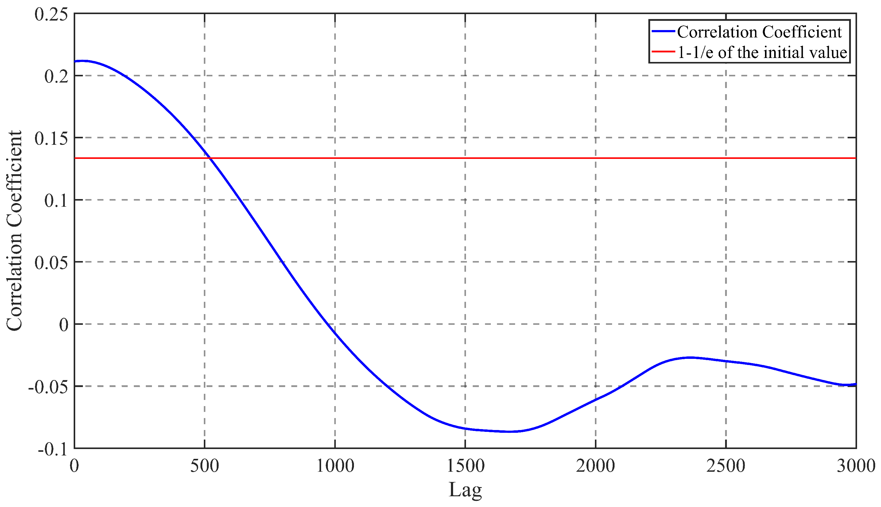
where m stands for the initial dimension, , and is the time delay when the function drops to of the initial value. The function variation pictures of the gravity wave data acquired at two time periods of HFSWR are displayed in Figure 12 and Figure 13.
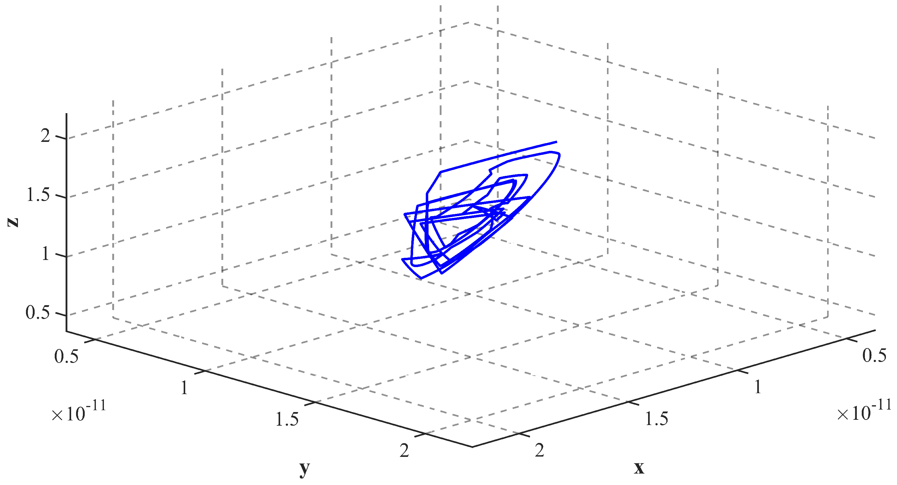
The horizontal coordinate is the lag period and the vertical coordinate is the correlation coefficient. As the function decreases to of the original value, the time delay of the data during the typhoon is calculated to be 255 ultimately, while the time delay of the data before the typhoon is 521. The phase space reconstruction of the gravity wave data is carried out according to the derived time delay and the size of the embedding dimension, and the phase space three-dimensional diagram of the two data after reconstruction is shown as follows.
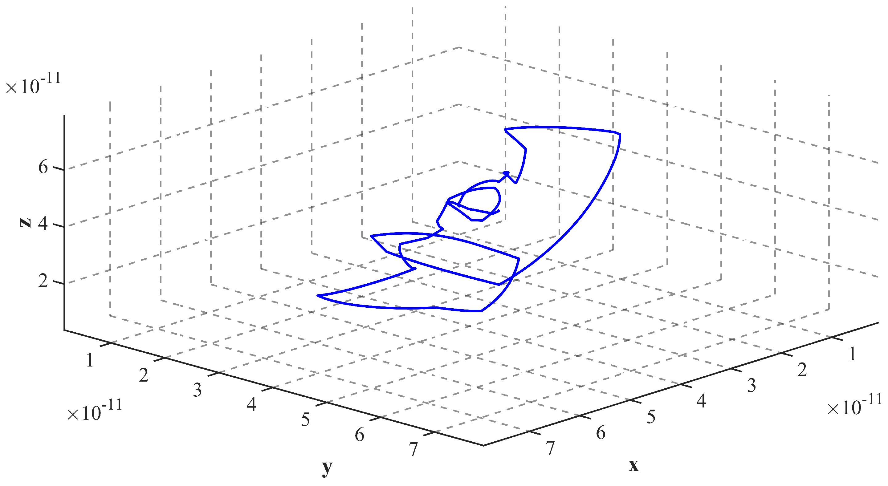
The phase space reconstruction map is a method for distinguishing whether a time series is chaotic or not. The phase space reconstruction map will regularly move around a certain center, and the trajectory has a specific shape when the time series is in a chaotic state, while it does not have this property when the time series is not in a chaotic state. From Figure 14, it can be noticed that the reconstructed phase space attractor has a triangular shape in one direction in space; thus, the result derived from the phase space reconstruction indicates that the gravity wave data have a certain chaotic property. In contrast, Figure 15 indicates an irregular shape and no fixed trajectory, suggesting that the data are not chaotic.
5.2. Results of the Lyapunov Exponent
The time delay and the embedding dimension of the gravity wave time series data were obtained according to the de-biased complex autocorrelation approach and the FNN method. In order to depict the attractor in a more precise way, the Lyapunov exponent was employed in this study to further investigate the characteristic quantities of gravity wave time series over the whole attractor.
This paper adopted the Jacobian approach in which the phase space reconstruction of the gravity wave time series was performed first to calculate the Jacobian matrix of the state equation, followed by the eigenvalue decomposition to derive the Lyapunov exponent. To mitigate the impact of noise on the methodology, the wavelet noise reduction process was applied before the data were subjected to computation. The Lyapunov exponential spectrum of the gravity wave time series was obtained with the Jacobian approach utilizing the already-acquired time delay; the embedding dimension is illustrated below.
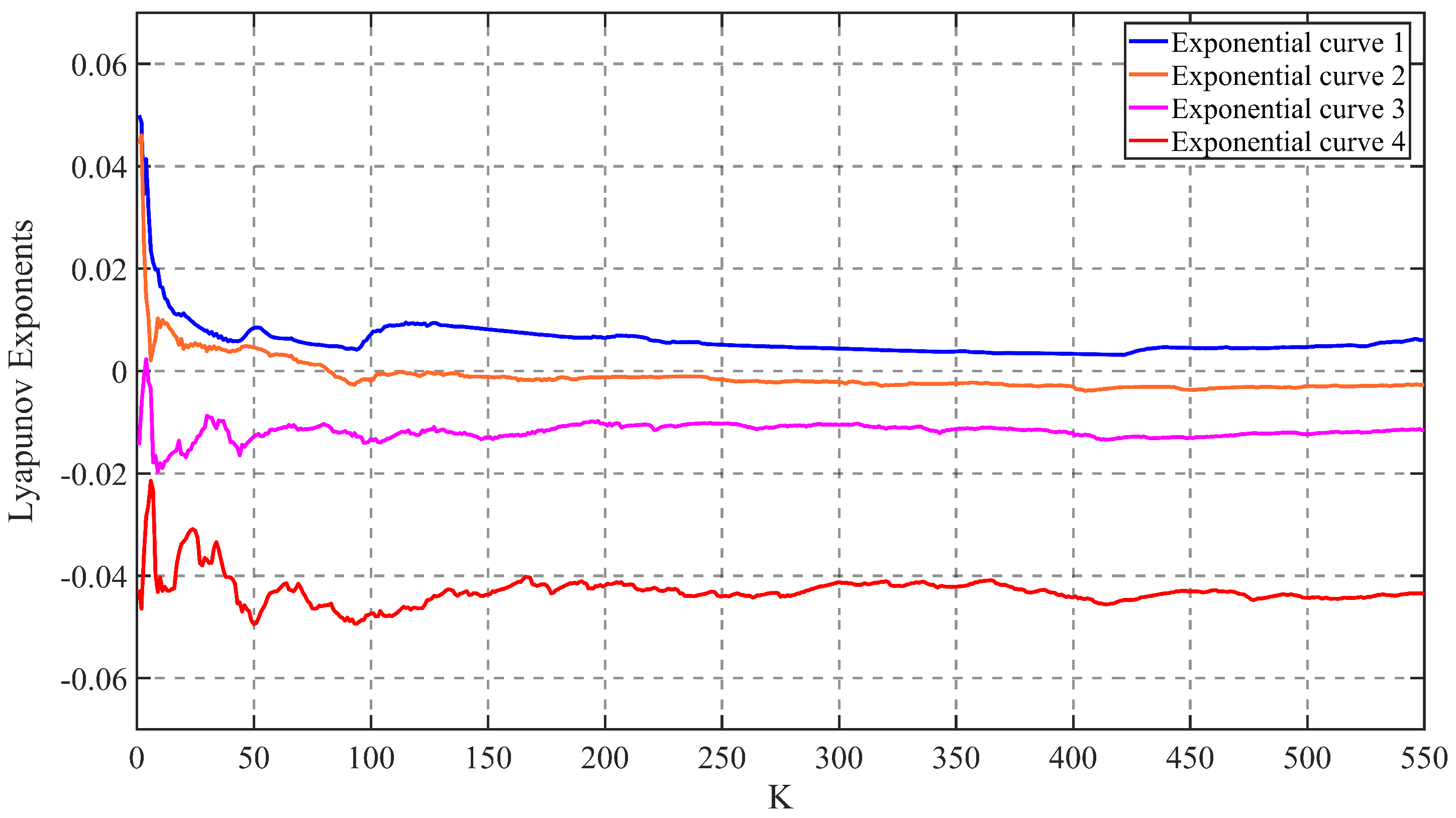
The Lyapunov exponent is an essential parameter applied to determine whether the time series is chaotic or not. The time series is chaotic when the maximum Lyapunov exponent is greater than zero. The vertical coordinate is the Lyapunov exponent, and the horizontal coordinate is the number of iteration steps in Figure 16. The obtained embedding dimension is four, so the data eventually obtain four Lyapunov exponent variation curves. From Figure 16, it is obvious that an exponential change curve is consistently above the value of 0. The maximum and minimum values for each curve in Figure 16 are shown in Table 1.
In Figure 16, whenever one of the curves has a maximum Lyapunov exponent greater than zero, it indicates that the time series is chaotic. Therefore, curves 3 and 4 have no effect on the determination of the chaotic property of the time series, although some data are lower than zero. Furthermore, all of the Lyapunov exponents in curve 1 are greater than zero, suggesting that the chaotic property of the gravity wave data is quite significant. This curve has a maximum Lyapunov exponent value of 0.0499. The results demonstrate that the observationally obtained gravity wave data eventually develop into a chaotic state with time variation, no matter how small the initial distance is in the phase space. This time series is chaotic in character.
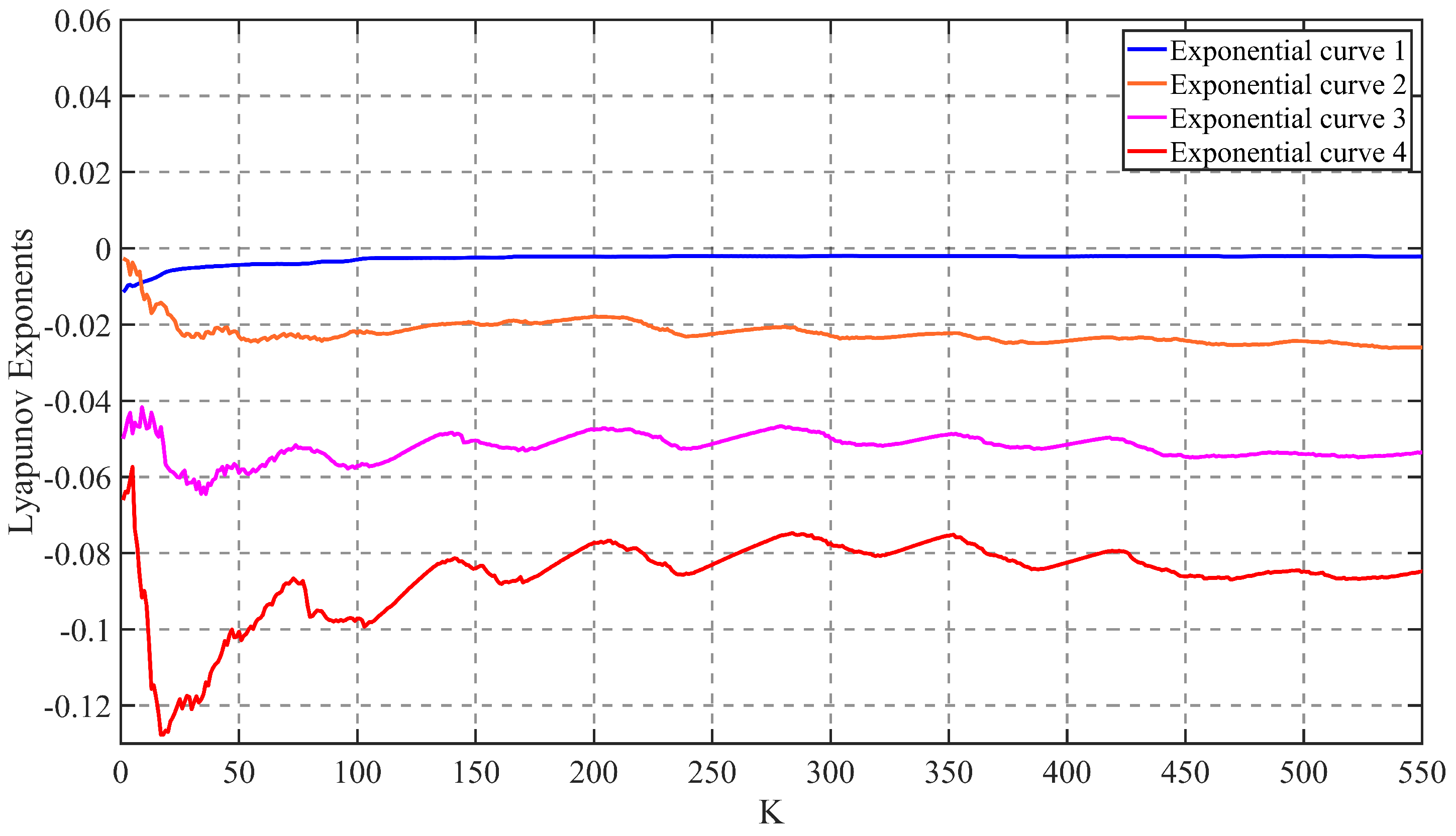
On the contrary, in Figure 17, no exponent in the Lyapunov exponent spectrum is larger than zero for the data collected and processed before the typhoon, and the maximum Lyapunov exponent is −0.0019. Each of the maximum and minimum values of the exponential curves in Figure 17 is shown in Table 2.
From the variation of the Lyapunov exponent spectrum and the maximum Lyapunov exponent, it can be concluded that the gravity waves are not obvious, and the data are not chaotic before the typhoon.
6. Conclusions
In this paper, HFSWR observations during Typhoon Muifa (2022) were acquired, and the gravity wave perturbation spectrograms obtained by two-step FFT processing and the gravity wave disturbance data in the spectrograms were extracted. The solar radio flux F10.7 data and the geomagnetic AP index data recorded on the day of the HFSWR typhoon data collection, and the time periods before and after, suggest that the data were essentially unaffected by solar activity and geomagnetic variations. The data acquired by HFSWR during and before the typhoon were subsequently analyzed for chaotic characteristics with the phase space reconstruction and the Lyapunov exponential method. The gravity wave perturbation data during the typhoon were analyzed to display a triangular shape in the phase space in certain directions and exhibit a specific shape, while the gravity wave was not obvious and had no regular shape in the phase space in the time period before the typhoon.
The gravity wave data acquired during the typhoon were solved for an exponential curve in the Lyapunov exponent spectrum, which was consistently greater than zero, and the maximum Lyapunov exponent was 0.0499, a value greater than zero. In contrast, the gravity wave observation before the typhoon was not significant, and there was no curve larger than zero in the obtained Lyapunov exponent diagram, with a maximum Lyapunov exponent of −0.0019. This finding indicates that the gravity wave does not appear before the typhoon and the data do not have chaotic property. The above two methods of chaotic examination demonstrate the chaotic properties of the gravity wave disturbance data obtained by HFSWR acquisition and processing during the typhoon crossing. The chaotic property implies that the gravity wave time series obtained in this study are predictable in the short term but not in the long term. This result indicates that the gravity wave data acquired in this paper can be investigated for prediction in the short term. This paper verifies the chaotic properties of typhoon gravity waves from the measured data, which is essential for understanding the atmospheric chaotic properties and future gravity wave prediction.
Author Contributions
Conceptualization, X.C., H.Y. and C.Y.; methodology, X.C.; software, X.C.; validation, X.C.; formal analysis, C.Y. and Z.L.; investigation, Z.L.; resources, H.Y.; data curation, X.C.; writing—original draft preparation, X.C.; writing—review and editing, X.C.; visualization, X.C. and Z.L.; supervision, C.Y.; project administration, C.Y.; funding acquisition, C.Y. and H.Y. All authors have read and agreed to the published version of the manuscript.
Funding
This research was funded by the National Natural Science Foundation of China under Grant Nos. 62031015 and 61901137 and in part by the Shandong Provincial Natural Science Foundation under Grant No. ZR2020MF013.
Data Availability Statement
The data are not accessible to the public due to part of the scientific research on the subject. Please contact the corresponding author for data.
Acknowledgments
We are grateful to the editor and anonymous reviewers for their suggestions. We thank the researchers at the radar station of the Harbin Institute of Technology at Weihai for providing us with data from the high-frequency surface wave radar during Typhoon Muifa.
Conflicts of Interest
The authors declare no conflict of interest.
References
- Holton, J.R. The Influence of Gravity Wave Breaking on the General Circulation of the Middle Atmosphere. J. Atmos. Sci. 1983, 40, 2497–2507. [Google Scholar] [CrossRef]
- Fritts, D.C.; Alexander, M.J. Gravity wave dynamics and effects in the middle atmosphere. Rev. Geophys. 2003, 41, 1–64. [Google Scholar] [CrossRef]
- Liu, H.L.; Vadas, S.L. Large-scale ionospheric disturbances due to the dissipation of convectively-generated gravity waves over Brazil. JGR Space Phys. 2013, 118, 2419–2427. [Google Scholar] [CrossRef]
- Smith, S.M.; Vadas, S.L.; Baumgardner, J. Gravity wave coupling between the mesosphere and thermosphere over New Zealand. JGR Space Phys. 2013, 118, 2694–2707. [Google Scholar] [CrossRef]
- Vadas, S.L.; Liu, H.L. Numerical modeling of the large-scale neutral and plasma responses to the body forces created by the dissipation of gravity waves from 6 h of deep convection in Brazil. JGR Space Phys. 2013, 118, 2593–2617. [Google Scholar] [CrossRef]
- Xu, J.; Li, Q.; Hoffmann, L.; Wang, C.; Liu, X. Concentric gravity waves over northern China observed by an airglow imager network and satellites. JGR Atmos. 2015, 120, 11058–11078. [Google Scholar] [CrossRef]
- Vadas, S.L.; Becker, E. Numerical Modeling of the Generation of Tertiary Gravity Waves in the Mesosphere and Thermosphere During Strong Mountain Wave Events Over the Southern Andes. JGR Space Phys. 2019, 124, 7687–7718. [Google Scholar] [CrossRef]
- Hines, C.O. Internal atmospheric gravity waves at ionospheric heights. Can. J. Phys. 1960, 38, 60–150. [Google Scholar] [CrossRef]
- Song, Q.; Ding, F.; Zhang, X.; Liu, H.; Wang, Y. Medium-Scale Traveling Ionospheric Disturbances Induced by Typhoon Chan-hom Over China. JGR Space Phys. 2019, 124, 2223–2237. [Google Scholar] [CrossRef]
- Huang, Y.N.; Cheng, K.; Chen, S.W. On the detection of acoustic-gravity waves generated by typhoon by use of real time HF Doppler frequency shift sounding system. Radio Sci. 1985, 20, 897–906. [Google Scholar] [CrossRef]
- Xiao, S.G.; Hao, Y.; Zhang, D. A Case Study on the Detailed Process of the Ionospheric Responses to the Typhoon. Chin. J. Geophys. 2013, 49, 546–551. [Google Scholar] [CrossRef]
- Bauer, S.J. An apparent ionospheric response to the passage of hurricanes. J. Geophys. Res. 1958, 63, 265–269. [Google Scholar] [CrossRef]
- Rice, D.D.; Sojka, J.J.; Schunk, R.W. Typhoon Melor and ionospheric weather in the Asian sector: A case study. Radio Sci. 2012, 47, 1–9. [Google Scholar] [CrossRef]
- Hung, R.J.; Tsao, Y.D.; Chen, A.J.; Pan, J.J. Observations on thermospheric and mesospheric density disturbances caused by typhoons and convective storms. J. Spacecr. Rocket. 2012, 27, 285–298. [Google Scholar] [CrossRef]
- Li, Q.; Xu, J.; Liu, H.; Liu, X.; Yuan, W. How do gravity waves triggered by a typhoon propagate from the troposphere to the upper atmosphere. Atmos. Chem. Phys. 2022, 22, 12077–12091. [Google Scholar] [CrossRef]
- Kim, S.Y.; Baik, J.J. Sensitivity of typhoon-induced gravity waves to cumulus parameterizations. Geophys. Res. Lett. 2007, 34, 1–6. [Google Scholar] [CrossRef]
- Kim, S.Y.; Chun, H.Y.; Baik, J.J. A numerical study of gravity waves induced by convection associated with Typhoon Rusa. Geophys. Res. Lett. 2005, 13, 1–4. [Google Scholar] [CrossRef]
- Wei, J.N.; Zhang, F.; Richter, J.H. An Analysis of Gravity Wave Spectral Characteristics in Moist Baroclinic Jet–Front Systems. J. Atmos. Sci. 2016, 73, 3133–3155. [Google Scholar] [CrossRef]
- Lyu, Z.; Yu, C.; Yao, D.; Yang, X. Gravity Wave Observation Experiment Based on High Frequency Surface Wave Radar. IEICE Trans. Fundam. Electron. Commun. Comput. Sci. 2020, 104, 1–6. [Google Scholar] [CrossRef]
- Bristow, W.; Greenwald, R.; Samson, J. Identification of high-latitude acoustic gravity wave sources using the Goose Bay HF Radar. JGR Space Phys. 1994, 99, 319–331. [Google Scholar] [CrossRef]
- Zhao, C.; Deng, M.; Huang, W. Ocean Wave Parameters and Nondirectional Spectrum Measurements Using Multifrequency HF Radar. IEEE Trans. Geosci. Remote. Sens. 2021, 60, 1–13. [Google Scholar] [CrossRef]
- Deng, F.; Wang, W.; Xu, G.; Wang, J. Climatology of medium-scale traveling ionospheric disturbances observed by a GPS network in central China. JGR Space Phys. 2011, 116, 1–11. [Google Scholar] [CrossRef]
- Chen, D.; Chen, Z.; Lv, D. Spatiotemporal spectrum and momentum flux of the stratospheric gravity waves generated by a typhoon. Sci. China Earth Sci. 2013, 56, 54–62. [Google Scholar] [CrossRef]
- Leung, H.; Haykin, S. Is there a radar clutter attractor. Appl. Phys. Lett. 1990, 56, 593–595. [Google Scholar] [CrossRef]
- Field, T.R.; Haykin, S. Nonlinear Dynamics of Sea Clutter. Int. J. Navig. Obs. 2008, 1, 1–7. [Google Scholar] [CrossRef]
- Unnikrishnan, K.; Saito, A.; Fukao, S. Differences in magnetic storm and quiet ionospheric deterministic chaotic behavior: GPS total electron content analyses. JGR Space Phys. 2006, 111, 1–14. [Google Scholar] [CrossRef]
- Roy, A.; Roy, S.; Misra, A. Dynamical properties of acoustic-gravity waves in the atmosphere. J. Atmos.-Sol.-Terr. Phys. 2019, 186, 78–81. [Google Scholar] [CrossRef]
- Parlitz, U. Nonlinear Time Series Analysis, 2nd ed.; Springer: Boston, MA, USA, 1998; pp. 13–36. [Google Scholar]
- Ramdani, S.; Bouchara, F.; Casties, J. Detecting determinism in short time series using a quantified averaged false nearest neighbors approach. Phys. Rev. E 2007, 76, 1–14. [Google Scholar] [CrossRef]
- Hegger, R.; Kantz, H. Improved false nearest neighbor method to detect determinism in time series data. Phys. Rev. E 1999, 60, 4970–4973. [Google Scholar] [CrossRef]
- Barna, G.; Tsuda, I. A new method for computing Lyapunov exponents. Phys. Lett. 1993, 175, 421–427. [Google Scholar] [CrossRef]
- Song, Q.; Deng, F.; Zhang, X.; Mao, T. GPS detection of the ionospheric disturbances over China due to impacts of Typhoons Rammasum and Matmo. JGR Space Phys. 2017, 122, 1055–1063. [Google Scholar] [CrossRef]
Figure 1.
HFSWR observation position.

Figure 2.
Transmitting antenna array for HFSWR.

Figure 3.
Receiving antenna array for HFSWR.

Figure 4.
Track details of Typhoon Muifa (2022).

Figure 5.
HFSWR distance–Doppler spectrum.

Figure 6.
HFSWR distance–time spectrum.

Figure 7.
Time–frequency spectrum of gravity wave perturbed data.

Figure 8.
Time–frequency spectrum of gravity wave unperturbed data.

Figure 9.
Variation of F10.7 and geomagnetic AP index before and after the typhoon.

Figure 10.
Gravity wave disturbance data during the typhoon.

Figure 11.
Gravity wave undisturbed data before the typhoon.

Figure 12.
Correlation coefficient variation curve during the typhoon.

Figure 13.
Correlation coefficient variation curve before the typhoon.

Figure 14.
Phase space diagram of data reconstruction during typhoon.

Figure 15.
Phase space diagram of data reconstruction before typhoon.

Figure 16.
Lyapunov exponent for gravity wave data.

Figure 17.
Lyapunov exponent for unperturbed data.


Table 1.
The maximum and minimum values of each curve in the gravity wave disturbance data.
| Curve Number | Maximum Value | Minimum Value |
|---|---|---|
| Exponential curve 1 | 0.0499 | 0.0031 |
| Exponential curve 2 | 0.0460 | −0.0028 |
| Exponential curve 3 | 0.0022 | −0.0195 |
| Exponential curve 4 | −0.0214 | −0.0494 |
Table 2.
The maximum and minimum values for each curve in the unperturbed data.
| Curve Number | Maximum Value | Minimum Value |
|---|---|---|
| Exponential curve 1 | −0.0019 | −0.0108 |
| Exponential curve 2 | −0.0026 | −0.0260 |
| Exponential curve 3 | −0.0417 | −0.0644 |
| Exponential curve 4 | −0.0573 | −0.1276 |
Disclaimer/Publisher’s Note: The statements, opinions and data contained in all publications are solely those of the individual author(s) and contributor(s) and not of MDPI and/or the editor(s). MDPI and/or the editor(s) disclaim responsibility for any injury to people or property resulting from any ideas, methods, instructions or products referred to in the content. |
© 2023 by the authors. Licensee MDPI, Basel, Switzerland. This article is an open access article distributed under the terms and conditions of the Creative Commons Attribution (CC BY) license (https://creativecommons.org/licenses/by/4.0/).
Share and Cite
MDPI and ACS Style
Chen, X.; Yang, H.; Lyu, Z.; Yu, C. Chaotic Properties of Gravity Waves during Typhoons Observed by HFSWR. Remote Sens. 2023, 15, 5235. https://doi.org/10.3390/rs15215235
AMA Style
Chen X, Yang H, Lyu Z, Yu C. Chaotic Properties of Gravity Waves during Typhoons Observed by HFSWR. Remote Sensing. 2023; 15(21):5235. https://doi.org/10.3390/rs15215235
Chicago/Turabian StyleChen, Xuekun, Hongjuan Yang, Zhe Lyu, and Changjun Yu. 2023. "Chaotic Properties of Gravity Waves during Typhoons Observed by HFSWR" Remote Sensing 15, no. 21: 5235. https://doi.org/10.3390/rs15215235
Note that from the first issue of 2016, this journal uses article numbers instead of page numbers. See further details here.