


Evaluation of Multi-Spectral Band Efficacy for Mapping Wildland Fire Burn Severity from PlanetScope Imagery


Department of Math and Computer Science, Northwest Nazarene University, Nampa, ID 83686, USA
*
Author to whom correspondence should be addressed.
Remote Sens. 2023, 15(21), 5196; https://doi.org/10.3390/rs15215196
Submission received: 20 July 2023
/
Revised: 12 October 2023
/
Accepted: 25 October 2023
/
Published: 31 October 2023
(This article belongs to the Special Issue Remote Sensing of Wildfires under Climate Change)
Abstract
:Increased spatial resolution has been shown to be an important factor in enabling machine learning to map burn extent and severity with extremely high accuracy. Unfortunately, the acquisition of drone imagery is a labor-intensive endeavor, making the capture of drone imagery impractical for large catastrophic fires, which account for the majority of the area burned each year in the western US. To overcome this difficulty, satellites, such as PlanetScope, are now available which can produce imagery with remarkably high spatial resolution (approximately three meters). In addition to having higher spatial resolution, PlanetScope imagery contains up to eight bands in the visible and near-infrared spectra. This study examines the efficacy of each of the eight bands observed in PlanetScope imagery using a variety of feature selection methods, then uses these bands to map the burn extent and biomass consumption of three wildland fires. Several classifications are produced and compared based on the available bands, resulting in highly accurate maps with slight improvements as additional bands are utilized. The near-infrared band proved contribute most to increased mapping accuracy, while the green 1 and yellow bands contributed the least.
1. Introduction
A century of fire suppression in the western US compounded by the effects of climate change, high winds, and population growth has resulted in a departure from historic fire return intervals [1,2]. This has resulted in a significant increase in large catastrophic fires since 2000 [3]. Nineteen of the twenty worst fire seasons in the US have been experienced in this century, with some fire seasons resulting in more than four million hectares burned and suppression costs exceeding four billion dollars annually. Interestingly, there has actually been a reduction in the quantity of fires during the same period [4,5].
These large catastrophic fires result in increased post-fire erosion, degraded wildlife habitat, and loss of timber resources. This loss results in negative impacts on ecosystem resilience as well as increased risk to communities in the wildland–urban interface. Wildland fires claim more lives in the US than any other natural disaster, with an average loss of 18 wildland firefighters per year [6,7]. The 2018 Camp Fire in northern California resulted in 85 fatalities and uninsured losses in excess of ten billion dollars. The Camp Fire leads the list of the top ten fires most destructive to human development, nine of which have occurred since 2000 [8].
Effective management of wildland fires is essential for maintaining resilient wildlands. Actionable knowledge of the relationship between fire fuels, fire behavior, and the effects of fire on ecosystems as well as human development can enable wildland managers to deploy innovative methods for mitigating the adverse impacts of wildland fire [9]. The knowledge extracted from remotely sensed data enables land managers to better understand the impact wildfire has had on the landscape, providing an opportunity for better management actions which result in improved ecosystem resiliency.
This project explores the mapping of burn extent and severity from very high-resolution PlanetScope imagery [10], investigating the feasibility of mapping biomass consumption, which is a measure of wildland fire burn severity. The analysis explores the utility of the individual bands when used by the SVM for mapping burn extent and severity, showing an evaluation of the effects that increased spectral resolution and extent have on mapping burn severity. Additionally, this analysis explores the effect spatial resolution has on the accuracy of burn severity mapping when evaluating the very high resolution of the PlanetScope imagery as opposed to hyperspatial drone imagery, which has previously been used for mapping burn severity with an SVM.
1.1. Background
Local land managers are overwhelmed by the severity of wildland fires and lack the resources to make informed decisions in a timely manner. Regulations within the United States require fire recovery teams to acquire post-fire data within 14 days of containment, including generating burn severity maps [11]. Currently, fire managers and burn mitigation teams in the US have predominantly used Landsat imagery, which contains 8 bands of 30 m spatial resolution [12] (p. 9). Alternately, the Sentinel-2 satellites have comparable bands to Landsat 9 with a spatial resolution of 10 m [13]. Assuming that there are no clouds or smoke obstructing the view of the fire, Landsat imagery can only be collected for a site once every eight days (the Landsat 8 and 9 satellites are in offset orbits), making it difficult to acquire data within the narrow timeline required for completing the burn recovery plans.
1.1.1. Burn Severity and Extent
The term “wildland fire severity” can refer to many different effects observed through a fire cycle, from how intensely an active fire is burning to the response of the ecosystem to the fire over the subsequent years. This study investigates the direct or immediate effects of a fire, such as biomass consumption, as observed in the days and weeks after the fire is contained [14]. Therefore, this study defines burn severity as a binary identification of burned areas which experienced low biomass consumption as evidenced by partially charred organic material (black ash) as opposed to burned areas which experienced high biomass consumption as evidenced by more completely burned organic material (white ash), which is indicative of high temperatures and long fire residence time [13,15,16].
Identification of burned area extent within an image can be achieved by exploiting the spectral separability between burned organic material (black ash and white ash) and unburned vegetation [17,18]. Classifying burn severity can be achieved by separating pixels with black ash (low fuel consumption) from white ash (more complete fuel consumption), relying on the distinct spectral signatures between the two types of ash [16]. In forested biomes, low-severity fires can also be identified by looking for patches of unburned vegetation within the extent of the fire.
The most common metric used for mapping wildland burn severity from medium resolution satellites such as Landsat and Sentinel-2 is the normalized burn ratio (NBR), which is the normalized difference between the near-infrared (NIR) and shortwave infrared (SWIR) bands [15,19]. While NBR is effectively used for burn severity mapping, differenced NBR (dNBR), which is calculated as the pre-fire NBR (NBRpre) minus the post-fire NBR (NBRpost) [9], has been found to correlate better to burn severity than NBRpost alone [20]. Due to the unpredictability of unplanned wildland fire ignitions, satellite imagery is a good dataset from which to calculate dNBR due to its ability to generate continuous imagery coverage before a fire has occurred, from which preburn imagery corresponding to a study area containing an unplanned wildland fire can be extracted.
The normalized difference vegetation index (NDVI) is another commonly used vegetation health metric [21], measuring the photosynthetic capacity of the vegetation [22]. NDVI has also been used to map wildland fires [20,23,24]. NDVI is the normalized difference between the NIR and red bands [15,21,22,25], and is also used with a temporally differenced variant, differenced NDVI (dNDVI), which is the NDVI immediately after the fire minus the NDVI calculated from imagery acquired one year after the fire, capitalizing on the post-fire greenup that is evidenced in the year following the fire [23]. Mapping burn severity with the bi-temporal context afforded by dNDVI results in increased correlation to burn severity [14]. Unfortunately, dNDVI cannot be calculated until one year after the fire, precluding the use of that metric in developing post-fire recovery plans which guide management actions in the days, weeks, and months after the fire [14].
1.1.2. Support Vector Machine
The support vector machine (SVM) is a pixel-based classifier that can be used to label or classify pixels based on an image pixel’s band values. The data used to train the SVM consists of manually labeled regions of pixels that have the same class label, such as would be encountered when labeling post-fire effect classes such as “burned” or “unburned”. When training the classifier, the SVM creates a hyperplane inside the multi-dimensional band decision space, dividing the decision space between training classes based on their pixel band values. When classifying the image, pixels are classified based upon which side of the hyperplane a pixel lands when placed in the decision space based on the pixel’s band values. Support vector machines in their simplest form can only perform binary classifications, identifying which side of a hyperplane an unclassified tuple lies on within the decision space. In order to classify more than two classes, it is necessary to use either a one-vs.-rest or one-vs.-all approach. Most typically, a one-vs.-rest approach is utilized, as it is more efficient than the one-vs.-all approach [26].
SVMs have been used previously in research efforts to determine the burn extents of fires; however, hyperspatial drone imagery was used instead of high-resolution satellite imagery. Hamilton [27] found that when using hyperspatial drone imagery with a spatial resolution of five centimeters, the SVM classified burn extent with 96 percent accuracy. Zammit [28] also utilized an SVM to perform pixel-based burned area mapping from the green, red, and near-infrared (NIR) bands using 10 m resolution imagery acquired with the SPOT 5 satellite. Likewise, Petropoulos [29] used an SVM to map burn extent from the visible and near-infrared ASTER bands with 15 m resolution. Both Zammit and Petropoulos obtained accuracy slightly lower than that observed by Hamilton.
1.1.3. Feature Engineering
The deployment of newer satellite sensors has resulted in the availability of imagery with higher spatial resolution as well as spectral resolution and extent. This increase in potential inputs to machine learning classifiers has resulted in an increased need for feature engineering for the identification of optimal imagery bands as well as the synthesis of additional features which will best increase classifier accuracy [30].
Principal component analysis (PCA) is a feature engineering method commonly utilized with remotely sensed data [31], including in wildland fire-related efforts [32]. PCA searches for a set of orthogonal vectors (eigenvectors) that best represent data in the original decision space. This original data is projected into space with reduced dimensionality, allowing for the essence of the original attributes to be represented by values (eigenvalues) of a smaller set of eigenvectors, the principal components which contain the best representation of the original data within this reduced set of eigenvectors [26]. These principal components are then able to be used as inputs for machine learning classifiers, allowing for a reduced number of input features than the original image.
Hamilton [33] utilized an Iterative Dichotomiser 3 (ID3) [34] to build a decision tree and report the information gain of each attribute from the red, green, and blue bands in the color image as well as texture, which is a measure of spatial context. Information gain facilitated the identification of the most effective texture metric for machine learning-based mapping of the burn extent and severity, where severity was evidenced by the existence of white versus black ash. By reporting on information gain, it was possible to observe the strength of an attribute’s ability to accurately split the training data. Information gain was calculated based on user-designated labels based on the information content of the training data in relation to a given attribute [26]. In order to train the ID3, training regions were designated for black ash, white ash, and unburned vegetation in imagery from multiple wildland fires. Once the decision tree was constructed, the attributes with the most information gain were represented in nodes closer to the head, while features with less information gain appeared closer to the leaves.
2. Materials and Methods
2.1. Study Areas
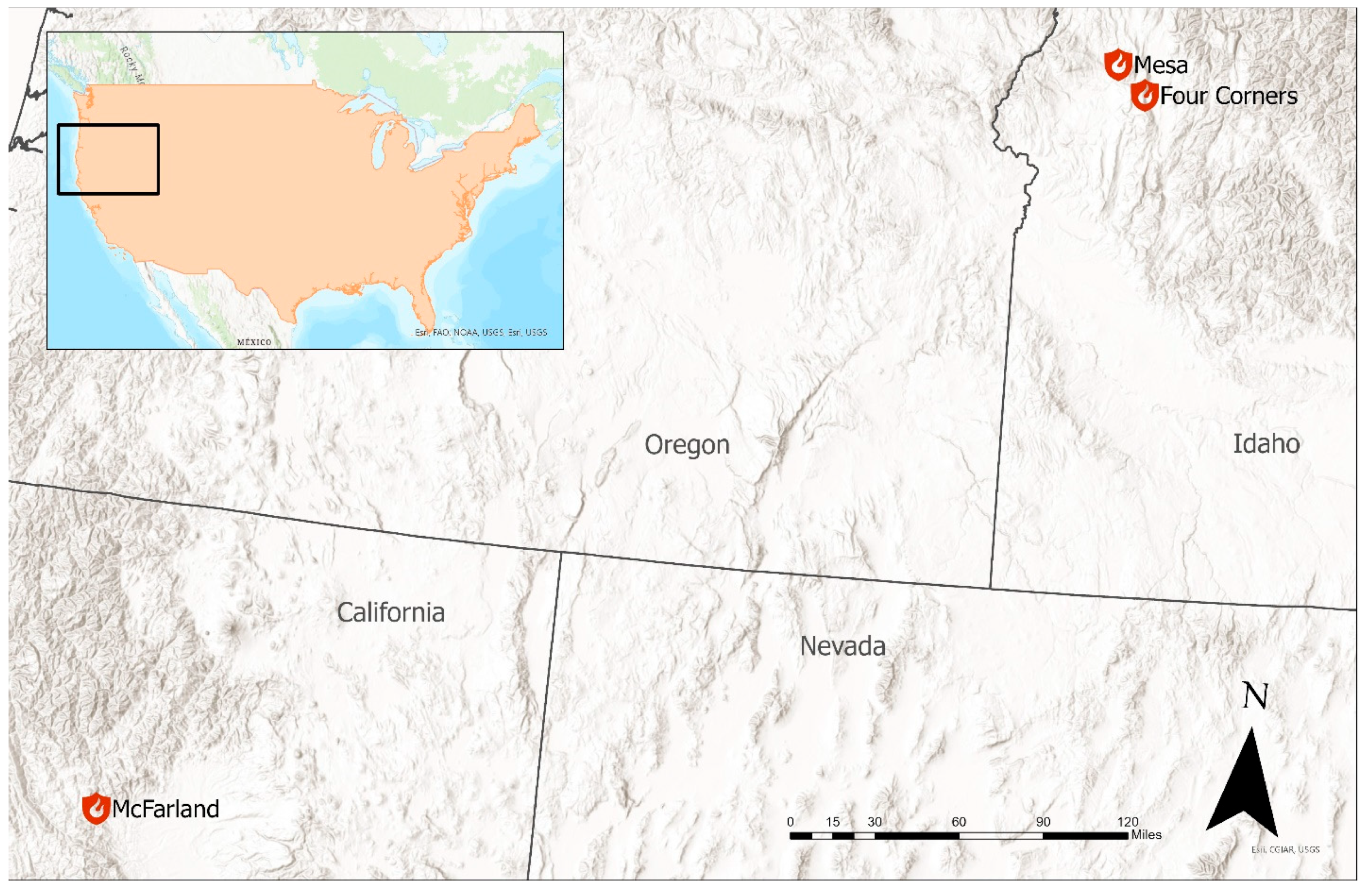
This experiment focused on three study areas, each targeted spatially and temporally on a wildland fire. The first was the Four Corners fire near Cascade, Idaho (at 44.537, −116.169) which started on 13 August 2022, was contained on 24 September 2022, and burned 5556 hectares [35]. The second was the McFarland Fire near Platina, California (at 40.350, −123.034) which started on 30 July 2021, was contained on 16 September 2021, and burned 49,636 hectares [36]. The last was the Mesa Fire near Council, Idaho (at 44.709, −116.348) which started on 26 July 2018, was contained on 25 August 2018, and burned 14,051 hectares [37]. Figure 1 shows the locations of the three study areas relative to each other.
2.2. Imagery
Planet Labs Inc., San Francisco, CA, USA, has launched a constellation consisting of over 200 Dove satellites with the ability to generate up to 200 million square kilometers of PlanetScope imagery a day with the possibility of daily revisits for any particular spot. The original Dove satellites with the PS2.SD sensor captured four bands, while the more recent Super Dove satellites with the PSB.SD sensor capture eight bands, with both satellites ranging from 430 to 890 nm [38]. Even from an altitude of 475 km, PlanetScope spatial resolution manages to achieve three meters with a revisit time of one day [39]. All these characteristics of the Super Dove constellation give it the flexibility to aid researchers in mapping burn extent within the previously referenced fourteen-day window mandated for the completion of burn recovery plans, and it is also able to acquire post-fire imagery before meteorologic conditions such as wind and rain can degrade white ash within the burned area, making it harder to detect areas with higher biomass consumption from the imagery.
PlanetScope imagery was acquired for each of the fires through Planet Lab’s Education and Research Program. For the two more recent fires (McFarland and Four Corners), eight-band imagery was collected with PlanetScope’s PSB.SD sensors. The Mesa Fire burned before the SuperDoves with the PSB.SD sensors were deployed, so four-band imagery from the older Doves with the PS2.SD sensors was used instead. Table 1 contains the image acquisition dates for each of the fires.
The latest PlanetScope sensor deployed on Planet Lab’s Super Dove constellation is the PSB.SD sensor. This sensor uses a butcher block filter, which breaks the frame captured by the satellite’s 47-megapixel sensor into 8 distinct “stripes”, one for each of the eight bands. This frame’s stripes are then combined with adjacent frames to create the final eight-band imagery. Table 2 shows the band names, wavelength, and bandwidth as defined by the full width at half maximum (FWHM) and their interoperability with Sentinel-2 imagery [38].
Prior to the launch of the Dove-R constellation in 2019, Planet Labs deployed the Dove constellation with PS2 sensors in July 2014. The last Dove satellites were decommissioned in April 2022. The PS2 sensor consists of a Bayer pattern filter that separates the wavelengths of light into blue, green, and red channels with a two-stripe filter placed on top. The top stripe of this second filter blocks out near-infrared (NIR) wavelengths, allowing only blue, green, and red light to pass through. The bottom stripe of this second filter allows only the NIR wavelengths to pass through. Similar to the PSB.SD sensors, this creates a striped effect, where the top half of each frame is red, green, and blue (RGB), and the bottom half is NIR. Adjacent frames are combined to produce the final four-band image with RGB and NIR bands (RGB–NIR) [38].
Unmanned aerial system (UAS) imagery was captured over a study area within the Mesa fire while the team was assisting post-fire management efforts by the US Forest Service Rocky Mountain Research Station. While the PlanetScope data has a three meter spatial resolution [40], the UAS is capable of a hyperspatial resolution of just five centimeters (5 cm) [41]. Hyperspatial imagery over the Mesa Fire was only acquired for a 350 hectare area of interest within the fire perimeter. This area of interest corresponded to post-fire fieldwork this team assisted with in the fall of 2018 [13]. Post-fire drone imagery of the Four Corners fire was also acquired as part of this research effort.
This hyperspatial data was captured using a DJI Phantom 4, which carries a three-band color camera, capturing the visible spectra in red, green, and blue bands. Its bands have a mildly different spectral response than red, green, and blue bands found in a typical color camera [42], but is still close enough to be used to capture three-band color images for mapping burn severity [17]. Table 3 shows the comparison of band frequencies between the sensors on the DJI Phantom 4, the Planet Labs Doves, and PlanetLabs Super Doves.
2.3. Feature Engineering
PlanetScope imagery for each of the study areas typically consisted of multiple tiles, which were merged into a single image for an entire burn area for each fire. The tiles were combined using ArcGIS Pro’s Mosaic to the New Raster tool [43]. Each image was input, entering the number of bands (eight for the McFarland and Four Corners Fires, four for the Mesa Fire) and the color type (16-bit unsigned). Once this was done, the data was ready for analysis.
2.3.1. Band Extraction
To assess the utility of each band as an input for classification, the Extract Bands tool within ArcGIS Pro, found under Raster Functions, was used. The Mesa Fire was in 2018, which predates Planet Lab’s deployment of the Super Dove constellation. As a result, imagery with only the red, green, blue, and NIR (RGB–NIR) bands from the PS2 sensors on the Dove Constellation was available for the Mesa Fire. To enable consistency with the Mesa Fire, the RGB–NIR bands for the Four Corners and Mesa Fires were extracted with the ArcGIS Pro Extract Band [44] tool from the eight-band imagery taken by the PSB.SD sensor for both fires.
Three-band imagery with red, green, and blue (RGB) bands was then extracted from the respective four-band RGB–NIR imagery so the experiment could be run with a traditional three-band RGB image, as would be captured with a typical RGB sensor such as that found on the DJI Phantom 4.
2.3.2. Dimensionality Reduction
This study enabled the investigation of which of the PlanetScope bands were most useful to map burn severity. There are a number of metrics, such as normalized burn ratio (NBR) and normalized difference vegetation index (NDVI), which have successfully been used to map burn severity, but each of these relies on a subset of the available bands, making assumptions about which bands are useful. NBR only considers NIR and SWIR while NDVI only utilizes the red and NIR bands. This effort did not make any such assumptions, instead considering all the available bands and leveraging the bands which were found to be most useful for mapping burn severity.
Dimensionality reduction analysis is a method of taking a multidimensional (or multi-feature) dataset and lowering the number of dimensions while retaining as many of the meaningful properties contained in the original data as possible. During training, SVM decision spaces are determined by the input imagery’s band count. For example, eight-band imagery corresponds to an eight-dimensional decision space, while three-band RGB imagery needs a decision space of only three dimensions. However, not all bands are equally helpful in classification. Hamilton [33] showed that in burn extent and severity classification using RGB drone imagery, the blue band yields less information gain than the green and red bands (0.64 vs. 0.79, respectively). This result implies that the bands in Planet Scope imagery may not all provide the same level of information for assisting with the classification of burn extent and burn severity. Two different techniques were used by this study to investigate whether most of the helpful information for classification could be represented in three dimensions or bands.
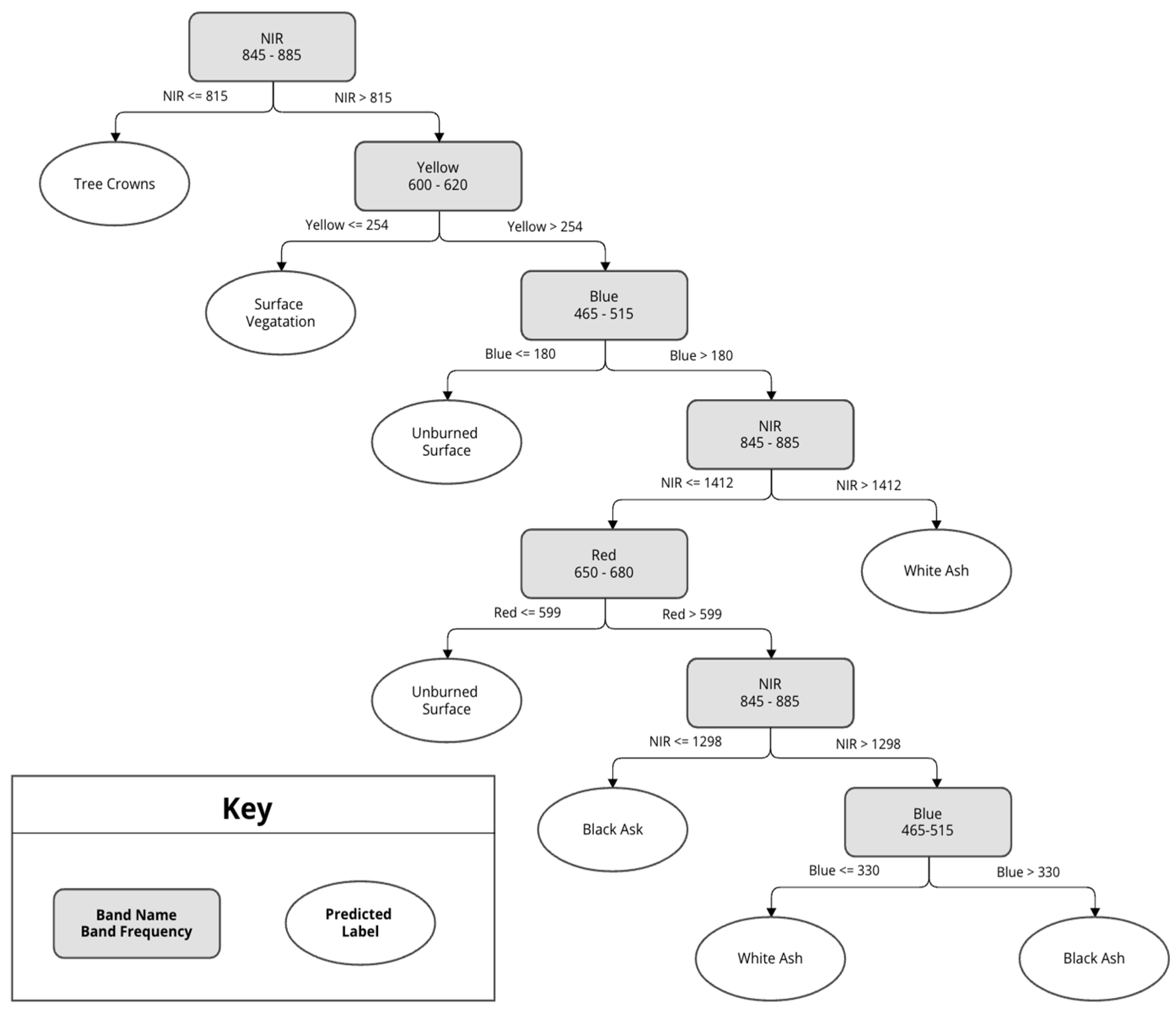
The Iterative Dichotomizer 3 (ID3) is an algorithm that builds a decision tree and splits nodes of the tree based on information gain; that information gain can be used to determine the importance of features during classification. This algorithm was implemented using Sci-kit Learn’s decision tree classifier which implements Gini impurity as the evaluation criterion by default [45]. However, the criterion hyperparameter was set to entropy on the decision tree classifier to evaluate feature importance based on information gain rather than minimization of Gini impurity. Using the ArcGIS Sample tool, the team exported samples containing each of the polygons from the validation dataset, including the band values for the pixels and the class label [46]. The exported samples were fed through the Sci-kit Learn model to build a decision tree and output the usefulness of each band based on its information gain (entropy reduction) while building the tree. The bands resulting in the best information gain were then extracted using the methods in Section 2.3.1. to create a raster with the highest density bands.
For the Mesa fire, the most important band found was red, at 43%; followed by NIR, at 35%; blue, at 13%; and green, at 9%. Therefore, the red, NIR, and blue bands were extracted using the methods in Section 2.3.1. Figure 2 shows a breakdown of the decision tree created by Sci-kit Learn for the Mesa fire’s training samples.
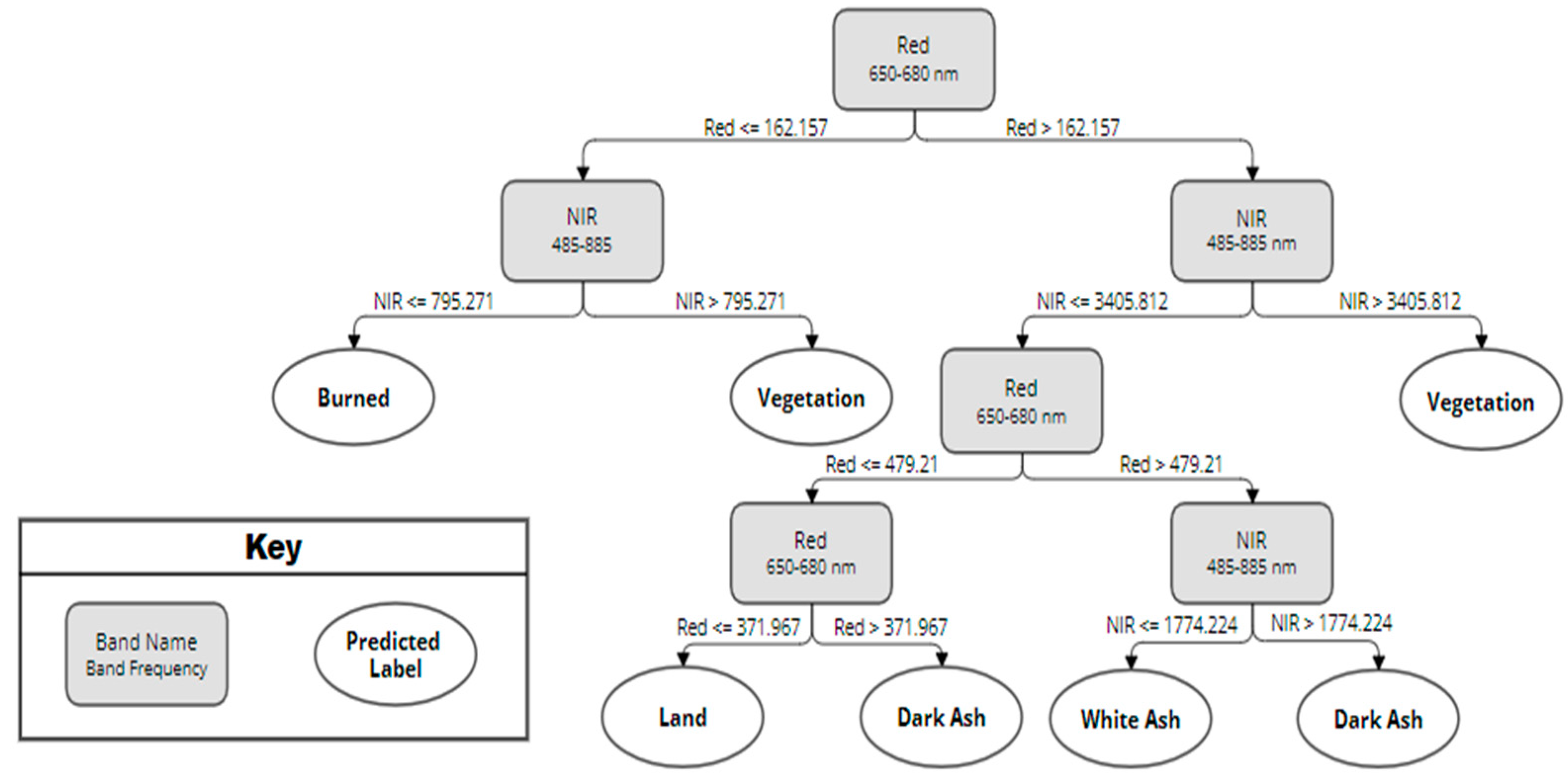
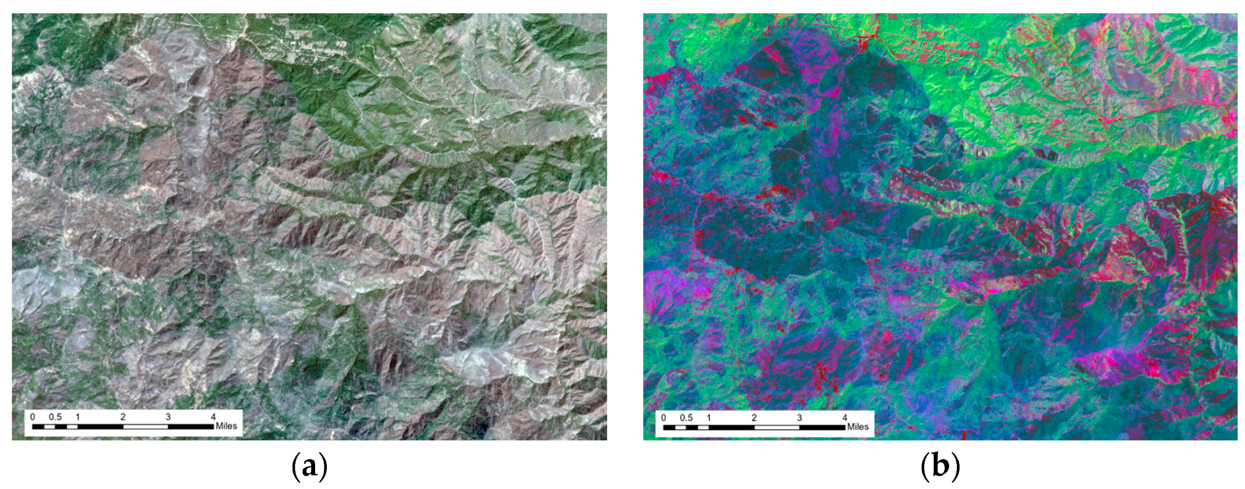
After running the Four Corners eight-band input raster through the ID3 model, two bands, NIR and red, provided roughly 98% of the information gain, while the blue band was the third most helpful, making up the final 2% of information gain. Thus, the remaining coastal blue, green, green 1, yellow, and red-edge bands provided no helpful information in classifying Four Corners according to this classification by the ID3. The decision tree outlining the decision paths leading to label classifications can be seen in Figure 3. The tree has been simplified to display the main paths and decision splits, so only the NIR and red bands are present since they provide 98% of the advantage in classification. A visual depiction of the extracted ID3 bands compared to the RGB bands appears in Figure 4.
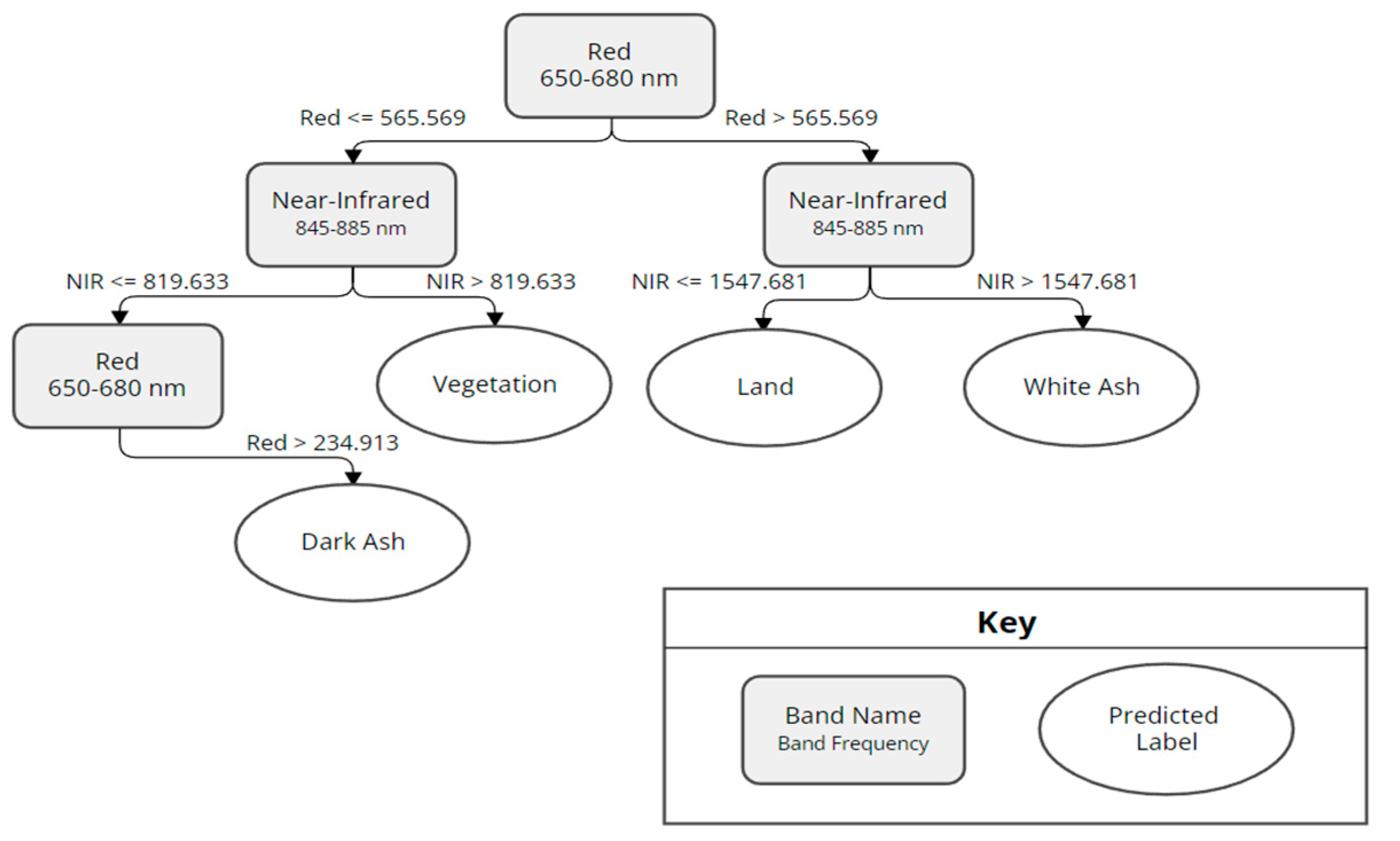
The ID3 results for McFarland look similar to the other study areas, with the NIR band being more useful than any other band. The outputs from this ID3 showed the normalized entropy reduction in the NIR band to be almost 50% alone, with the top three bands of NIR, yellow, and blue holding 98% of the information (yellow at 31% and blue at 17%). Figure 5 shows the decision tree created for the McFarland fire.
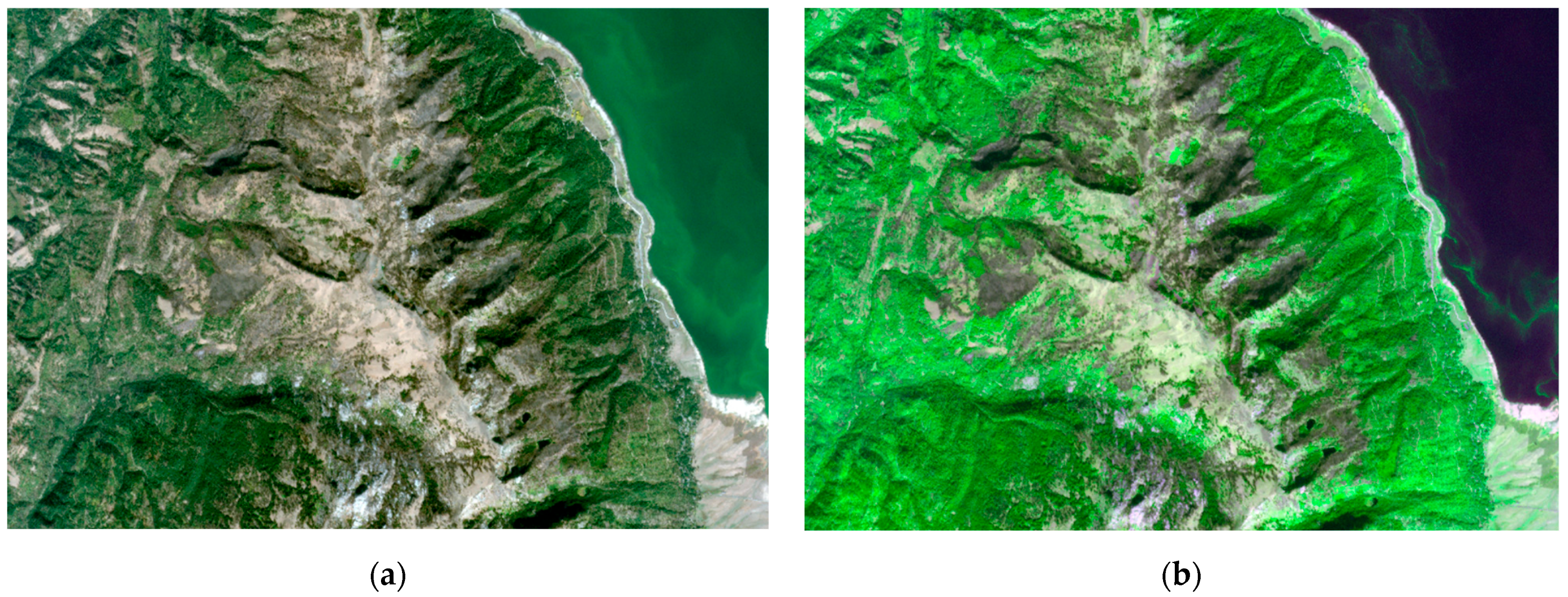
Principal component analysis (PCA) enabled tests of the amount of information that could be retained by taking into account all of the hyperspectral bands and reducing that dimensionality down to three principle components. PCA accomplishes dimensionality reduction by linearly transforming data into a coordinate system in which most variation can be described using only a few initial dimensions. The raster was transformed into three bands using the Principal Components tool in ArcGIS Pro [47]. The Principal Components tool allows a user to input a raster, specify the number of principal components, and then transform the input bands to a new attribute space where the axes are rotated with respect to the original space [31]. Figure 6 shows a comparison between the PCA-transformed bands and the RGB bands of the McFarland Fire.
2.4. Creating Training Data
Once the imagery was acquired and mosaicked into a raster and dimensionality reduction was applied, unique sets of training data were created for each of the Mesa, McFarland, and Four Corners fires to map the burn extent and burn severity. This process was performed in ArcGIS Pro using the Training Samples Manager, which facilitates the digitization of polygons around regions in the image that are denoted as homogeneously containing one of the classes which will be used to train the support vector machine (SVM) [48]. These training polygons were then saved as file geodatabase feature classes in ArcGIS Pro. The training data used to map the burn extent contained burned and unburned classes. The biomass consumption training dataset contained polygons denoting high biomass consumption, as evidenced by white ash, and low biomass consumption, which is noted by the presence of black ash polygons in the black ash class that indicate burned areas that experienced low burn severity. Polygons in the white ash category contained burned areas that experienced high burn severity. These classes separately were used to map burn severity and were combined into a singular “burned” class for mapping burn extent.
Within the unburned class, each fire had unburned vegetation and unburned surface classes. The vegetation class included canopy and surface vegetation, while the surface class contained regions of the image that contained bare dirt (dirt, sand, rocks, and roads, etc.). The rest of the unburned class was partitioned uniquely for each fire. In addition, Four Corners was classified for water since Lake Cascade and the Payette River take up a significant map area, and the Mesa fire had a noise class to deal with errant raster pixels on the edge of the image. Table 4 shows the unburned class partitioning for each of the fires.
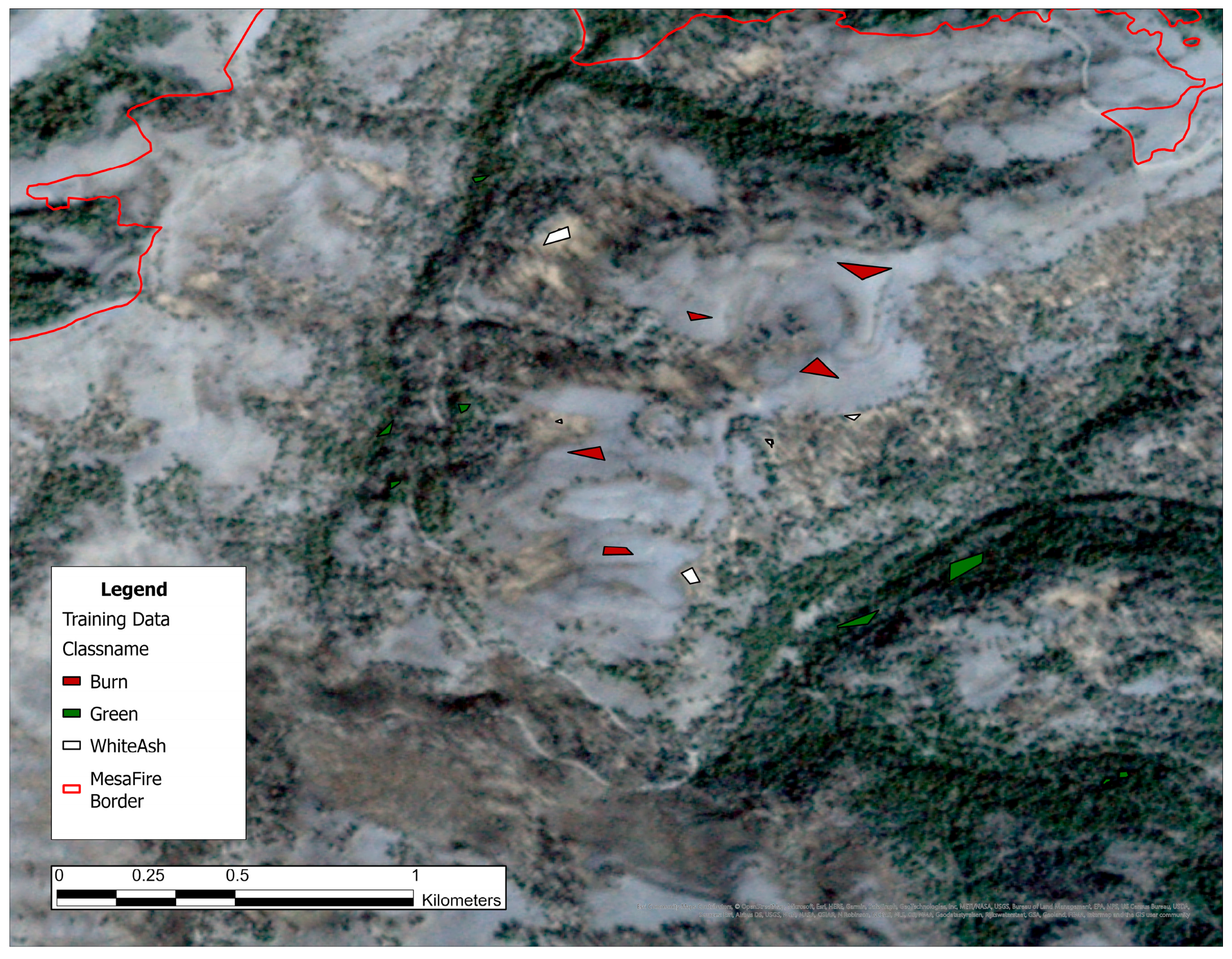
Partitioning the classes beyond burned and unburned was necessary to obtain accurate results from the SVM. SVMs in their simplest form perform binary classification by calculating a hyperplane separating pixels into two classes. It would be difficult for an SVM to identify the hyperplane separating burned and unburned classes due to a wide range of pixel values. For example, the burned class contains low RGB pixel-valued black ash and high RGB pixel-valued white ash. Furthermore, the unburned class is composed of several green, brown, and blue colors whose values vary widely on the RGB scale, but lie between black ash and white ash in the RGB space [17]. To increase spectral difference between classes, the burned and unburned classifications were partitioned into two burned and three or four unburned classes in order to make the individual classes more linearly separable, allowing the SVM to perform multiclass classification. The SVM was able to perform multiclass classification using several hyperplanes with increased accuracy due to the linear separability of the pixel values. After classification, classes were re-generalized back to burned vs. unburned for burn extent and white vs. black ash for burn severity. An example of some training polygons is shown in Figure 7.
2.5. Classification
The support vector machine (SVM) within ArcGIS Pro, found under the Classify tool within the Image Classification toolset [49] was used to map burn extent and severity classifications. The SVM can handle any number of bands as inputs, meaning that we can classify imagery with all available bands, either eight or four, in addition to bands extracted based on decision tree results or engineered with principal component analysis [50]. The following band combinations were used as input when training the SVM:
- Eight-band PlanetScope images (McFarland and Four Corners only)
- Four-band RGB–NIR PlanetScope images
- Three-band-extracted RGB images
- Three-band images transformed by PCA
- Three-band-extracted images based on decision tree band entropy
Table 5 shows the source for each of the sets of classification input rasters.
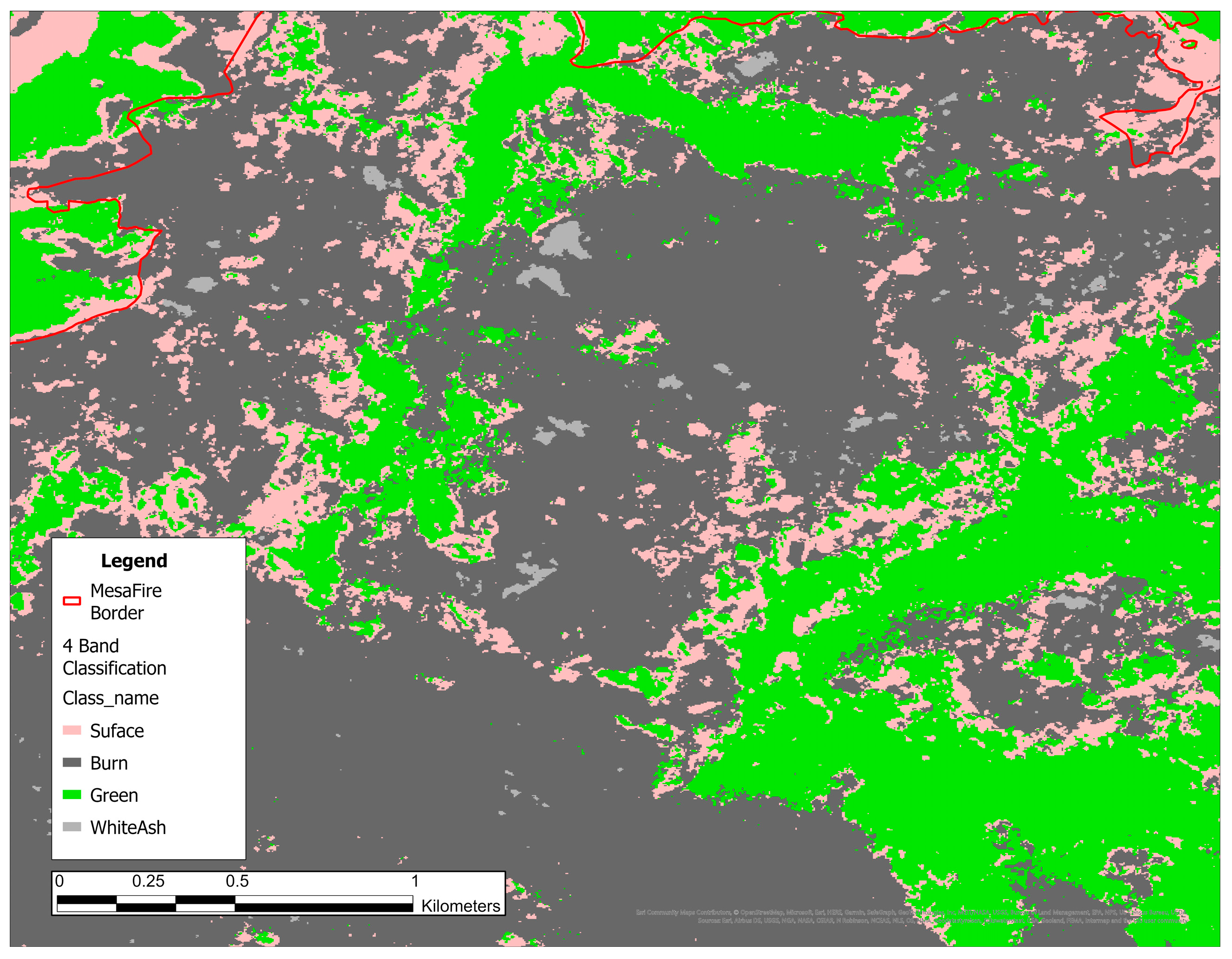
The SVM was trained on images with the previously mentioned set of bands for each of the fires using the training polygons for that specific fire. Once trained on an image, the SVM classified the image, creating the previously mentioned burned (black and white ash) and unburned (vegetation and bare dirt along with water for the Four Corners Fire) layers. To create the burn extent layer for the McFarland and Mesa fires, all burned (white ash and black ash) and unburned (vegetation, land, noise for Mesa) areas were classified and left in their separate classes for validation. Once the images were classified, the ArcGIS Pro Reclassify tool [51] could be used to combine the black and white ash classes into a burned class and the vegetation and bare earth classes back into an unburned class. Figure 8 shows an example of a classification produced by the SVM.
2.6. Validation Data
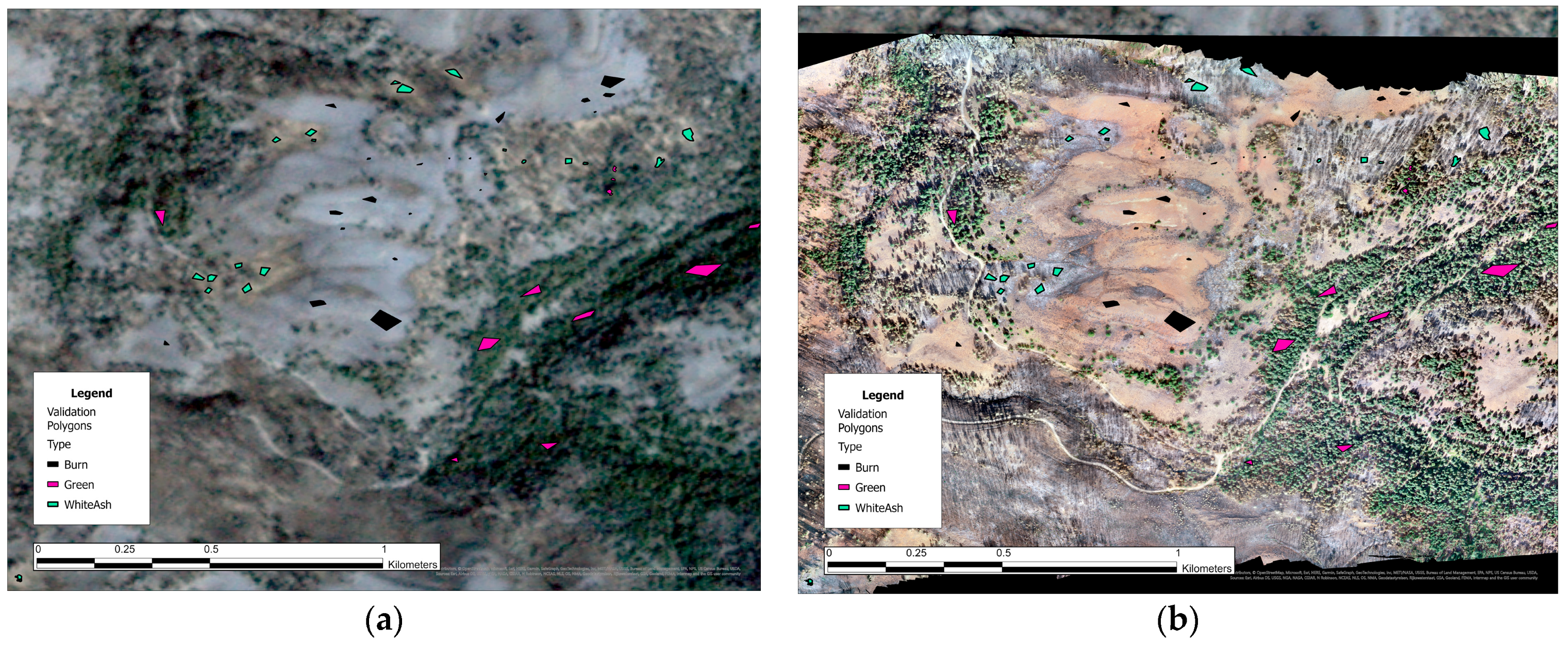
Validation data was drawn to assess the accuracy of the SVM. Using the Create Feature tool in ArcGIS Pro, we created a new raster layer that was made up of several polygons. Each polygon was digitized with 100% certainty of which class it fell under and was labeled with that class. Figure 9 shows a few different validation polygons and their associated classes. Drone imagery for the Mesa Fire was acquired during a previous collaborative effort with the US Forest Service. This hyperspatial drone imagery was used to acquire more precise validation data, which was especially useful when identifying areas of white ash [13], allowing the validation of the Mesa Fire to conform to the International Global Burned Area Satellite Product Validation Protocol [52]. The drone imagery was coregistered with the PlanetScope satellite imagery, which made drawing validation polygons easier, as there was no conversion needed.
2.7. Analysis
Once the team had drawn validation polygons, the appropriate set of validation polygons was fed into the Tabulate Area tool in ArcGIS Pro [53], along with the classified layer of the corresponding imagery. This tool cross-tabulates areas between two datasets and creates a table containing numbers indicating where the datasets overlap. An nxn table was produced, where n represents the number of partitioned classes for the given fire, all representing burned or unburned base classes. This table represents the classification of each pixel using the validation shapefiles and classifier predictions, allowing us to identify where the validation data and predicted data correspond and differ. These were combined into “burned,” which combined black and white ash, and “unburned,” which combined unburned vegetation, unburned surface, and noise. This simplification gave a standard binary 2 × 2 confusion matrix.
Using the confusion matrices, which contain the number of true positives (burned that got classified as burned), false positives (unburned that got classified as burned), true negatives (unburned that got classified as unburned), and false negatives (burned that got classified as unburned), we can calculate accuracy, specificity, and sensitivity based on Equations (1)–(3).
The burn severity classification was evaluated by considering the portion of the confusion matrix dealing with burn pixels, then evaluating these metrics comparing the high biomass (white ash) versus low biomass (black ash) classes.
3. Results
3.1. Burn Extent
For the burn extent, the overall accuracy, sensitivity, and specificity take burned area as the positive class and the unburned area as the negative class. In this case, sensitivity represents the SVM’s ability to identify all the pixels labeled burned by the validation data. Similarly, specificity measures the SVM’s ability to identify areas labeled as unburned by validation data. Accuracy measures the percentage of correct classifications over all pixels, burned or unburned.
3.1.1. Mesa
As Table 6 demonstrates, overall, the SVM was fairly accurate at finding burned area, as demonstrated by the high sensitivity percentage. However, it would often overestimate and over-label what was burned. This high sensitivity to burned areas leads to unburned land being labeled as burned, giving a lower specificity percentage. Overall, the RGB–NIR four-band image, PCA-transformed bands image, and the ID3-informed bands image created good results when they were run through the SVM. However, when the RGB band image was run through the SVM, it over-classified the burned area, which led to very high sensitivity but terrible specificity and an overall fairly low accuracy.
3.1.2. Four Corners
The SVM classifier resulted in an average accuracy of 92.27% across all five of the input layers, as can be seen in Table 7. The lowest accuracy was the RGB layer at 68.05%, which is reasonable, as it had the least information, such as the number of bands, and was not the result of any band utility analysis. With the extra near-infrared (NIR) band, the four-band RGB–NIR layer achieved the third highest accuracy of the Four Corners layers, at 93.46%. One might expect the eight-band layer, adding yellow, coastal blue, red-edge, and green 1, to improve this accuracy. However, the accuracy dropped to 92.66%. As seen in the ID3 results, the NIR, red, and blue bands contributed most of the information in determining appropriate labels. Adding bands such as coastal blue, green 1, red-edge, and yellow did not provide enough information gain in classification and likely confused the SVM, as the eight-band layer wasn’t as accurate as the RGB–NIR layer. Additionally, the two highest accuracy layers are the ID3-informed (NIR, red, and blue) layer, coming in at 94.27%, and the PCA-transformed layer, with an accuracy of 94.93%.
The relative ranking of sensitivity scores across layers is the same as the accuracy results. The RGB layer sits at around 80% sensitivity while the other layers all are close to 98% or above. This indicates that the NIR band improves the classification of burned area by around 18%, while utilizing all bands in eight-band imagery is slightly less useful. Analyzing band information gain with the ID3 algorithm and using the top three bands as well as performing dimensionality reduction with PCA on all eight-bands is shown to be the most effective at classifying burned area.
The RGB layer’s specificity is 88.50%, and the remaining layers are only 2–4% greater. Based on both the 7.5% increase from sensitivity to specificity for RGB and the roughly 6–7% decrease in all other layers, the team hypothesizes that the multispectral coastal blue, green 1, yellow, and NIR bands identify burned area almost too frequently while RGB bands alone can fail to identify certain burned pixels. Unlike sensitivity, specificity measures false positives. The SVM classified several land pixels as burned area likely due to the spectral similarity of some light dirt and white ash, which is included in the burned class.
3.1.3. McFarland
Table 8 shows each input raster’s accuracy, sensitivity, and specificity. All of the inputs yielded results with an accuracy of over 80%. However, only the four-band RGB–NIR input crossed the threshold of 95%. In addition, RGB–NIR four-band imagery had a much higher sensitivity than any other inputs, though the specificity dropped.
Four-band imagery produced excellent SVM classification results. This may be because the NIR band was the most information-dense. The other, less information-dense bands, such as coastal blue and green edge, are more of a distraction, reducing the effect that the NIR band has on determining burned areas. The specificity of the four-band imagery dropped because it was over-classifying white ash specifically. The SVM classified white ash in most of the other inputs as surface, but the four-band imagery did the opposite, classifying surface (white rocks specifically) as white ash.
3.2. Burn Severity
3.2.1. Mesa
Overall, the SVM classified the Mesa fire well. All four images run through the SVM had about the same results. It performed relatively well when finding areas of white ash and would rarely label something as white ash that was not, achieving an average specificity score of 98.89%. However, much like when finding burn extent, it was often biased when labeling black ash and labeled more pixels as black ash than were actually black ash. This aggressiveness leads to a low sensitivity score of 74.15% on average. The overall accuracy averaged out to approximately 85.88%. As Table 9 demonstrates, there was very little variance in accuracy between the different images when classified.
3.2.2. Four Corners
Overall, the SVM was able to classify light versus dark ash with an average accuracy across layers of 96.45%, as shown in Table 10. This should be expected, given the large spectral differences between white and black ash, as noted by Hamilton [17]. It may be surprising as well to see that the RGB layer had the highest accuracy, but this is intuitive, as RGB represents human visibility and humans can easily detect differences between white and black color. Further, it seems adding bands does not improve this obvious spectral separability but rather hinders it, as observed in the lower accuracies of the remaining four layers. Additionally, black ash pixels were identified correctly as black ash 100% of the time across all layers, but white ash pixels were sometimes missed. Sensitivities in the RGB and RGB–NIR layers were the highest, meaning they identified white ash correctly more often than the other three layers. The overall sensitivity is 91.61% compared to the 100% average specificity, showing that across all layers, the SVM occasionally misidentified white ash as black ash, but never misidentified black ash as white ash.
3.2.3. McFarland
When observing the accuracy, specificity, and sensitivity of burn severity (black ash vs. white ash) assessment of the McFarland fire, these metrics were all at or around 100%. Based on this, the team determined that, at least for the McFarland fire, the classifier was nearly perfect for distinguishing black ash from white ash. This was not surprising, given the massive spectral differences between black ash and white ash, as observed by Hamilton [17] and the obvious difference between white and black ash. The imagery of the McFarland fire contains a lot of white rock, which makes classifying white rock (unburned surface) vs. white ash (high biomass consumption) incredibly difficult. More than 50% of the white ash validation polygons were classified as surface, though surprisingly, next to none of the surface was classified as white ash. The differences between white ash and black ash are distinct enough that they were not confused, because almost everything that is too light to be black ash was often classified as surface.
In Table 11, the true positive was white ash which was correctly classified as white ash and the true negative was everything else which was correctly classified as anything except white ash. The false positive was any other class that got incorrectly classified as white ash and the false negative was the white ash that got incorrectly classified as anything else. This change led to much more comparable results to other fires. It also accounts for the white ash being classified as surface.
The sensitivity values show how much white ash was correctly classified as white ash, with most of them below 50% accuracy. The only image that really stands out from the group is the four-band RGB–NIR image. This table has the opposite problem, as it doesn’t show white ash as well, although Table 12 shows the issue slightly better.
The middle column of Table 12 is the same as the sensitivity in Table 11, but the new column on the right shows how many pixels are incorrectly attributed as white ash. In all of these scenarios, the only parts being incorrectly classified are white ash as surface (first column) or surface as white ash (second column). As seen before, the four-band RGB + NIR imagery was the best at correctly identifying white ash, though it was an overly biased classification, classifying a fairly large amount of unburned surface as white ash. It classified more than any other class. Even with this misclassification of white soil as white ash, the metrics were not adversely affected due to how much of the white ash was correctly classified.
The ID3-informed bands still had a number of issues. They were the only input that misclassified white ash in both directions. Not only did it classify most of the white ash as surface, but it also classified a fairly large portion of the surface (roughly 20%) as white ash. Put together, these issues compounded to create the lowest accuracy, sensitivity, and specificity of any input.
4. Discussion
4.1. Results Analysis
4.1.1. Burn Extent
Across the Mesa, McFarland, and Four Corners fires, excellent average accuracies were obtained using various input layers, as shown in Table 13. An average accuracy of 89.50% was obtained across the three fires and five layers, with RGB–NIR being accurate at an average of 92.06% across the three fires. These averages show a significant increase from the 84.90% average accuracy for the RGB results, which follows the theory that more spectral bands lead to higher accuracy in SVM predictions. The eight-band imagery yielded a classification accuracy of 90.87% for the two fires (McFarland and Four Corners) for which eight-band imagery was available. While incredibly close to the RGB–NIR imagery’s precision, the eight-band imagery is slightly less accurate. Further, the PCA-transformed and ID3-informed imagery yielded even lower accuracies than the RGB–NIR by a larger margin, at 90.63% and 89.04%, respectively. However, this is not out of the ordinary, as both PCA and the ID3 are forms of dimensionality reduction, which inherently leads to some information loss.
The average sensitivity for all sets of input bands between the fires averaged 88.81%. RGB–NIR was the highest by far, at 96.85%. This shows that the SVM used the NIR band the most to identify the burned areas in the experiment accurately. Given that RGB imagery and imagery with or informed by higher bands performed at around 85–87% sensitivity, the extra coastal blue, green 1, yellow, or red-edge bands likely caused the SVM to misidentify some burned areas as unburned. The RGB layer demonstrates that without the NIR band the classification of burned area is no better than when it is confused by extra bands, so the optimal layer for identifying burned area is RGB–NIR.
The specificity results are opposite to the sensitivity results. The top layer is the eight-band followed by PCA-transformed and ID3-informed bands. A combination of RGB and NIR bands is not enough to identify unburned areas in contrast to burned.
Table 14 contains the breakdown of each fire’s accuracy, sensitivity, and specificity assessments across all input layers relevant to the respective fire. McFarland and Four Corners had the highest overall accuracies at 89.81% and 92.27%, respectively. Additionally, McFarland had a specificity higher than its accuracy and lower sensitivity, while Mesa exhibited the opposite trend with a higher sensitivity and lower specificity with a margin of about +/− 8% compared to the accuracy. Across all spectral resolutions, the SVM often misclassified unburned areas as burned because of shadows, leading to low specificity. McFarland’s low sensitivity can be explained by its misclassification of white ash as unburned surface. These issues are covered in Section 4.4.
4.1.2. Burn Severity
The burn severity experiment results are comparable to that of the burn extent experiment, albeit with more variance. The overall accuracy across all input layers and all three fires is nearly 91.2%, with sensitivity down to 74.52% and specificity at an extremely high 98.74%, as shown in Table 15. Eight-band imagery, only for McFarland and Four Corners, classified white ash with a sensitivity of 66.28% but yielded an essentially perfect 99.96% specificity. This is similar to the burn extent results where the eight-band imagery scored lowest in sensitivity but highest in specificity.
In comparing the average results from the three fires, as shown in Table 16, the team noticed that McFarland’s average accuracy is slightly higher than Mesa’s, with Four Corners yielding the highest results in any metric. As discussed in Section 3.2.3, the sensitivity of McFarland’s burn severity results is much worse than any other fire, most likely due to the prevalence of white rocks across the imagery. Specificity scores are incredibly high for all three fires, indicating that black ash was easier for the SVM to accurately identify than white ash.
Mesa’s lower accuracy appears to be because a large portion of the validation data for burn severity was acquired using the 1000 acres of 5 cm resolution drone imagery. As discussed later in the discussion section, this makes it easy to draw validation data over areas that the 3 m pixels could not pick up. While this does lead to a lower accuracy on paper, this may be a good thing for the experiment. This result confirms the value of having higher resolution imagery available for validation of burn products [52]. A future effort could prove that having a higher resolution image for classification may lead to much higher accuracy, even when compared to validation data drawn on hyperspatial imagery.
4.2. Problems with Shadows
Shadows proved to be a limiting factor when the SVM classified burned areas. Pixel RGB values of shadows and dark burned ash are similar, causing the SVM to classify shadows as unburned. Humans can identify that the area classified as burned outside of the fire boundary is a shadow, often of mountain ridges. In imagery taken early in the morning, the sun was lower in the sky, casting shadows throughout the image. The SVM cannot distinguish between this the same way humans can, so several false positives were created during classification and hurt specificity [54]. RGB exhibits this specificity decline due to false positive shadows. However, the addition of multispectral bands such as near-infrared, coastal blue, green 1, and red-edge increased specificity. This increase indicates that the additional bands may contain information distinguishing shadow from burn that is not observable with RGB bands.
Within the burned boundary of Four Corners, many extremely dark sections were unable to be conclusively identified as vegetation or dark ash. By observing the topographical map, these regions were identified as north-facing slopes, increasing the likelihood that they were shadows. Additionally, observing pre-fire imagery showed that these regions were darker than their surroundings before the burn had begun, strongly indicating that the dark hue was due to shadow. Because of this complication, these regions needed to be omitted from training and validation data, as they could not be confirmed as vegetation or dark ash.
4.3. Using Drone Imagery
Most of the validation data for the Mesa Fire, especially for white ash, came from the drone imagery that was taken over a small portion of the fire. While drone imagery made the validation area significantly easier, it also created some issues and made the accuracy of the classified data over the Mesa fire seem lower than it should be. The first issue was the spatial resolution of drone imagery compared to the satellite imagery the SVM is run on. The drone imagery has a spatial resolution of five centimeters per pixel, which is about 60 times better than the PlanetScope imagery from Planet Lab’s Dove and Super Dove satellites, which have a spatial resolution of around 3 m. While the 3 m satellite imagery is fairly good for identifying burned and unburned areas, it cannot compete when comparing and validating it with drone imagery. This leads to the accuracy being comparatively low compared to the Four Corners and McFarland fires, especially when looking at burn severity and white vs. black ash.
Drone imagery was also used to confirm the presence of white ash and burned area for the Four Corners fire. The team was not able to gain access to the site until the following summer; consequently, the team found ground truth observations to be more useful than drone imagery, especially for detection of what white ash was still present at that time. Looking at Planet Scope’s three-meter imagery, many areas appear to be a certain class, whether that be white ash or black ash, but it is hard to be conclusive, as the three-square-meter spaces were very heterogenous. Getting a closer visual using the same drone imagery as well as ground truth observations allowed the team to confirm the conclusions that were drawn from the satellite imagery.
4.4. Issues with White Ash in the McFarland Fire
The team determined that white ash was the main reason behind the decreased accuracy and sensitivity of assessments of the McFarland fire. For most of the inputs, white ash was classified as bare earth due to the abundance of white rocks in the McFarland fire imagery. However, four-band imagery accurately classified almost all the white ash, although it incorrectly classified some surface as white ash.
4.4.1. Spatial Resolution
The team’s first hypothesis for why this occurred is that the spatial resolution may be too low. As mentioned in the Materials and Methods section, the PlanetScope Super Dove imagery has a spatial resolution of 3 m. As discussed in Section 4.3, the hyperspatial drone imagery was incredibly useful in validating black ash vs. white ash. This was backed up by both the drone imagery used in the Mesa fire and the ground truth observations made in the Four Corners fire. This study hypothesizes that hyperspatial resolution is needed to accurately distinguish white ash from light-colored surfaces. While 3 m satellite data is incredibly useful, it is not quite as useful as a higher resolution image.
4.4.2. Spectroscopy
The second hypothesis posed by the team is that the spectral difference between white ash and the white rocks may have been a cause of this incorrect classification. The imagery provided by the PlanetScope Super Dove satellites ranges from the wavelengths of 431–885 nm. Based on the conclusions of Hamilton [17], the reflectance of white ash is even, at roughly 30–40% across that entire range. The white rock showing up in the images is most likely quartz diorite, as shown by a geological survey of the area [55]. As shown in [56], the reflectance of a diorite substance with trace amounts of quartz is very similar along these same wavelengths, roughly in the 30 percent range. This study supposes that hyperspectral imagery may be beneficial to accurately distinguish between white ash and these light-colored rocks.
4.4.3. Temporal Resolution
The third possibility is that white ash is just too volatile to be picked up, even with PlanetScope’s very impressive temporal resolution. White ash is easily degraded by a number of meteorological factors, including wind and rain. In the McFarland fire specifically, this seems like a rather unlikely explanation, due to the imagery being collected within a week of the fire’s containment, but it is an important note while doing further research or putting these methods into practice.
4.4.4. Concluding Thoughts on McFarland and White Ash
The best hypothesis for why the white ash on McFarland was so hard to acquire accurately is addressed in both the Spatial Resolution (Section 4.4.1) and the Spectroscopy (Section 4.4.2). At 3 m, it is a bit difficult to confidently identify white ash when digitizing validation polygons. The methodology the team resorted to for identifying white ash in the McFarland fire supposed that anything that appeared white within the burned area and showed up as green in the pre-fire imagery should be labeled as white ash. This resulted in the team members who digitized the white ash polygons not being fully confident while drawing training and validation polygons. This, compounded with the fact that both the white stones and white ash appear to have similar metrics of reflectance, is what the team believes led to the rather low results found for McFarland.
4.5. ID3 Issues in McFarland
One thing the team noticed was the fact that, for the McFarland fire specifically, the ID3-informed bands performed quite a bit worse than any other input that was used. While both other fires had their ID3′s return results similar to other inputs (just below 90% for Mesa and roughly 99% for Four Corners), the McFarland fire took a noticeable dip in accuracy. With most of the others being about 90% accurate, disregarding the outlier of the RGB + NIR at 96%, the ID3-informed bands performed at only 84% accuracy. The team is unsure of the reason for the discrepancy. The ID3 decision tree itself returned similar bands to other fires, with NIR being the highest, yellow being the second, and blue being third. Outside of that, the only other band that was used in the tree was the red band, which was fairly low compared to the other three.
Given the nature of NIR making up over 50% of the information gained according to the ID3, the team was fully expecting this set of bands to perform the best overall. In the case of both other fires, the ID3 performed as expected, but for McFarland, the accuracy and especially the specificity were negatively affected when considering the burn extent. Both of these seemed to be related to white ash specifically, and it became obvious when assessing burn severity that the white ash was indeed the issue. For whatever reason, the white ash problem discussed in Section 4.4. was only compounded with the ID3 data. It both over-classified a vast majority of white ash as unburned surface and classified about 20% of the unburned surface as white ash. Put together, the issues compounded to affect both the burn extent and burn severity results.
The team is unsure of what caused these results to occur. Some possibilities include the fact that this is a form of dimensionality reduction, which inherently cuts out some data. Alternatively, three bands may not be enough to include all the data, especially when dealing with such minor differences between white ash and white rocks. According to the findings of Zhou and Wang [56], the only wavelengths with any substantial amount of spectral difference between white ash and quartz diorite exist at the extreme lows near the coastal blue band and extreme highs, which are outside the range of bands available with PlanetScope imagery. It is possible that, in cutting out the coastal blue band, the only band with enough spectral difference to correctly classify white ash against the white rocks may have been lost.
5. Conclusions
The use of satellite imagery from high spatial resolution satellites such as PlanetScope allows for the burn extent and severity to be mapped without the intensive endeavor of capturing drone imagery and creating the mosaics by hand. Using satellite imagery instead of drone imagery is especially important when dealing with large fires such as the fires classified in this research. The three fires that were used in this research are the Mesa Fire, McFarland Fire, and the Four Corners Fire. RGB, RGB–NIR, PCA-transformed and ID3-informed imagery were used for each fire along with eight-band imagery for the McFarland and Four Corners fires due to the fires burning after PlantScope SuperDoves were launched. Feeding these layers through a support vector machine, it was shown that the near-infrared band is the most useful band in both burn extent and burn severity classification. Additional bands from the PlanetScope SuperDove imagery such as coastal blue, green 1, and yellow did not provide much, if any, information gain during classification.
Future Work
While the central goal of this project was to focus on local variables and determine the best factors for each fire on a local level, there has been work on attempting to train a model that can classify fires on a global level. In previous work by Hamilton [54], there was an attempt to classify multiple fires using a single training data set. However, the accuracy took a significant drop in their attempts. Our current research is determining what works best on a local scale and training and classifying one fire at a time before attempting to classify multiple fires at once again. Therefore, future work in this field of research will require taking what was learned in this project and using it to classify multiple fires in one training data set.
Spatial resolution is not the only consideration when identifying burned and unburned land. So far, this project has used drone imagery with extremely high spatial resolution but low spectral resolution and PlanetScope Dove and Super Dove satellites with high spatial resolution and medium spectral resolution. Planet Labs does have other platforms that could help improve spatial resolution. For example, Planet Lab’s new Tanager satellites scheduled to be launched in 2024 allow for high spectral resolution with over 400 different bands at 5 nm spacing [57]. The high spectral resolution could help with addressing problems in the imagery, such as shadows. However, they have incredibly low spatial resolution, with 30 m per pixel. This high spectral resolution could be used in a future project comparing the importance of spectral vs. spatial resolution.
Another option for future work is revisiting higher spatial resolution. One way to do this would be using PlanetLab’s SkySat satellites. These satellites have 50 cm spatial resolution and take sub-daily images [57]. However, these satellites have a fairly low spectral resolution and can only take four-band imagery. Using SkySat in future work could allow for the utilization of very high spatial resolution but low spectral resolution satellite imagery. Another option when going down the path of high spatial resolution is Planet Lab’s Pelican satellites. These satellites are scheduled to be launched in early 2023 and will provide 30 cm imagery with seven bands of spectral resolution [58]. These satellites could add a massive increase in the spatial resolution of satellite imagery while keeping a seven-band spectral resolution. Exploring more options with various spectral and spatial resolutions is a future task in this field that will enable identifying the importance of each type of resolution when mapping wildfires. Conversely, freely available Sentinel-2 imagery with higher spectral resolution and extent could also be evaluated to further assess the impact of the tradeoff between spectral resolution and extent versus spatial resolution, as could the Landsat Next satellite when it is launched in 2030, capturing 26 bands at 10 to 20 m spatial resolution with a revisit time of six days [59].
Author Contributions
Conceptualization, D.H. (Dale Hamilton); methodology, D.H. (Dale Hamilton); software, C.M., D.H. (Daniel Harris) and W.G.; validation, C.M., D.H. (Daniel Harris) and W.G.; formal analysis, C.M., D.H. (Daniel Harris) and W.G.; investigation, D.H. (Dale Hamilton), C.M., D.H. (Daniel Harris) and W.G.; resources, D.H. (Dale Hamilton), C.M., D.H. (Daniel Harris) and W.G.; data curation, C.M., D.H. and W.G.; writing—original draft preparation, D.H. (Dale Hamilton), C.M., D.H. (Daniel Harris) and W.G.; writing—review and editing, D.H. (Daniel Harris), W.G., C.M. and D.H. (Dale Hamilton); visualization, C.M., D.H. (Daniel Harris) and W.G.; supervision, D.H. (Dale Hamilton); project administration, D.H. (Dale Hamilton); funding acquisition, D.H. (Dale Hamilton). All authors have read and agreed to the published version of the manuscript.
Funding
This research was funded by Idaho NASA EPSCoR under award 80NSSC19M0043.
Data Availability Statement
All data and source code from this project is available at https://firemap.nnu.edu/PS_Burn_Severity (accessed on 20 July 2023.)
Acknowledgments
We would like to acknowledge Planet Labs Inc. for making imagery for this effort available through their Education and Research Program. We would like to also acknowledge the students in the Northwest Nazarene University department of Math and Computer Science who have helped with different aspects of this effort, including current and former students Cole McCall, Kedrick Jones, Adrian De Orta, and Elliott Lochard. Additionally, we would like to thank Leslie Hamilton and Catherine Becker for reviewing and editing this manuscript.
Conflicts of Interest
The authors declare no conflict of interest.
References
- Abatzoglou, J.T.; Williams, A.P. Impact of anthropogenic climate change on wildfire across western US forests. Proc. Natl. Acad. Sci. USA 2016, 113, 11770–11775. [Google Scholar] [CrossRef] [PubMed]
- Keeley, J.E.; Syphard, A.D. Twenty-first century California, USA, wildfires: Fuel-dominated vs. wind-dominated fires. Fire Ecol. 2019, 15, 24. [Google Scholar] [CrossRef]
- Wildland Fire Leadership Council. The National Strategy: The Final Phase in the Development of the National Cohesive Wildland Fire Management Strategy. 2014. Available online: https://www.forestsandrangelands.gov/documents/strategy/strategy/CSPhaseIIINationalStrategyApr2014.pdf (accessed on 23 September 2021).
- Hoover, K.; Hanson, L.A. Wildfire Statistics. Congressional Research Service. 2022. Available online: https://crsreports.congress.gov/product/pdf/IF/IF10244 (accessed on 10 February 2023).
- National Interagency Fire Center. Suppression Costs. Available online: https://www.nifc.gov/fire-information/statistics/suppression-costs (accessed on 10 February 2023).
- National Wildfire and Coordinating Group. NWCG Report on Wildland Firefighter Fatalities in the United States: 2007–2016. 2017. Available online: https://www.nwcg.gov/sites/default/files/publications/pms841.pdf (accessed on 10 February 2023).
- Zhou, G.; Li, C.; Cheng, P. Unmanned aerial vehicle (UAV) real-time video registration for forest fire monitoring. In Proceedings of the 2005 IEEE International Geoscience and Remote Sensing Symposium, 2005, IGARSS ’05, Seoul, Republic of Korea, 29 July 2005. [Google Scholar] [CrossRef]
- Insurance Information Institute. Facts + Statistics: Wildfires. Available online: https://www.iii.org/fact-statistic/facts-statistics-wildfires (accessed on 5 September 2023).
- Eidenshink, J.C.; Schwind, B.; Brewer, K.; Zhu, Z.-L.; Quayle, B.; Howard, S.M. A project for monitoring trends in burn severity. Fire Ecol. 2007, 3, 3–21. [Google Scholar] [CrossRef]
- Planet Team. Planet Application Program Interface: In Space for Life on Earth. Planet. Available online: https://api.planet.com (accessed on 9 May 2023).
- Hamilton, D. Improving Mapping Accuracy of Wildland Fire Effects from Hyperspatial Imagery Using Machine Learning; The University of Idaho: Moscow, ID, USA, 2018. [Google Scholar]
- National Aeronautics and Space Administration (NASA). Landsat 9 Instruments. NASA. Available online: http://www.nasa.gov/content/landsat-9-instruments (accessed on 13 February 2023).
- Lewis, S.A.; Robichaud, P.R.; Hudak, A.T.; Strand, E.K.; Eitel, J.U.H.; Brown, R.E. Evaluating the Persistence of Post-Wildfire Ash: A Multi-Platform Spatiotemporal Analysis. Fire 2021, 4, 68. [Google Scholar] [CrossRef]
- Keeley, J.E. Fire intensity, fire severity and burn severity: A brief review and suggested usage. Int. J. Wildland Fire 2009, 18, 116–126. [Google Scholar] [CrossRef]
- Key, C.H.; Benson, N.C. Landscape Assessment (LA) Sampling and Analysis Methods; U.S. Department of Agriculture: Washington, DC, USA, 2006; Volume 164. Available online: https://www.fs.usda.gov/research/treesearch/24066 (accessed on 28 April 2023).
- Hudak, A.T.; Ottmar, R.D.; Vihnanek, R.E.; Brewer, N.W.; Smith, A.M.S.; Morgan, P. The relationship of post-fire white ash cover to surface fuel consumption. Int. J. Wildland Fire 2013, 22, 780–786. [Google Scholar] [CrossRef]
- Hamilton, D.; Bowerman, M.; Colwell, J.; Donahoe, G.; Myers, B. A Spectroscopic Analysis for Mapping Wildland Fire Effects from Remotely Sensed Imagery. J. Unmanned Veh. Syst. 2017, 5, 146–158. [Google Scholar] [CrossRef]
- Lentile, L.B.; Holden, Z.A.; Smith, A.M.; Falkowski, M.J.; Hudak, A.T.; Morgan, P.; Lewis, S.A.; Gessler, P.E.; Benson, N.C. Remote sensing techniques to assess active fire characteristics and post-fire effects. Int. J. Wildland Fire 2006, 15, 319. [Google Scholar] [CrossRef]
- Alcaras, E.; Costantino, D.; Guastaferro, F.; Parente, C.; Pepe, M. Normalized Burn Ratio Plus (NBR+): A New Index for Sentinel-2 Imagery. Remote Sens. 2022, 14, 7. [Google Scholar] [CrossRef]
- Escuin, S.; Navarro, R.; Fernandez, P. Fire severity assessment by using NBR (Normalized Burn Ratio) and NDVI (Normalized Difference Vegetation Index) derived from LANDSAT TM/ETM images. Int. J. Remote Sens. 2008, 29, 1053–1073. [Google Scholar] [CrossRef]
- Chuvieco, E. Fundamentals of Satellite Remote Sensing: An Environmental Approach; CRC Press: Boca Raton, FL, USA, 2016. [Google Scholar]
- Brown, M.E.; Pinzón, J.E.; Didan, K.; Morisette, J.T.; Tucker, C.J. Evaluation of the consistency of long-term NDVI time series derived from AVHRR, SPOT-vegetation, SeaWiFS, MODIS, and Landsat ETM+ sensors. IEEE Trans. Geosci. Remote Sens. 2006, 44, 1787–1793. [Google Scholar] [CrossRef]
- Holden, Z.A.; Morgan, P.; Smith, A.M.; Vierling, L. Beyond Landsat: A comparison of four satellite sensors for detecting burn severity in ponderosa pine forests of the Gila Wilderness, NM, USA. Int. J. Wildland Fire 2010, 19, 449–458. [Google Scholar] [CrossRef]
- Ononye, A.E.; Vodacek, A.; Saber, E. Automated extraction of fire line parameters from multispectral infrared images. Remote Sens. Environ. 2007, 108, 179–188. [Google Scholar] [CrossRef]
- Deering, D.W. Rangeland Reflectance Characteristics Measured by Aircraft and Spacecraft Sensors. Ph.D. Thesis, Texas A&M University, College Station, TX, USA, 1978. [Google Scholar]
- Han, J.; Kamber, M.; Pei, J. Data Mining: Concepts and Techniques, 3rd ed.; Morgan Kaufmann: Amsterdam, The Netherlands, 2012. [Google Scholar]
- Hamilton, D.; Levandovsky, E.; Hamilton, N. Mapping Burn Extent of Large Wildland Fires from Satellite Imagery Using Machine Learning Trained from Localized Hyperspatial Imagery. Remote Sens. 2020, 12, 24. [Google Scholar] [CrossRef]
- Zammit, O.; Descombes, X.; Zerubia, J. Burnt area mapping using support vector machines. For. Ecol. Manag. 2006, 234, S240. [Google Scholar] [CrossRef]
- Petropoulos, G.P.; Knorr, W.; Scholze, M.; Boschetti, L.; Karantounias, G. Combining ASTER multispectral imagery analysis and support vector machines for rapid and cost-effective post-fire assessment: A case study from the Greek wildland fires of 2007. Nat. Hazards Earth Syst. Sci. 2010, 10, 305–317. [Google Scholar] [CrossRef]
- Sheykhmousa, M.; Mahdianpari, M.; Ghanbari, H.; Mohammadimanesh, F.; Ghamisi, P.; Homayouni, S. Support Vector Machine Versus Random Forest for Remote Sensing Image Classification: A Meta-Analysis and Systematic Review. IEEE J. Sel. Top. Appl. Earth Obs. Remote Sens. 2020, 13, 6308–6325. [Google Scholar] [CrossRef]
- Fernandez, D.; Gonzalez, C.; Mozos, D.; Lopez, S. FPGA implementation of the principal component analysis algorithm for dimensionality reduction of hyperspectral images. J. Real-Time Image Process. 2019, 16, 1395–1406. [Google Scholar] [CrossRef]
- Yankovich, K.S.; Yankovich, E.P.; Baranovskiy, N.V. Classification of Vegetation to Estimate Forest Fire Danger Using Landsat 8 Images: Case Study. Math. Probl. Eng. 2019, 2019, 6296417. [Google Scholar] [CrossRef]
- Hamilton, D.; Myers, B.; Branham, J. Evaluation of Texture as an Input of Spatial Context for Machine Learning Mapping of Wildland Fire Effects. Signal Image Process. Int. J. 2017, 8, 1–11. [Google Scholar] [CrossRef]
- Russell, S.; Norvig, P. Artificial Intelligence: A Modern Approach, 4th ed.; Pearson Series in Artificial Intelligence; Pearson Education: Hoboken, NJ, USA, 2020. [Google Scholar]
- KTVB STAFF. Four Corners Fire Nearly 100% Contained. Idaho Press. Available online: https://www.idahopress.com/news/local/four-corners-fire-nearly-100-contained/article_50910f12-339e-11ed-9077-27202c976b40.html (accessed on 12 July 2023).
- McFarland Fire|CAL FIRE. Available online: https://www.fire.ca.gov/incidents/2021/7/30/mcfarland-fire (accessed on 12 July 2023).
- Lannom, K.; Fox, M. Opportunity for Public Comment: Mesa Salvage and Reforestation Project; Payette National Forest: McCall, ID, USA, 2018.
- Planet Labs. Understanding PlanetScope Instruments. Available online: https://developers.planet.com/docs/apis/data/sensors/ (accessed on 2 April 2023).
- Roy, D.P.; Huang, H.; Houborg, R.; Martins, V.S. A global analysis of the temporal availability of PlanetScope high spatial resolution multi-spectral imagery. Remote Sens. Environ. 2021, 264, 112586. [Google Scholar] [CrossRef]
- Planet Labs. PlanetScope. Available online: https://developers.planet.com/docs/data/planetscope/ (accessed on 20 June 2023).
- Hamilton, D.; Hamilton, N.; Myers, B. Evaluation of Image Spatial Resolution for Machine Learning Mapping of Wildland Fire Effects. In Proceedings of the SAI Intelligent Systems Conference, London, UK, 6–7 September 2018; Springer: Berlin/Heidelberg, Germany, 2019; pp. 400–415. [Google Scholar]
- Jiang, J.; Liu, D.; Gu, J.; Süsstrunk, S. What is the space of spectral sensitivity functions for digital color cameras? In Proceedings of the 2013 IEEE Workshop on Applications of Computer Vision (WACV), Clearwater Beach, FL, USA, 15–17 January 2013; pp. 168–179. [Google Scholar] [CrossRef]
- Environmental Sciences Research Institute. Mosaic to New Raster (Data Management)—ArcGIS Pro|Documentation. Available online: https://pro.arcgis.com/en/pro-app/latest/tool-reference/data-management/mosaic-to-new-raster.htm (accessed on 26 June 2023).
- Environmental Sciences Research Institute. Extract Band function—ArcGIS Pro|Documentation. Available online: https://pro.arcgis.com/en/pro-app/3.0/help/analysis/raster-functions/extract-bands-function.htm (accessed on 28 June 2023).
- Sci-Kit Learn Documentaion. 1.10. Decision Trees. Scikit-Learn. Available online: https://scikit-learn.org/stable/modules/tree.html#tree-algorithms-id3-c4-5-c5-0-and-cart (accessed on 20 June 2023).
- Environmental Sciences Research Institute. Sample (Spatial Analyst)—ArcGIS Pro|Documentation. Available online: https://pro.arcgis.com/en/pro-app/latest/tool-reference/spatial-analyst/sample.htm (accessed on 20 June 2023).
- Environmental Sciences Research Institute. How Principal Components Works—ArcGIS Pro|Documentation. Available online: https://pro.arcgis.com/en/pro-app/latest/tool-reference/spatial-analyst/how-principal-components-works.htm (accessed on 5 April 2023).
- Environmental Sciences Research Institute. Use Training Samples Manager—ArcGIS Pro|Documentation. Available online: https://pro.arcgis.com/en/pro-app/latest/help/analysis/image-analyst/training-samples-manager.htm (accessed on 12 July 2023).
- Environmental Sciences Research Institute. Train Support Vector Machine Classifier (Spatial Analyst)—ArcGIS Pro|Documentation. Available online: https://pro.arcgis.com/en/pro-app/latest/tool-reference/spatial-analyst/train-support-vector-machine-classifier.htm (accessed on 28 March 2023).
- Environmental Sciences Research Institute. Principal Components (Spatial Analyst)—ArcGIS Pro|Documentation. Available online: https://pro.arcgis.com/en/pro-app/latest/tool-reference/spatial-analyst/principal-components.htm (accessed on 20 June 2023).
- Environmental Sciences Research Institute. Reclassify (Spatial Analyst)—ArcGIS Pro|Documentation. Available online: https://pro.arcgis.com/en/pro-app/latest/tool-reference/spatial-analyst/reclassify.htm (accessed on 26 June 2023).
- Boschetti, L.; Roy, D.P.; Justice, C.O. International Global Burned Area Satellite Product Validation Protocol Part I–Production and Standardization of Validation Reference Data. 2009. Available online: https://lpvs.gsfc.nasa.gov/PDF/BurnedAreaValidationProtocol.pdf (accessed on 17 August 2021).
- Environmental Sciences Research Institute. Tabulate Area (Spatial Analyst)—ArcGIS Pro|Documentation. Available online: https://pro.arcgis.com/en/pro-app/latest/tool-reference/spatial-analyst/tabulate-area.htm (accessed on 5 April 2023).
- Hamilton, D.; Brothers, K.; McCall, C.; Gautier, B.; Shea, T. Mapping Forest Burn Extent from Hyperspatial Imagery Using Machine Learning. Remote Sens. 2021, 13, 19. [Google Scholar] [CrossRef]
- Albers, J. Geology of the French Gulch quadrangle, Shasta and Trinity Counties, California; United States Government Printing Office: Washington, DC, USA, 1964. [CrossRef]
- Zhou, K.-F.; Wang, S.-S. Spectral properties of weathered and fresh rock surfaces in the Xiemisitai metallogenic belt, NW Xinjiang, China. Open Geosci. 2017, 9, 322–339. [Google Scholar] [CrossRef]
- Planet Labs. Planet’s Visionary Hyperspectral Mission. Planet. Available online: https://www.planet.com/products/hyperspectral/ (accessed on 20 June 2023).
- Planet Labs. Introducing the Pelican Constellation. Planet. Available online: https://www.planet.com/products/pelican/ (accessed on 21 May 2023).
- National Aeronautics and Space Administration. Landsat Next|Landsat Science. Available online: https://landsat.gsfc.nasa.gov/satellites/landsat-next/ (accessed on 29 September 2023).
Figure 1.
Locations of the three study areas: Mesa, Four Corners, and McFarland fires.

Figure 2.
The decision tree created by Sci-kit Learn for the Mesa fire.

Figure 3.
The decision tree created by Sci-kit Learn for the Four Corners fire.

Figure 4.
Four Corners fire RGB imagery compared with the imagery informed by the ID3. (a) RGB post-fire image. (b) ID3 informed imagery composed of blue, red, and NIR bands. Imagery © 2023 Planet Labs Inc.
Figure 4.
Four Corners fire RGB imagery compared with the imagery informed by the ID3. (a) RGB post-fire image. (b) ID3 informed imagery composed of blue, red, and NIR bands. Imagery © 2023 Planet Labs Inc.

Figure 5.
The decision tree created by Sci-kit Learn for the McFarland fire.

Figure 6.
McFarland fire RGB imagery compared with the imagery transformed by PCA. (a) RGB Post-fire image. (b) PCA-transformed imagery. Imagery © 2023 Planet Labs Inc.
Figure 6.
McFarland fire RGB imagery compared with the imagery transformed by PCA. (a) RGB Post-fire image. (b) PCA-transformed imagery. Imagery © 2023 Planet Labs Inc.

Figure 7.
Examples of training data drawn from the Mesa fire. Imagery © 2023 Planet Labs Inc.

Figure 8.
The classification created by the support vector machine for the Mesa Fire. Dark grey indicates burn, light grey indicates high-severity burn, green indicates vegetation, and pink indicates unburned surface.
Figure 8.
The classification created by the support vector machine for the Mesa Fire. Dark grey indicates burn, light grey indicates high-severity burn, green indicates vegetation, and pink indicates unburned surface.

Figure 9.
Demonstrates the difference in spatial resolution between the 5 cm per pixel drone imagery (a) and the 3 m per pixel satellite imagery (b) when creating validation polygons for the Mesa fire. Imagery © 2023 Planet Labs Inc.
Figure 9.
Demonstrates the difference in spatial resolution between the 5 cm per pixel drone imagery (a) and the 3 m per pixel satellite imagery (b) when creating validation polygons for the Mesa fire. Imagery © 2023 Planet Labs Inc.


Table 1.
The acquisition dates of all Planet Scope imagery used for each fire.
| Fires | Pre-Fire Acquisition | Post-Fire Acquisition | Post-Fire Drone Acquisition |
|---|---|---|---|
| Four Corners | 15 July 2022 | 12 October 2022 | 6 July 2023 |
| McFarland | 27 July 2021 | 16 September 2021 | N/A |
| Mesa | 15 July 2018 | 3 September 2018 | 8 September 2018 |
Table 2.
Interopability between PlanetScope SuperDove and Sentinel-2 bands [14]. Note that PlanetScope imagery does not contain the short-wave infrared bands contained in Sentinel-2 imagery.
Table 2.
Interopability between PlanetScope SuperDove and Sentinel-2 bands [14]. Note that PlanetScope imagery does not contain the short-wave infrared bands contained in Sentinel-2 imagery.
| Band | Name | Wavelength (FWHM) | Interoperable with Sentinel-2 |
|---|---|---|---|
| 1 | Coastal Blue | 443 (20) | Yes—Sentinel-2 Band 1 |
| 2 | Blue | 490 (50) | Yes—Sentinel-2 Band 2 |
| 3 | Green 1 | 531 (36) | No equivalent with Sentinel-2 |
| 4 | Green | 565 (36) | Yes—Sentinel-2 Band 3 |
| 5 | Yellow | 610 (20) | No equivalent with Sentinel-2 |
| 6 | Red | 665 (31) | Yes—Sentinel-2 Band 4 |
| 7 | Red Edge | 705 (15) | Yes—Sentinel-2 Band 5 |
| 8 | NIR | 865 (40) | Yes—Sentinel-2 Band 8a |
Table 3.
Comparison of band frequencies between the DJI Phantom and PlanetLabs PS2 and PSB.SD sensors.
Table 3.
Comparison of band frequencies between the DJI Phantom and PlanetLabs PS2 and PSB.SD sensors.
| Phantom 4 | PlanetScope PS2 (Dove) | PlanetScope PSB.SD (Super Dove) | ||||
|---|---|---|---|---|---|---|
| Band Name | Band | Frequency | Band | Frequency | Band | Frequency |
| Coastal Blue | 1 | 431–452 | ||||
| Blue | 1 | 434–466 | 1 | 455–515 | 2 | 465–515 |
| Green 1 | 3 | 513–549 | ||||
| Green | 2 | 544–576 | 2 | 500–590 | 4 | 547–583 |
| Yellow | 5 | 600–620 | ||||
| Red | 3 | 634–666 | 3 | 590–670 | 6 | 650–680 |
| Red Edge | 7 | 679–713 | ||||
| Near-infrared | 4 | 780–860 | 8 | 845–885 | ||
Table 4.
Unburned subclasses for each fire.
| Unburned Vegetation | Unburned Surface | Misc. | |
|---|---|---|---|
| Mesa | Yes | Yes | Yes, black pixel border |
| Four Corners | Yes | Yes | No |
| McFarland | Yes | Yes | No |
Table 5.
How input imagery for the support vector machine was obtained for the Mesa, Four Corners, and McFarland fires.
Table 5.
How input imagery for the support vector machine was obtained for the Mesa, Four Corners, and McFarland fires.
| Eight-Band | Four-Band | Three-Band RGB | Three-Band PCA-Transformed | Three-Band Informed by Band Entropy | |
|---|---|---|---|---|---|
| Mesa | N/A | Planet Scope PS2 | Extracted PS2 | PCA on PS2 | Decision Tree on PS2 |
| Four Corners | PlanetScope PSB.SD | Extracted PSB.SD | Extracted PSB.SD | PCA on PSB.SD | Decision Tree on PSB.SD |
| McFarland | PlanetScope PSB.SD | Extracted PSB.SD | Extracted PSB.SD | PCA on PSB.SD | Decision Tree on PSB.SD |
Table 6.
Confusion matrix evaluation metrics for the burn extent of each image classified using a support vector machine for the Mesa fire.
Table 6.
Confusion matrix evaluation metrics for the burn extent of each image classified using a support vector machine for the Mesa fire.
| Input Layer | Accuracy | Sensitivity | Specificity |
|---|---|---|---|
| RGB Bands | 77.41% | 97.86% | 57.40% |
| RGB–NIR Four-Band Planet Scope | 86.50% | 93.96% | 79.19% |
| PCA-Transformed Bands | 88.93% | 89.07% | 88.79% |
| ID3-Informed Bands | 88.36% | 92.57% | 84.24% |
| Average | 85.30% | 93.37% | 77.41% |
Table 7.
Confusion matrix evaluation metrics for the burn extent of each image classified using a support vector machine for the Four Corners fire.
Table 7.
Confusion matrix evaluation metrics for the burn extent of each image classified using a support vector machine for the Four Corners fire.
| Input Layer | Accuracy | Sensitivity | Specificity |
|---|---|---|---|
| RGB Bands | 86.05% | 80.98% | 88.50% |
| RGB–NIR Four-Band Planet Scope | 93.46% | 98.36% | 91.21% |
| All Eight-Band Planet Scope | 92.66% | 97.78% | 90.39% |
| PCA-Transformed Bands | 94.93% | 100.00% | 92.49% |
| ID3-Informed Bands | 94.27% | 98.40% | 92.27% |
| Average | 92.27% | 95.10% | 90.97% |
Table 8.
Confusion matrix evaluation metrics for the burn extent of each image classified using a support vector machine for the McFarland fire.
Table 8.
Confusion matrix evaluation metrics for the burn extent of each image classified using a support vector machine for the McFarland fire.
| Input Layer | Accuracy | Sensitivity | Specificity |
|---|---|---|---|
| RGB Bands | 91.24% | 82.83% | 96.84% |
| RGB–NIR Four-Band Planet Scope | 96.22% | 98.22% | 94.94% |
| All Eight-Band Planet Scope | 89.07% | 72.06% | 99.89% |
| PCA-Transformed Bands | 88.04% | 73.79% | 97.11% |
| ID3-Informed Bands | 84.49% | 71.33% | 92.87% |
| Average | 89.81% | 79.65% | 96.33% |
Table 9.
Confusion matrix evaluation metrics for the burn severity of each image classified using a support vector machine for the Mesa fire.
Table 9.
Confusion matrix evaluation metrics for the burn severity of each image classified using a support vector machine for the Mesa fire.
| Input Layer | Accuracy | Sensitivity (Classified White Ash Well) | Specificity (Classified Black Ash Well) |
|---|---|---|---|
| RGB Bands | 86.18% | 72.76% | 99.45% |
| RGB–NIR Four-Band Planet Scope | 88.50% | 78.29% | 99.52% |
| PCA-Transformed Bands | 85.10% | 73.72% | 98.92% |
| ID3-Informed Bands | 83.75% | 71.82% | 97.67% |
| Average | 85.88% | 74.15% | 98.89% |
Table 10.
Confusion matrix evaluation metrics for the burn severity of each image classified using a support vector machine for the Four Corners fire.
Table 10.
Confusion matrix evaluation metrics for the burn severity of each image classified using a support vector machine for the Four Corners fire.
| Input Layer | Accuracy | Sensitivity (Classified White Ash Well) | Specificity (Classified Black Ash Well) |
|---|---|---|---|
| RGB Bands | 98.19% | 95.08% | 100.00% |
| RGB–NIR Four-Band Planet Scope | 97.78% | 94.44% | 100.00% |
| All Eight-Band Planet Scope | 95.45% | 88.73% | 100.00% |
| PCA-Transformed Bands | 96.24% | 91.57% | 100.00% |
| ID3-Informed Bands | 94.59% | 88.24% | 100.00% |
| Average | 96.45% | 91.61% | 100.00% |
Table 11.
Confusion matrix evaluation metrics for the burn severity of each image classified using a support vector machine for the McFarland fire. These results quantify white ash against all other classes.
Table 11.
Confusion matrix evaluation metrics for the burn severity of each image classified using a support vector machine for the McFarland fire. These results quantify white ash against all other classes.
| Input Layer | Accuracy | Sensitivity (White Ash That Was Correctly Classified) | Specificity |
|---|---|---|---|
| RGB Bands | 91.99% | 66.70% | 98.05% |
| RGB–NIR Four-Band Planet Scope | 96.20% | 96.36% | 96.17% |
| All Eight-Band Planet Scope | 89.07% | 43.83% | 99.92% |
| PCA-Transformed Bands | 88.06% | 47.42% | 97.81% |
| ID3-Informed Bands | 84.53% | 42.54% | 94.60% |
| Average | 89.97% | 69.37% | 97.31% |
Table 12.
Confusion matrix evaluation metrics for the burn severity of each image classified using a support vector machine for the McFarland fire, ignoring all data that is either incorrectly not identified as or incorrectly identified as white ash.
Table 12.
Confusion matrix evaluation metrics for the burn severity of each image classified using a support vector machine for the McFarland fire, ignoring all data that is either incorrectly not identified as or incorrectly identified as white ash.
| Input Layer | White Ash Correctly Classified as White Ash | Amount of Classified White Ash That Is Actually White Ash |
|---|---|---|
| RGB Bands | 66.70% | 89.14% |
| RGB–NIR Four-Band Planet Scope | 96.36% | 85.78% |
| All Eight-Band Planet Scope | 48.83% | 99.24% |
| PCA-Transformed Bands | 47.42% | 83.85% |
| ID3-Informed Bands | 42.54% | 65.37% |
Table 13.
Average confusion matrix evaluation metrics across all three of the studied fires.
| Input Layer | Accuracy | Sensitivity | Specificity |
|---|---|---|---|
| RGB Bands | 84.90% | 87.22% | 80.91% |
| RGB–NIR Four-Band Planet Scope | 92.06% | 96.85% | 88.45% |
| All Eight-Band Planet Scope * | 90.87% | 84.92% | 95.14% |
| PCA-Transformed Bands ** | 90.63% | 87.62% | 92.80% |
| ID3-Informed Bands ** | 89.04% | 87.43% | 89.79% |
| Average | 89.50% | 88.81% | 89.42% |
* Data for McFarland and Four Corners only; ** Eight bands were used for Four Corners and McFarland, four bands for Mesa.
Table 14.
Average accuracy metrics for burn extent across all imagery layers used in each fire.
| Fire | Accuracy | Sensitivity | Specificity |
|---|---|---|---|
| Four Corners | 92.27% | 95.10% | 90.97% |
| Mesa | 85.30% | 93.37% | 77.41% |
| McFarland | 89.81% | 79.65% | 96.33% |
Table 15.
Average accuracy metrics for burn severity across all imagery layers used in each fire.
| Input Layer | Accuracy | Sensitivity (Classified White Ash Well) | Specificity (Classified Black Ash Well) |
|---|---|---|---|
| RGB Bands | 92.12% | 78.18% | 99.17% |
| RGB–NIR Four-Band PlanetScope | 94.16% | 89.70% | 98.56% |
| All Eight-Band PlanetScope * | 92.26% | 66.28% | 99.96% |
| PCA-Transformed Bands ** | 89.80% | 70.90% | 98.91% |
| ID3-Informed Bands ** | 87.62% | 67.53% | 97.42% |
| Average | 91.20% | 74.52% | 98.74% |
* Only McFarland Fire had this feature; ** McFarland used eight-band, and Mesa used four-band in creating these features.
Table 16.
Average accuracy metrics for burn severity across all imagery layers used in each fire, separated by fire.
Table 16.
Average accuracy metrics for burn severity across all imagery layers used in each fire, separated by fire.
| Fire | Accuracy | Sensitivity | Specificity |
|---|---|---|---|
| Mesa | 85.88% | 74.15% | 98.89% |
| McFarland | 89.97% | 69.37% | 97.31% |
| Four Corners | 96.45% | 91.61% | 100% |
Disclaimer/Publisher’s Note: The statements, opinions and data contained in all publications are solely those of the individual author(s) and contributor(s) and not of MDPI and/or the editor(s). MDPI and/or the editor(s) disclaim responsibility for any injury to people or property resulting from any ideas, methods, instructions or products referred to in the content. |
© 2023 by the authors. Licensee MDPI, Basel, Switzerland. This article is an open access article distributed under the terms and conditions of the Creative Commons Attribution (CC BY) license (https://creativecommons.org/licenses/by/4.0/).
Share and Cite
MDPI and ACS Style
Hamilton, D.; Gibson, W.; Harris, D.; McGath, C. Evaluation of Multi-Spectral Band Efficacy for Mapping Wildland Fire Burn Severity from PlanetScope Imagery. Remote Sens. 2023, 15, 5196. https://doi.org/10.3390/rs15215196
AMA Style
Hamilton D, Gibson W, Harris D, McGath C. Evaluation of Multi-Spectral Band Efficacy for Mapping Wildland Fire Burn Severity from PlanetScope Imagery. Remote Sensing. 2023; 15(21):5196. https://doi.org/10.3390/rs15215196
Chicago/Turabian StyleHamilton, Dale, William Gibson, Daniel Harris, and Camden McGath. 2023. "Evaluation of Multi-Spectral Band Efficacy for Mapping Wildland Fire Burn Severity from PlanetScope Imagery" Remote Sensing 15, no. 21: 5196. https://doi.org/10.3390/rs15215196
Note that from the first issue of 2016, this journal uses article numbers instead of page numbers. See further details here.