Spatiotemporal Analysis of Urban Blue Space in Beijing and the Identification of Multifactor Driving Mechanisms Using Remote Sensing

Abstract

With rapid urban development in Beijing, there is a critical need to explore urban natural resources and understand their underlying mechanisms. Urban blue space (UBS) has gained increasing attention due to its potential to drive microcirculation, mitigate heat islands, and enhance residents’ well-being. In this study, we used remote sensing data to extract UBS in Beijing and employed exploratory spatial data analysis (ESDA) methods to examine its spatial and temporal development over the past two decades. We adopted a mesoscopic perspective to uncover the full spectrum of landscape patterns and quantitatively simulate the mechanisms influencing the area of UBS and landscape patterns. Our findings are as follows: (1) The UBS area in Beijing exhibited fluctuating growth from 2000 to 2020. (2) Spatial clustering of UBS was stable with subtle changes. (3) The ecological conditions in Beijing improved over the last 21 years, indicated by increased habitat diversity and richness, while notable landscape fragmentation posed significant challenges. (4) Science and technology management-related factors, such as UEM, EDUI, and STI, emerged as the most influential mechanisms for the UBS area. The coefficients for these factors were 0.798, 0.759, and 0.758, respectively. Following closely were vegetation conditions (NDVI) with a coefficient of 0.697 and an annual average temperature (T) with a coefficient of 0.692. (5) Precipitation was identified as the most vital influencing factor for the UBS landscape, with a significant correlation coefficient of 0.732. It was followed by residential population (POP), with a coefficient of 0.692, and economic conditions represented by gross domestic product (GDP), with a coefficient of 0.691.

1. Introduction

Urban blue space (UBS) refers to spaces of surface water within urban areas, including lakes, channels, and pools [1]. UBS plays a crucial role in various aspects, such as biodiversity conservation [2], climate change mitigation [3], provision of ecosystem services [4], and public health benefits [5]. It also contributes to reducing the heat island effect and regulating the local climate [6,7,8]. Consequently, the management of UBS holds great importance in urban planning and development [9,10]. In addition to its functional benefits, UBS significantly enhances the aesthetics [11] and cultural value [12] of urban environments. It provides a sense of comfort and tranquility, offering respite from the pressures of modern city life [13,14]. Furthermore, UBS helps mitigate flood risks associated with the expansion of artificial surfaces, optimizes land use patterns, improves public satisfaction, and promotes residents’ well-being [15,16,17,18,19]. Beijing, as a globally recognized metropolis renowned for its fast-paced lifestyle, serves as an exemplary case study for examining the role of UBS in urban environments.

In terms of the content of existing studies in this field, the focus has primarily been on changes in urban blue spaces (UBS) [20] and patch connectivities [21,22,23]. However, UBS in metropolises serve not only as functional outdoor water bodies, but also as unique urban landscapes and spaces with aesthetic and emotional significance. Therefore, it is crucial to pay more attention to the area and landscapes of UBS. Regarding the time scale, most previous research has concentrated on specific years or short-term timelines [24,25,26,27,28]. However, UBS changes occur over long-term and gradual processes, which cannot be adequately captured within a short-term study spanning only three to five years [29]. Additionally, UBS is subject to irregular impacts from extreme weather events such as droughts and floods, which are often overlooked when using equal time interval methods [30]. Hence, conducting long-term studies with more detailed information is essential in this field. In terms of primary data, previous research on UBS landscapes has primarily relied on traditional data sources, such as historical maps and aerial images with large spatial resolutions and limited information [31,32]. These sources only support studies at a patch scale [33,34]. However, with advancements in remote sensing technology, high-quality primary data have become more accessible. Therefore, there is a demand for studies that utilize more detailed information and focus on a smaller scale [35,36]. Considering the potential interference of fragmented and temporal water patches resulting from high-resolution data, as well as the inability of low-resolution data to capture detailed information, this study adopts remote sensing data with a resolution of 30 m × 30 m to accurately extract UBS.

The analysis of component mechanisms, including population, economics, climate, and land use [37], deserves more attention compared to single-factor studies [38] since the spatiotemporal characteristics of UBS are influenced by multiple resource factors. Understanding the interactions and contributions of these factors is crucial in comprehending UBS dynamics. Moreover, qualitative mechanisms hold greater value for policymakers and stakeholders [39,40,41,42,43] involved in urban management and hydrological projects compared to quantitative mechanisms [44,45]. Qualitative insights provide a deeper understanding of the underlying processes and offer more meaningful guidance for decision-making. In many existing studies, the differentiation in vegetation density has been overlooked [46]. However, vegetation density directly affects the water holding capacity and the ability of ecosystems to regulate runoff. Considering that the area of low-density vegetation in Beijing is significantly larger than that of high-density vegetation, and that the availability of vegetation density data is limited, we have chosen NDVI, which is more sensitive to low-density vegetation surfaces, and EVI, which is more sensitive to high-density vegetation surfaces [47], as proxies to distinguish vegetation density in this study.

Compared to previous studies, this research makes several significant contributions. Firstly, all sections are quantitative, including the spatial distribution, the main aspects of the landscape indexes, and the impact mechanisms. Secondly, we studied UBS from double perspectives: the area and the landscapes temporally and spatially. Finally, this research explored the heterogeneity in vegetation density within the mechanism simulation, and put forward insights into the impact of vegetation densities on UBS dynamics.

2. Materials and Methods

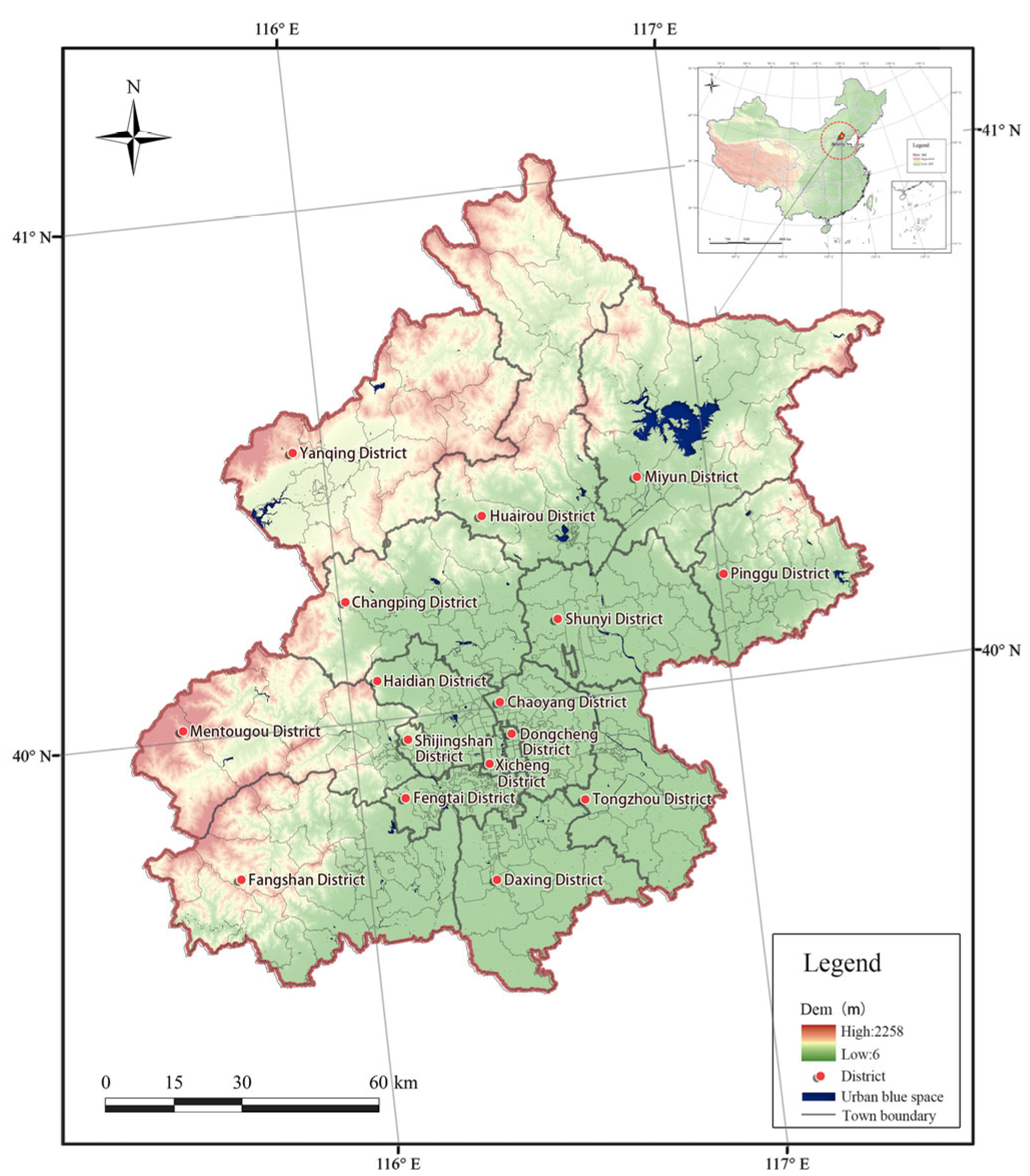
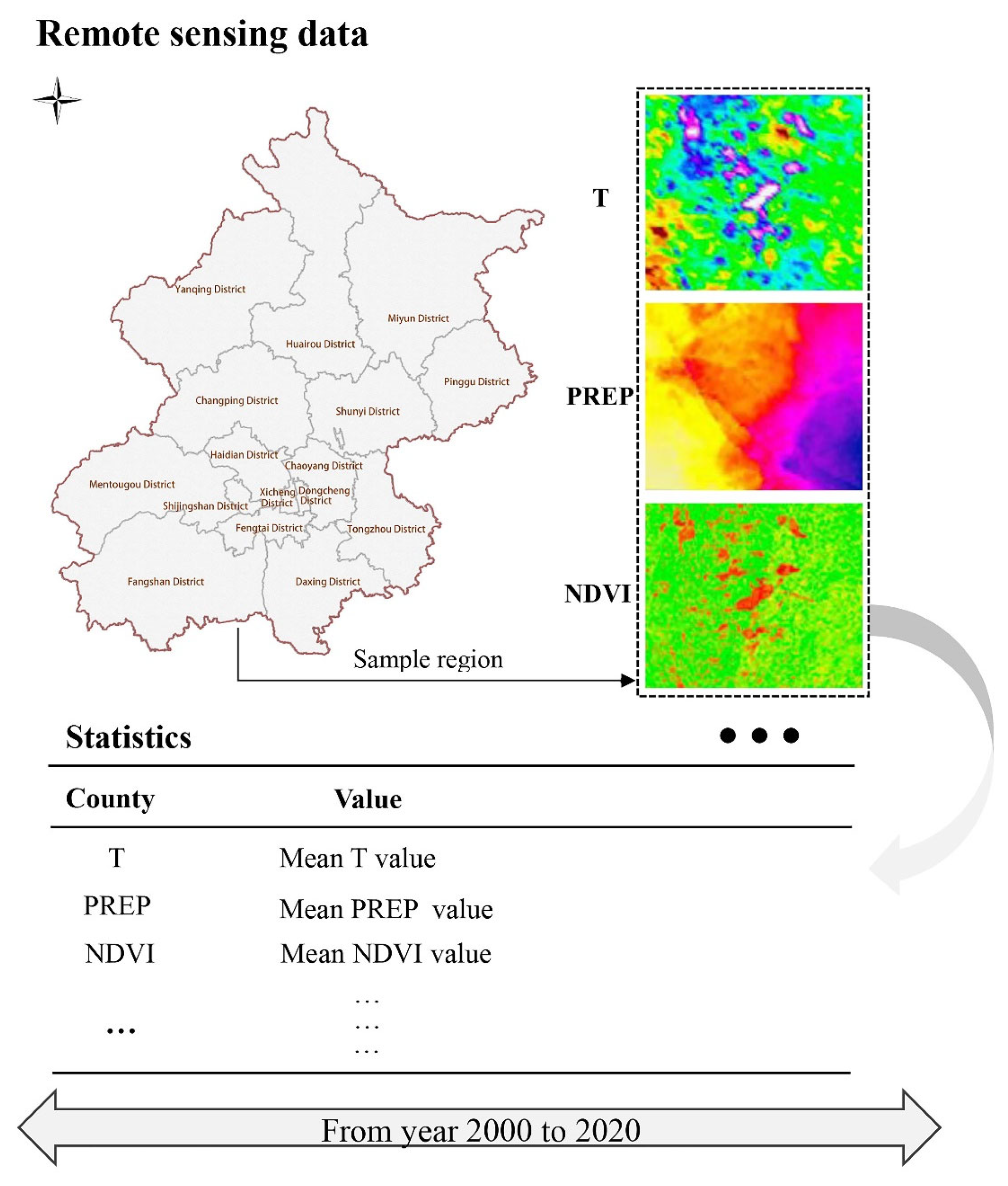
2.1. Study Area

The study area of this research is Beijing, which is a prominent political, economic, and cultural center in China. Beijing is situated between 115.7°E–117.4°E longitude and 39.4°N–41.6°N latitude [48]. It shares borders with Tianjin in the east and Hebei in the remaining directions (see Figure 1). The city covers an area of 16,410 square kilometers, and had a permanent resident population of 21.89 million as of 2021 [49]. Beijing experiences a monsoon-influenced humid continental climate. Summers in Beijing are hot, humid, and prone to rainfall, while winters are cold, dry, and characterized by clear skies. The average annual rainfall in Beijing is approximately 698.4 mm, and the average annual temperature ranges from 9 °C to 19 °C [50].

Beijing serves as a typical case for studying urban blue space (UBS) in a metropolis. The city’s UBS plays a crucial role in several aspects. First, due to the frequent intense rainfall and extreme precipitation events that occur during the summer, UBS serves as a vital component of natural reservoirs, helping to absorb and regulate excess water, thereby reducing the risk of flooding. Additionally, UBS in Beijing provides valuable mental and recreational benefits to the public. As a special urban landscape, UBS is a source of mental relaxation and entertainment for the city’s residents amidst their fast-paced lives. These blue spaces create a serene and tranquil environment, offering an escape from the hustle and bustle of urban life. The presence of UBS in Beijing contributes to the overall well-being and quality of life for its inhabitants. Considering the dual functions of flood mitigation and mental well-being, studying UBS in Beijing provides valuable insights into the multifaceted role of blue spaces in metropolises.

2.2. Data and Resources

We chose Beijing as the study area to explore the spatial and temporal characteristics and the mechanisms of urban blue space. Firstly, we used the remote sensing dataset JRC Monthly Water History to extract urban blue space, described the area development from 2000 to 2020, scheduled Moran’s I to analyze the spatial autocorrelation, and used Getis-Ord General G* to reveal the spatial clustering pattern. Secondly, using Fragstats 4.2, we calculated ten landscape indexes and extracted the main aspects of those indexes by PCA. Thirdly, we used grey relation analysis to simulate the mechanisms of the UBS area and landscapes, then classified the main influencing factors as strong, medium, and weak using the natural break method (Figure 2).

Remote sensing images from the Google Earth engine data catalog were used to extract influencing factors. The statistical data were retrieved from the statistical yearbook and official websites (

Table 1. Data and resources.

Number	Name	Dataset	Spatial Resolution	Temporal Resolution
1	POP	Gridded Population of the World, Version 4	100 m	Yearly
2	PREP	ERA5-Land	0.1 × 0.1	Daily
3	T	Aqua/Terra MODIS MYD11A2	1000 m	Eight days
4	FVC	MODIS MCD12Q1	500 m	Yearly
5	ASP	MODIS MCD12Q1	500 m	Yearly
6	NDVI	MODIS NDVI MYD13Q1 V6	250 m	Sixteen days
7	EVI	MODIS NDVI MYD13Q1 V6	250 m	Sixteen days
8	GDP	Beijing Statistical Yearbook; Beijing Statistical Bulletin of National Economic and Social Development	_	Yearly
9	UEM	Beijing and each districts statistical yearbook	_	Yearly
10	EDUI	Beijing and each districts statistical yearbook	_	Yearly
11	STI	Beijing and each districts statistical yearbook	_	Yearly
12	UBS	JRC Monthly Water History, v1.3	30 m	Monthly

).

To address the spatial and temporal resolution differences between remote sensing images and statistical data, the influencing factors derived from remote sensing images were aggregated to the county level from the pixel scale. This aggregation process ensures that the data align with the resolution of the statistical data available. Furthermore, to account for the temporal variations within the remote sensing images, the data were further derived to annual averages. This averaging process provides a representative value for each influencing factor, smoothing out short-term fluctuations and capturing the overall trends over time. By aggregating and deriving the data, this study ensures compatibility and consistency between the remote sensing images and the available statistical data, enabling a comprehensive and integrated analysis of the influencing factors at the district level on an annual basis (Figure 3).

We used multi-resource data, including remote sensing and statistics data with different spatio-temporal resolutions. We extracted the annual average at the county scale to unify the temporal and spatial scales of all data.

Referring to the existing research, considering the actual situation and data availability in Beijing, we have selected the following indicators as influencing factors for studying UBS.

Population (POP): Population is a critical factor influencing UBS scope and intensity [51,52]. Domestic water consumption and modifications to surface runoff by human activities significantly impact UBS. Therefore, population is a relevant indicator in this study.

Precipitation (PREP): Urban precipitation plays a vital role in the groundwater recharge and overall water circulation in cities. Extreme weather events associated with global climate change can generate temporary urban blue spaces, such as groundwater puddles. Hence, precipitation is commonly considered an influential indicator in UBS research [53].

Temperature (T): UBS and temperature represent a complex system interaction. UBS helps regulate the local microclimate, mitigating high temperatures and providing substantial cooling effects to the surrounding areas [54]. Higher temperature accelerates waterbody shrinking through increased evaporation. Thus, temperature is a significant factor to consider in UBS studies [55].

Fractional vegetation cover (FVC): Vegetation plays a crucial role in slowing surface runoff and enhancing water conservation capacity [56,57]. Considering the positive influence of vegetation on UBS, FVC is an essential indicator in this study.

Artificial surface proportion (ASP): The proportion of artificial surface in a city significantly affects its surface temperature, leading to either warming or cooling effects. Analyzing ASP helps in understanding urban ecological health and the impact of ASP on UBS [58].

Normalized difference vegetation index: NDVI is closely associated with the cooling effect of urban ecological spaces and precipitation [59]. It is more sensitive than the enhanced vegetation index (EVI) in regions with sparse vegetation, which are often found in metropolises such as Beijing. Thus, NDVI is a suitable indicator for UBS research in Beijing.

Enhanced vegetation index (EVI): EVI is a robust remote sensing index that reflects vegetation density and is especially effective for dense vegetation surfaces. It is closely related to urban microcirculation and blue spaces [60].

Gross domestic product (GDP): GDP measures the gross product of a country and indirectly reflects water consumption, wastewater discharge, and water-use efficiency [61,62]. Considering the implications for water management and efficiency, GDP is a relevant indicator in this study.

Urban environmental management (UEM): UEM encompasses water conservancy, public facilities, and land use planning to ensure that population growth is in alignment with access to natural resources, basic infrastructure, and shelter. UEM encompasses the water management sector, flood control facilities management, water resources management, natural water collection and distribution, as well as hydrological services. It also includes the ecological protection and environmental governance industry, covering aspects such as ecological protection and environmental governance. Additionally, UEM involves public facilities management, which comprises municipal facilities management, environmental health management, urban and rural appearance management, and greening management.

Educational investment (EDUI): Education investment significantly promotes science and technology, which in turn affects production methods and water consumption efficiency. It is closely related to UBS and its sustainability.

Scientific and technical investment (STI): STI drives the application of technologies such as the Internet of Things (IoT), YunOS IoT, and big data. These technologies optimize water consumption patterns and UBS planning, making STI a relevant indicator in understanding UBS dynamics.

2.3. Methodology

2.3.1. Spatial Autocorrelation Analysis and Spatial Clustering Analysis

Spatial autocorrelation detects the convergence or dispersion of observations [63,64]. $\mathrm{M}\mathrm{o}\mathrm{r}\mathrm{a}\mathrm{n}’\mathrm{s} I$ is a widely used classical spatial autocorrelation index. For a series of n variable samples, $x_i$ is the observation at location i, and w_ij is the spatial weight matrix (SWM). Then, $\mathrm{M}\mathrm{o}\mathrm{r}\mathrm{a}\mathrm{n}’\mathrm{s} I$ is calculated as follows:

$$I=\frac{n{\sum }_{i=1}^n{\sum }_{j=1}^n{w}_{ij}(x_i-\overline{x})(x_j-\overline{x})}{{\sum }_{i=1}^n{\sum }_{j=1}^n{w}_{ij}{\sum }_{i=1}^n{(x_i-\overline{x})}^2}$$

$\mathrm{M}\mathrm{o}\mathrm{r}\mathrm{a}\mathrm{n}’\mathrm{s} I$ ranges from −1 to 1. $\mathrm{M}\mathrm{o}\mathrm{r}\mathrm{a}\mathrm{n}’\mathrm{s}$ $I$ > 0 indicates a positive spatial correlation. The closer it is to 1, the more significant the positive spatial autocorrelation. $\mathrm{M}\mathrm{o}\mathrm{r}\mathrm{a}\mathrm{n}’\mathrm{s} I$ < 0 indicates a negative spatial correlation. The closer it is to −1, the more significant the negative spatial autocorrelation. $\mathrm{M}\mathrm{o}\mathrm{r}\mathrm{a}\mathrm{n}’\mathrm{s} I$ = 0 indicates a random distribution [65]. The high/low clustering (Getis-Ord General G*) tool is an effective method for spatial aggregation simulation. The calculation formula is as follows:

$$\mathrm{G}*=\frac{{\sum }_{j=1}^n{w}_{ij}{x}_j-\overline{x}{\sum }_{j=1}^n{w}_{ij}}{\sqrt{\frac{{\sum }_{j=1}^n{x}_j^2}{n}-\frac{1}{x^2}}\sqrt{\frac{\left[{n{\sum }_{j=1}^n{w}_{ij}^w-\left({\sum }_{j=1}^n{w}_{ij}\right)}^2\right]}{n-1}}}$$

$\overline{x}$ is the average of observations, $x_1,x_2,\dots ,x_n { w}_{ij}$ is the spatial weight of $x_i$, and $x_j$, $i,j=\mathrm{1,2},\dots ,$n. The higher G* is, the higher the observation clustering, and vice versa. The null hypothesis of General G* assumes that the observations do not cluster spatially [66]. The p value determines whether the null hypothesis should be accepted or not. The z score reflects the dispersion of observations [67].

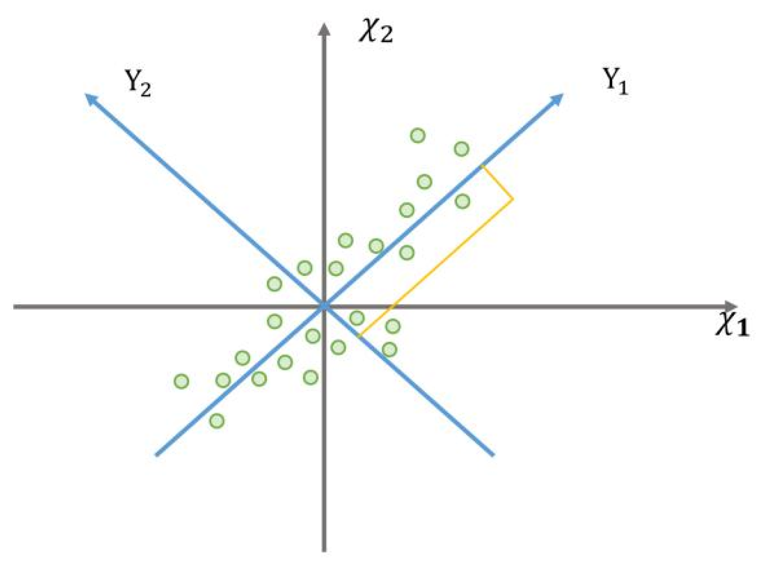
2.3.2. Principal Components Regression Analysis

Principal component regression analysis (PCR) is used to solve multivariate collinearity problems [68]. Principal component analysis, or PCA, is a dimensionality reduction method that is often used to reduce the dimensionality of large data sets by transforming a large set of variables into a smaller one that still contains most of the information in the large set. Principal component analysis (PCA) converts multiple indexes into several comprehensive indexes by orthogonal rotation transformation, following the premise of minimizing information loss. Generally, the results of PCA are independent variables called principal components [69]. The geometric interpretation and model of PCA are as follows (Figure 4):

The distribution of a series of n binary observations ($x_{11}, x_{12}, \dots , x_{n1},x_{n2})$ in the coordinate space composed of $X_1$ and $X_2$ is shown in Figure 4. Along the $X_1$ or $X_2$ axis, observation points have large discretization indicated by the variance of $X_1$ or $X_2$, respectively. Axes $X_1$ and $X_2$ are rotated counterclockwise to axes $Y_1$ and $Y_2$ following formula X. The dispersion of n observation points on the $Y_1$ axis is the largest, indicating that variable $Y_1$ retains most of the information of the original data.

$$\left(\begin{array}{c}{Y}_1\\ Y_2\end{array}\right)=\left(\begin{array}{c}\mathit{cos}\theta \mathit{sin}\theta \\ -\mathit{sin}\theta \mathit{cos}\theta \end{array}\right)\left(\begin{array}{c}{X}_1\\ X_2\end{array}\right)=UX$$

2.3.3. Grey Relation Analysis

A complex system always involves various elements; the mechanism of each element is hard to simulate quantitively in practice because of the associated interactions. Grey system theory attempts to look for quantitative relationships based on the curve geometry [70,71,72]. Sequences are closely related when they have tight geometry curves and similar trends, and vice versa. Thus, grey correlation analysis is an effective classical quantitative measure for dynamic series. The formula is as follows:

$$r\left(x_0\left(k\right),x_i\left(k\right)\right)=\frac{\underset{i}{\min }\underset{k}{\min }\left|x_0\left(k\right)-x_i\left(k\right)\right|+\xi \underset{i}{\max }\underset{k}{\max }\left|x_0\left(k\right)-x_i\left(k\right)\right|}{\left|x_0\left(k\right)-x_i\left(k\right)\right|+\xi \underset{i}{\max }\underset{k}{\max }\left|x_0\left(k\right)-x_i\left(k\right)\right|}$$

$$r\left(x_0,x_i\right)=\frac{1}{n}\sum _{k=1}^{n}r(x_0\left(k\right),x_i(k\left)\right)$$

where $r\left(x_0\left(k\right),x_i\left(k\right)\right)$ is the grey correlation coefficient at location $k$, and $x_0$ and $x_i$ are the observations of data sequences $X_0$ and $X_1$, respectively. $\xi$ refers to the resolution coefficient. The value of $\xi$ is inversely proportional to the difference between sequence phases. In classical statistical theory, for a set of observations with a large sample size, the probability of the sample is approximately equal to the frequency. Thus, $\xi$ is equal to 0.5.

3. Results

3.1. Spatiotemporal Analysis of Blue Space Area

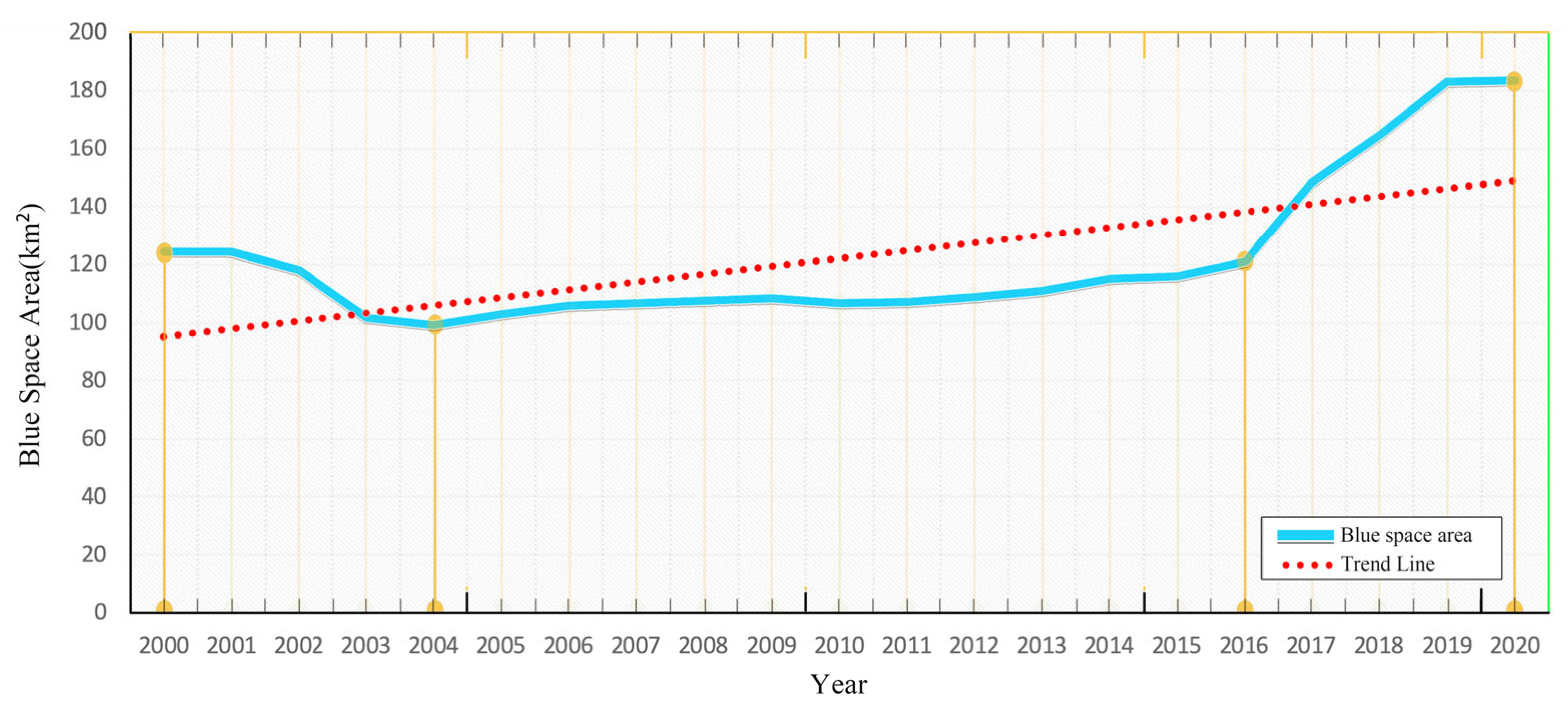
3.1.1. Development Characteristics of the UBS Area in Beijing

The UBS area (S) in Beijing showed a slight increasing trend from 2000 to 2020, with a stable trend from 2004 to 2016. It has been clearly increasing since 2016. The area of UBS in Beijing was 124.4 km² in 2000, reducing to 99.08 km² in 2004, rising slightly to 121 km² in 2016, and increasing to 183.4 km² in the last four years (Figure 5).

3.1.2. Spatial Autocorrelation Analysis of the UBS in Beijing

Considering a confidence level of α = 0.05, Moran’s I is always lower than 0.2, which indicates the weak spatial autocorrelation of the UBS in Beijing.

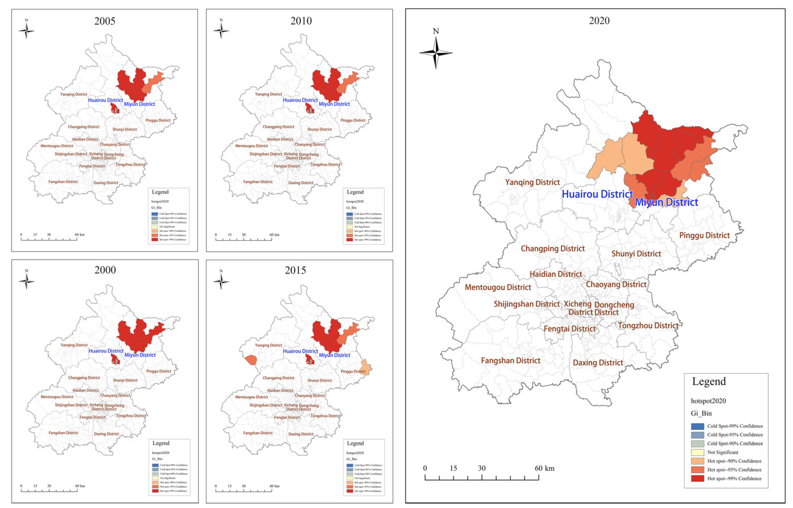
3.1.3. Spatial Clustering Pattern of the UBS in Beijing

From 2000 to 2020, the cluster analysis of “high/low” revealed that the agglomeration characteristics of UBS were relatively stable at the county level. However, the significance of clustering in Tai Shitun decreased prominently (Figure 6).

3.2. Spatiotemporal Analysis of the UBS Landscape in Beijing

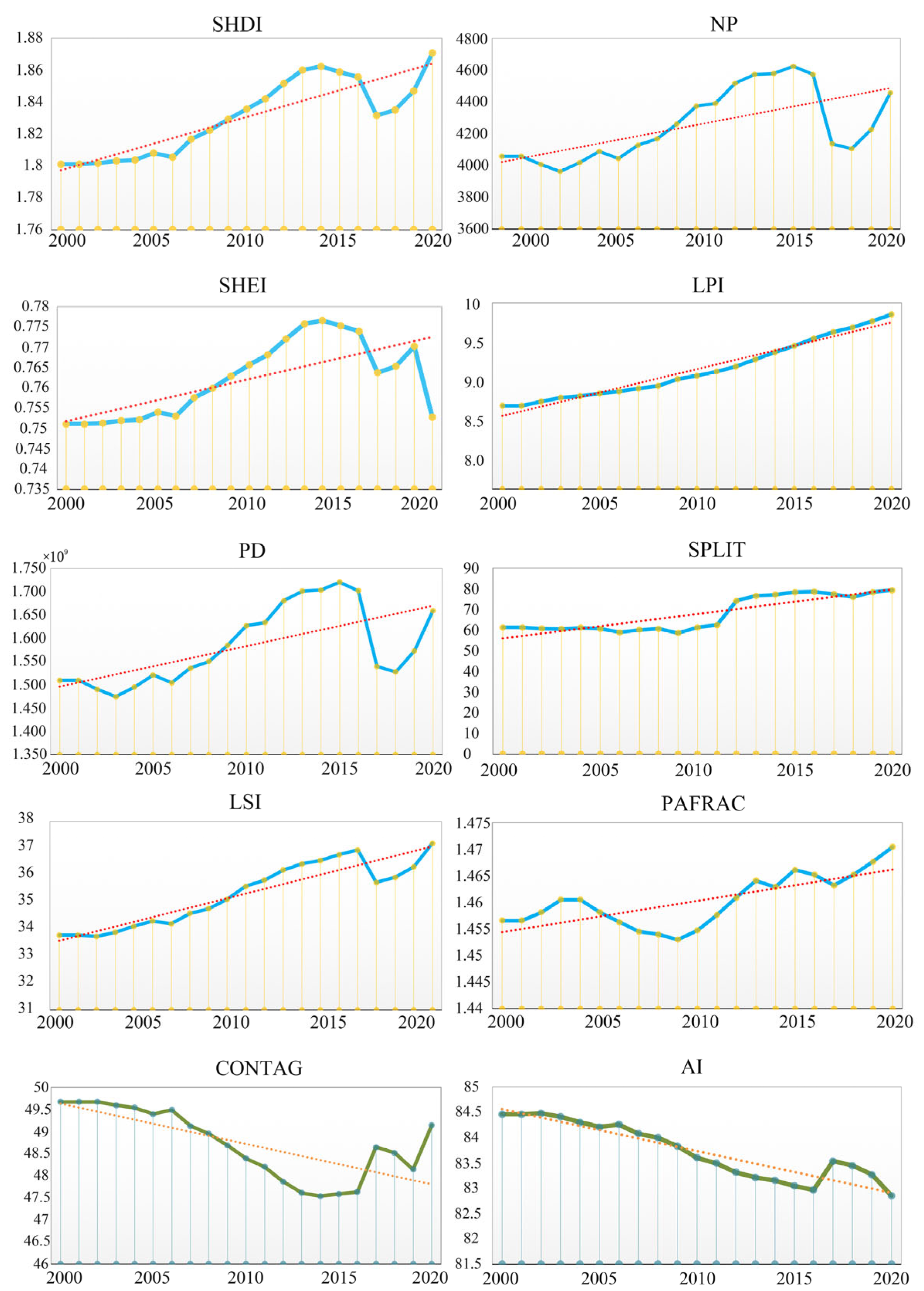
3.2.1. Analysis of Landscape Indicators

The landscape pattern comprehensively reflects landscape spatial heterogeneity. Patterns reveal the spatial distribution and combination of different patches. These patches are always of various sizes, shapes, and attributes.

In this study, multiple landscape indexes were computed. Specific indicators included LPI, SPLIT, CONTAG, AI, PD, NP, LSI, SHDI, SHEI, and PAFRAC. The detailed descriptions and formulas of these indicators are presented in

Table 2. Landscape indexes.

LPI (Largest Patch Index)	Area Percentage of Maximum Patch
SPLIT (Splitting index)	Dispersion among different patches at a landscape scale. The higher the value of SPLIT, the more separation between studied patch types.
CONTAG (Contagion index)	Spatial collection and decentralization. The smaller the value of CONTAG, the sparser each patch type.
AI (Aggregation index)	Connectivity between patches of all patch types. The lower the value is, the more discrete the landscape.
PD (Patch density)	Patch density in the landscape reflects the degree and type of landscape fragmentation. Patch density represents the spatial heterogeneity of the landscape per unit area.
NP (Number of patches)	Number of all patches distributed in the landscape.
LSI (Landscape shape index)	Indicates the change in landscape form. The higher the value, the more complex the shape.
SHDI (Shannon’s diversity index)	Reflects how many different quantitative measures are in a dataset.
SHEI (Shannon’s evenness index)	Describes the extent of the landscape controlled by minority patch types.
PAFRAC (Perimeter area fractal dimension)	The intensity index reflects the disturbance in landscape patterns due to human activities. The higher the value, the greater the landscape’s external disturbance.

[73].

The elements with upward trends are LPI, SPLIT, PD, NP, LSI, SHDI, SHEI, and PAFRAC (Figure 7). Their changes show that the UBS landscape pattern in Beijing developed stably in the first two decades. The maximum landscape patch area is increasing. Patches are more complex and have a significant change in intensity. Diversity and richness are improved. The patches are distributed more evenly. Landscape patch types have become more diverse because of human effects. As a result, the extent of separation, fragmentation, and spatial heterogeneity indexes was more remarkable and higher.

The indicators with downward trends are AI and CONTAG (Figure 7). In the last 21 years, the landscape connectivity of UBS in Beijing has been shallow, and the downward trend was kept up with the sprawl of urban construction.

3.2.2. Principal Component Analysis of the UBS Spatial Landscape Indices

The cumulative contribution rate of the first two principal components (Z₁ and Z₂) is 93.9% (

Table 3. Results of principal component analysis.

Component	Eigenvalue	Contribution Rate	Cumulative Contribution Rate
1	8.162	81.623	81.623
2	1.228	12.280	93.903
3	0.328	3.276	97.179
4	0.222	2.224	99.403
5	0.043	0.427	99.830
6	0.014	0.140	99.970
7	0.003	0.029	99.999
8	0.000	0.001	100.000
9	0.000	0.000	100.000
10	0.000	0.000	100.000

), indicating that the first two principal components contain 93.9% of the information of the 10 original components. Thus, the landscape indexes of the UBS could be significantly extracted to the two component indicators (Formula 1, 2). Using principal component loadings, we can calculate UBS landscape index (Z).

Z1 = 0.925NP + 0.925PD + 0.384LPI + 0.735LSI + 0.156PAFRAC − 0.913CONTAG + 0.456SPLIT + 0.784SHDI + 0.895SHEI − 0.736AI

(1)

Z2 = 0.295NP + 0.295NP + 0.881LPI + 0.66LSI + 0.946PAFRAC − 0.32CONTAG + 0.855SPLIT + 0.587SHDI + 0.273SHEI − 0.659AI

(2)

Z = 0.8162Z1 + 0.1228Z2

(3)

Z₁ is highly positively related to NP, PD, and SHEI, and is negatively related to CONTAG, indicating a spatial distribution structure at a landscape scale. According to formula (1), NP, PD, CON, and SHEI contribute to Z₁ significantly, with coefficients greater than 0.8, referring to the fact that Z₁ is closely related to the integrality of the landscape. The higher the Z₁, the greater the NP, PD, and SHEI indexes, and the smaller the CONTAG value, indicating more patches; the higher the patch density, the lower the agglomeration degree of various patches. Z₂ is positively related to PAFRAC, LPI, and SPLIT, reflecting the spatial distribution structure at the patch scale. According to formula (2), PAFRAC, LPI, and SPLIT contribute to Z₂ significantly, with coefficients greater than 0.8, referring to the fact that Z₂ is closely related to the malconformation of the landscape. The higher the Z₂, the greater the PAFRAC, LPI, and SPLIT indexes, meaning a more complex patch shape, a more extensive patch area, and a greater distance between patches. Z is the UBS landscape index. The greater Z is, the larger Z₁ and Z₂ are, representing a greater NP, PD, SHEI, SHDI, PAFRAC, LPI, SPLIT, and LSI, and a smaller CONTAG and AI, reflecting more severe UBS fragmentation and weaker spatial aggregation.

Z₁ increased steadily from 2000 to 2014 and decreased until 2020, with a downward trend overall. The results revealed that the UBS patch number, density, and diversity had increased at fourteen years, and then declined in the last six years; the agglomeration weakened and then decreased. Overall, UBS in Beijing has faced severe fragmentation, which is expected to slow in recent years.

In contrast, Z₂ decreased in the first decade and increased in the second decade, trending upward. The results showed that the shape complexity, area, and distance decreased first and then increased. From the perspective of the whole period, UBS in Beijing was disturbed from 2000 to 2020, and has been declining in the last decade.

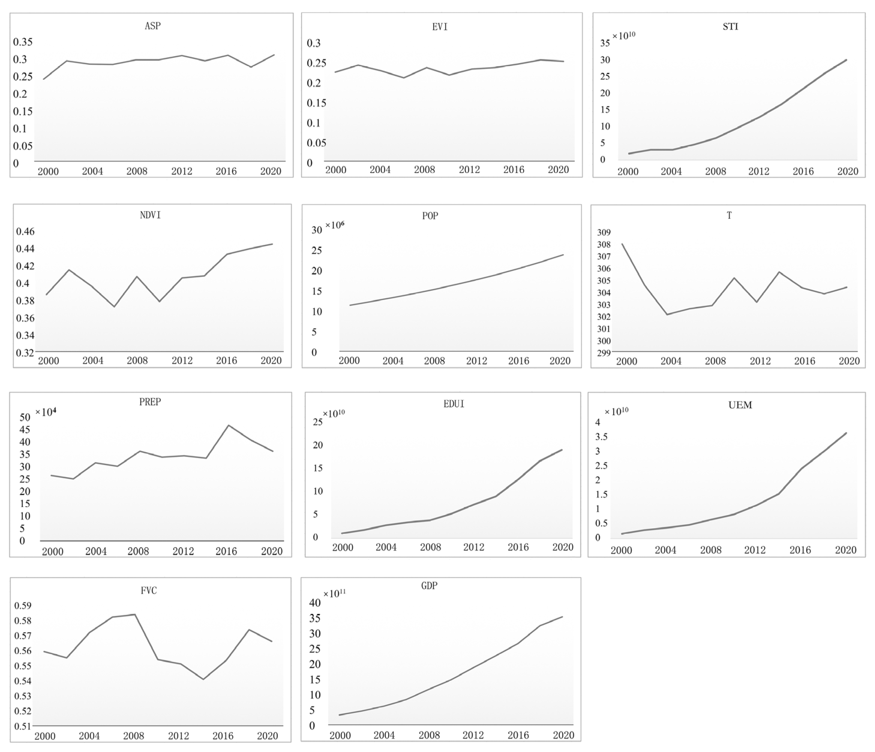
3.3. Mechanisms Driving the Area of UBS

According to the correlation coefficients, the influencing factors rated from most to least importance are as follows: UEM > EDUI > STI > NDVI > T > GDP > POP > FVC > EVI > PREP > ASP.

The influencing factors were identified as strong factors (UEM, EDUI, STI), medium factors (NDVI, T, GDP, POP), and weak factors (FVC, EVI, PREP, ASP) according to the Jenks Natural Breaks Classification.

The results showed that scientific technology factors greatly influenced the UBS area, with correlation coefficients greater than 0.7. The strongest factor is UEM, with the highest coefficient of 0.798, followed by EDUI and STI, with coefficients of 0.759 and 0.758, respectively. The coefficients of NDVI and EVI indicated that the sparse vegetation surface magnified the UBS area more than the dense vegetation surface. POP and GDP have influenced UBS area, with correlation coefficients of 0.68 and 0.689, respectively. With correlation coefficients of 0.5, the influence of ASP on UBS area is smaller than that of natural and technology factors FVC and PREP.

3.4. Mechanisms Influencing the UBS Landscape

From the perspective of UBS landscapes, the influencing factors were rated as follows: PREP > POP > GDP > STI > T > EDUI > UEM > ASP > NDVI > EVI > FVC (

Table 4. Correlation analysis of UBS area and landscapes.

Influencing Factors	Correlation Coefficients of UBS Area (S)	Correlation Coefficients of UBS Landscapes (Z)
UEM	0.798	0.664
EDUI	0.759	0.665
STI	0.758	0.686
NDVI	0.697	0.617
T	0.692	0.685
GDP	0.689	0.691
POP	0.68	0.692
FVC	0.659	0.493
EVI	0.658	0.585
PREP	0.62	0.732
ASP	0.5	0.656

). According to the results of the Jenks Natural Breaks Classification, the strong factors influencing the UBS landscape are PREP, POP, GDP, STI, and T, the medium factors are EDUI, UEM, and ASP, and the weak factors are NDVI, EVI, and FVC. Thus, it is reasonable to conclude that precipitation and human activities influence the UBS landscape more than vegetation factors.

POP and GDP have a great impact on UBS landscape, with correlation coefficients of 0.692 and 0.691, respectively, following the greatest indicator of 0.732, PREP. Technological factors have influenced the UBS landscape significantly, with correlation coefficients greater than 0.664. ASP is the next, with a correlation coefficient of 0.656. The smallest coefficient is 0.493, indicating that FVC has the weakest impact on UBS landscape.

4. Discussion

Urban blue space is essential to human life, especially for mental health and quality of life, which has caught eyes worldwide [74]. The UBS area initially decreased from 2000 to 2004 due to significant water consumption resulting from population growth and industrial activities, leading to water shortages [75]. However, a series of measures aimed at improving water resources and protecting urban water bodies subsequently led to a steady expansion of the UBS area. The implementation of the South–North Water Diversion Project, which began in late 2014, significantly contributed to the increase in UBS area [76]. The year 2016 stands out in particular, with a sharp increase in UBS area, which can be explained by the significantly greater annual precipitation since 2015 [77] and the changes in water availability and management practices after the South–North Water Diversion Project (Figure 8). These findings align with previous research [78].

The landscape pattern of UBS in Beijing showed stability with increasing diversity, richness, and evenness indexes from 2000 to 2020, indicating the generation of more water bodies with diverse properties and purposes. However, the dispersion and spatial heterogeneity indexes were poor, indicating severe fragmentation potentially caused by urban expansion and the erosion of ecological spaces [79]. Water pollution policies implemented since 2015 have helped improve water microcirculation, leading to a reversal of negative trends in 2017, with decreasing density and diversity indexes and increasing connectivity and aggregation indexes.

The UBS in Beijing appeared to have a weak spatial autocorrelation, potentially influenced by artificial water bodies created in heat-island-reducing projects over the past two decades [80]. Stable UBS clustering patterns were observed, with unique spots identified, such a shrinking clustering in Taishitun County, extinct clustering in Huairou District, and expanded clustering in Miyun District. Regulation policies such as vegetable cultivation, reservoir water network development, and reclaimed water usage are likely related to stable development and clustered expansion. Conversely, decreasing and extinct clusterings could be attributed to disturbances from industrial and agricultural consumption, river channel changes, and artificial water bodies [81].

According to the grey relation analysis results, science and technology management factors such as UEM, EDUI, and STI strongly impact the UBS area, in which UEM is the most vital factor, in accordance with the result of past research. Vaeztavakoli et al. emphasized that urban management is vital to urban blue space [82], while precipitation and human activities strongly influence UBS landscapes. Scientific technologies enhance production efficiency and water utilization efficiency, reducing water consumption and expanding the UBS area.

Precipitation replenishes water storage in urban water bodies and promotes vegetation growth, directly affecting the landscape pattern of the UBS. Human activities, including land use changes and surface modifications, have a direct and significant impact on UBS landscapes. Medium influencing factors, such as sparse vegetation, temperature, economy, and population, have a moderate influence on UBS area and landscapes. Weak factors are associated with land use patterns, particularly in dense vegetation areas, reflecting the limited correlation in these regions [83]. The weak influencing factors in UBS landscapes are closely related to vegetation.

5. Conclusions

We employed remote sensing techniques to extract urban blue space (UBS) in Beijing and conducted a comprehensive analysis of its spatial and temporal development over the past two decades using ESDA methods. From an ecological perspective, we examined a wide range of landscape patterns, including area and composition, and quantitatively simulated the underlying mechanisms. The main findings are as follows: (1) The UBS area in Beijing experienced a decline from 2000 to 2004, followed by a steady increase over the next decade and a significant surge since 2016. (2) The spatial clustering of UBS exhibited overall stability with subtle variations. (3) With the exception of artificial surface proportion (ASP), UBS results in a more than 0.6% change in UBS area for every 1% change in those factors. (4) In terms of UBS area, urban environmental management (UEM), educational investment (EDUI), and scientific and technical investment (STI) were identified as strong influencing factors; normalized difference vegetation index (NDVI), temperature (T), gross domestic product (GDP), and population (POP) were classified as medium influencing factors; fractional vegetation cover (FVC), enhanced vegetation index (EVI), precipitation (PREP), and ASP were considered weak influencing factors. In terms of UBS composition, PREP, POP, GDP, STI, and T were factors; EDUI, urban environmental management (UEM), and ASP were classified as medium influencing factors; NDVI, EVI, and FVC were considered weak influencing factors. (5) Dense vegetation cover and sparse vegetation cover had distinct impacts on UBS area while exhibiting similar effects on UBS landscape patterns.

This study successfully uncovered the spatiotemporal characteristics of the UBS area and landscapes in Beijing from 2000 to 2020 and elucidated the multifactorial mechanisms driving these changes. However, the analysis resolution was limited to counties due to the availability of policy number and statistics data, rather than at the pixel level. Further research is needed to explore UBS at a finer scale. Additionally, while the study analyzed 11 influencing factors, it is acknowledged that there may be other factors that should have been explored, such as the number and effectiveness of policies. Furthermore, due to data limitations, the study focused on a 21-year period, and longer-term research is warranted in the future.

References

1. Ampatzidis, P.; Kershaw, T. A review of the impact of blue space on the urban microclimate. Sci. Total Environ. 2020, 730, 139068. [Google Scholar] [CrossRef] [PubMed]
2. Foley, J.A.; Defries, R.; Asner, G.P.; Barford, C.; Bonan, G.; Carpenter, S.R.; Chapin, F.S.; Coe, M.T.; Daily, G.C.; Gibbs, H.K.; et al. Global consequences of land use. Science 2005, 309, 570–574. [Google Scholar] [CrossRef] [PubMed]
3. Gunawardena, K.R.; Wells, M.J.; Kershaw, T. Utilising green and bluespace to mitigate urban heat Island intensity. Sci. Total Environ. 2017, 584–585, 1040–1055. [Google Scholar] [CrossRef] [PubMed]
4. Perosa, F.; Fanger, S.; Zingraff-Hamed, A.; Disse, M. A meta-analysis of the value of ecosystem services of floodplains for the Danube River Basin. Sci. Total Environ. 2021, 777, 146062. [Google Scholar] [CrossRef] [PubMed]
5. Georgiou, M.; Tieges, Z.; Morison, G.; Smith, N.; Chastin, S. A population-based retrospective study of the modifying effect of urban blue space on the impact of socioeconomic deprivation on mental health, 2009–2018. Sci. Rep. 2022, 12, 13040. [Google Scholar] [CrossRef] [PubMed]
6. Martínez-Arroyo, A.; Jáuregui, E. On the environmental role of urban lakes in Mexico city. Urban Ecosyst. 2000, 4, 145–166. [Google Scholar] [CrossRef]
7. He, B.J.; Zhu, J.; Zhao, D.; Gou, Z.H.; Qi, J.D.; Wang, J. Co-benefits approach: Opportunities for implementing sponge city and urban heat island mitigation. Land Use Policy 2019, 86, 147–157. [Google Scholar] [CrossRef]
8. Adams, K.D.; Sada, D.W. Surface water hydrology and geomorphic characterization of a playa lake system: Implications for monitoring the effects of climate change. J. Hydrol. 2014, 510, 92–102. [Google Scholar] [CrossRef]
9. Joosse, S.; Hensle, L.; Boonstra, W.J.; Ponzelar, C.; Olsson, J. Fishing in the city for food—A paradigmatic case of sustainability in urban blue space. NPJ Urban Sustain. 2021, 1, 41. [Google Scholar] [CrossRef]
10. Anderson, E.P.; Jackson, S.; Tharme, R.E.; Douglas, M.; Flotemersch, J.E.; Zwarteveen, M.; Lokgariwar, C.; Montoya, M.; Wali, A.; Tipa, G.T.; et al. Understanding rivers and their social relations: A critical step to advance environmental water management. WIREs Water 2019, 6, e1381. [Google Scholar] [CrossRef]
11. Chang, N.; Luo, L.; Wang, X.C.; Song, J.; Han, J.; Ao, D. A novel index for assessing the water quality of urban landscape lakes based on water transparency. Sci. Total Environ. 2020, 735, 139351. [Google Scholar] [CrossRef]
12. Yu, H.; Song, Y.; Chang, X.; Gao, H.; Peng, J. A scheme for a sustainable urban water environmental system during the urbanization process in China. Engineering 2018, 4, 190–193. [Google Scholar] [CrossRef]
13. Coutts, A.M.; Tapper, N.J.; Beringer, J.; Loughnan, M.; Demuzere, M. Watering our cities: The capacity for water sensitive urban design to support urban cooling and improve human thermal comfort in the Australian context. Prog. Phys. Geogr. Earth Environ. 2013, 37, 2–28. [Google Scholar] [CrossRef]
14. Völker, S.; Kistemann, T. Developing the urban blue: Comparative health responses to blue and green urban open spaces in Germany. Health Place 2015, 35, 196–205. [Google Scholar] [CrossRef]
15. Wang, M.; Du, L.; Ke, Y.; Huang, M.; Zhang, J.; Zhao, Y.; Li, X.; Gong, H. Impact of climate variabilities and human activities on surface water extents in reservoirs of Yongding River Basin, China, from 1985 to 2016 based on landsat observations and time series analysis. Remote Sens. 2019, 11, 560. [Google Scholar] [CrossRef]
16. Liu, L.; Fryd, O.; Zhang, S. Blue-green infrastructure for sustainable urban stormwater management—Lessons from six municipality-led pilot projects in Beijing and Copenhagen. Water 2019, 11, 2024. [Google Scholar] [CrossRef]
17. Huang, H.; Yang, H.; Chen, Y.; Chen, T.; Bai, L.; Peng, Z.R. Urban green space optimization based on a climate health risk appraisal—A case study of Beijing city, China. Urban For. Urban Green. 2021, 62, 127154. [Google Scholar] [CrossRef]
18. Helbich, M.; Yao, Y.; Liu, Y.; Zhang, J.; Liu, P.; Wang, R. Using deep learning to examine street view green and blue spaces and their associations with geriatric depression in Beijing, China. Environ. Int. 2019, 126, 107–117. [Google Scholar] [CrossRef]
19. Dou, Y.; Zhen, L.; De Groot, R.; Du, B.; Yu, X. Assessing the importance of cultural ecosystem services in urban areas of Beijing municipality. Ecosyst. Serv. 2017, 24, 79–90. [Google Scholar] [CrossRef]
20. Gašparović, S.; Sopina, A.; Zeneral, A. Impacts of Zagreb’s urban development on dynamic changes in stream landscapes from mid-twentieth century. Land 2022, 11, 692. [Google Scholar] [CrossRef]
21. Hysa, A. Introducing transversal connectivity index (TCI) as a method to evaluate the effectiveness of the blue-green infrastructure at metropolitan scale. Ecol. Indic. 2021, 124, 107432. [Google Scholar] [CrossRef]
22. Luo, S.; Xie, J.; Furuya, K. Assessing the preference and restorative potential of urban park blue space. Land 2021, 10, 1233. [Google Scholar] [CrossRef]
23. Zhao, J.; Guo, W.; Huang, W.; Huang, L.; Zhang, D.; Yang, H.; Yuan, L. Characterizing spatiotemporal dynamics of land cover with multi-temporal remotely sensed imagery in Beijing during 1978–2010. Arab. J. Geosci. 2014, 7, 3945–3959. [Google Scholar] [CrossRef]
24. Wu, J.; Yang, S.; Zhang, X. Interaction analysis of urban blue-green space and built-up area based on coupling model—A case study of Wuhan central city. Water 2020, 12, 2185. [Google Scholar] [CrossRef]
25. Wang, S.; Yang, K.; Yuan, D.; Yu, K.; Su, Y. Temporal-spatial changes about the landscape pattern of water system and their relationship with food and energy in a mega city in China. Ecol. Model. 2019, 401, 75–84. [Google Scholar] [CrossRef]
26. Cao, H.; Liu, J.; Chen, J.; Gao, J.; Wang, G.; Zhang, W. Spatiotemporal patterns of urban land use change in typical cities in the greater mekong subregion (GMS). Remote Sens. 2019, 11, 801. [Google Scholar] [CrossRef]
27. Xie, Y.; Wang, G.; Wang, X.; Fan, P. Assessing the evolution of oases in arid regions by reconstructing their historic spatio-temporal distribution: A case study of the Heihe River Basin, China. Front. Earth Sci. 2017, 11, 629–642. [Google Scholar] [CrossRef]
28. Song, S.; Wang, S.; Shi, M.; Hu, S.; Xu, D. Urban blue–green space landscape ecological health assessment based on the integration of pattern, process, function and sustainability. Sci. Rep. 2022, 12, 7707. [Google Scholar] [CrossRef] [PubMed]
29. Liu, Y.; Zhang, D.; He, K.; Gao, Q.; Qin, F. Research on land use change and ecological environment effect based on remote sensing sensor technology. J. Sens. 2021, 2021, 4351733. [Google Scholar] [CrossRef]
30. Hurford, A.P.; Parker, D.J.; Priest, S.J.; Lumbroso, D.M. Validating the return period of rainfall thresholds used for extreme rainfall alerts by linking rainfall intensities with observed surface water flood events. J. Flood Risk Manag. 2012, 5, 134–142. [Google Scholar] [CrossRef]
31. Brinkmann, K.; Hoffmann, E.; Buerkert, A. Spatial and temporal dynamics of urban wetlands in an Indian megacity over the past 50 years. Remote Sens. 2020, 12, 662. [Google Scholar] [CrossRef]
32. Suligowski, R.; Ciupa, T.; Cudny, W. Quantity assessment of urban green, blue, and grey spaces in Poland. Urban For. Urban Green. 2021, 64, 127276. [Google Scholar] [CrossRef]
33. Steele, M.K.; Heffernan, J.B. Morphological characteristics of urban water bodies: Mechanisms of change and implications for ecosystem function. Ecol. Appl. 2014, 24, 1070–1084. [Google Scholar] [CrossRef] [PubMed]
34. Elmore, A.J.; Kaushal, S.S. Disappearing headwaters: Patterns of stream burial due to urbanization. Front. Ecol. Environ. 2008, 6, 308–312. [Google Scholar] [CrossRef] [PubMed]
35. Brans, K.I.; Engelen, J.M.T.; Souffreau, C.; De Meester, L. Urban hot-tubs: Local urbanization has profound effects on average and extreme temperatures in ponds. Landsc. Urban Plan. 2018, 176, 22–29. [Google Scholar] [CrossRef]
36. Peng, J.; Liu, Q.; Xu, Z.; Lyu, D.; Du, Y.; Qiao, R.; Wu, J. How to effectively mitigate urban heat island effect? A perspective of waterbody patch size threshold. Landsc. Urban Plan. 2020, 202, 103873. [Google Scholar] [CrossRef]
37. Holder, C.D.; Gibbes, C. Influence of leaf and canopy characteristics on rainfall interception and urban hydrology. Hydrol. Sci. J. 2017, 62, 182–190. [Google Scholar] [CrossRef]
38. Walsh, C.J.; Roy, A.H.; Feminella, J.W.; Cottingham, P.D.; Groffman, P.M.; Morgan, R.P. The urban stream syndrome: Current knowledge and the search for a cure. J. N. Am. Benthol. Soc. 2005, 24, 706–723. [Google Scholar] [CrossRef]
39. Pan, H.; Deal, B.; Destouni, G.; Zhang, Y.; Kalantari, Z. Sociohydrology modeling for complex urban environments in support of integrated land and water resource management practices. Land Degrad. Dev. 2018, 29, 3639–3652. [Google Scholar] [CrossRef]
40. Clare, S.; Krogman, N.; Foote, L.; Lemphers, N. Where is the avoidance in the implementation of wetland law and policy? Wetl. Ecol. Manag. 2011, 19, 165–182. [Google Scholar] [CrossRef]
41. Leigh, N.G.; Lee, H. Sustainable and resilient urban water systems: The role of decentralization and planning. Sustainability 2019, 11, 918. [Google Scholar] [CrossRef]
42. Ianoş, I.; Sorensen, A.; Merciu, C. Incoherence of urban planning policy in Bucharest: Its potential for land use conflict. Land Use Policy 2017, 60, 101–112. [Google Scholar] [CrossRef]
43. Jiang, T.T.; Pan, J.F.; Pu, X.M.; Wang, B.; Pan, J.J. Current status of coastal wetlands in China: Degradation, restoration, and future management. Estuar. Coast. Shelf Sci. 2015, 164, 265–275. [Google Scholar] [CrossRef]
44. Völker, S.; Kistemann, T. The impact of blue space on human health and well-being—Salutogenetic health effects of inland surface waters: A review. Int. J. Hyg. Environ. Health 2011, 214, 449–460. [Google Scholar] [CrossRef] [PubMed]
45. Pandey, C.L. Managing urban water security: Challenges and prospects in Nepal. Environ. Dev. Sustain. 2021, 23, 241–257. [Google Scholar] [CrossRef]
46. Zhong, Q.; Ma, J.; Zhao, B.; Wang, X.; Zong, J.; Xiao, X. Assessing spatial-temporal dynamics of urban expansion, vegetation greenness and photosynthesis in megacity Shanghai, China during 2000–2016. Remote Sens. Environ. 2019, 233, 111374. [Google Scholar] [CrossRef]
47. Karmaoui, A.; Ben Salem, A.; El Jaafari, S.; Chaachouay, H.; Moumane, A.; Hajji, L. Exploring the land use and land cover change in the period 2005–2020 in the province of Errachidia, the pre-sahara of Morocco. Front. Earth Sci. 2022, 10, 962097. [Google Scholar] [CrossRef]
48. Investing General Situation of Beijing. Available online: http://www.beijing.gov.cn/renwen/bjgk/ (accessed on 4 April 2023).
49. The People’s Government of Beijing Municipality. Beijing 2021 Statistical Bulletin on National Economic and Social Development. Available online: https://www.beijing.gov.cn/gongkai/shuju/tjgb/202203/t20220301_2618806.html (accessed on 1 March 2022).
50. Peel, M.C.; Finlayson, B.L.; McMahon, T.A. Updated world map of the Köppen-Geiger climate classification. Hydrol. Earth Syst. Sci. 2007, 11, 1633–1644. [Google Scholar] [CrossRef]
51. Raymond, C.M.; Gottwald, S.; Kuoppa, J.; Kyttä, M. Integrating multiple elements of environmental justice into urban blue space planning using public participation geographic information systems. Landsc. Urban Plan. 2016, 153, 198–208. [Google Scholar] [CrossRef]
52. Bedla, D.; Halecki, W. The value of river valleys for restoring landscape features and the continuity of urban ecosystem functions—A review. Ecol. Indic. 2021, 129, 107871. [Google Scholar] [CrossRef]
53. Avashia, V.; Garg, A. Implications of land use transitions and climate change on local flooding in urban areas: An assessment of 42 Indian cities. Land Use Policy 2020, 95, 104571. [Google Scholar] [CrossRef]
54. Dai, X.; Wang, L.; Tao, M.; Huang, C.; Sun, J.; Wang, S. Assessing the ecological balance between supply and demand of blue-green infrastructure. J. Environ. Manag. 2021, 288, 112454. [Google Scholar] [CrossRef] [PubMed]
55. Yu, Z.; Yang, G.; Zuo, S.; Jørgensen, G.; Koga, M.; Vejre, H. Critical review on the cooling effect of urban blue-green space: A threshold-size perspective. Urban For. Urban Green. 2020, 49, 126630. [Google Scholar] [CrossRef]
56. Taramelli, A.; Lissoni, M.; Piedelobo, L.; Schiavon, E.; Valentini, E.; Nguyen Xuan, A.; González-Aguilera, D. Monitoring green infrastructure for natural water retention using Copernicus global land products. Remote Sens. 2019, 11, 1583. [Google Scholar] [CrossRef]
57. Crisigiovanni, E.; Nascimento, E.; Godoy, R.; Filho, P.; Vidal, C.; Martins, K.G. Inadequate riparian zone use directly decreases water quality of a low-order urban stream in southern Brazil. Rev. Ambiente Água 2020, 15, e2451. [Google Scholar] [CrossRef]
58. Carraça, M.G.D.; Collier, C.G. Modelling the impact of high-rise buildings in urban areas on precipitation initiation. Meteorol. Appl. 2007, 14, 149–161. [Google Scholar] [CrossRef]
59. Yang, G.; Yu, Z.; Jørgensen, G.; Vejre, H. How can urban blue-green space be planned for climate adaption in high-latitude cities? A seasonal perspective. Sustain. Cities Soc. 2020, 53, 101932. [Google Scholar] [CrossRef]
60. Li, X.; Stringer, L.C.; Dallimer, M. The role of blue green infrastructure in the urban thermal environment across seasons and local climate zones in East Africa. Sustain. Cities Soc. 2022, 80, 103798. [Google Scholar] [CrossRef]
61. Zhang, H.; Wang, X.; Ho, H.H.; Yong, Y. Eco-health evaluation for the Shanghai metropolitan area during the recent industrial transformation (1990–2003). J. Environ. Manag. 2008, 88, 1047–1055. [Google Scholar] [CrossRef]
62. Shifaw, E.; Sha, J.; Li, X.; Jiali, S.; Bao, Z. Remote sensing and GIS-based analysis of urban dynamics and modelling of its drivers, the case of Pingtan, China. Environ. Dev. Sustain. 2020, 22, 2159–2186. [Google Scholar] [CrossRef]
63. Congalton, R.G. A review of assessing the accuracy of classifications of remotely sensed data. Remote Sens. Environ. 1991, 37, 35–46. [Google Scholar] [CrossRef]
64. Anselin, L. Local indicators of spatial association—LISA. Geogr. Anal. 1995, 27, 93–115. [Google Scholar] [CrossRef]
65. Moran, P.A.P. The interpretation of statistical maps. J. R. Stat. Soc. B Methodol. 1948, 10, 243–251. [Google Scholar] [CrossRef]
66. Cheng, X.; Wallace, J.M. Cluster analysis of the northern hemisphere wintertime 500-hPa height field: Spatial patterns. J. Atmos. Sci. 1993, 50, 2674–2696. [Google Scholar] [CrossRef]
67. ArcGIS Resource. ArcGIS Resource Center. Available online: http://resources.arcgis.com/zh-cn/help/main/10.2/ (accessed on 5 May 2023).
68. Chang, C.W.; Laird, D.A.; Mausbach, M.J.; Hurburgh, C.R. Near-infrared reflectance spectroscopy–principal components regression analyses of soil properties. Soil Sci. Soc. Am. J. 2001, 65, 480–490. [Google Scholar] [CrossRef]
69. Wentzell, P.D.; Montoto, L.V. Comparison of principal components regression and partial least squares regression through generic simulations of complex mixtures. Chemom. Intell. Lab. Syst. 2003, 65, 257–279. [Google Scholar] [CrossRef]
70. Deng, J.L. Control problems of grey systems. Syst. Control Lett. 1982, 1, 288–294. [Google Scholar] [CrossRef]
71. Liu, S.F.; Xie, N.M.; Forrest, J. On new models of grey incidence analysis based on visual angle of similarity and nearness. Syst. Eng. Theory Pract. 2010, 30, 881–887. [Google Scholar]
72. Sun, F. Discussion on grey correlation analysis method and its application. Sci. Technol. Inf. 2010, 17, 880–882. [Google Scholar] [CrossRef]
73. Das, A.; Basu, T. Assessment of peri-urban wetland ecological degradation through importance-performance analysis (IPA): A study on Chatra Wetland, India. Ecol. Indic. 2020, 114, 106274. [Google Scholar] [CrossRef]
74. Amirafshar, V.; Azadeh, L.; Tan, Y. Blue and Green Spaces as Therapeutic Landscapes: Health Effects of Urban Water Canal Areas of Isfahan. Sustainability 2018, 10, 4010. [Google Scholar] [CrossRef]
75. Sun, Y.; Shen, L.; Lu, C. Study on the water footprint and external water dependency of Beijing. Water Supply 2016, 16, 1077–1085. [Google Scholar] [CrossRef]
76. Liu, J.; Wang, D.; Xiang, C.; Xia, L.; Zhang, K.; Shao, W.; Luan, Q. Assessment of the energy use for water supply in Beijing. Energy Procedia 2018, 152, 271–280. [Google Scholar] [CrossRef]
77. China Weather Network. Weather and Climate Characteristics in Beijing during Flood Season in 2015. Available online: http://bj.weather.com.cn/sygdt/09/2391386.shtml (accessed on 4 April 2023).
78. Zhou, C.; Lan, H.; Gong, H.; Zhang, Y.; Warner, T.A.; Clague, J.J.; Wu, Y. Reduced rate of land subsidence since 2016 in Beijing, China: Evidence from Tomo-PSInSAR using RadarSAT-2 and Sentinel-1 datasets. Int. J. Remote Sens. 2020, 41, 1259–1285. [Google Scholar] [CrossRef]
79. The People’s Government of Beijing Municipality. Policies on the Prevention and Control of Water Pollution in Beijing. Available online: http://www.beijing.gov.cn/zhengce/zhengcefagui/201905/t20190522_58901.html (accessed on 4 April 2023).
80. Sun, R.; Chen, L. How can urban water bodies be designed for climate adaptation? Landsc. Urban Plan. 2012, 105, 27–33. [Google Scholar] [CrossRef]
81. The People’s Government of Beijing Municipality. Beijing Further Accelerated the Implementation of the Three-Year Action Plan for Sewage Treatment and Reclaimed Water Utilization. Available online: http://www.beijing.gov.cn/zhengce/zhengcefagui/201907/t20190701_100007.html (accessed on 4 April 2023).
82. Mirsafa, M. The water sensitive future of Lahijan. Public spaces as integrated components of stormwater management infrastructure. TeMA 2017, 10, 25–40. [Google Scholar] [CrossRef]
83. Tu, W.; Hu, Z.; Li, L.; Cao, J.; Jiang, J.; Li, Q.; Li, Q. Portraying urban functional zones by coupling remote sensing imagery and human sensing data. Remote Sens. 2018, 10, 141. [Google Scholar] [CrossRef]
Figure 1. Study area of Beijing.
Remotesensing 15 05182 g001
Figure 2. Technology Frame.
Remotesensing 15 05182 g002
Figure 3. Multi-resource data analysis method.
Remotesensing 15 05182 g003
Figure 4. Illustration of principal component analysis theory.
Remotesensing 15 05182 g004
Figure 5. The area of UBS in Beijing from 2000 to 2020.
Remotesensing 15 05182 g005
Figure 6. Spatial clustering pattern of the UBS in Beijing.
Remotesensing 15 05182 g006
Figure 7. Landscape indexes development from 2000 to 2020.
Remotesensing 15 05182 g007
Figure 8. Development of influencing factors.
Remotesensing 15 05182 g008