
The Novel Copernicus Global Dataset of Atmospheric Total Water Vapour Content with Related Uncertainties from GNSS Observations

1
Department of Software Science, Tallinn University of Technology, 19086 Tallinn, Estonia
2
Institute of Physics, University of Tartu, 50411 Tartu, Estonia
3
Department of Physics, University of Salerno, 84084 Fisciano, SA, Italy
4
Consiglio Nazionale delle Ricerche, Istituto di Metodologie per l’Analisi Ambientale, 85050 Tito Scalo, PZ, Italy
*
Author to whom correspondence should be addressed.
Remote Sens. 2023, 15(21), 5150; https://doi.org/10.3390/rs15215150
Submission received: 6 September 2023
/
Revised: 12 October 2023
/
Accepted: 25 October 2023
/
Published: 27 October 2023
(This article belongs to the Special Issue GNSS in Meteorology and Climatology)
Abstract
:A novel algorithm has been designed and implemented in the Climate Data Store (CDS) frame of the Copernicus Climate Change Service (C3S) with the main goal of providing high-quality GNSS-based integrated water vapour (IWV) datasets for climate research and applications. For this purpose, the related CDS GNSS datasets were primarily obtained from GNSS reprocessing campaigns, given their highest quality in adjusting systematic effects due to changes in instrumentation and data processing. The algorithm is currently applied to the International GNSS Service (IGS) tropospheric products, which are consistently extended in near real-time and date back to 2000, and to the results of a reprocessing campaign conducted by the EUREF Permanent GNSS Network (EPN repro2), covering the period from 1996 to 2014. The GNSS IWV retrieval employs ancillary meteorological data sourced from ERA5. Moreover, IWV estimates are provided with associated uncertainty, using an approach similar to that used for the Global Climate Observing System Reference Upper-Air Network (GRUAN) GNSS data product. To assess the quality of the newly introduced GNSS IWV datasets, a comparison is made against the radiosonde data from GRUAN and the Radiosounding HARMonization (RHARM) dataset as well as with the IGS repro3, which will be the next GNSS-based extension of IWV time series at CDS. The comparison indicates that the average difference in IWV among the reprocessed GNSS datasets is less than 0.1 mm. Compared to RHARM and GRUAN IWV values, a small dry bias of less than 1 mm for the GNSS IWV is detected. Additionally, the study compares GNSS IWV trends with the corresponding values derived from RHARM at selected radiosonde sites with more than ten years of data. The trends are mostly statistically significant and in good agreement.

1. Introduction
Atmospheric water vapour plays a significant role in Earth’s system through the transport of moisture and latent heat in the atmosphere. Being the most abundant greenhouse gas, the water vapour concentration is a crucial parameter for weather forecast and climate change models [1], in particular in the study of extreme events, playing a significant role in the radiation and hydrological cycles [2,3,4]. The upper-air water vapour (named “Total Column Water Vapour”) has been included in the list of Essential Climate Variables (ECVs) [5] and renamed to Integrated Water Vapour (IWV) in the 2022 Global Climate Observing System (GCOS) Implementation Plan, Annex A [6]. Randall and Tjemkes [7] indicated that long-term measurements of IWV could provide information for global and regional climate change studies.
The Global Satellite Navigation System (GNSS) has become a unique data source for the retrieval of IWV [8] with outstanding features like high accuracy, high temporal resolution, and all-weather capability [4]. These advantages allow GNSS IWV to be used for a broad range of applications, including validating radiosonde, satellite and reanalysis data [9,10,11,12], studying diurnal variations and trends of IWV [4,9,13,14,15], regional drought monitoring [16], monitoring climate change [17] and validating climate models [18,19,20]. Monitoring the long-term trends in IWV [21] may contribute to confirming the warming of the atmosphere, thus giving ancillary information on climate change. Monitoring of IWV also has a significant impact on the development of other measurement techniques and technologies, such as, for example, in correcting the wet delay component for both Synthetic Aperture Radar (SAR) [22] and GNSS precise positioning [23,24]. Finally, GNSS IWV retrievals are a valuable data source for assessing IWV derived by other techniques [25,26,27]. The enormous potential of Earth-observing satellites is dependent on the availability of ground-truth data, which is essential for developing and optimizing data processing algorithms and assessing the uncertainties related to satellite data products [28].
Many of the currently available GNSS IWV datasets contain information from hundreds of locations that provide continuous and/or campaign measurements, frequently over shorter time periods than a year, such as from International GNSS Service (IGS) [29,30], EUREC4A [31], and GNSS Upper Rhine Graben Network (GURN) [32]. There are also several multi-decadal near real-time (NRT) data series available: tropospheric products from Nevada Geodetic Lab (NGL) [33,34], the enhanced GNSS IWV dataset for 2020 described in [35] (the dataset is available online [36]), EUMETNET E-GVAP project [37], and SUOMINET [38,39].
The ground data records are supposed to meet the quality requirements set by “The 2022 GCOS ECVs Requirements” [40] for the study of climate change, atmospheric reanalysis and development of downstream applications for high-quality climate services [41]. Although there are a lot of GNSS IWV data accessible, they might not be appropriate for climate study. With insufficient metadata to record changes in the instrumentation type and setup, the data are frequently heterogeneous (changing in format over time), discontinuous and not machine-readable. ECV trend study is essential for evaluating climate change. Due to the systematic effects and time series noise, this is a difficult undertaking. Moreover, in comparison to daily and seasonal changes, the trends of ECVs (especially for IWV) are extremely small (just a few percent over decades [13,42,43]). Therefore, to properly quantify climate trends, GNSS data must have the following features:
- Global coverage as well as dense regional coverage;
- Sufficient time coverage;
- Being adjusted for the effect of instrumental and data processing changes.
These criteria are typically not met by GNSS NRT data used in many applications, such as severe weather forecasts and NWP. Therefore, only the GNSS reprocessed datasets are regarded as valuable for climate research and applications in the context of the Copernicus Climate Change Service (C3S) operations for in situ observations. Because there is no global GNSS dataset that provides a time series of IWV, a novel algorithm was created and implemented. Obtaining the IWV from GNSS reprocessed datasets with the assessment of the relative uncertainties is based on the lesson learnt from the GCOS Reference Upper-Air Network (GRUAN). The technique was also applied using GNSS NRT data, as will be explained later. By employing this technique, any new IWV time series (global or regional) based on reprocessed GNSS tropospheric products made available by any competent Analysis Centres (ACs) can be provided in the Copernicus Climate Data Store (CDS) in the future. Currently, the CDS provides the EPN repro2 IWV dataset derived from a reprocessing campaign conducted by the EUREF Permanent GNSS Network (EPN) [44] and IWV from the IGS NRT dataset (not reprocessed). The GNSS datasets in the CDS [45] will be extended to include data from a similar campaign conducted by the IGS, specifically IGS repro3 [46]. There are upcoming candidates for the CDS, like the reprocessed dataset provided by [47] covering the period from 1994 to 2022, with processing details described in [48].
In the following sections, we describe the two GNSS IWV datasets available in the CDS (IGS NRT and EPN-repro2), the applied algorithm and its implementation in CDS infrastructure. The intercomparison presented in this paper involves IWV data extracted from IGS NRT, EPN-repro2, IGS repro3 (not yet accessible at CDS) and ERA5, as well as radiosoundings data that either have reference quality or are bias-adjusted. This thorough intercomparison is conducted to study the datasets’ appropriateness for climate research.
The data sources for the GNSS IWV datasets in CDS are described in Section 2.1. The setup of comparative analysis of the IWV data series is presented in Section 2.2 and the results of the intercomparisons in Section 3. A full description of the algorithm and its technical implementation can be found in the appendices.
2. Methods
2.1. GNSS Datasets in the CDS
2.1.1. Data Source
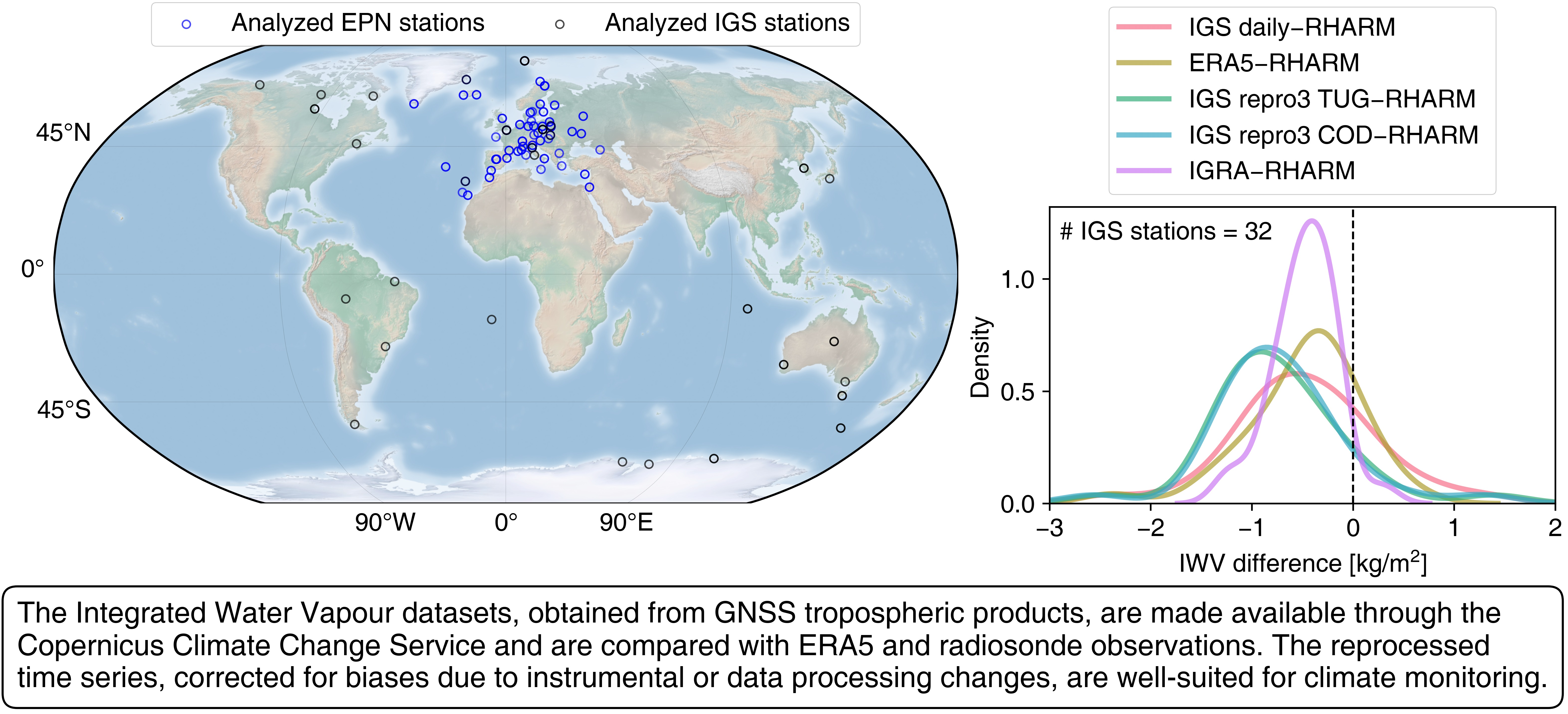
Based on GNSS tropospheric outputs from various geodetic networks (global or regional), we seek to provide standardized GNSS IWV datasets for climate research. A daily NRT IWV from the IGS network, whose initial data were collected via the Crustal Dynamics Data Information System (CDDIS) data portal [49], and the EPN-repro2 [44] are released in CDS as a first step. Both IGS and EPN as geodetic reference networks (Figure 1) are known for the state-of-the-art technical requirements on the GNSS sites and transparent quality assessment. The future development of this activity is to continue adding IWV datasets based on reprocessed GNSS data to support climate research. The IGS repro3 IWV dataset is under implementation in CDS. The same algorithm can be used in the future to add to the CDS any new GNSS IWV data based on publicly accessible reprocessed GNSS tropospheric products.
For the provision of Zenith Total Delay (ZTD), we are aware that the data processing and analysing institutions/agencies for any networks use their own best practices and try to follow the highest known standards for providing ZTD. It must be noted that the GNSS analysis centres use a variety of software tools, approaches and configurations (e.g., [50]), each of which has the potential to have a varied impact on the IWV values. However, since this is outside the purview of our investigation, this paper does not quantify the precise impact of algorithms and software on IWV values. Reprocessed items should be considered “already harmonized” and “useable as is”.
The IGS collects, archives and freely distributes GNSS observation datasets from a cooperatively operated global network of more than 500 ground tracking stations. The IGS network has been classified as a reference network according to the Measurement System Maturity Matrix (MSMM) [51], ensuring open access and high-quality GNSS data products since 1994. The IGS data processing agencies deliver the daily GNSS troposphere products available at CDDIS in a unified (SINEX TRO) format [52]. These ZTD time series are still not adjusted for any effects originating from instrumental changes (receivers, antennas, or radomes) or changes in station environment (like the growth of canopy or rising new buildings disturbing the open horizon for GNSS antennas) or earthquakes [53]. The GNSS time series adjustment requires specific reprocessing [54,55] (carried out within IGS and EPN reprocessing campaigns). The IGS NRT (daily) dataset is pertinent in atmospheric investigations while not ideally suited for climate studies due to its global coverage and rather short latency (approximately 2–3 weeks).
The EPN repro2 (Figure 1) is a reprocessed dataset that, similarly to the IGS dataset, is obtained from a reference quality GNSS network [56]. It consists of 18+ years of GNSS data belonging to the EPN and, therefore, is a valuable dataset for developing a climate data record of GNSS tropospheric products over Europe. For EPN repro2, five ACs homogeneously reprocessed its data for 1996–2014 [56]. ZTD screening is a process of inspecting data for identifying or detecting errors, and correcting them before performing data analysis, allowing the removal of all the estimated offsets (biases) induced by changes in GNSS hardware (e.g., antenna or radome) or adjacent environments [56]. It has been applied to all initial EPN repro2 ZTD time series [56]. The daily ZTDs provided by the EPN ACs are combined weekly. Only sites with a corresponding coordinate solution and three individual AC contributions are presented. Estimates with standard deviation (STDDEV) > 15 mm are excluded. Strong outliers are also detected and removed. Details on the combination process can be found in [57]. The data processed and transmitted by EPN (in EPN-repro2) should be regarded and understood as a distinct product if any of the sites belong to more than one network (for example, official IGS sites in EPN).
The current spatial density and global coverage of the available GNSS IWV datasets are insufficient and limit their capabilities in studying water vapour variability at different spatio-temporal scales. Regional and national geodetic networks have great potential for densifying the global GNSS network (IGS, together with EPN, offers a relatively dense network over Europe and adjacent areas, and provides unified homogeneous ZTD and IWV archives).
2.1.2. Implementation
According to recommendations in [58], a screening is initially applied to ZTD values and uncertainty. The data processing schema follows a similar methodology to that employed for the NGL-enhanced dataset [35] but it covers all IGS locations from 2000 to 2023. An evaluation of IWV uncertainty is incorporated into the data processing technique. This permits the assessment of statistical concordance among results produced from multiple independent methodologies in conjunction with the IWV time series.
Two main parameters for each dataset are provided to the CDS: GNSS ZTDs, provided as delivered to and available in CDDIS, and IWV. The latter is an entirely new product and made available, for the first time, exclusively for the CDS using an algorithm that mimics the GRUAN Data Product for GNSS data and observational uncertainties introduced in [59]. Both IGS and EPN repro2 ZTD and IWV are provided at hourly temporal resolution. Additionally, the database comprises GNSS site metadata, the weighted-mean temperature of the atmosphere, and IWV retrieved from hourly ERA5 data. The process involves bilinear interpolation from a 0.25 × 0.25 degree grid to match the geographical coordinates of the site and integrating humidity from the GNSS station’s altitude upwards.
The metadata used for estimating GNSS IWV and its uncertainty is described in Appendix A. The site metadata (e.g., site coordinates) can be found in IGS sites’ specifications and from the SINEX TRO files’ headers. It has proven challenging to use file headers because of inconsistent or missing data. From practical considerations, the software implementation of the IWV processing uses SEMISYS [60].
Additionally, the auxiliary meteorological data for converting ZTDs into IWV is needed for estimating as defined in [61,62]. There are two main possibilities for estimating . The first option is to use linear approximation from the near-surface air temperature, , as proposed by Bevis et al. [8] ( = 70.2 + 0.72). Another possibility would be to estimate using NWP models or reanalysis data (e.g., ERA5). On the one hand, using ERA5, the GNSS IWV estimates depend on reanalysis and cannot be used as an independent validation option for the models and reanalysis itself [13]. Alshawaf et al. [14] have shown that temperature and pressure data from reanalysis can lead to a bias in IWV compared to the use of surface measurements, especially in mountainous regions. Therefore, they recommended using Bevis’ approximation based on . For the same reason, the approximation has been chosen for atmospheric water vapour trends analysis in Switzerland [13], where the surface pressure, and at the GNSS station are vertically interpolated from pressure and temperature measurements at the closest meteorological station, assuming hydrostatic equilibrium and an adiabatic lapse rate of 6.5 K km.
On the other hand, the use of near-surface air temperature as an approximation for may prove inadequate during certain seasons and in specific geographic regions (e.g., Arctic [63]), where regional linear regression models that differ but are similar could be applied [64,65]. In addition, the approach assumes well-established data flow from ground-based meteorological stations. In [62], it was concluded that the most common practice for estimating , i.e., using the − relationship, is not suitable for global estimation because of the diurnal bias and the difficulties in obtaining site-, time- and even weather-dependent − relationships. The same issues with linear approximation are mentioned in [66,67,68] which advocate for the utilization of NWP data instead.
The measurements from radiosoundings and meteorological stations are assimilated into ERA5. However, it is important to note that many other observations (e.g., satellite-based radiance measurements) and factors (e.g., the characteristics of forecast models and the procedures used for data assimilation) influence reanalysis like ERA5. Therefore, comparing radiosonde and reanalysis is still a worthwhile endeavour. As found by [35] the difference between the from ERA5 and radiosondes is negligible. There have been few independent analyses of ERA5’s estimations of tropospheric temperature. Only one study by Graham et al. [69] that matched independent campaign-based radiosonde temperature profiles with ERA5 data was found. This investigation demonstrated that ERA5 provides a good estimate of Arctic tropospheric temperature.
For the CDS GNSS dataset, the impact of estimation on GNSS IWV values from based approximation is discussed in Section 3.1. In light of the arguments for NWP and reanalysis, as well as from a practical standpoint, we have chosen retrieval from reanalysis as recommended for climate applications. The ERA5 parameters needed for calculating used in ZTD to IWV conversions are geopotential height, specific humidity and temperature at 37 pressure levels https://cds.climate.copernicus.eu/cdsapp#!/dataset/reanalysis-era5-pressure-levels?tab=overview (accessed on 24 October 2023).
The technical implementation and access to the data portal are described in Appendix A and Appendix B, respectively.
2.2. Study Setup and Analysis Method
A thorough assessment of the IWV values present in the CDS GNSS datasets was made against co-located and harmonized data from the Radiosounding HARMonization (RHARM; [70]) approach spanning the period from 2000 to 2021 (Section 3.2). The RHARM method has been applied to modify twice-daily radiosonde data collected at 16 pressure levels in the range of 1000 to 10 hPa. These specific levels are consistently available at the stations for each ascent. Relative humidity (RH) data are limited to 250 hPa due to widespread sensor performance issues at higher altitudes in most commercial sondes [71]. The applied adjustments are interpolated to all reported levels (including significant level reports that differ in the definition for each profile). On average, we had access to and utilized data from 30 levels in the analysis for each radiosounding. The data covers 697 stations from 1978 to the present and is sourced from the Integrated Global Radiosonde Archive (IGRA). Importantly, the RHARM-adjusted data stand as an entirely self-contained dataset, free from any dependencies on reanalysis data. The evaluation aimed to assess the performance of the GNSS datasets in precisely estimating IWV on a worldwide scale. The analysis was conducted using data only from stations and dates for which estimates from all six datasets—RHARM, IGRA, IGS NRT, IGS repro3 TUG (from Graz University of Technology), IGS repro COD (from Center for Orbit Determination in Europe) and ERA5—were available. In addition, only data from co-located GNSS and radiosonde stations meeting the following criteria were considered:
- Having the same report timestamp;
- A distance difference of less than 30 km;
- An elevation difference within 100 m;
- Containing at least 6 months of data.
To classify the co-located measurements into “day” and “night” values, an approach based on the solar elevation angle (SEA) was employed. The SEA is determined by time, latitude and longitude, and was calculated using the suncalc library implemented in the Python language [72]. IWV values were considered “day” measurements if the SEA ranged from 0 to 90 degrees, while “night” measurements were defined when the SEA ranged from −90 to 0 degrees. In total, 58,095 daytime measurements from 32 stations and 42,048 nighttime measurements from 29 stations were used (Figure 1; the full list of IGS stations used can be found in Appendix C). For IWV trend analysis, only stations with more than 10 years of data were included.
A separate analysis was explicitly performed for EPN stations covering the period from 1996 to 2014 (Section 3.3). However, in this comparison, the radiosonde data were excluded since, in Europe, there is limited availability of co-located radiosonde and GNSS stations that offer extensive and long-term datasets suitable for IWV climatology studies. This allowed us to broaden the scope of the analysis to include a larger number of stations and data at all full hours spanning from 00 to 23 UTC to study the IWV differences and trends for GNSS-based datasets and ERA5. The analysis is confined to the European region, including 2,276,093 nighttime and 2,315,494 daytime IWV values from 61 EPN stations. Out of these stations, 42 stations with more than 10 years of data were selected for studying IWV trend differences (Figure 1, the full list of EPN stations employed can be found in Appendix C).
Finally, an intercomparison study between IGS NRT, IGS repro3 datasets from ACs TUG and COD, and co-located GRUAN-processed Vaisala RS92 radiosonde (RS92-GDP.2) was conducted for two IGS stations, NYA1 and TSKB, both of which boast extensive data records. Notably, these stations are in close proximity to GRUAN stations Ny-Alesund and Tateno, at distances of only 1.7 and 6.4 km, respectively. These GRUAN stations are among the longest-operated in the network. As a result, the study encompassed data from 2006 to 2018 for NYA1 and from 2009 to 2020 for TSKB. (Section 3.4). GRUAN measurements offer valuable, extended-term and high-precision climate data records, spanning from the Earth’s surface through the troposphere and into the stratosphere. Importantly, quantifiable uncertainties are always provided for these measurements. The RS92-GDP.2 data are available for registered users at the GRUAN file archive https://www.gruan.org/data/file-archive/rs92-gdp2-at-lc/ (accessed on 24 October 2023).
The two radiosonde datasets used in the current study exhibit a fundamental distinction: RHARM solely offers data at significant and mandatory levels, whereas GRUAN provides data with much higher resolution (typically 5–10 m). To enable comparison with GNSS data, the water vapour data from radiosonde profiles were integrated upward from the altitude of the GNSS station. The humidity value at the lowest level was determined using linear interpolation or extrapolation. It has been found that this step introduces an additional uncertainty of around 0.5% in relative humidity measurements in the case of RHARM [70]. Regarding the uncertainty for GRUAN IWV, its values were directly taken from the RS92-GDP.2 data files without any modifications or adjustments. For the uncertainty of RHARM IWV values, the estimation is made according to the latest scheme developed by GRUAN [73], which, in turn, follows the guidelines in the Guide to the Expression of Uncertainty in Measurement (GUM) [74]. Due to the non-instantaneous nature of radiosonde measurements (usually lasting more than an hour) and their potential drift during ascent, an additional collocation mismatch uncertainty must be taken into account [75], impacting the consistency between GNSS and radiosonde data. Also, GNSS IWV represents the measurement of an inverted atmospheric cone, covering a diameter of approximately 45–75 km at an altitude of 2 km when GNSS data is collected at an elevation of 3–5 degrees. However, using the relatively strict collocation criteria described above, and considering that the temporal and spatial variation of IWV in the vicinity of measurement sites is small, this effect was neglected. A straightforward screening step was established as part of the data processing and quality control process to eliminate RHARM profiles if they contained data at fewer than ten pressure levels (usually, depending on the station, only a small percentage of profiles were excluded).
Linear trends in the IWV were estimated for all datasets using the model [76]:
where y and t are the IWV and the time in years, respectively. All unknown coefficients are estimated using the method of least squares. The parameters and describe the mean and the linear trend of the IWV. The parameters and represent the amplitude and phase of the annual variation in the IWV time series. Similarly, the parameters and are the semi-annual component coefficients. To account for the variability and relationships within the data, the covariance matrix is needed to estimate the trend uncertainties [42]. The best-fit parameters and the respective covariance matrix (two-dimensional array) were calculated using an open-source software SciPy [77,78] algorithm (version 1.7.3). The diagonal elements of the array give the square of the uncertainties of the best-fit parameters.
The consistency test used for assessing the agreement between the two datasets is based on the approach proposed by Immler et al. [79]. This method takes into account two independent measurements, and , and their respective standard uncertainties, and , for checking a pair of independent measurements for consistency:
where for GNSS IWV is calculated according to Ning et al. [59] and for the radiosonde according to [73]. In this work, the level of consistency between two measurements is determined as strong, moderate or weak if Equation (2) holds for , or , respectively. Additionally, the Pearson correlation coefficient is used to measure linear correlation between two datasets.
3. Results
3.1. The Impact of Estimation Approaches on IWV Value
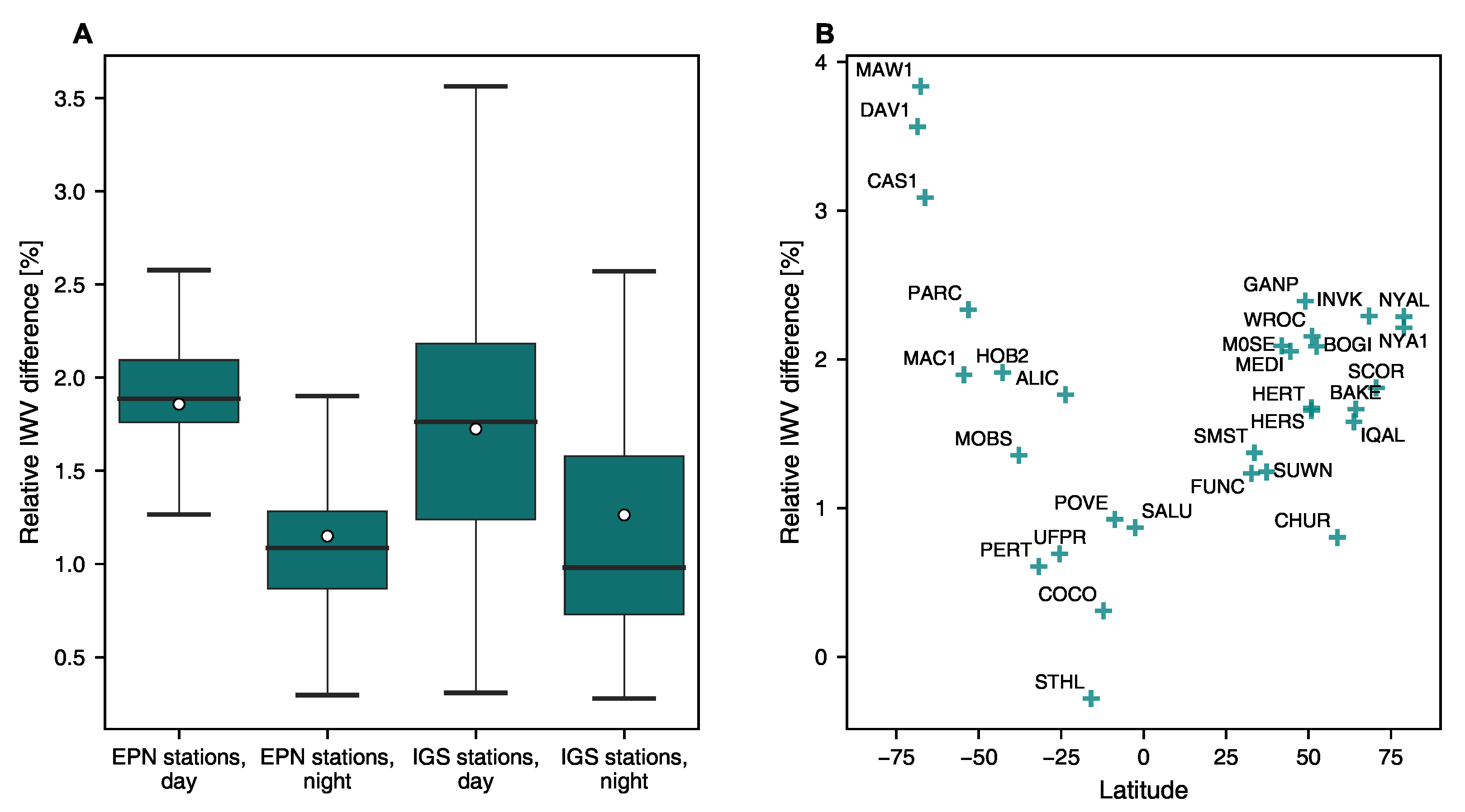
The IWV estimates based on derived from ERA5 temperature and humidity profiles, and estimated by using the from ERA5 are compared to evaluate these approaches’ agreement and potential impact on IWV values. The simplification for calculating presented in Bevis et al. [8] increases the IWV at EPN and IGS stations during daytime by more than 1.8% on average (Figure 2). The respective increase at night is approximately 1%. These results indicate that the derived from has a more noticeable diurnal dependency than the calculated from temperature and humidity profiles. Additionally, it is found that the simplification used for has a latitude-dependent impact on IWV. The effect is most pronounced at high latitudes, with a significant increase of up to 4% at some Antarctic stations. The discovery regarding the latitudinal dependency of agrees with the previous research conducted by Wang et al. [62]. Based on the calculated from GRUAN radiosonde temperature and humidity profiles in Section 3.4, the derived from the lowest level of radiosonde profile, taken as , is overestimated at Ny-Alesund (3774 soundings) and Tsukuba (1951 soundings) by 10.0 K and 4.8 K, respectively. On the other hand, the mean ERA5 minus GRUAN difference, calculated from profiles, is only 1.2 K and −0.6 K, respectively. These findings emphasize the value of utilizing ERA5-derived in climate studies, as already discussed in the literature, e.g., [80].
3.2. Intercomparison of IWV and Its Trends at IGS Stations
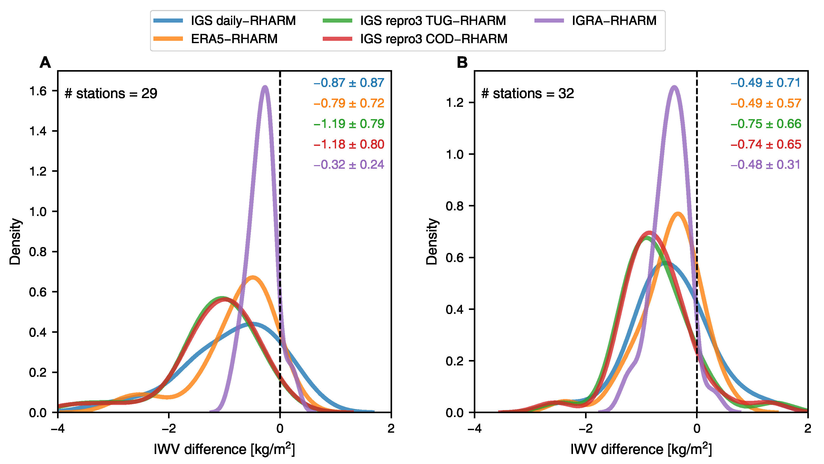
The analysis made for approximately 30 IGS stations indicates a consistent but minor “dry” bias of IWV across all the evaluated datasets derived from the GNSS technique (Figure 3). The IWV values obtained from the RHARM dataset consistently exceed the unadjusted IGRA IWV on average by 0.3 ± 0.2 kg/m (mean ± standard deviation) during nighttime and 0.5 ± 0.3 kg/m during daytime. The GNSS-based reprocessed IWV time series show a negative difference from RHARM, ranging from −0.7 kg/m (−6%) during the day to −1.2 kg/m (−10%) at night. It is worth noting that the un-reprocessed IGS daily dataset exhibits a relatively smaller discrepancy, around 0.3 kg/m (4%) higher in moisture compared to the reprocessed GNSS IWV, aligning closely with those derived from ERA5.
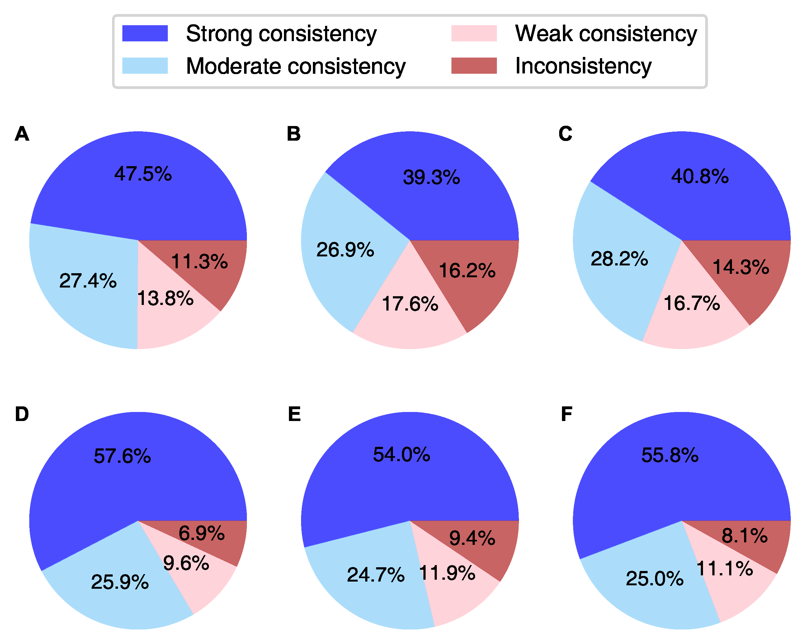
Considering their known uncertainties, Equation (2) was applied pair-wise to study the agreement between the GNSS-derived IWV and the value calculated from RHARM humidity profiles (Figure 4). The average IWV uncertainties at nighttime in the IGS daily product, IGS repro3 provided by TUG and IGS repro3 provided by COD are 0.5, 0.3 and 0.4 kg/m, respectively. Consequently, approximately 48%, 39% and 41% of the IWV values exhibit strong consistency with RHARM estimates, considering that the average uncertainty of RHARM IWV is 1.3 kg/m. If the uncertainties have a normal distribution, these percentages are fairly close to the amount of agreement that was expected. At the same time, the fraction of inconsistent measurements slightly exceeds 10%, implying that one of the uncertainties may be larger than initially estimated. Conversely, during the daytime, approximately 58%, 54% and 56% of the IWV estimates exhibit strong agreement for the IGS daily product, IGS repro3 from TUG and IGS repro3 from COD, respectively. The enhanced daytime agreement is the result of two factors: reduced average discrepancies in IWV and higher uncertainty estimates for RHARM, which are 1.5 kg/m on average. The uncertainty of RHARM IWV clearly depends on the actual IWV content itself and, consequently, on the station’s latitude. Its value ranges from 0.5 kg/m at the high-latitude radiosonde stations Ny-Alesund II (78.92N, 1.4 km from the IGS station NYAL) and Mawson (67.60S, 0.4 km from MAW1) to more than 2.5 kg/m at the equatorial stations Cocos Island (12.19S, 0.1 km from COCO), Porto Velho (8.77S, 6.7 km from POVE) and Sao Luiz (2.6S, 2.4 km from SALU). The finding is consistent with IWV uncertainties given for GRUAN radiosoundings [73]. However, RHARM IWV’s uncertainty is higher than the value reported for GRUAN measurements. This can be attributed to the fact that RHARM uncertainties for relative humidity and temperature are higher (see also [70]), and the profiles have a lower vertical resolution. A negligible daytime/nighttime difference in uncertainty is observed for the GNSS-based IWV measurements. The marginal enhancement in agreement between RHARM and TUG-provided IGS repro3, compared to the agreement between RHARM and COD-provided IGS repro3, can be solely attributed to the slightly higher uncertainty associated with the IWV estimates from TUG.
The trends in nighttime and daytime RHARM IWV at the co-located IGS stations shown in Figure 1 are −0.35 and 0.15 kg/m per decade, respectively. The average trend uncertainties derived from the covariance matrix (see Section 2.2) are 0.23 and 0.24 kg/m, respectively. The uncertainties in IWV trends during nighttime are smaller than the actual magnitude of the trends at all six radiosonde stations under consideration, which are in proximity to IGS stations CHUR, HERS, HOB2, MAC1, SUWN and WROC. This is also true for eight out of ten stations during daytime (WROC and HOB2 being the only exceptions). This indicates that the length of the time series used is appropriate for detecting long-term changes at most of the selected stations. It is crucial to stress that there is significant variability in the IWV trend values across various sites. The standard deviation of the RHARM IWV trend calculated over all sites is approximately 0.7 kg/m per decade. The stations selected for the analysis of IWV trends are situated across the globe, spanning from 79N to 66S latitude, although not encompassing all continents. Consequently, the estimated trend values may not accurately represent the global IWV climatology across various regions. However, comparing the methods can still shed light on the accuracy of GNSS datasets for studying IWV trends. The datasets derived from IGS repro3 show slight discrepancies compared to the results obtained from RHARM regarding the IWV trends for both nighttime and daytime periods. Based on both reprocessed GNSS IWV datasets the average daytime and nighttime IWV trends are −0.23 and 0.02 kg/m per decade, respectively. Similarly to the results from RHARM data, the nighttime and daytime IGS repro3 IWV trends are statistically significant. This holds true for five out of six stations (with the exception of HERS) for nighttime and nine out of ten stations (excluding ALIC) for daytime trends. Moreover, the uncertainty ranges of IWV trends from RHARM and IGS repro3 datasets overlap at most stations, further highlighting the similarity in the trend estimation. It is important to note that the most significant discrepancies from the RHARM IWV trends are observed for the IGS daily solution at night and the IGRA dataset during the daytime. In the case of the former, the average IWV trend difference from RHARM reaches −0.3 kg/m per decade. In the latter case, the difference is around +0.2 kg/m per decade. Therefore, these unadjusted datasets are not suitable for detecting long-term changes in IWV values.
3.3. Intercomparison of IWV and Its Trends at EPN Stations
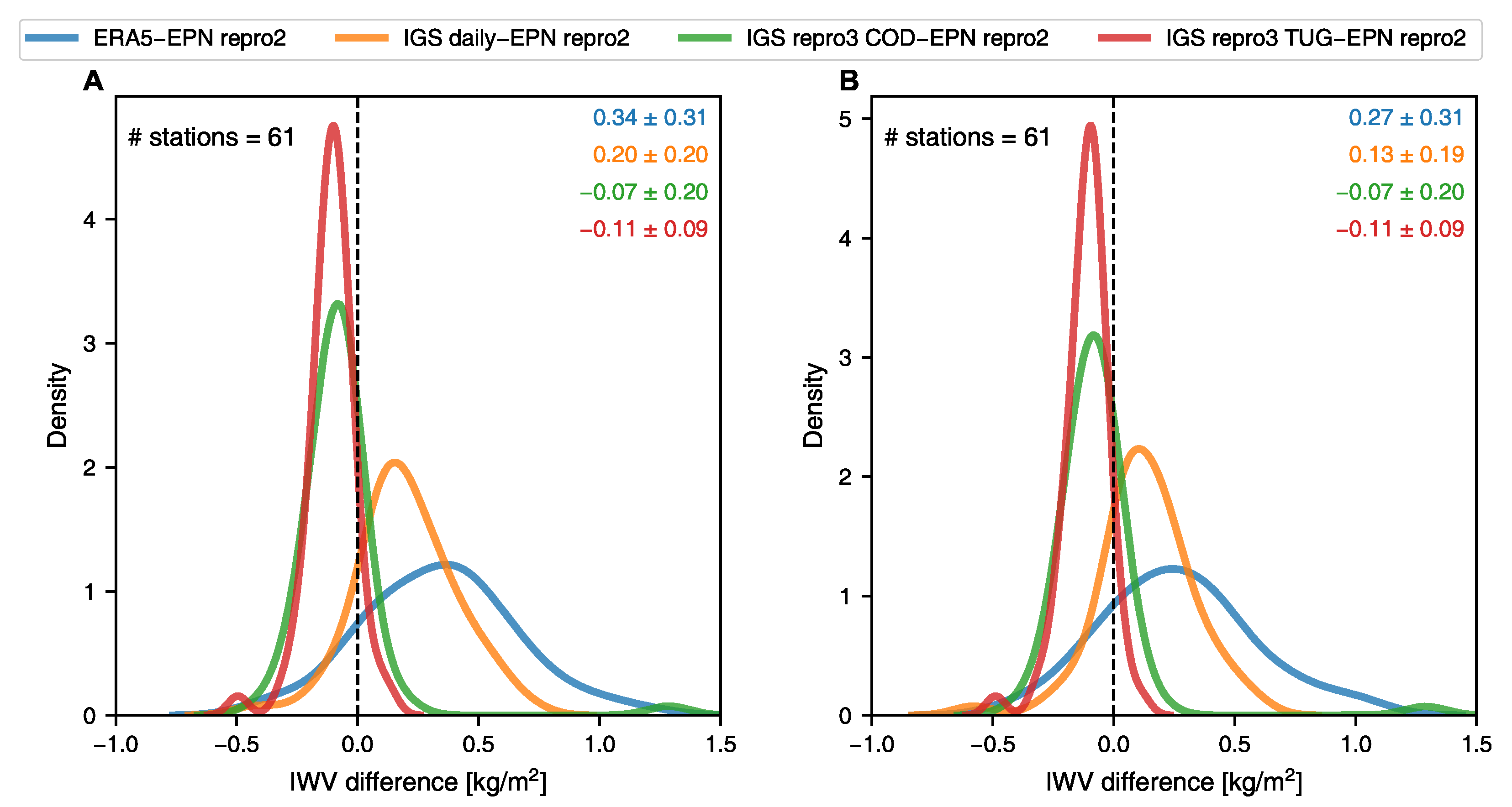
Figure 5 illustrates the differences in IWV among the ERA5, IGS daily product and IGS repro3 datasets, and the EPN repro2 dataset (the sites used in this comparison can be found from Appendix C). The analysis reveals that the EPN repro2 dataset lies between the relatively “wet” solutions provided by ERA5 and the IGS daily product, and the comparatively “dry” solutions offered by the two IGS repro3 datasets. The behaviour observed in the EPN repro2 dataset is similar to the results of the IGS stations investigated in the previous section. The average difference in IWV between the IGS repro3 datasets and EPN repro2 does not exceed 0.11 kg/m. This suggests that, in general, reprocessing strategies yield similar solutions when it comes to IWV estimates. The difference between ERA5 and IGS daily IWV from EPN repro2 is larger, ranging from 0.19 to 0.34 kg/m.
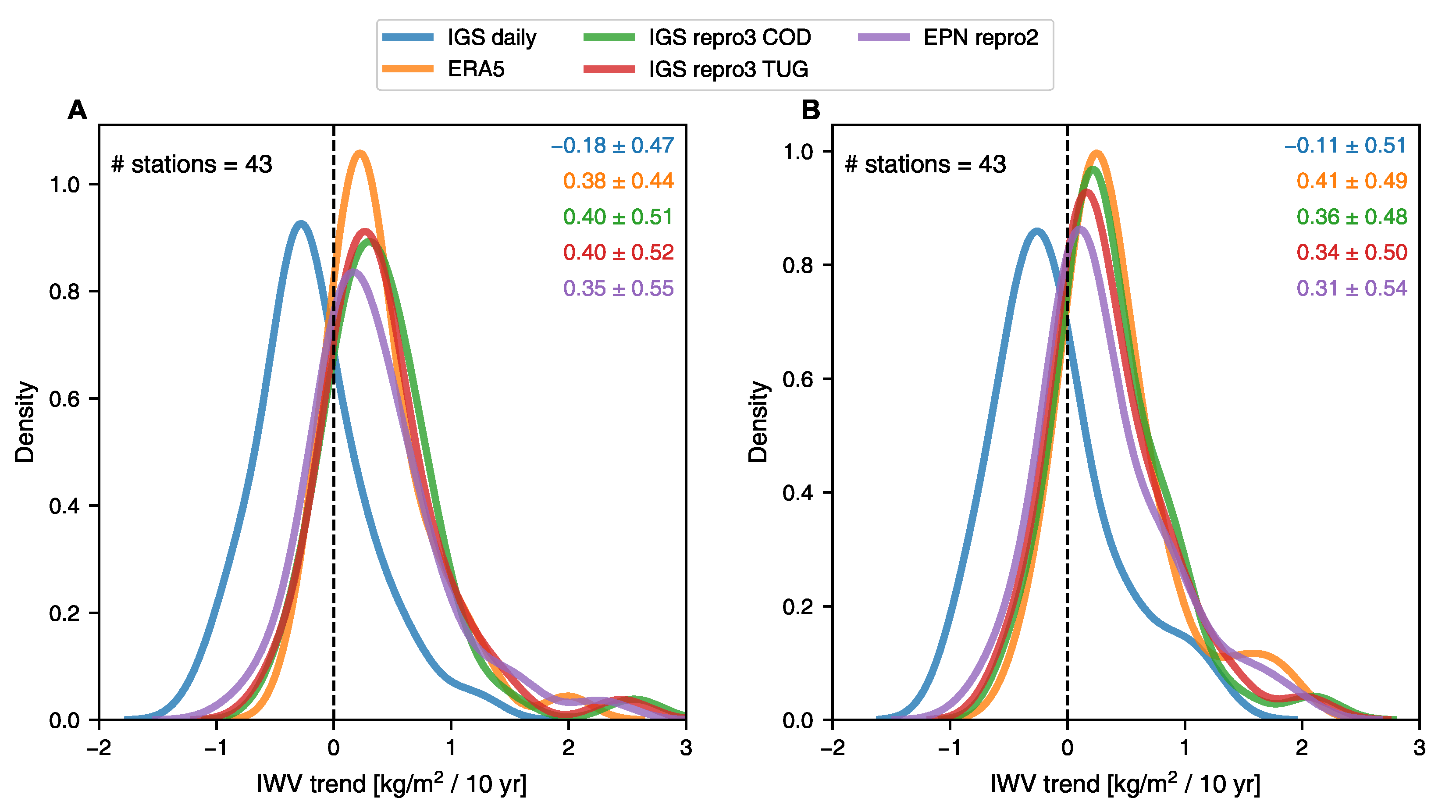
In the analysis of IWV trends at EPN stations, it is observed that there is a strong agreement between ERA5, IGS repro3 and EPN repro2 datasets (Figure 6). The IGS repro3 datasets provided by the two ACs show negligible differences, less than 0.03 kg/m per decade. The average IWV trend values range from +0.3 to +0.4 kg/m per decade during nighttime and daytime, respectively, with an average uncertainty of 0.02 kg/m per decade. The standard deviation of the trend calculated over all stations is around 0.5 kg/m. Also, the trends in ZTD time series can be seen (on average, from 0.5 to 1.4 mm per decade based on nighttime and daytime EPN repro2 data, respectively). A significant discrepancy is observed when comparing the results from the IGS daily solution with other datasets analysed. The IGS daily solution shows more negative IWV trends by −0.5 kg/m compared to EPN repro2, IGS repro3 and ERA5. This tendency is consistent with the findings in Section 3.2 for the fewer stations at the global level. This indicates that the IGS daily solution does not capture the overall positive IWV trend detected in Europe using other datasets.
3.4. Intercomparison of IWV at Two GRUAN Stations
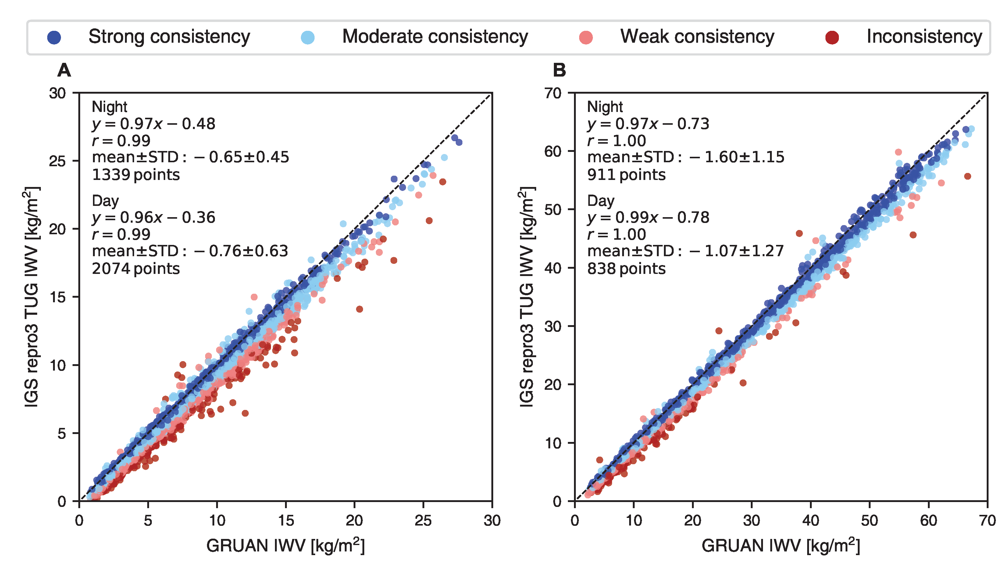
The IWV estimates derived from the reprocessed GNSS data recorded at NYA1 and TSKB by TUG exhibit deviations of −0.7 and −1.5 kg/m (equating to reductions of −14% and −6%) during nighttime measurements, respectively, compared to the corresponding values obtained from the GRUAN radiosonde dataset (Figure 7). Similarly, a negative IGS repro3 from TUG minus GRUAN IWV difference during daytime is found for these stations at night: −0.7 and −0.9 kg/m (9% and 4%), respectively. The datasets offered by the two IGS ACs show very small differences, less than 0.07 kg/m at both stations on average. The GNSS-based and GRUAN-estimated IWV consistency percentages are comparable for all three IGS datasets. When comparing the IGS daily product, the “strong consistency” portion is where the major difference is most evident, exhibiting approximately 10% higher agreement compared to the reprocessed datasets (results given only for IGS repro3 by TUG in Table 1). Approximately 32% of the simultaneous co-located measurements are strongly consistent and 6% are inconsistent. The results indicate a slightly reduced “strong consistency” fraction and show an increase in the “inconsistency” fraction compared to the GNSS and RHARM IWV comparison (Section 3.2).
The results support earlier reports [81] that there is a small dry bias in GNSS-based IWV measurements. Assuming a random collocation mismatch error, the ideal situation would be for 50% of the values in each consistency category to show one method displaying greater IWV values than the other. Only 3% and 8% of the daytime data at NYA1 and TSKB, respectively, reveal higher IWV compared to the GRUAN. Additionally, there were no instances of greater IWV during the night in the GNSS datasets compared to the GRUAN. At the same time, if using the value of the intercept, a very high correlation is observed between the IWV values derived from the GNSS-based datasets and the GRUAN radiosonde. The Pearson correlation coefficient exceeds 0.98 for both day and night measurements at both stations.
4. Discussion
In this study, ERA5, several GNSS and radiosonde datasets were compared in order to assess how well a novel algorithm worked in producing the first standardized global GNSS IWV dataset with uncertainties made accessible by the Copernicus Climate Change Service. All the data used in the study are currently available or will soon be accessible at the C3S CDS. The GNSS-based IWV calculations are accurate for analysing IWV trends, according to the examination of the global reprocessed GNSS and radiosonde datasets. As expected, compared to the reprocessed GNSS datasets, the un-reprocessed dataset shows larger differences from IWV trend estimates calculated using RHARM post-processed data. This finding supports the use of homogenized GNSS datasets, such as the IGS repro3 or EPN repro2, for climate investigations. Contrarily, it has been found that the average IWV difference between the homogenized GNSS and radiosonde time series tends to be slightly bigger than the difference between the corresponding unhomogenized data. Because the homogenization method may have an impact on the dataset’s quality and produce a persistent bias, the finding requires more investigation. The negative GNSS minus radiosonde bias found in the current study has also been presented in several earlier studies, such as [82], even using homogeneously reprocessed GNSS data [83]. According to the investigation of uncertainties, the global reprocessed GNSS and radiosonde (RHARM or GRUAN) datasets clearly show substantial agreement, especially during the daytime. A high level of agreement among the different reprocessing campaigns in capturing the IWV values and trends was found using data collected for EPN and global IGS stations. Future research can extend the current study’s reach in the context of IWV trends by including noise models in trend analysis, using, for example, a methodology discussed in previous studies by Alshawaf et al. [14] and Klos et al. [84].
The outcomes of the intercomparisons conducted with GNSS, radiosonde and reanalysis IWV time series are influenced by several factors, including the chosen study period, geographical scope and the specific set of monitoring sites. Furthermore, systematic differences and trends seen in IWV are strongly influenced by how much harmonization is performed or by whether it is completely lacking. To the best of our knowledge, this study represents the first attempt to use a standardized method to estimate IWV uncertainties to compare reprocessed GNSS-derived IWV versus values obtained from post-processed radiosoundings and the most recent reanalysis. The results of this study cannot thus be directly compared to those of earlier research available in the literature. However, the size of the differences seen in the reconstructed GNSS IWV is close to what has been reported when using unhomogenized radiosonde data (e.g., [35]) or earlier-generation reanalysis datasets [56].
We regrettably lack unified open-access reprocessed datasets of tropospheric products acquired by densifying global coverage outside of Europe despite having thousands of reference-grade GNSS sites throughout the world. Finding and incorporating existing reprocessed GNSS tropospheric datasets into CDS, as well as encouraging international geodetic and climate research communities to work together for a geographically more dense and homogeneous representation of the IWV data for global climate research, are some of the long-term goals of C3S. The reprocessed GNSS IWV datasets in CDS are a first attempt to share open-access global GNSS-based data with a wide community.
Author Contributions
Conceptualization, K.R., H.K. and F.M.; methodology, K.R. and H.K.; software, K.R. and H.K.; validation, H.K. and F.M.; data analysis, H.K.; data curation, H.K.; writing—original draft preparation, K.R., H.K. and F.M.; writing—review and editing, K.R., H.K. and F.M.; visualization, H.K. All authors have read and agreed to the published version of the manuscript.
Funding
This work was carried out on behalf of the European Union’s Copernicus Climate Change Service implemented by ECMWF. Use of the CDS GNSS IWV and RHARM data as stated in the Copernicus license agreement is acknowledged. H.K. acknowledges support from the Estonian Research Council team grant PRG1726.
Data Availability Statement
The data is freely accessible in CDS data portal https://cds.climate.copernicus.eu/ (accessed on 24 October 2023) under “In-situ observations of water vapour and atmospheric delay from the ground-based GNSS network from 1996 to present”. All users of data uploaded on the Climate Data Store (CDS) must: provide clear and visible attribution to the Copernicus programme by referencing the web catalogue entry, acknowledge according to the data licence and cite each product used.
Acknowledgments
We acknowledge GFZ SEMISYS https://semisys.gfz-potsdam.de/semisys/ (accessed on 24 October 2023) for GNSS site metadata and Copernicus CDS service for meteorological data from ERA5 and RHARM datasets for comparative studies. This work was carried out on behalf of the European Union’s Copernicus Climate Change Service implemented by ECMWF. Use of the CDS GNSS dataset with the related uncertainties as stated in the Copernicus license agreement is acknowledged.
Conflicts of Interest
The authors declare no conflict of interest.
Appendix A. Technical Implementation of the Service
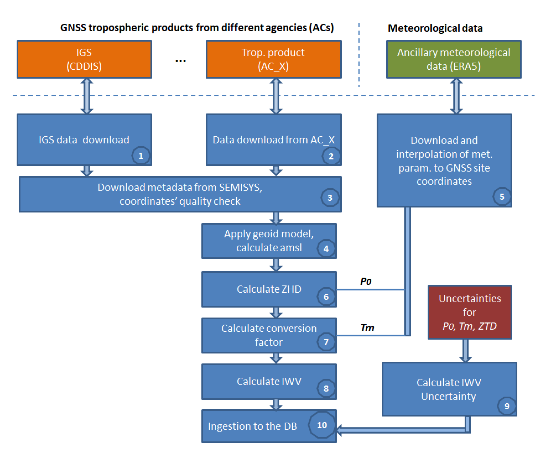
The technical implementation of the service is realized as an SQL database in CDS https://cds.climate.copernicus.eu/cdsapp#!/dataset/insitu-observations-gnss (accessed on 24 October 2023). The data follows the standard of Common Data Model (CDM) for in situ observations in cooperation with other C3S 311a lots, known as C3S CDM-OBS (available in the ECMWF internal repositories and the latest version at https://github.com/glamod/common_data_model/blob/master/cdm_latest.pdf (accessed on 24 October 2023)). The data processing schema and retrieval of GNSS IWV for both IGS and EPN tropospheric products are described in the ATDB document [85]. A simplified description of the data flow and the main data processing steps is depicted in (Figure A1):
- Pre-processing of GNSS troposphere product (1–4);
- Pre-processing of ancillary data (5–7);
- Calculating IWV and its uncertainty, ingestion to the DB (8–10).
Figure A1.
Retrieval of IWV for IGS and EPN repro2.

The pre-processing steps (1–4) are state-of-the-art techniques and the height above the mean sea level is calculated using the Earth Gravitational Model EGM2008, released by the National Geospatial-Intelligence Agency (NGA). The steps (5–8) with related formulas for calculating the Zenith Hydrostatic Delay (ZHD) and IWV values are described in [85].
The ZHD can be modelled as [86]:
where is the total pressure (in hPa) at the Earth’s surface, is the GNSS site latitude in degrees and H is the surface height above the geoid (height above the mean sea level) in meters. Calculating the Zenith Wet Delay (ZWD) from Zenith Total Delay (ZTD) follows:
The IWV estimates from ZWD are calculated by equations detailed in [8]:
where is the density of liquid water, is the specific gas constant for water vapour, is the water-vapour-weighted mean temperature of the atmosphere, and are the molar masses of water vapour and dry air, respectively, and , and are physical constants from the formula for refractivity [87,88].
The ancillary meteorological data from ERA5 is obtained by using CDS API (https://github.com/ecmwf/cdsapi, accessed on 24 October 2023) integrated to the backend software. The resulting values of GNSS IWV, the associated uncertainties and the site metadata, together with the complementary IWV values retrieved from ERA5, are ingested into the PostgreSQL database (step 10).
The novel GRUAN-like IWV uncertainty calculation (step 9) is based on [59] and accounts for uncertainties from all sources in the data processing chain:
where is the functional relationship between the GNSS IWV and input variables, and is the one-sigma uncertainty of the corresponding variable. This approach yields:
where , , , , , , and are the one-sigma uncertainties of IWV, ZTD, , the constant in the derivation in ZHD (see Equation (12) in [85]), the coefficient (), and the constants from a widely used formula for refractivity ( and ).
The IWV uncertainty calculation relies on previously published values for input variables used as constants with their uncertainties [8]: K/hPa, K/hPa, kg/m, , hPa (for ERA5), (dimensionless), K, K/hPa and K/hPa. The numerical values of (the formal errors interpreted as 1 uncertainties) are the final results of GNSS data processing delivered by ACs and are used “as is”. The uncertainties for and were determined statistically using IGRA and GRUAN radiosonde measurements, and align well with the results presented in several papers that specifically focus on ERA5 [89,90].
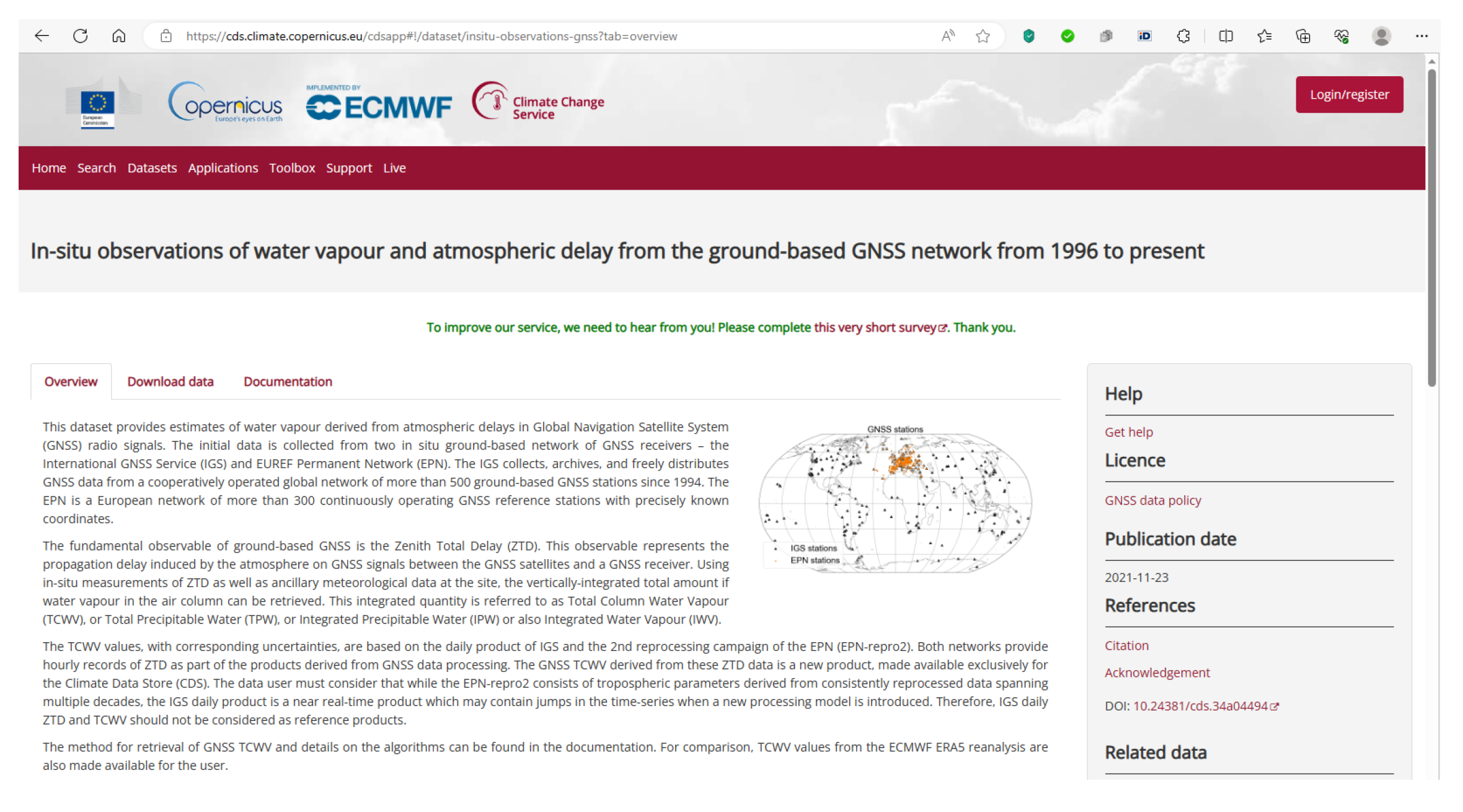
Appendix B. GNSS IWV in CDS Data Portal
The user can access the data in the CDS data portal https://cds.climate.copernicus.eu/ (accessed on 24 October 2023). By searching “GNSS”, the link to the “In-situ observations of water vapour and atmospheric delay from the ground-based GNSS network from 1996 to present” can be found and opened. The user gets redirected to the main GNSS in situ IWV observations’ web page (Figure A2) with three main sections.
The “Overview” section briefly overviews the available datasets, data description, and the main and related variables, as well as the GNSS data policy and citation rules. In the “Download data” section, the user can select the available networks, downloadable variables, the year, month and day of the observations, and the geographic area covered by the observations. The downloadable data can be chosen as a zipped file either by “CSV one row per report (zipped)” or “CSV one row per observation (zipped)”. The downloadable is a CSV file following the CDS convention CDM-OBS. In the “Documentation” section, the user can find the Product User Guide and Algorithm Theoretical Basis Description.
Figure A2.
In situ observations of water vapour and atmospheric delay from the ground-based GNSS network from 1996 to present in CDS.
Figure A2.
In situ observations of water vapour and atmospheric delay from the ground-based GNSS network from 1996 to present in CDS.

Appendix C. Stations Used in the Study

Table A1.
IGS stations employed for IWV comparison between IGS repro3 TUG, IGS repro3 COD, IGS daily, ERA5, IGRA and RHARM. Trend analysis was conducted using the sites indicated with a plus sign. The distance indicates the extent of separation between GNSS and radiosonde stations.
Table A1.
IGS stations employed for IWV comparison between IGS repro3 TUG, IGS repro3 COD, IGS daily, ERA5, IGRA and RHARM. Trend analysis was conducted using the sites indicated with a plus sign. The distance indicates the extent of separation between GNSS and radiosonde stations.
| GNSS ID | Lat, ° | Lon, ° | Trend | Radiosonde ID | Distance, km | No. Night Meas. | No. Day Meas. |
|---|---|---|---|---|---|---|---|
| ALIC | − 23.67 | 133.89 | + | ASM00094326 | 13.89 | 23 | 1778 |
| BAKE | 64.32 | −96 | − | CAM00071926 | 0.17 | 1680 | 2030 |
| BOGI | 52.47 | 21.04 | − | PLM00012374 | 9.19 | 1478 | 1822 |
| CAS1 | −66.28 | 110.52 | + | AYM00089611 | 0.18 | 758 | 2705 |
| CHUR | 58.76 | −94.09 | + | CAM00071913 | 3.14 | 2545 | 2820 |
| COCO | −12.19 | 96.83 | + | CKM00096996 | 0.11 | 698 | 3572 |
| DAV1 | −68.58 | 77.97 | − | AYM00089571 | 0.39 | 610 | 1878 |
| FUNC | 32.65 | −16.91 | − | POM00008522 | 1.78 | 0 | 764 |
| GANP | 49.03 | 20.32 | − | LOM00011952 | 0.48 | 1434 | 1489 |
| HERS | 50.87 | 0.34 | + | UKM00003882 | 3.82 | 1949 | 1574 |
| HERT | 50.87 | 0.33 | − | UKM00003882 | 3.76 | 1723 | 1258 |
| HOB2 | −42.8 | 147.44 | + | ASM00094975 | 6.19 | 3117 | 3595 |
| INVK | 68.31 | −133.53 | − | CAM00071957 | 1.24 | 2109 | 2546 |
| IQAL | 63.76 | −68.51 | − | CAM00071909 | 2.05 | 1268 | 1214 |
| M0SE | 41.89 | 12.49 | − | ITM00016245 | 25.07 | 347 | 370 |
| MAC1 | −54.5 | 158.94 | + | ASM00094998 | 0.08 | 2803 | 3131 |
| MAW1 | −67.6 | 62.87 | − | AYM00089564 | 0.4 | 252 | 1314 |
| MEDI | 44.52 | 11.65 | − | ITM00016144 | 15.02 | 2021 | 1047 |
| MOBS | −37.83 | 144.98 | − | ASM00094866 | 22.15 | 2806 | 2770 |
| NYA1 | 78.93 | 11.87 | + | SVM00001004 | 1.4 | 900 | 1845 |
| NYAL | 78.93 | 11.87 | − | SVM00001004 | 1.41 | 660 | 967 |
| PARC | −53.14 | −70.88 | − | CIM00085934 | 15.05 | 189 | 950 |
| PERT | −31.8 | 115.89 | + | ASM00094610 | 16.41 | 2052 | 2762 |
| POVE | −8.71 | −63.9 | − | BRM00082824 | 6.76 | 1313 | 1818 |
| SALU | −2.59 | −44.21 | − | BRM00082281 | 2.43 | 1046 | 1586 |
| SCOR | 70.49 | −21.95 | − | GLM00004339 | 0.11 | 1568 | 1729 |
| SMST | 33.58 | 135.94 | − | JAM00047778 | 21.89 | 74 | 46 |
| STHL | −15.94 | −5.67 | − | SHM00061901 | 0.07 | 0 | 1290 |
| SUWN | 37.28 | 127.05 | + | KSM00047122 | 21.46 | 2672 | 2683 |
| TSK2 | 36.11 | 140.09 | − | JAM00047646 | 6.32 | 81 | 50 |
| TSKB | 36.11 | 140.09 | − | JAM00047646 | 6.31 | 102 | 56 |
| UFPR | −25.45 | −49.23 | − | BRM00083840 | 9.97 | 1435 | 1670 |
| UNBJ | 45.95 | −66.64 | − | CAM00071701 | 20.72 | 13 | 36 |
| WROC | 51.11 | 17.06 | + | PLM00012425 | 12.63 | 2547 | 3036 |
Table A2.
EPN stations employed for IWV comparison between IGS repro3 TUG, IGS repro3 COD, IGS daily, ERA5 and EPN repro2. Trend analysis was conducted using the sites indicated with a plus sign.
Table A2.
EPN stations employed for IWV comparison between IGS repro3 TUG, IGS repro3 COD, IGS daily, ERA5 and EPN repro2. Trend analysis was conducted using the sites indicated with a plus sign.
| GNSS ID | Lat, ° | Lon, ° | Trend | No. Night Meas. | No. Day Meas. |
|---|---|---|---|---|---|
| AJAC | 41.93 | 8.76 | − | 40,373 | 42,173 |
| BOGI | 52.47 | 21.04 | − | 28,221 | 29,710 |
| BOR1 | 52.28 | 17.07 | + | 58,791 | 59,242 |
| BRST | 48.38 | −4.5 | − | 38,761 | 38,411 |
| DYNG | 38.08 | 23.93 | − | 4310 | 4199 |
| EBRE | 40.82 | 0.49 | + | 56,467 | 56,972 |
| FUNC | 32.65 | −16.91 | − | 24,714 | 24,783 |
| GANP | 49.03 | 20.32 | − | 19,636 | 18,723 |
| GLSV | 50.36 | 30.5 | + | 41,144 | 54,539 |
| GOPE | 49.91 | 14.79 | + | 53,663 | 54,022 |
| GRAS | 43.75 | 6.92 | + | 46,226 | 45,794 |
| GRAZ | 47.07 | 15.49 | + | 55,632 | 56,074 |
| HERS | 50.87 | 0.34 | + | 54,012 | 54,629 |
| HERT | 50.87 | 0.33 | + | 46,269 | 47,458 |
| HOFN | 64.27 | −15.2 | + | 46,408 | 48,759 |
| IENG | 45.02 | 7.64 | + | 43,354 | 44,083 |
| JOZ2 | 52.1 | 21.03 | + | 37,508 | 37,952 |
| JOZE | 52.1 | 21.03 | − | 26,493 | 26,582 |
| KIR0 | 67.88 | 21.06 | + | 55,691 | 55,694 |
| KIRU | 67.86 | 20.97 | + | 50,899 | 54,973 |
| LAMA | 53.89 | 20.67 | + | 55,493 | 56,210 |
| LPAL | 28.76 | −17.89 | − | 22,355 | 23,054 |
| MAD2 | 40.43 | −4.25 | − | 21,788 | 22,363 |
| MADR | 40.43 | −4.25 | + | 48,242 | 48,914 |
| MAR6 | 60.6 | 17.26 | + | 51,396 | 52,620 |
| MARS | 43.28 | 5.35 | + | 42,741 | 42,533 |
| MAS1 | 27.76 | −15.63 | + | 51,375 | 52,402 |
| MATE | 40.65 | 16.7 | + | 47,123 | 47,870 |
| MDVJ | 56.02 | 37.21 | + | 46,461 | 46,175 |
| MEDI | 44.52 | 11.65 | + | 55,558 | 56,347 |
| METS | 60.22 | 24.4 | + | 51,327 | 51,830 |
| MORP | 55.21 | −1.69 | + | 44,164 | 44,316 |
| NICO | 35.14 | 33.4 | + | 46,182 | 46,736 |
| NOT1 | 36.88 | 14.99 | − | 38,710 | 38,998 |
| NYA1 | 78.93 | 11.87 | + | 54,319 | 51,003 |
| ONSA | 57.4 | 11.93 | + | 57,136 | 58,208 |
| PADO | 45.41 | 11.9 | + | 39,761 | 40,642 |
| PDEL | 37.75 | −25.66 | + | 55,440 | 56,583 |
| PENC | 47.79 | 19.28 | − | 38,730 | 38,895 |
| POLV | 49.6 | 34.54 | + | 49,200 | 52,509 |
| POTS | 52.38 | 13.07 | + | 50,579 | 50,554 |
| PTBB | 52.3 | 10.46 | + | 54,901 | 55,530 |
| QAQ1 | 60.72 | −46.05 | + | 47,176 | 50,235 |
| RABT | 34 | −6.85 | + | 48,511 | 49,220 |
| RAMO | 30.6 | 34.76 | + | 44,670 | 44,600 |
| REYK | 64.14 | −21.96 | + | 55,082 | 54,983 |
| SCOR | 70.49 | −21.95 | − | 37,307 | 37,212 |
| SFER | 36.46 | −6.21 | + | 54,501 | 54,740 |
| SOFI | 42.56 | 23.39 | − | 41,971 | 41,992 |
| SPT0 | 57.71 | 12.89 | − | 34,093 | 34,280 |
| TLSE | 43.56 | 1.48 | + | 44,882 | 43,903 |
| TRO1 | 69.66 | 18.94 | + | 56,951 | 53,655 |
| VILL | 40.44 | −3.95 | + | 52,293 | 52,729 |
| VIS0 | 57.65 | 18.37 | + | 50,498 | 50,907 |
| WARN | 54.17 | 12.1 | − | 31,601 | 32,042 |
| WROC | 51.11 | 17.06 | + | 52,921 | 53,479 |
| WSRT | 52.91 | 6.6 | + | 58,330 | 59,124 |
| WTZR | 49.14 | 12.88 | − | 44,088 | 42,916 |
| ZECK | 43.79 | 41.57 | − | 36,978 | 37,785 |
| ZIM2 | 46.88 | 7.47 | − | 25,959 | 26,100 |
| ZIMM | 46.88 | 7.47 | + | 57,084 | 57,931 |
References
- Karl, T.R.; Trenberth, K.E. Modern global climate change. Science 2003, 302, 1719–1723. [Google Scholar] [CrossRef]
- Zhu, Y.; Newell, R.E. Atmospheric rivers and bombs. Geophys. Res. Lett. 1994, 21, 1999–2002. [Google Scholar] [CrossRef]
- Awange, J. GNSS Environmental Sensing; Springer International Publishers: Berlin/Heidelberg, Germany, 2018; Volume 10, p. 978. [Google Scholar] [CrossRef]
- Jones, J.; Guerova, G.; Douša, J.; Dick, G.; de Haan, S.; Pottiaux, E.; Bock, O.; Pacione, R.; van Malderen, R. (Eds.) Advanced GNSS Tropospheric Products for Monitoring Severe Weather Events and Climate; Springer: Cham, Swizerland, 2020. [Google Scholar] [CrossRef]
- WMO. The Global Observing System for Climate: Implementation Needs. 2016. Available online: https://library.wmo.int/doc_num.php?explnum_id=3417 (accessed on 11 August 2023).
- WMO. The 2022 GCOS Implementation Plan. 2022. Available online: https://library.wmo.int/doc_num.php?explnum_id=11317 (accessed on 11 August 2023).
- Randall, D.A.; Tjemkes, S. Clouds, the Earth’s radiation budget, and the hydrologic cycle. Glob. Planet. Chang. 1991, 4, 3–9. [Google Scholar] [CrossRef]
- Bevis, M.; Businger, S.; Chiswell, S.; Herring, T.A.; Anthes, R.A.; Rocken, C.; Ware, R.H. GPS meteorology: Mapping zenith wet delays onto precipitable water. J. Appl. Meteorol. (1988–2005) 1994, 33, 379–386. [Google Scholar] [CrossRef]
- Wang, J.; Zhang, L.; Dai, A.; Hove, T.V.; Baelen, J.V. A near-global, 2-hourly data set of atmospheric precipitable water from ground-based GPS measurements. J. Geophys. Res. 2007, 112, D11107. [Google Scholar] [CrossRef]
- Guerova, G.; Brockmann, E.; Quiby, J.; Schubiger, F.; Matzler, C. Validation of NWP mesoscale models with Swiss GPS network AGNES. J. Appl. Meteorol. Climatol. 2003, 42, 141–150. [Google Scholar] [CrossRef]
- Madonna, F.; Rosoldi, M.; Güldner, J.; Haefele, A.; Kivi, R.; Cadeddu, M.; Sisterson, D.; Pappalardo, G. Quantifying the value of redundant measurements at GCOS Reference Upper-Air Network sites. Atmos. Meas. Tech. 2014, 7, 3813–3823. [Google Scholar] [CrossRef]
- Zhang, W.; Lou, Y.; Huang, J.; Zheng, F.; Cao, Y.; Liang, H.; Shi, C.; Liu, J. Multiscale variations of precipitable water over China based on 1999–2015 ground-based GPS observations and evaluations of reanalysis products. J. Clim. 2018, 31, 945–962. [Google Scholar] [CrossRef]
- Bernet, L.; Brockmann, E.; von Clarmann, T.; Kämpfer, N.; Mahieu, E.; Mätzler, C.; Stober, G.; Hocke, K. Trends of atmospheric water vapour in Switzerland from ground-based radiometry, FTIR and GNSS data. Atmos. Chem. Phys. 2020, 20, 11223–11244. [Google Scholar] [CrossRef]
- Alshawaf, F.; Balidakis, K.; Dick, G.; Heise, S.; Wickert, J. Estimating trends in atmospheric water vapor and temperature time series over Germany. Atmos. Meas. Tech. 2017, 10, 3117–3132. [Google Scholar] [CrossRef]
- Hadad, D.; Baray, J.L.; Montoux, N.; Van Baelen, J.; Fréville, P.; Pichon, J.M.; Bosser, P.; Ramonet, M.; Yver Kwok, C.; Bègue, N.; et al. Surface and Tropospheric Water Vapor Variability and Decadal Trends at Two Supersites of CO-PDD (Cézeaux and Puy de Dôme) in Central France. Atmosphere 2018, 9, 302. [Google Scholar] [CrossRef]
- Zhao, Q.; Liu, K.; Sun, T.; Yao, Y.; Li, Z. A novel regional drought monitoring method using GNSS-derived ZTD and precipitation. Remote Sens. Environ. 2023, 297, 113778. [Google Scholar] [CrossRef]
- Gradinarsky, L.; Johansson, J.; Bouma, H.; Scherneck, H.G.; Elgered, G. Climate monitoring using GPS. Phys. Chem. Earth Parts A/B/C 2002, 27, 335–340. [Google Scholar] [CrossRef]
- Vey, S.; Dietrich, R.; Rülke, A.; Fritsche, M.; Steigenberger, P.; Rothacher, M. Validation of precipitable water vapor within the NCEP/DOE reanalysis using global GPS observations from one decade. J. Clim. 2010, 23, 1675–1695. [Google Scholar] [CrossRef]
- Ning, T.; Elgered, G.; Willén, U.; Johansson, J.M. Evaluation of the atmospheric water vapor content in a regional climate model using ground-based GPS measurements. J. Geophys. Res. Atmos. 2013, 118, 329–339. [Google Scholar] [CrossRef]
- Parracho, A.B.O.; Bastin, S. Evaluation of IWV Trends and Variability in a Global Climate Mode. In Advanced GNSS Tropospheric Products for Monitoring Severe Weather Events and Climate: COST Action ES1206 Final Action Dissemination Report; Jones, J., Guerova, G., Douša, J., Dick, G., de Haan, S., Pottiaux, E., Bock, O., Pacione, R., van Malderen, R., Eds.; Springer: Cham, Switzerland, 2020; pp. 374–381. [Google Scholar] [CrossRef]
- Parracho, A.C.; Bock, O.; Bastin, S. Global IWV trends and variability in atmospheric reanalyses and GPS observations. Atmos. Chem. Phys. 2018, 18, 16213–16237. [Google Scholar] [CrossRef]
- Prado, A.; Vieira, T.; Pires, N.; Fernandes, M.J. Wet tropospheric correction for satellite altimetry using SIRGAS-CON products. J. Geod. Sci. 2022, 12, 211–229. [Google Scholar] [CrossRef]
- Yang, L.H.C.; Jones, J. Validation and Implementation of Direct Tropospheric Delay Estimation for Precise Real-Time Positioning. In Advanced GNSS Tropospheric Products for Monitoring Severe Weather Events and Climate: COST Action ES1206 Final Action Dissemination Report; Jones, J., Guerova, G., Douša, J., Dick, G., de Haan, S., Pottiaux, E., Bock, O., Pacione, R., van Malderen, R., Eds.; Springer: Cham, Switzerland, 2020; pp. 150–158. [Google Scholar] [CrossRef]
- Mirmohammadian, F.; Asgari, J.; Verhagen, S.; Amiri-Simkooei, A. Multi-GNSS-Weighted Interpolated Tropospheric Delay to Improve Long-Baseline RTK Positioning. Sensors 2022, 22, 5570. [Google Scholar] [CrossRef]
- Van Malderen, R.; Brenot, H.; Pottiaux, E.; Beirle, S.; Hermans, C.; De Mazière, M.; Wagner, T.; De Backer, H.; Bruyninx, C. A multi-site intercomparison of integrated water vapour observations for climate change analysis. Atmos. Meas. Tech. 2014, 7, 2487–2512. [Google Scholar] [CrossRef]
- Vaquero-Martínez, J.; Antón, M.; de Galisteo, J.P.O.; Cachorro, V.E.; Álvarez-Zapatero, P.; Román, R.; Loyola, D.; Costa, M.J.; Wang, H.; Abad, G.G.; et al. Inter-comparison of integrated water vapor from satellite instruments using reference GPS data at the Iberian Peninsula. Remote Sens. Environ. 2018, 204, 729–740. [Google Scholar] [CrossRef]
- Yu, C.; Li, Z.; Blewitt, G. Global comparisons of ERA5 and the operational HRES tropospheric delay and water vapor products with GPS and MODIS. Earth Space Sci. 2021, 8, e2020EA001417. [Google Scholar] [CrossRef]
- Diedrich, H.; Preusker, R.; Lindstrot, R.; Fischer, J. Retrieval of daytime total columnar water vapour from MODIS measurements over land surfaces. Atmos. Meas. Tech. 2015, 8, 823–836. [Google Scholar] [CrossRef]
- Heise, S.; Dick, G.; Gendt, G.; Schmidt, T.; Wickert, J. Integrated water vapor from IGS ground-based GPS observations: Initial results from a global 5-min data set. In Annales Geophysicae; Copernicus Publications: Göttingen, Germany, 2009; Volume 27, pp. 2851–2859. [Google Scholar] [CrossRef]
- Bock, O.; Bosser, P.; Pacione, R.; Nuret, M.; Fourrié, N.; Parracho, A. A high-quality reprocessed ground-based GPS dataset for atmospheric process studies, radiosonde and model evaluation, and reanalysis of HyMeX S pecial Observing Period. Q. J. R. Meteorol. Soc. 2016, 142, 56–71. [Google Scholar] [CrossRef]
- Bock, O.; Bosser, P.; Flamant, C.; Doerflinger, E.; Jansen, F.; Fages, R.; Bony, S.; Schnitt, S. IWV observations in the Caribbean Arc from a network of ground-based GNSS receivers during EUREC4A. Earth Syst. Sci. Data 2021, 13, 2407–2436. [Google Scholar] [CrossRef]
- Fersch, B.; Wagner, A.; Kamm, B.; Shehaj, E.; Schenk, A.; Yuan, P.; Geiger, A.; Moeller, G.; Heck, B.; Hinz, S.; et al. Tropospheric water vapor: A comprehensive high-resolution data collection for the transnational Upper Rhine Graben region. Earth Syst. Sci. Data 2022, 14, 5287–5307. [Google Scholar] [CrossRef]
- NGL. Troposheric Products from Nevada Geodetic Lab (NGL). Available online: http://geodesy.unr.edu/ (accessed on 25 May 2023).
- Blewitt, G.; Hammond, W.; Kreemer, C. Harnessing the GPS data explosion for interdisciplinary science. Eos 2018, 99. [Google Scholar] [CrossRef]
- Yuan, P.; Blewitt, G.; Kreemer, C.; Hammond, W.C.; Argus, D.; Yin, X.; Van Malderen, R.; Mayer, M.; Jiang, W.; Awange, J.; et al. An enhanced integrated water vapour dataset from more than 10,000 global ground-based GPS stations in 2020. Earth Syst. Sci. Data 2023, 15, 723–743. [Google Scholar] [CrossRef]
- Yuan, P.; Blewitt, G.; Kreemer, C.; Hammond, W.C.; Argus, D.; Yin, X.; Van Malderen, R.; Mayer, M.; Jiang, W.; Awange, J.; et al. An Enhanced Integrated Water Vapour Dataset from More Than 10,000 Global Ground-Based GPS Stations in 2020; Zenodo [Data Set]; Zenodo: Geneva, Switzerland, 2022. [Google Scholar] [CrossRef]
- EUMETNET. E-GVAP Project. Available online: http://egvap.dmi.dk (accessed on 20 June 2023).
- UCAR. SUOMINET. Available online: https://data.cosmic.ucar.edu/suominet/ (accessed on 20 June 2023).
- Ware, R.; Braun, J.; Ha, S.; Hunt, D.; Kuo, Y.; Rocken, C.; Sleziak, M.; Van Hove, T.; Weber, J.; Anthes, R. Real-time water vapor sensing with suominet–today and tomorrow. In Proceedings of the International GPS Meteorology Workshop, Tsukuba, Japan, 14–17 January 2003; Citeseer: State College, PA, USA, 2003; pp. 14–17. [Google Scholar]
- WMO. The 2022 GCOS ECVs Requirements. 2022. Available online: https://library.wmo.int/doc_num.php?explnum_id=11318 (accessed on 11 August 2023).
- Su, Z.; Timmermans, W.; Zeng, Y.; Schulz, J.; John, V.; Roebeling, R.; Poli, P.; Tan, D.; Kaspar, F.; Kaiser-Weiss, A.; et al. An overview of European efforts in generating climate data records. Bull. Am. Meteorol. Soc. 2018, 99, 349–359. [Google Scholar] [CrossRef]
- Ning, T.; Elgered, G. Trends in the atmospheric water vapor content from ground-based GPS: The impact of the elevation cutoff angle. IEEE J. Sel. Top. Appl. Earth Obs. Remote Sens. 2012, 5, 744–751. [Google Scholar] [CrossRef]
- Wang, J.; Dai, A.; Mears, C. Global water vapor trend from 1988 to 2011 and its diurnal asymmetry based on GPS, radiosonde, and microwave satellite measurements. J. Clim. 2016, 29, 5205–5222. [Google Scholar] [CrossRef]
- EPN. EPN-Repro2 Repository. Available online: http://www.epncb.oma.be/_productsservices/analysiscentres/repro2.php (accessed on 20 June 2023).
- Raoult, B.; Bergeron, C.; Alós, A.L.; Thépaut, J.N.; Dee, D. Climate service develops user-friendly data store. ECMWF Newsl. 2017, 151, 22–27. [Google Scholar] [CrossRef]
- IGS. IGS-Repro Repository. Available online: https://igs.org/acc/reprocessing (accessed on 20 June 2023).
- Bock, O. Global GNSS Integrated Water Vapour Data, 1994–2022 [Data Set]. Aeris: 2022. Available online: https://www.aeris-data.fr/en/landing-page/?uuid=df7cf172-31fb-4d17-8f00-1a9293eb3b95 (accessed on 24 October 2023). [CrossRef]
- Bock, O.; Parracho, A.C. Consistency and representativeness of integrated water vapour from ground-based GPS observations and ERA-Interim reanalysis. Atmos. Chem. Phys. 2019, 19, 9453–9468. [Google Scholar] [CrossRef]
- CDDIS. NASA’s Archive of Space Geodesy Data. Available online: https://cddis.nasa.gov/archive/gnss/products/troposphere/zpd/ (accessed on 20 June 2023).
- Kačmařík, M.; Douša, J.; Dick, G.; Zus, F.; Brenot, H.; Möller, G.; Pottiaux, E.; Kapłon, J.; Hordyniec, P.; Václavovic, P.; et al. Inter-technique validation of tropospheric slant total delays. Atmos. Meas. Tech. 2017, 10, 2183–2208. [Google Scholar] [CrossRef]
- Thorne, P.W.; Madonna, F.; Schulz, J.; Oakley, T.; Ingleby, B.; Rosoldi, M.; Tramutola, E.; Arola, A.; Buschmann, M.; Mikalsen, A.C.; et al. Making better sense of the mosaic of environmental measurement networks: A system-of-systems approach and quantitative assessment. Geosci. Instrum. Methods Data Syst. 2017, 6, 453–472. [Google Scholar] [CrossRef]
- IGS. IGS Formats and Standards. Available online: https://igs.org/formats-and-standards/ (accessed on 21 June 2023).
- Klein, E.; Vigny, C.; Nocquet, J.M.; Boulze, H. A 20 year-long GNSS solution across South America with focus in Chile. Bull. Soc. Géol. Fr. 2022, 193, 5. [Google Scholar] [CrossRef]
- Gazeaux, J.; Williams, S.; King, M.; Bos, M.; Dach, R.; Deo, M.; Moore, A.W.; Ostini, L.; Petrie, E.; Roggero, M.; et al. Detecting offsets in GPS time series: First results from the detection of offsets in GPS experiment. J. Geophys. Res. Solid Earth 2013, 118, 2397–2407. [Google Scholar] [CrossRef]
- Van Malderen, R.; Pottiaux, E.; Klos, A.; Domonkos, P.; Elias, M.; Ning, T.; Bock, O.; Guijarro, J.; Alshawaf, F.; Hoseini, M.; et al. Homogenizing GPS integrated water vapor time series: Benchmarking break detection methods on synthetic data sets. Earth Space Sci. 2020, 7, e2020EA001121. [Google Scholar] [CrossRef]
- Pacione, R.; Araszkiewicz, A.; Brockmann, E.; Dousa, J. EPN-Repro2: A reference GNSS tropospheric data set over Europe. Atmos. Meas. Tech. 2017, 10, 1689. [Google Scholar] [CrossRef]
- Pacione, R.; Pace, B.; Vedel, H.; De Haan, S.; Lanotte, R.; Vespe, F. Combination methods of tropospheric time series. Adv. Space Res. 2011, 47, 323–335. [Google Scholar] [CrossRef]
- Bock, O. Standardisation of ZTD screening and IPW conversion. In Advanced GNSS Tropospheric Products for Monitoring Severe Weather Events and Climate: COST Action ES1206 Final Action Dissemination Report; Jones, J., Guerova, G., Douša, J., Dick, G., de Haan, S., Pottiaux, E., Bock, O., Pacione, R., van Malderen, R., Eds.; Springer: Cham, Switzerland, 2020; pp. 314–318. [Google Scholar] [CrossRef]
- Ning, T.; Wang, J.; Elgered, G.; Dick, G.; Wickert, J.; Bradke, M.; Sommer, M.; Querel, R.; Smale, D. The uncertainty of the atmospheric integrated water vapour estimated from GNSS observations. Atmos. Meas. Tech. 2016, 9, 79–92. [Google Scholar] [CrossRef]
- Bradke, M. SEMISYS-Sensor Meta Information System; GFZ Data Services: Potsdam, Germany, 2020. [Google Scholar] [CrossRef]
- Davis, J.; Herring, T.; Shapiro, I.; Rogers, A.; Elgered, G. Geodesy by radio interferometry: Effects of atmospheric modeling errors on estimates of baseline length. Radio Sci. 1985, 20, 1593–1607. [Google Scholar] [CrossRef]
- Wang, J.; Zhang, L.; Dai, A. Global estimates of water-vapor-weighted mean temperature of the atmosphere for GPS applications. J. Geophys. Res. 2005, 110, D21101. [Google Scholar] [CrossRef]
- Fionda, E.; Cadeddu, M.; Mattioli, V.; Pacione, R. Intercomparison of integrated water vapor measurements at high latitudes from co-located and near-located instruments. Remote Sens. 2019, 11, 2130. [Google Scholar] [CrossRef]
- Sapucci, L.F. Evaluation of modeling water-vapor-weighted mean tropospheric temperature for GNSS-integrated water vapor estimates in Brazil. J. Appl. Meteorol. Climatol. 2014, 53, 715–730. [Google Scholar] [CrossRef]
- Li, L.; Wu, S.Q.; Wang, X.M.; Tian, Y.; He, C.Y.; Zhang, K.F. Modelling of weighted-mean temperature using regional radiosonde observations in Hunan China. TAO Terr. Atmos. Ocean. Sci. 2018, 29, 187–199. [Google Scholar] [CrossRef]
- Glowacki, T.J.; Penna, N.T.; Bourke, W.P. Validation of GPS-based estimates of integrated water vapour for the Australian region and identification of diurnal variability. Aust. Meteorol. Mag. 2006, 55, 131–148. [Google Scholar]
- Bock, O.; Bouin, M.N.; Walpersdorf, A.; Lafore, J.P.; Janicot, S.; Guichard, F.; Agusti-Panareda, A. Comparison of ground-based GPS precipitable water vapour to independent observations and NWP model reanalyses over Africa. Q. J. R. Meteorol. Soc. A J. Atmos. Sci. Appl. Meteorol. Phys. Oceanogr. 2007, 133, 2011–2027. [Google Scholar] [CrossRef]
- Parracho, A.C.B. Study of Trends and Variability of Atmospheric Water Vapour with Climate Models and Observations from Global GNSS Network. Ph.D. Thesis, Université Pierre et Marie Curie-Paris VI, Paris, France, 2017. [Google Scholar]
- Graham, R.M.; Hudson, S.R.; Maturilli, M. Improved Performance of ERA5 in Arctic Gateway Relative to Four Global Atmospheric Reanalyses. Geophys. Res. Lett. 2019, 46, 6138–6147. [Google Scholar] [CrossRef]
- Madonna, F.; Tramutola, E.; SY, S.; Serva, F.; Proto, M.; Rosoldi, M.; Gagliardi, S.; Amato, F.; Marra, F.; Fassò, A.; et al. The New Radiosounding HARMonization (RHARM) Data Set of Homogenized Radiosounding Temperature, Humidity, and Wind Profiles with Uncertainties. J. Geophys. Res. Atmos. 2022, 127, e2021JD035220. [Google Scholar] [CrossRef]
- Miloshevich, L.M.; Paukkunen, A.; Vömel, H.; Oltmans, S.J. Development and Validation of a Time-Lag Correction for Vaisala Radiosonde Humidity Measurements. J. Atmos. Ocean. Technol. 2004, 21, 1305–1327. [Google Scholar] [CrossRef]
- Suncalc. Openly-Licensed, Vectorized Python Library for Calculating Sun Position and Sunlight Phases. Available online: https://pypi.org/project/suncalc/. (accessed on 24 July 2023).
- Sommer, M.; von Rohden, C.; Simeonov, T.; Oelsner, P.; Naebert, T.; Romanens, G.; Jauhiainen, H.; Survo, P.; Dirksen, R. GRUAN Technical Document 8—GRUAN Characterisation and Data Processing of the Vaisala RS41 Radiosonde. 2023. Available online: https://www.gruan.org/gruan/editor/documents/gruan/GRUAN-TD-8_RS41_v1.0.0_20230628_final.pdf (accessed on 24 October 2023).
- JCGM. Evaluation of Measurement Data—Guide to the Expression of Uncertainty in Measurement. 2008. Available online: ttps://www.bipm.org/en/publications/guides/gum. html (accessed on 24 July 2023).
- Fassò, A.; Ignaccolo, R.; Madonna, F.; Demoz, B.B.; Franco-Villoria, M. Statistical modelling of collocation uncertainty in atmospheric thermodynamic profiles. Atmos. Meas. Tech. 2014, 7, 1803–1816. [Google Scholar] [CrossRef]
- Nilsson, T.; Elgered, G. Long-term trends in the atmospheric water vapor content estimated from ground-based GPS data. J. Geophys. Res. Atmos. 2008, 113. [Google Scholar] [CrossRef]
- SciPy. Scientific Python. Available online: https://docs.scipy.org/doc/scipy/reference/generated/scipy.optimize.curve_fit.html (accessed on 24 July 2023).
- Virtanen, A.; Gommers, R.; Oliphant, T.E.; Haberland, M.; Reddy, T.; Cournapeau, D.; Burovski, E.; Peterson, P.; Weckesser, W.; Bright, J.; et al. SciPy 1.0: Fundamental Algorithms for Scientific Computing in Python. Nat. Methods 2020, 17, 261–272. [Google Scholar] [CrossRef] [PubMed]
- Immler, F.; Dykema, J.; Gardiner, T.; Whiteman, D.; Thorne, P.; Vömel, H. Reference quality upper-air measurements: Guidance for developing GRUAN data products. Atmos. Meas. Tech. 2010, 3, 1217–1231. [Google Scholar] [CrossRef]
- Wang, X.; Zhang, K.; Wu, S.; Fan, S.; Cheng, Y. Water vapor-weighted mean temperature and its impact on the determination of precipitable water vapor and its linear trend. J. Geophys. Res. Atmos. 2016, 121, 833–852. [Google Scholar] [CrossRef]
- Bosser, P.; Bock, O.; Flamant, C.; Bony, S.; Speich, S. Integrated water vapour content retrievals from ship-borne GNSS receivers during EUREC 4 A. Earth Syst. Sci. Data 2021, 13, 1499–1517. [Google Scholar] [CrossRef]
- Ciesielski, P.E.; Yu, H.; Johnson, R.H.; Yoneyama, K.; Katsumata, M.; Long, C.N.; Wang, J.; Loehrer, S.M.; Young, K.; Williams, S.F.; et al. Quality-Controlled Upper-Air Sounding Dataset for DYNAMO/CINDY/AMIE: Development and Corrections. J. Atmos. Ocean. Technol. 2014, 31, 741–764. [Google Scholar] [CrossRef]
- Thomas, I.D.; King, M.A.; Clarke, P.J.; Penna, N.T. Precipitable water vapor estimates from homogeneously reprocessed GPS data: An intertechnique comparison in Antarctica. J. Geophys. Res. Atmos. 2011, 116. [Google Scholar] [CrossRef]
- Klos, A.; Hunegnaw, A.; Teferle, F.N.; Abraha, K.E.; Ahmed, F.; Bogusz, J. Statistical significance of trends in Zenith Wet Delay from re-processed GPS solutions. GPS Solut. 2018, 22, 51. [Google Scholar] [CrossRef]
- ATBD. GNSS IPW: Algorithm Theoretical Basis Description (ATBD). Available online: https://confluence.ecmwf.int/x/rZH-EQ (accessed on 21 June 2023).
- Elgered, G.; Davis, J.L.; Herring, T.A.; Shapiro, I.I. Geodesy by radio interferometry: Water vapor radiometry for estimation of the wet delay. J. Geophys. Res. Solid Earth 1991, 96, 6541–6555. [Google Scholar] [CrossRef]
- Smith, E.K.; Weintraub, S. The constants in the equation for atmospheric refractive index at radio frequencies. Proc. IRE 1953, 41, 1035–1037. [Google Scholar] [CrossRef]
- Boudouris, G. On the index of refraction of air, the absorption and dispersion of centimeter waves by gasses. J. Res. Natl. Bur. Stand. Sect. Phys. Chem. 1963, 67D, 631–684. [Google Scholar] [CrossRef]
- Ssenyunzi, R.C.; Oruru, B.; D’ujanga, F.M.; Realini, E.; Barindelli, S.; Tagliaferro, G.; von Engeln, A.; van de Giesen, N. Performance of ERA5 data in retrieving Precipitable Water Vapour over East African tropical region. Adv. Space Res. 2020, 65, 1877–1893. [Google Scholar] [CrossRef]
- Mateus, P.; Catalão, J.; Mendes, V.B.; Nico, G. An ERA5-based hourly global pressure and temperature (HGPT) model. Remote Sens. 2020, 12, 1098. [Google Scholar] [CrossRef]
Figure 1.
Map of (A) IGS and (B) EPN sites. The stations selected for the current analysis are marked with filled circles.
Figure 1.
Map of (A) IGS and (B) EPN sites. The stations selected for the current analysis are marked with filled circles.

Figure 2.
(A) Relative change in IWV at EPN and IGS stations in case of using the water-vapour-weighted mean temperature of the atmosphere () estimated by using near-surface air temperature from ERA5 [8] instead of calculating its value from ERA5 temperature and humidity profiles. White circle, horizontal line, box and whiskers represent the average, median, 25th–75th percentile range (IQR) and the range from 25th percentile−1.5 * IQR to 75th percentile+1.5 * IQR, respectively. IWV difference is highest during daytime and its range depends on the latitude of the stations. (B) Relationship between relative near-surface temperature induced IWV change and latitude at IGS stations during daytime.

Figure 3.
Frequency distribution of average IWV differences for (A) nighttime and (B) daytime measurements at IGRA stations as depicted in Figure 1. The mean and the standard deviation (kg/m) are color-coded and given in the top right corner.
Figure 3.
Frequency distribution of average IWV differences for (A) nighttime and (B) daytime measurements at IGRA stations as depicted in Figure 1. The mean and the standard deviation (kg/m) are color-coded and given in the top right corner.

Figure 4.
(A–C) Nighttime and (D–F) daytime consistency between (A,D) IGS vs. RHARM, (B,E) IGS repro3 TUG vs RHARM and (C,F) IGS repro3 COD vs RHARM according to the approach proposed by Immler et al. [79].
Figure 4.
(A–C) Nighttime and (D–F) daytime consistency between (A,D) IGS vs. RHARM, (B,E) IGS repro3 TUG vs RHARM and (C,F) IGS repro3 COD vs RHARM according to the approach proposed by Immler et al. [79].

Figure 5.
Frequency distribution of average IWV differences for (A) nighttime and (B) daytime measurements at EPN stations as depicted in Figure 1. The mean and the standard deviation (kg/m) are color-coded and given in the top right corner.
Figure 5.
Frequency distribution of average IWV differences for (A) nighttime and (B) daytime measurements at EPN stations as depicted in Figure 1. The mean and the standard deviation (kg/m) are color-coded and given in the top right corner.

Figure 6.
Frequency distribution of IWV trend for (A) nighttime and (B) daytime measurements at EPN stations. The mean and the standard deviation (kg/m per decade) are colour-coded and given in the top right corner.
Figure 6.
Frequency distribution of IWV trend for (A) nighttime and (B) daytime measurements at EPN stations. The mean and the standard deviation (kg/m per decade) are colour-coded and given in the top right corner.

Figure 7.
IWV comparison between IGS repro3 TUG and RS92-GDP.2 at IGS stations (A) NYA1 during 2006–2018 and (B) TSKB during 2009–2020. At both stations, the IGS repro3 dataset provided by TUG overestimates only a few IWV values that are inconsistent with the GRUAN counterpart. Most inconsistent cases are related to a small “dry” bias in the GNSS IWV data. If using the intercept, the Pearson correlation coefficient, r, shows a near-perfect fit. The dashed line represents the 1:1 line. The mean difference and standard deviation, STD, are given for IGS repro3 TUG minus GRUAN (kg/m).

Table 1.
The uncertainty and consistency between co-located IWV estimates from GRUAN radiosonde and IGS repro3 by TUG at two IGS stations, NYA1 and TSKB.
Table 1.
The uncertainty and consistency between co-located IWV estimates from GRUAN radiosonde and IGS repro3 by TUG at two IGS stations, NYA1 and TSKB.
| Consistency | ||||||
|---|---|---|---|---|---|---|
| Station | Strong | Moderate | Weak | Inconsistent | ||
| [kg/m] | [kg/m] | [%] | [%] | [%] | [%] | |
| NYA1, day | 0.4 | 0.3 | 27.9 | 46.8 | 20.7 | 4.6 |
| NYA1, night | 0.2 | 0.3 | 20.1 | 40.9 | 30.6 | 8.5 |
| TSKB, day | 1.1 | 0.4 | 47.1 | 32.6 | 14.4 | 5.8 |
| TSKB, night | 1.2 | 0.4 | 33.7 | 46.5 | 14.3 | 5.5 |
| Average | 0.7 | 0.3 | 32.2 | 41.7 | 20.0 | 6.1 |
Disclaimer/Publisher’s Note: The statements, opinions and data contained in all publications are solely those of the individual author(s) and contributor(s) and not of MDPI and/or the editor(s). MDPI and/or the editor(s) disclaim responsibility for any injury to people or property resulting from any ideas, methods, instructions or products referred to in the content. |
© 2023 by the authors. Licensee MDPI, Basel, Switzerland. This article is an open access article distributed under the terms and conditions of the Creative Commons Attribution (CC BY) license (https://creativecommons.org/licenses/by/4.0/).
Share and Cite
MDPI and ACS Style
Rannat, K.; Keernik, H.; Madonna, F. The Novel Copernicus Global Dataset of Atmospheric Total Water Vapour Content with Related Uncertainties from GNSS Observations. Remote Sens. 2023, 15, 5150. https://doi.org/10.3390/rs15215150
AMA Style
Rannat K, Keernik H, Madonna F. The Novel Copernicus Global Dataset of Atmospheric Total Water Vapour Content with Related Uncertainties from GNSS Observations. Remote Sensing. 2023; 15(21):5150. https://doi.org/10.3390/rs15215150
Chicago/Turabian StyleRannat, Kalev, Hannes Keernik, and Fabio Madonna. 2023. "The Novel Copernicus Global Dataset of Atmospheric Total Water Vapour Content with Related Uncertainties from GNSS Observations" Remote Sensing 15, no. 21: 5150. https://doi.org/10.3390/rs15215150
Note that from the first issue of 2016, this journal uses article numbers instead of page numbers. See further details here.