
Evaluation of Improvement Schemes for FY-3B Passive Microwave Soil-Moisture Estimates Retrieved Using the Land Parameter Retrieval Model
 ,
,  ,
,  ,
,  and
and
Abstract
:1. Introduction
2. Materials and Methods
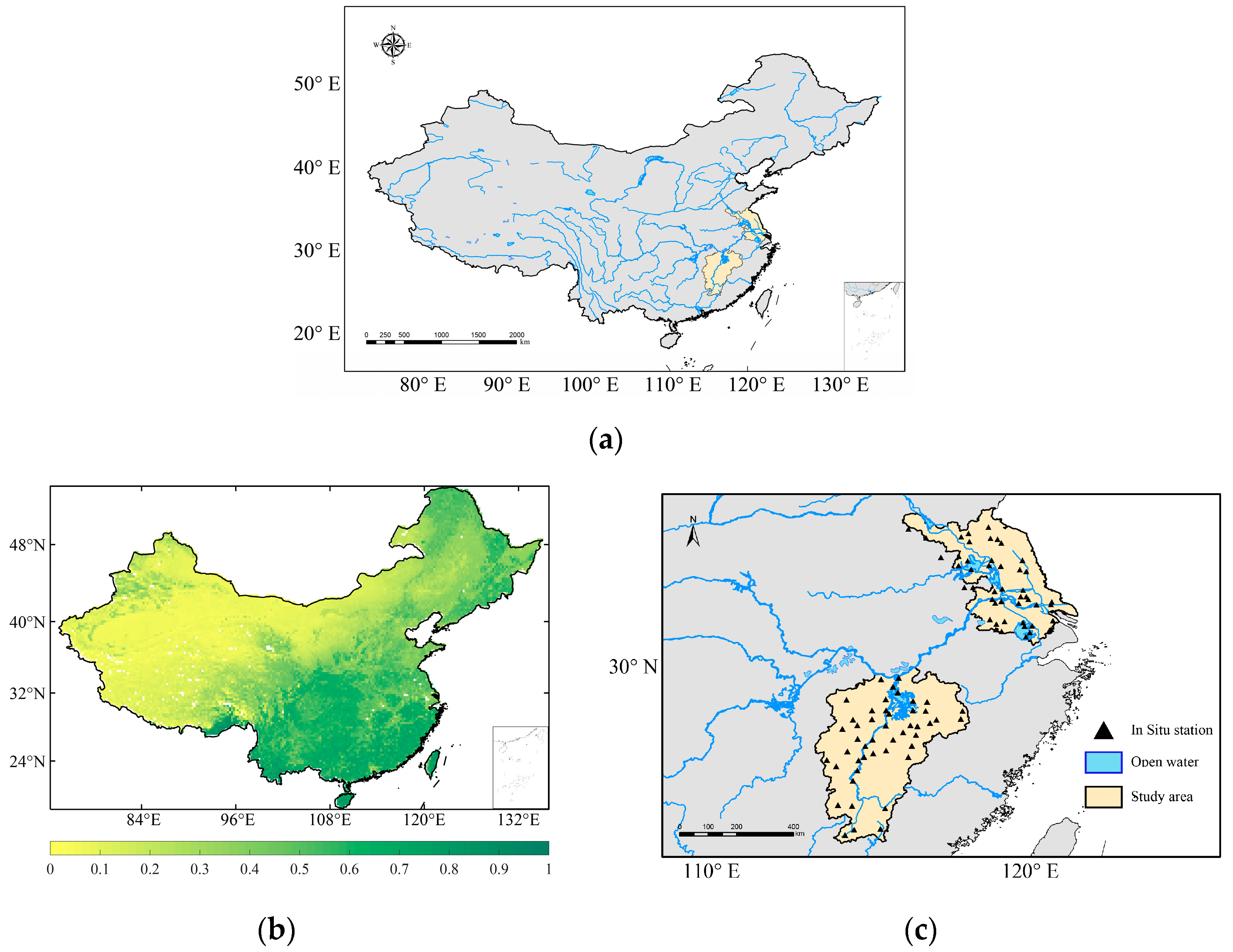
2.1. Study Area
2.2. Materials
2.2.1. FY-3B Brightness Temperature
2.2.2. ESA CCI Soil Moisture
2.2.3. GLDAS-Noah Soil Moisture
2.2.4. LPRMv5
2.2.5. LPRMv6
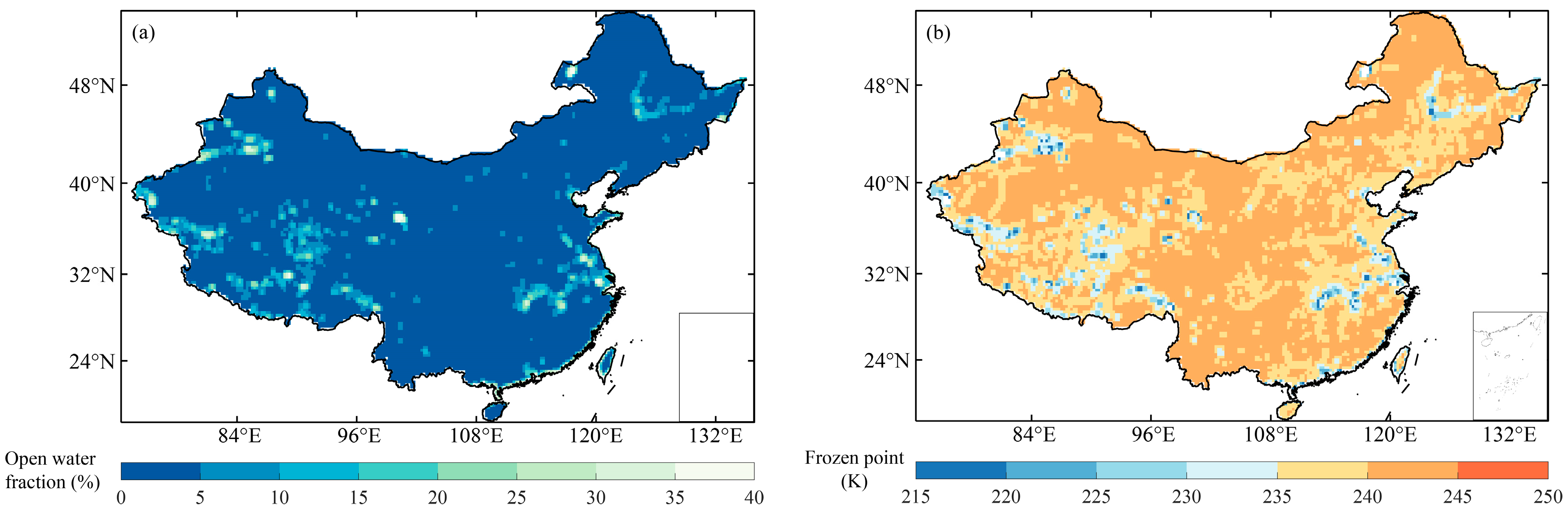
2.2.6. LPRMv6_OWF
2.2.7. LPRMv6_Veg
2.2.8. LPRMv6_OWFVeg
2.2.9. In Situ Soil Moisture
2.2.10. Normalized Difference Vegetation Index
2.3. Methodology
2.3.1. Land Parameter Retrieval Model
2.3.2. Triple Collocation Analysis
3. Results
4. Discussions
5. Conclusions
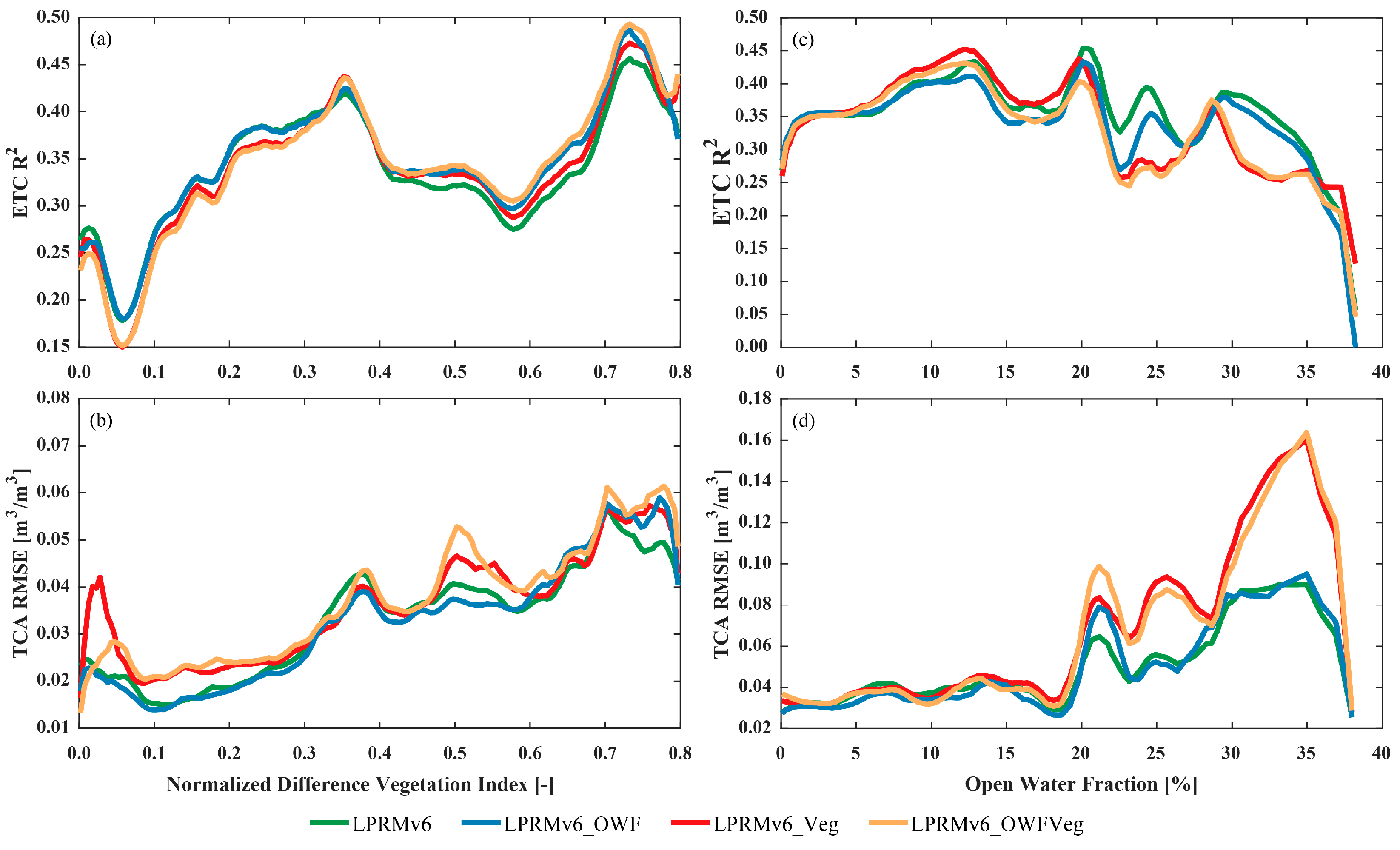
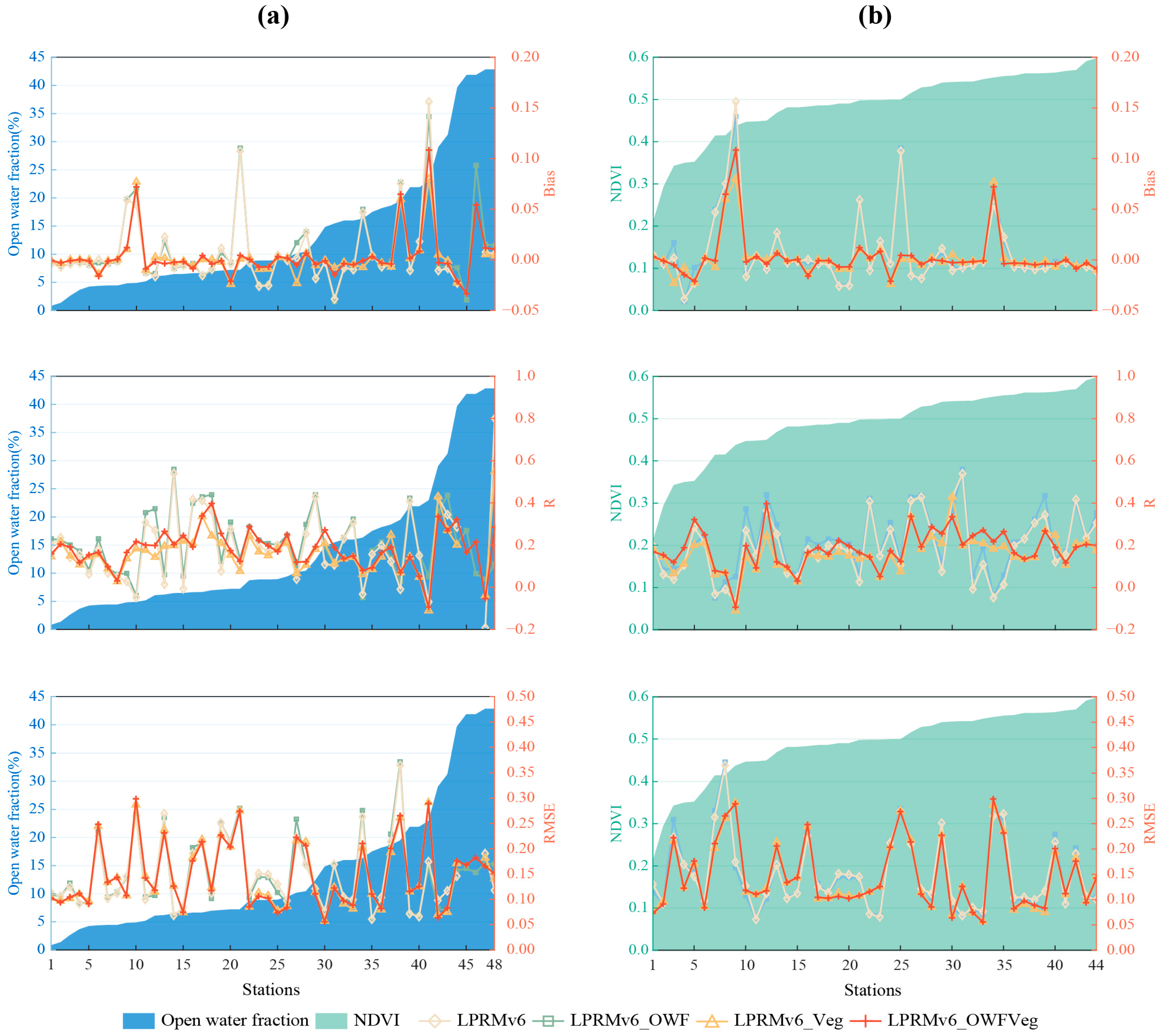
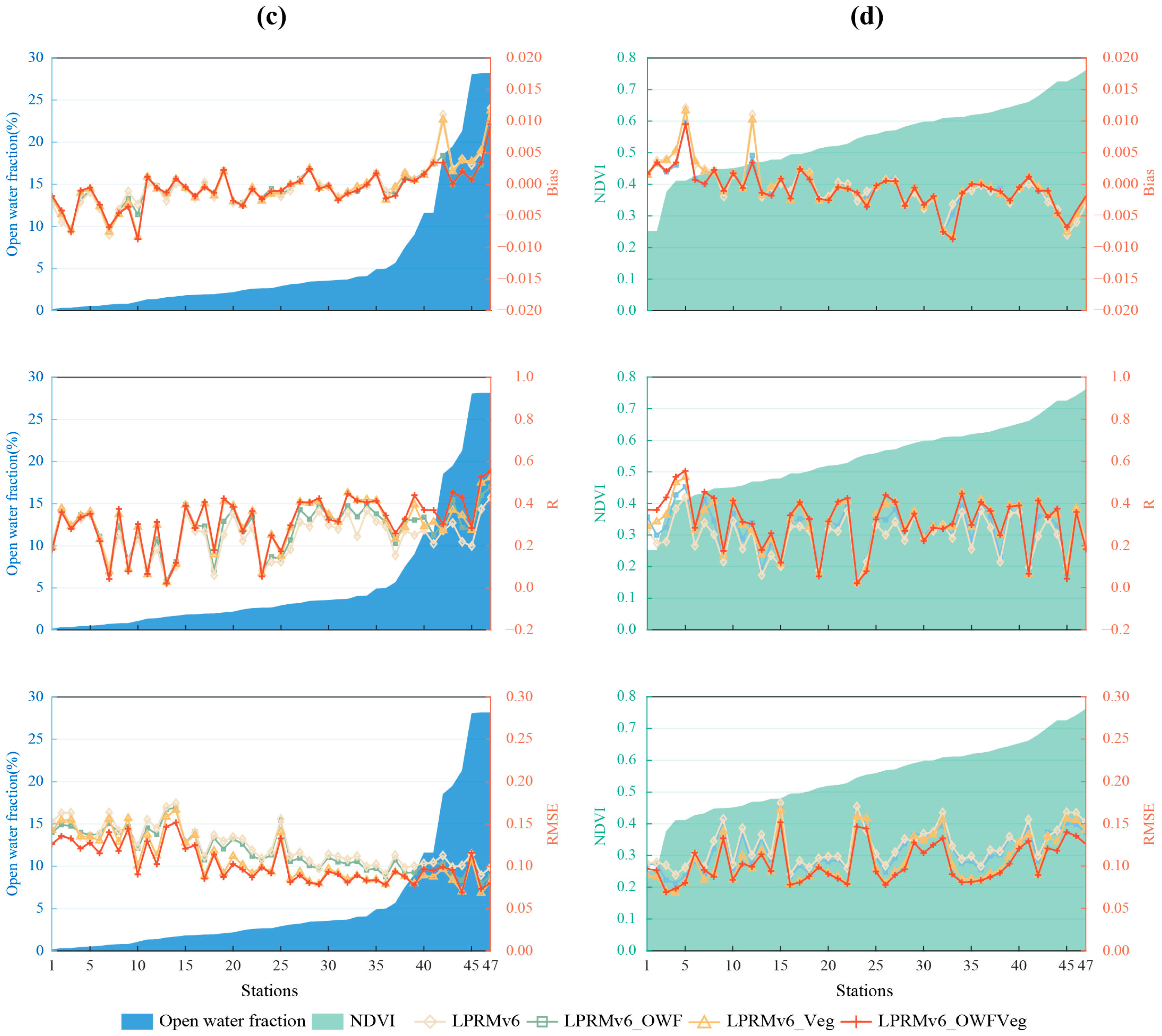
- The algorithm used to quantitatively account for the influence of open water to enhance LST inputs can improve the correlation metrics of retrieved soil-moisture data. However, when the OWF exceeds 10%, the correlation of the LPRMv6_OWF became uncertain. In comparison with the Jiangsu site, despite the significant fluctuations in the R metric, an improvement in the correlation of the LPRMv6_OWF could still be observed. Nevertheless, the performance of this approach fell short of expectations, in terms of errors.
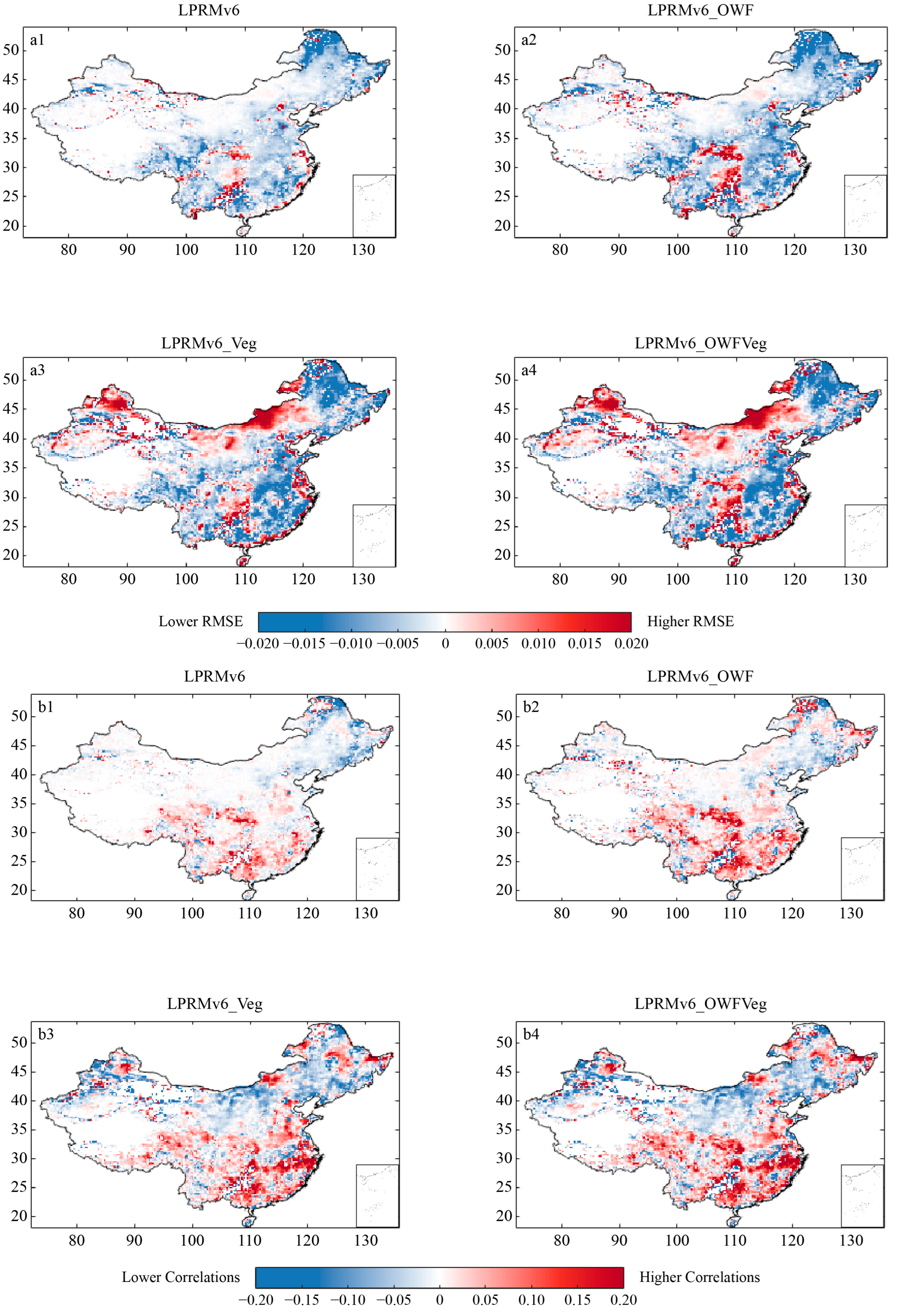
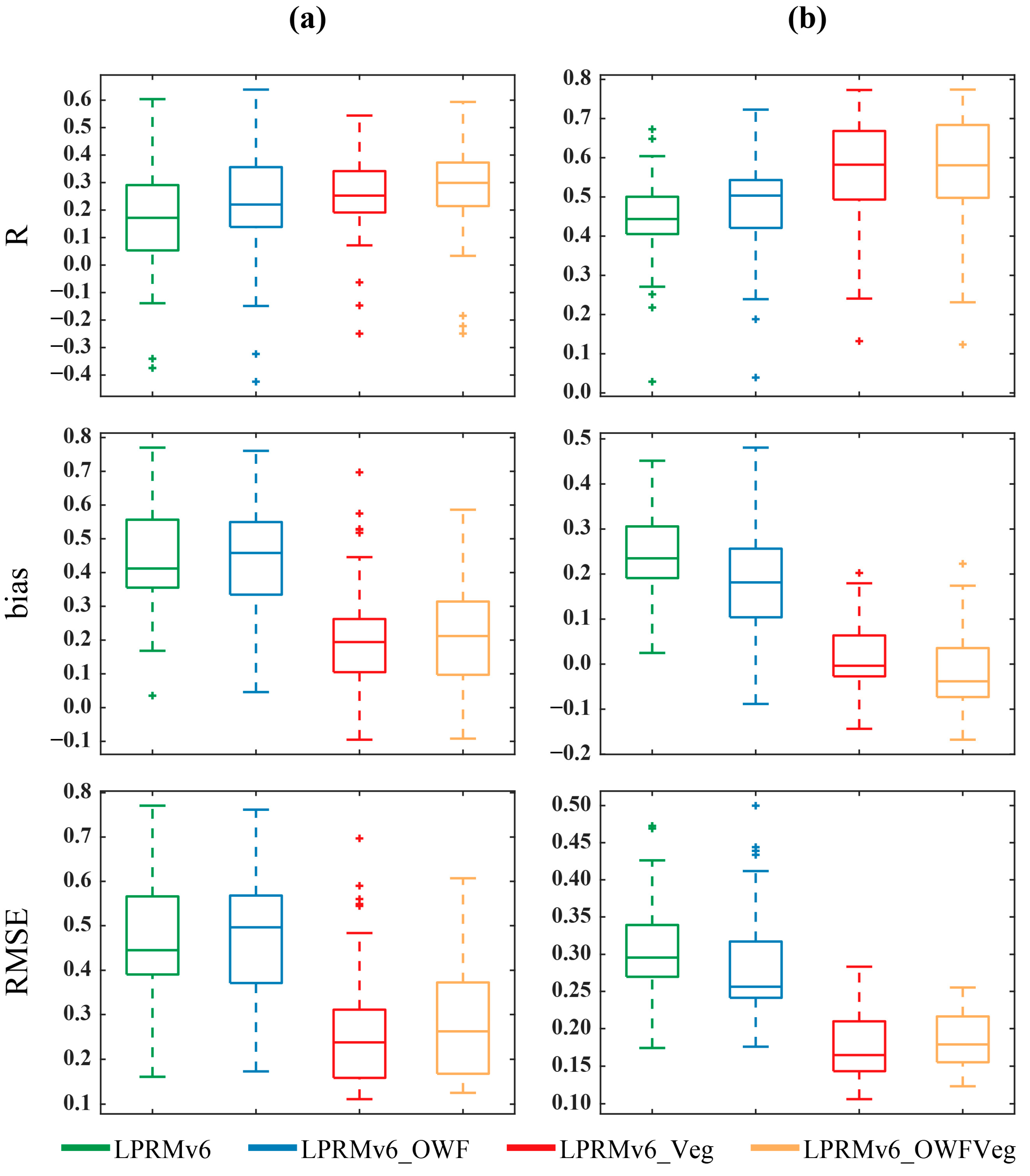
- In comparison with the Jiangxi site, the LPRMv6_Veg performed best across all metrics, primarily because its parameters were calibrated specifically for Jiangxi. However, in comparison with the Jiangsu site, considering the vegetation effects reduces data errors. Nevertheless, in the TC comparisons, both the LPRMv6_Veg and the LPRMv6_OWFVeg exhibited suboptimal performance. This suggested that a single-scattering albedo calibration, based on vegetation density conducted in Jiangxi, may not be universally applicable in the full area, as other vegetation-cover or climatic-zone effects need to be taken into account. Although in Jiangsu, the LPRMv6_Veg reduced bias and RMSE, it cannot be assumed that this algorithm is universally suitable for the Jiangsu province. This is because both Jiangsu and Jiangxi share a subtropical monsoon climate, and their vegetation exhibits certain similar characteristics.
- The LPRMv6_OWFVeg outperformed the LPRMv6_Veg in correlation, albeit the advantage was not very pronounced. However, the LPRMv6_OWFVeg exhibited notable inferiority in bias and RMSE compared to the LPRMv6_Veg. From this, we concluded that the impact of calibrating single-scattering albedo for soil-moisture retrieval based on vegetation density is more significant than the approach of enhancing LST input for soil-moisture retrieval. The LPRMv6_OWFVeg tended to perform better in regions with vegetation characteristics that were similar to Jiangxi and with an OWF below 20%.
Supplementary Materials
Author Contributions
Funding
Data Availability Statement
Acknowledgments
Conflicts of Interest
References
- Petropoulos, G.P.; Ireland, G.; Barrett, B. Surface soil moisture retrievals from remote sensing: Current status, products & future trends. Phys. Chem. Earth Parts A/B/C 2015, 83, 36–56. [Google Scholar]
- Guillod, B.P.; Orlowsky, B.; Miralles, D.G.; Teuling, A.J.; Seneviratne, S.I. Reconciling spatial and temporal soil moisture effects on afternoon rainfall. Nat. Commun. 2015, 6, 6443. [Google Scholar] [CrossRef] [PubMed]
- Orth, R.; Seneviratne, S.I. Propagation of soil moisture memory to streamflow and evapotranspiration in Europe. Hydrol. Earth Syst. Sci. 2013, 17, 3895–3911. [Google Scholar] [CrossRef]
- Seneviratne, S.I.; Corti, T.; Davin, E.L.; Hirschi, M.; Jaeger, E.B.; Lehner, I.; Orlowsky, B.; Teuling, A.J. Investigating soil moisture–climate interactions in a changing climate: A review. Earth Sci. Rev. 2010, 99, 125–161. [Google Scholar] [CrossRef]
- Wang, L.; Qu, J.J. Satellite remote sensing applications for surface soil moisture monitoring: A review. Front. Earth Sci. China 2009, 3, 237–247. [Google Scholar] [CrossRef]
- Wang, Y.; Chen, H.; Zhou, Y.; Dong, X.; Zhu, S. Subseasonal variabilities of surface soil moisture in reanalysis datasets and CESM simulations. Atmos. Ocean. Sci. Lett. 2020, 13, 34–40. [Google Scholar] [CrossRef]
- Albergel, C.; de Rosnay, P.; Gruhier, C.; Muñoz-Sabater, J.; Hasenauer, S.; Isaksen, L.; Kerr, Y.; Wagner, W. Evaluation of remotely sensed and modelled soil moisture products using global ground-based in situ observations. Remote Sens. Environ. 2012, 118, 215–226. [Google Scholar] [CrossRef]
- De Jeu, R.A.M.; Owe, M. Further validation of a new methodology for surface moisture and vegetation optical depth retrieval. Int. J. Remote Sens. 2003, 24, 4559–4578. [Google Scholar] [CrossRef]
- Fily, M.; Royer, A.; Goıta, K.; Prigent, C. A simple retrieval method for land surface temperature and fraction of water surface determination from satellite microwave brightness temperatures in sub-arctic areas. Remote Sens. Environ. 2003, 85, 328–338. [Google Scholar] [CrossRef]
- Parinussa, R.M.; de Jeu, R.A.; Holmes, T.R.; Walker, J.P. Comparison of microwave and infrared land surface temperature products over the NAFE’06 research sites. IEEE Geosci. Remote Sens. Lett. 2008, 5, 783–787. [Google Scholar] [CrossRef]
- Njoku, E.G.; Li, L. Retrieval of land surface parameters using passive microwave measurements at 6-18 GHz. IEEE Trans. Geosci. Remote Sens. 1999, 37, 79–93. [Google Scholar] [CrossRef]
- Njoku, E.G.; Wilson, W.J.; Yueh, S.H.; Dinardo, S.J.; Li, F.K.; Jackson, T.J.; Lakshmi, V.; Bolten, J. Observations of soil moisture using a passive and active low-frequency microwave airborne sensor during SGP99. IEEE Trans. Geosci. Remote Sens. 2002, 40, 2659–2673. [Google Scholar] [CrossRef]
- Owe, M.; de Jeu, R.; Walker, J. A methodology for surface soil moisture and vegetation optical depth retrieval using the microwave polarization difference index. IEEE Trans. Geosci. Remote Sens. 2001, 39, 1643–1654. [Google Scholar] [CrossRef]
- Liu, Y.Y.; Dorigo, W.A.; Parinussa, R.; de Jeu, R.A.; Wagner, W.; McCabe, M.F.; Evans, J.; Van Dijk, A. Trend-preserving blending of passive and active microwave soil moisture retrievals. Remote Sens. Environ. 2012, 123, 280–297. [Google Scholar] [CrossRef]
- Liu, Y.Y.; Parinussa, R.; Dorigo, W.A.; De Jeu, R.A.; Wagner, W.; Van Dijk, A.; McCabe, M.F.; Evans, J. Developing an improved soil moisture dataset by blending passive and active microwave satellite-based retrievals. Hydrol. Earth Syst. Sci. 2011, 15, 425–436. [Google Scholar] [CrossRef]
- Gouweleeuw, B.; Van Dijk, A.; Guerschman, J.P.; Dyce, P.; Owe, M. Space-based passive microwave soil moisture retrievals and the correction for a dynamic open water fraction. Hydrol. Earth Syst. Sci. 2012, 16, 1635–1645. [Google Scholar] [CrossRef]
- Loew, A. Impact of surface heterogeneity on surface soil moisture retrievals from passive microwave data at the regional scale: The Upper Danube case. Remote Sens. Environ. 2008, 112, 231–248. [Google Scholar] [CrossRef]
- Davenport, I.J.; Sandells, M.J.; Gurney, R.J. The effects of scene heterogeneity on soil moisture retrieval from passive microwave data. Adv. Water Resour. 2008, 31, 1494–1502. [Google Scholar] [CrossRef]
- Holmes, T.; De Jeu, R.; Owe, M.; Dolman, A. Land surface temperature from Ka band (37 GHz) passive microwave observations. J. Geophys. Res. Atmos. 2009, 114, D04113. [Google Scholar] [CrossRef]
- Mladenova, I.; Jackson, T.; Njoku, E.; Bindlish, R.; Chan, S.; Cosh, M.; Holmes, T.; De Jeu, R.; Jones, L.; Kimball, J. Remote monitoring of soil moisture using passive microwave-based techniques—Theoretical basis and overview of selected algorithms for AMSR-E. Remote Sens. Environ. 2014, 144, 197–213. [Google Scholar] [CrossRef]
- Moran, M.S.; Peters-Lidard, C.D.; Watts, J.M.; McElroy, S. Estimating soil moisture at the watershed scale with satellite-based radar and land surface models. Can. J. Remote Sens. 2004, 30, 805–826. [Google Scholar] [CrossRef]
- Parinussa, R.M.; De Jeu, R.A.; Van der Schalie, R.; Crow, W.T.; Lei, F.; Holmes, T.R. A quasi-global approach to improve day-time satellite surface soil moisture anomalies through the land surface temperature input. Climate 2016, 4, 50. [Google Scholar] [CrossRef]
- Van der Schalie, R.; de Jeu, R.A.; Kerr, Y.H.; Wigneron, J.-P.; Rodríguez-Fernández, N.J.; Al-Yaari, A.; Parinussa, R.M.; Mecklenburg, S.; Drusch, M. The merging of radiative transfer based surface soil moisture data from SMOS and AMSR-E. Remote Sens. Environ. 2017, 189, 180–193. [Google Scholar] [CrossRef]
- Parinussa, R.M.; Wang, G.; Liu, Y.; Lou, D.; Hagan, D.F.T.; Zhan, M.; Su, B.; Jiang, T. Improved surface soil moisture anomalies from Fengyun-3B over the Jiangxi province of the People’s Republic of China. Int. J. Remote Sens. 2018, 39, 8950–8962. [Google Scholar] [CrossRef]
- Song, P.; Huang, J.; Mansaray, L.R.; Wen, H.; Wu, H.; Liu, Z.; Wang, X. An Improved Soil Moisture Retrieval Algorithm Based on the Land Parameter Retrieval Model for Water–Land Mixed Pixels Using AMSR-E Data. IEEE Trans. Geosci. Remote Sens. 2019, 57, 7643–7657. [Google Scholar] [CrossRef]
- Parinussa, R.; Holmes, T.; Yilmaz, M.; Crow, W. The impact of land surface temperature on soil moisture anomaly detection from passive microwave observations. Hydrol. Earth Syst. Sci. 2011, 15, 3135–3151. [Google Scholar] [CrossRef]
- Hagan, D.F.; Wang, G.; Parinussa, R.; Shi, X. Inter-comparing and improving land surface temperature estimates from passive microwaves over the Jiangsu province of the People’s Republic of China. Int. J. Remote Sens. 2019, 40, 5563–5584. [Google Scholar] [CrossRef]
- Hagan, D.F.T.; Parinussa, R.M.; Wang, G.; Draper, C.S. An evaluation of soil moisture anomalies from global model-based datasets over the people’s republic of China. Water 2019, 12, 117. [Google Scholar] [CrossRef]
- Dorigo, W.; Wagner, W.; Albergel, C.; Albrecht, F.; Balsamo, G.; Brocca, L.; Chung, D.; Ertl, M.; Forkel, M.; Gruber, A. ESA CCI Soil Moisture for improved Earth system understanding: State-of-the art and future directions. Remote Sens. Environ. 2017, 203, 185–215. [Google Scholar]
- Wang, G.; Ma, X.; Hagan, D.F.T.; van der Schalie, R.; Kattel, G.; Ullah, W.; Tao, L.; Miao, L.; Liu, Y. Towards Consistent Soil Moisture Records from China’s FengYun-3 Microwave Observations. Remote Sens. 2022, 14, 1225. [Google Scholar] [CrossRef]
- Wu, Z.; Feng, H.; He, H.; Zhou, J.; Zhang, Y. Evaluation of soil moisture climatology and anomaly components derived from ERA5-land and GLDAS-2.1 in China. Water Resour. Manag. 2021, 35, 629–643. [Google Scholar] [CrossRef]
- Liu, Y.; Liu, Y.; Wang, W. Inter-comparison of satellite-retrieved and Global Land Data Assimilation System-simulated soil moisture datasets for global drought analysis. Remote Sens. Environ. 2019, 220, 1–18. [Google Scholar] [CrossRef]
- van der Schalie, R.; Kerr, Y.H.; Wigneron, J.-P.; Rodríguez-Fernández, N.J.; Al-Yaari, A.; de Jeu, R.A. Global SMOS soil moisture retrievals from the land parameter retrieval model. Int. J. Appl. Earth Obs. Geoinf. 2016, 45, 125–134. [Google Scholar]
- Crow, W.T.; Berg, A.A.; Cosh, M.H.; Loew, A.; Mohanty, B.P.; Panciera, R.; de Rosnay, P.; Ryu, D.; Walker, J.P. Upscaling sparse ground-based soil moisture observations for the validation of coarse-resolution satellite soil moisture products. Rev. Geophys. 2012, 50, RG2002. [Google Scholar] [CrossRef]
- Drusch, M.; Wood, E.F.; Jackson, T.J. Vegetative and atmospheric corrections for the soil moisture retrieval from passive microwave remote sensing data: Results from the Southern Great Plains Hydrology Experiment 1997. J. Hydrometeorol. 2001, 2, 181–192. [Google Scholar] [CrossRef]
- Reichle, R.H.; Koster, R.D.; Dong, J.; Berg, A.A. Global soil moisture from satellite observations, land surface models, and ground data: Implications for data assimilation. J. Hydrometeorol. 2004, 5, 430–442. [Google Scholar] [CrossRef]
- Wagner, W.; Blöschl, G.; Pampaloni, P.; Calvet, J.-C.; Bizzarri, B.; Wigneron, J.-P.; Kerr, Y. Operational readiness of microwave remote sensing of soil moisture for hydrologic applications. Hydrol. Res. 2007, 38, 1–20. [Google Scholar] [CrossRef]
- De Jeu, R.A.; Wagner, W.; Holmes, T.; Dolman, A.; Van De Giesen, N.; Friesen, J. Global soil moisture patterns observed by space borne microwave radiometers and scatterometers. Surv. Geophys. 2008, 29, 399–420. [Google Scholar] [CrossRef]
- Meesters, A.G.; De Jeu, R.A.; Owe, M. Analytical derivation of the vegetation optical depth from the microwave polarization difference index. IEEE Geosci. Remote Sens. Lett. 2005, 2, 121–123. [Google Scholar] [CrossRef]
- Owe, M.; de Jeu, R.; Holmes, T. Multisensor historical climatology of satellite-derived global land surface moisture. J. Geophys. Res. Earth Surf. 2008, 113, F01002. [Google Scholar] [CrossRef]
- Wigneron, J.-P.; Kerr, Y.; Waldteufel, P.; Saleh, K.; Escorihuela, M.-J.; Richaume, P.; Ferrazzoli, P.; De Rosnay, P.; Gurney, R.; Calvet, J.-C. L-band Microwave Emission of the Biosphere (L-MEB) Model: Description and calibration against experimental data sets over crop fields. Remote Sens. Environ. 2007, 107, 639–655. [Google Scholar] [CrossRef]
- Parinussa, R.M.; Holmes, T.R.; de Jeu, R.A. Soil moisture retrievals from the WindSat spaceborne polarimetric microwave radiometer. IEEE Trans. Geosci. Remote Sens. 2011, 50, 2683–2694. [Google Scholar] [CrossRef]
- Dorigo, W.; Xaver, A.; Vreugdenhil, M.; Gruber, A.; Hegyiova, A.; Sanchis-Dufau, A.; Zamojski, D.; Cordes, C.; Wagner, W.; Drusch, M. Global automated quality control of in situ soil moisture data from the International Soil Moisture Network. Vadose Zone J. 2013, 12, 1–21. [Google Scholar] [CrossRef]
- Yilmaz, M.T.; Crow, W.T. Evaluation of assumptions in soil moisture triple collocation analysis. J. Hydrometeorol. 2014, 15, 1293–1302. [Google Scholar] [CrossRef]
- McColl, K.A.; Vogelzang, J.; Konings, A.G.; Entekhabi, D.; Piles, M.; Stoffelen, A. Extended triple collocation: Estimating errors and correlation coefficients with respect to an unknown target. Geophys. Res. Lett. 2014, 41, 6229–6236. [Google Scholar] [CrossRef]
- Draper, C.; Reichle, R.; de Jeu, R.; Naeimi, V.; Parinussa, R.; Wagner, W. Estimating root mean square errors in remotely sensed soil moisture over continental scale domains. Remote Sens. Environ. 2013, 137, 288–298. [Google Scholar] [CrossRef]
- Parinussa, R.M.; Wang, G.; Liu, Y.Y.; Hagan, D.F.; Lin, F.; Van der Schalie, R.; De Jeu, R.A. The Evaluation of Single-Sensor Surface Soil Moisture Anomalies over the Mainland of the People’s Republic of China. Remote Sens. 2017, 9, 149. [Google Scholar] [CrossRef]
- McColl, K.A.; Roy, A.; Derksen, C.; Konings, A.G.; Alemohammed, S.H.; Entekhabi, D. Triple collocation for binary and categorical variables: Application to validating landscape freeze/thaw retrievals. Remote Sens. Environ. 2016, 176, 31–42. [Google Scholar] [CrossRef]
- Pan, M.; Fisher, C.K.; Chaney, N.W.; Zhan, W.; Crow, W.T.; Aires, F.; Entekhabi, D.; Wood, E.F. Triple collocation: Beyond three estimates and separation of structural/non-structural errors. Remote Sens. Environ. 2015, 171, 299–310. [Google Scholar] [CrossRef]
- Lei, F.; Crow, W.T.; Shen, H.; Parinussa, R.M.; Holmes, T.R. The impact of local acquisition time on the accuracy of microwave surface soil moisture retrievals over the contiguous United States. Remote Sens. 2015, 7, 13448–13465. [Google Scholar] [CrossRef]
- Scipal, K.; Dorigo, W.; deJeu, R. Triple collocation—A new tool to determine the error structure of global soil moisture products. In Proceedings of the 2010 IEEE International Geoscience and Remote Sensing Symposium, Honolulu, HI, USA, 25–30 July 2010; pp. 4426–4429. [Google Scholar]
- Gruber, A.; Su, C.-H.; Zwieback, S.; Crow, W.; Dorigo, W.; Wagner, W. Recent advances in (soil moisture) triple collocation analysis. Int. J. Appl. Earth Obs. Geoinf. 2016, 45, 200–211. [Google Scholar] [CrossRef]


| Data Types | Data/Scheme | Land-Surface Temperature | Single-Scattering Albedo | Roughness Parameter | Spatial Resolution | Time Resolution | Source |
|---|---|---|---|---|---|---|---|
| Source data | Brightness temperature | / | / | / | 0.25° | Descending | National Satellite Meteorological Centre, FunYun-3B |
| Comparative data | LPRMv5 | H09 | Global constant | Global constant | 0.25° | Descending | Holmes et al. [19] |
| LPRMv6 | H09 | SMOS-calibrated | SMOS-calibrated | 0.25° | Descending | Van der Schalie et al. [23] | |
| LPRMv6_OWF | HG19 | SMOS-calibrated | SMOS-calibrated | 0.25° | Descending | Hagan et al. [27] | |
| LPRMv6_Veg | H09 | Vegetation-density-based | SMOS-calibrated | 0.25° | Descending | Parinussa et al. [24] | |
| LPRMv6_OWFVeg | HG19 | Vegetation-density-based | SMOS-calibrated | 0.25° | Descending | This paper | |
| Validation data | ESA CCI soil moisture | / | / | / | 0.25° | Daily | ESA, CCI |
| GLDAS-Noah soil moisture | / | / | / | 0.25° | Hourly | NASA and NCEP | |
| In situ soil moisture | / | / | / | / | Hourly | Jiangsu and Jiangxi Meteorological Information Centers | |
| Ancillary data | NDVI | / | / | / | 0.05° | Monthly | MODIS |
| Land cover dataset | / | / | / | 800 m | / | Institute of Geographical Sciences and Natural Resources Research of the Chinese Academy of Sciences |
Disclaimer/Publisher’s Note: The statements, opinions and data contained in all publications are solely those of the individual author(s) and contributor(s) and not of MDPI and/or the editor(s). MDPI and/or the editor(s) disclaim responsibility for any injury to people or property resulting from any ideas, methods, instructions or products referred to in the content. |
© 2023 by the authors. Licensee MDPI, Basel, Switzerland. This article is an open access article distributed under the terms and conditions of the Creative Commons Attribution (CC BY) license (https://creativecommons.org/licenses/by/4.0/).
Share and Cite
Liu, H.; Wang, G.; Hagan, D.F.T.; Hu, Y.; Nooni, I.K.; Yeboah, E.; Zhou, F. Evaluation of Improvement Schemes for FY-3B Passive Microwave Soil-Moisture Estimates Retrieved Using the Land Parameter Retrieval Model. Remote Sens. 2023, 15, 5108. https://doi.org/10.3390/rs15215108
Liu H, Wang G, Hagan DFT, Hu Y, Nooni IK, Yeboah E, Zhou F. Evaluation of Improvement Schemes for FY-3B Passive Microwave Soil-Moisture Estimates Retrieved Using the Land Parameter Retrieval Model. Remote Sensing. 2023; 15(21):5108. https://doi.org/10.3390/rs15215108
Chicago/Turabian StyleLiu, Haonan, Guojie Wang, Daniel Fiifi Tawia Hagan, Yifan Hu, Isaac Kwesi Nooni, Emmanuel Yeboah, and Feihong Zhou. 2023. "Evaluation of Improvement Schemes for FY-3B Passive Microwave Soil-Moisture Estimates Retrieved Using the Land Parameter Retrieval Model" Remote Sensing 15, no. 21: 5108. https://doi.org/10.3390/rs15215108