
Spatial Downscaling of Near-Surface Air Temperature Based on Deep Learning Cross-Attention Mechanism


1
School of Geographical Sciences, Nanjing University of Information Science and Technology, Nanjing 210044, China
2
National Meteorological Information Center, Beijing 100044, China
3
Institute of Aerospace Information, Space Engineering University, Beijing 101400, China
*
Author to whom correspondence should be addressed.
Remote Sens. 2023, 15(21), 5084; https://doi.org/10.3390/rs15215084
Submission received: 23 August 2023
/
Revised: 11 October 2023
/
Accepted: 14 October 2023
/
Published: 24 October 2023
(This article belongs to the Special Issue Advances in Deep Learning in the Retrieval of Key Parameters of Agrometeorological Remote Sensing)
Abstract
:Deep learning methods can achieve a finer refinement required for downscaling meteorological elements, but their performance in terms of bias still lags behind physical methods. This paper proposes a statistical downscaling network based on Light-CLDASSD that utilizes a Shuffle–nonlinear-activation-free block (SNBlock) and Swin cross-attention mechanism (SCAM), and is named SNCA-CLDASSD, for the China Meteorological Administration Land Data Assimilation System (CLDAS). This method aims to achieve a more accurate spatial downscaling of a temperature product from 0.05° to 0.01° for the CLDAS. To better utilize the digital elevation model (DEM) for reconstructing the spatial texture of the temperature field, a module named SCAM is introduced, which can activate more input pixels and enable the network to correct and merge the extracted feature maps with DEM information. We chose 90% of the CLDAS temperature data with DEM and station observation data from 2016 to 2020 (excluding 2018) as the training set, 10% as the verification set, and chose the data in 2018 as the test set. We validated the effectiveness of each module through comparative experiments and obtained the best-performing model. Then, we compared it with traditional interpolation methods and state-of-the-art deep learning super-resolution algorithms. We evaluated the experimental results with HRCLDAS, national stations, and regional stations, and the results show that our improved model performs optimally compared to other methods (RMSE of 0.71 °C/0.12 °C/0.72 °C, BIAS of −0.02 °C/0.02 °C/0.002 °C), with the most noticeable improvement in mountainous regions, followed by plains. SNCA-CLDASSDexhibits the most stable performance in intraday hourly bias at temperature under the conditions of improved feature extraction capability in the SNBlock and a better utilization of the DEM by the SCAM. Due to the replacement of the upsampling method from sub pixels to CARAFE, it effectively suppresses the checkerboard effect and shows better robustness than other models. Our approach extends the downscaling model for CLDAS data products and significantly improves performance in this task by enhancing the model’s feature extraction and fusion capabilities and improving upsampling methods. It offers a more profound exploration of historical high-resolution temperature estimation and can be migrated to the downscaling of other meteorological elements.
1. Introduction
The High-Resolution China Meteorological Administration Land Data Assimilation System (HRCLDAS) [1] relies on a large amount of dense ground observation data to produce high-resolution and high-quality assimilation products. Due to the sparse number of national meteorological stations before 2008, there is a lack of high-coverage ground observation data. Therefore, relying solely on existing observational data makes it challenging for the HRCLDAS to retrieve high-quality, high-resolution land surface data before 2008. Downscaling techniques can effectively address such issues. Low-resolution meteorological and auxiliary data can be used to generate high-resolution meteorological data, enabling a small-scale reconstruction of local information. Downscaling methods are mainly divided into two categories: dynamic downscaling and statistical downscaling.
The dynamical downscaling method nests a regionally limited climate model (RCM) within a global climate model (GCM). It utilizes the initial boundary conditions provided by the GCM to obtain high-resolution weather information after numerically integrating the regional climate model. Huang et al. [2] evaluate VR-CESM for California’s climate using high-resolution data, comparing it to observational and RCM data (WRF), and the results suggest its potential in fine-scale climate modeling. Chen et al. [3] improve regional climate simulations by nesting CWRF within ECHAM, leading to better temperature and precipitation predictions over the contiguous US. These methods utilize various dynamic and thermodynamic processes, independent of observational data, with a strong mathematical and physical foundation. However, dynamic downscaling models exhibit notable systematic biases in climate simulations [4]. In comparison to dynamic downscaling, statistical downscaling offers relative simplicity, reduced computational time requirements, and greater flexibility of implementation strategies in the study area, and it has been widely applied in regional climate simulation. Statistical downscaling methods can be classified into three categories: transfer function methods [5,6], weather pattern methods [7,8], and stochastic weather generators [9,10].
In recent years, the rise of deep learning technology has provided new insights for further improving the accuracy of statistical downscaling results. Among them, image super-resolution techniques have emerged as important image reconstruction methods in computer vision. Their objective is to restore high-resolution images from low-resolution counterparts. The methods are widely applied in diverse fields such as remote sensing, video restoration, 3D rendering et al. [11,12,13,14]. Image super-resolution and statistical downscaling are well-matched, and both natural images and meteorological features can be described using digital matrices. Increasingly, research has demonstrated that end-to-end image super-resolution algorithms can be effectively migrated to meteorological element downscaling to improve the accuracy [15,16,17]. However, the distinctions between meteorological data and natural images, such as the number of data channels, the coupling degree, and the inherent relationships between high and low-resolution data, impose limitations on their application. These distinctions should be taken into account when constructing downscaling models.
In 2017, Vandal et al. [18] introduced DeepSD, a super-resolution-based downscaling method, which broke down high-magnification downscaling into smaller tasks using a stacked SRCNN structure. It outperformed traditional methods for the precipitation over the US. In 2019, Mao [19] improved DeepSD with VDSD and ResSD models, effectively addressing network depth and non-integer scaling limitations. These models excelled in the precipitation in China, surpassing DeepSD in TS score. In the same year, Singh et al. [20] applied generative adversarial networks (GANs) to downscaling, improving wind field reconstruction using ESRGAN, outperforming bicubic interpolation and SRCNN. In 2020, Höhlein et al. [21] developed DeepRU, utilizing the UNet architecture to efficiently reconstruct wind field structures, overcoming issues faced by traditional CNN algorithms. In 2022, Gerges et al. [22] introduced AIG-Transformer, transforming spatial downscaling into a multivariate time-series prediction task, outperforming existing methods for weekly temperatures. Also, Tie et al. [23] enhanced VDSD to create CLDASSD with global skip connections and attention mechanisms, exhibiting strong spatial reconstruction in complex terrains. Light-CLDASSD [24], an improved version in the same year, captured distribution characteristics of small-scale temperature field in plain areas.
However, in the above works, researchers focused on incorporating high-resolution auxiliary data such as the DEM to enhance model performance without effectively extracting feature information from these auxiliary data. Therefore, this paper addresses the challenge of better utilizing high-resolution auxiliary data and proposes the Shuffle–nonlinear-activation-free module and Swin cross-attention-mechanism-based CLDAS statistical downscaling model (SNCA-CLDASSD). To better reconstruct the temperature field, this study primarily focuses on three points: (1) Capturing the intrinsic connection between temperature data of different resolutions; (2) leveraging DEM data to analyze their influence on the temperature field and learning the relationships between them; (3) selecting an effective upsampling algorithm for deep learning network models that directly influences the result generation.
In response to these points, our main contributions can be summarized as follows:
- Without increasing the number of parameters and computational complexity of the network, we introduce the feature extraction module of SNBlock to augment the network’s feature extraction capability and the mapping learning ability between high and low-resolution temperature fields.
- Replacing the upsampling operator from sub-pixel to CARAFE, which is lightweight and has a larger receptive field to reconstruct spatial details, effectively mitigates the occurrence of checkerboard artifacts.
2. Materials and Methods
2.1. Study Area and Data
2.1.1. Study Area
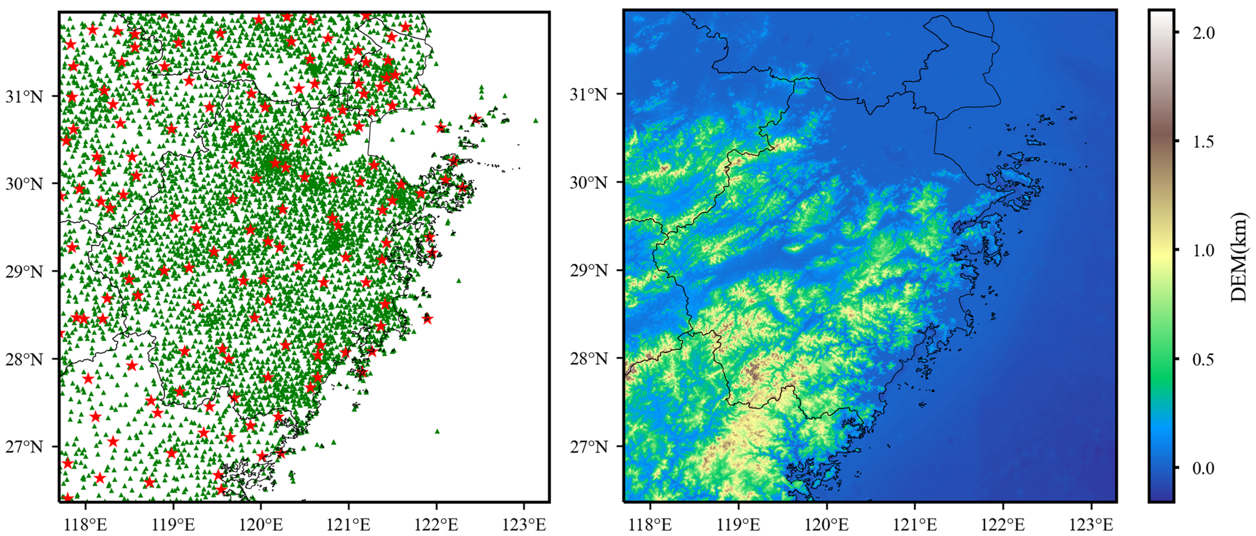
The study area of this paper spans from 117.7°E to 123.3°E in longitude and from 26.35°N to 31.95°N in latitude, encompassing the regions of Zhejiang, Fujian, Jiangsu, Anhui, Jiangxi, Shanghai, and their surrounding areas. As depicted in Figure 1, the eastern and western parts of the study area consist of ocean and land, respectively. The northern region of the study area is primarily the middle and lower reaches of the Yangtze River plain, the central part is Jiangnan hilly regions, and the southern area comprises the Wuyi Mountains, resulting in a complex topography. Influenced by monsoons, the region experiences a subtropical monsoon climate with ample sunshine throughout the year, abundant rainfall, synchronous seasonal changes between rainy and hot periods, and a diverse distribution of climate resources. This area is susceptible to a variety of meteorological disasters due to its complex climatic conditions.
2.1.2. Data
The low-resolution (0.05°) land surface data are from the CLDAS-V2.0 product generated by the National Meteorological Information Center of the China Meteorological Administration. This product covers the Asian region (0–60°N, 70–140°E) and provides hourly fused grid data of land–atmosphere interactions. The data have a spatial resolution of 0.05° in an equal latitude–longitude projection [27]. The CLDAS product incorporates various ground and satellite observation data and techniques, such as space-time multiscale analysis system (STMAS), cumulative distribution function (CDF) matching, physical inversion, and terrain correction. When compared with similar products both domestically and internationally, the CLDAS product demonstrates superior quality. Each low-resolution temperature field within the study area has a size of 112 × 112.
The high-resolution (0.01°) label data are from the HRCLDAS-V1.0 product and provide hourly fused grid land surface data with a spatial resolution of 0.01° in an equal latitude–longitude projection. The temperature, pressure, humidity, and wind products of HRCLDAS employ the STMAS to assimilate ECMWF products along with data from over 60,000 national and regional automatic meteorological stations deployed by the China Meteorological Administration. Each high-resolution temperature field label within the study area has a size of 560 × 560.
The 0.01° DEM data are from the joint mapping efforts of NASA and national space agencies of the United States, Germany, and Italy under the Shuttle Radar Topography Mission (SRTM). The current version, SRTM V4.1, is interpolated using a new algorithm developed by the International Center for Tropical Agriculture (CIAT) to fill data gaps effectively [28]. The DEM data for the study area also have a size of 560 × 560.
The study area consists of 157 national automatic meteorological stations and 5829 regional automatic meteorological stations. The spatial distribution of observation stations is shown in Figure 1.
All the data used in this study are detailed in Table 1. For the training phase, 90% of the hourly data from the years 2016, 2017, 2019, and 2020 are allocated for training, 10% for validation, and the year 2018 is used as an independent test set. The sample sizes of the three datasets are 25,602, 2845, and 8760, respectively. During the training stage, the DEM is introduced as auxiliary data, and a loss function is constructed using station observation data to enforce soft constraints on the model, improving network accuracy.
2.2. Data Preprocessing
Although the 0.05° and 0.01° resolutions are the same in spatial sampling, there exists systematic error between the two types of products (low-resolution data from CLDAS and high-resolution data from HRCLDAS). Additionally, the data from the national meteorological stations of the China Meteorological Administration are stable and reliable, requiring no data cleaning. However, the regional stations often exhibit data instability and large errors, necessitating data-cleaning procedures.
To enable the model to learn a better spatial mapping relationship, this paper adopts the following data-cleaning measures.
2.2.1. Grid Data
According to the provisions on climatic threshold values for temperature elements in the ground-based meteorological observation data quality control, as stipulated in the Meteorological Industry Standard of China (QX/T 118-2020) [29], data pairs with temperature values within the range of −80 °C to 60 °C should be retained. Data pairs within the ±3 confidence interval of the residual distribution between high-resolution and low-resolution data should also be retained. Ultimately, all data need to be validated manually.
2.2.2. Regional Stations Data
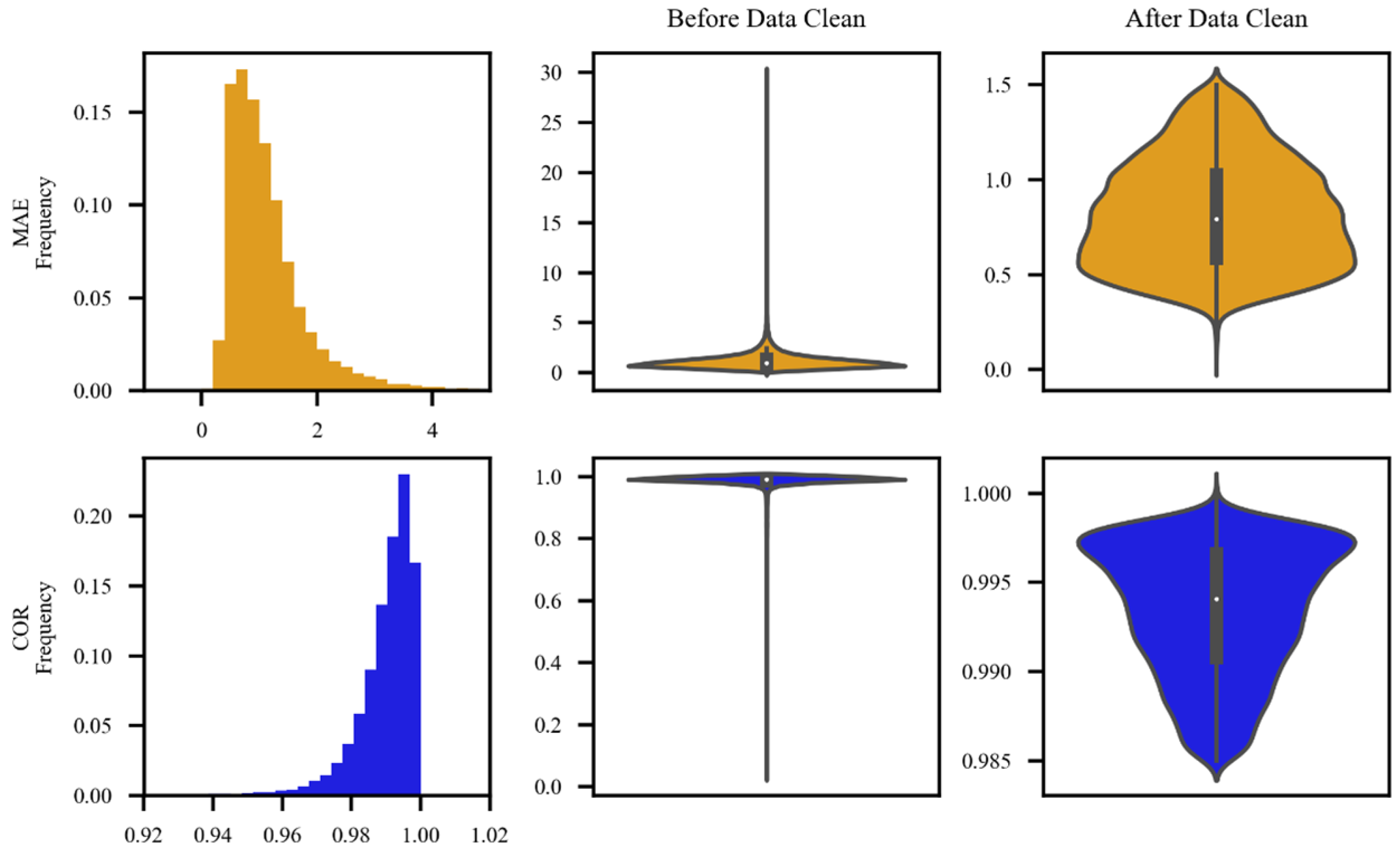
Following the stipulations regarding climatic threshold values for temperature elements in ground-based meteorological observation data quality control as outlined in the Meteorological Industry Standard of China (QX/T 118-2020) [29], data pairs with temperature values falling within the range of −80 °C to 60 °C are to be retained. A comparison and computation of regional station data with CLDAS data yield statistical results for mean absolute error (MAE) and correlation coefficient (COR), as presented in rows 1 and 2 of Figure 2. According to the statistical outcomes, it is evident that, before data cleaning, MAE values for regional station data versus CLDAS data exhibit a distribution ranging from 0 to 30, with a predominant concentration from 0 to 4. Similarly, COR values are distributed between 0 and 1, with a predominant concentration from 0.96 to 1. Based on the aforementioned statistical results, this study retains regional station data with MAE and COR values occurring with a frequency distribution of 0.05 or above. As revealed in column 3 of Figure 2, following the data cleaning, it is possible to maintain MAE and COR within a reasonable range, thereby eliminating a majority of outliers.
2.3. SNCA-CLDASSD
This study presents an enhancement to the architecture of Light-CLDASSD, which is a statistical downscaling network model for the CLDAS temperature data, referred to as SNCA-CLDASSD, based on shuffling-nonlinear-activation-free block (SNBlock) and Swin cross-attention mechanism (SCAM). Light-CLDASSD is a lightweight model upgrade developed by Tie et al. [24] to address issues such as excessive parameterization, low computational efficiency, and limited accuracy in regional downscaling at sites of CLDASSD. However, this model still exhibits deficiencies in downscaling accuracy for plain areas, notable artifacts like the checkerboard effect, and is constrained by a relatively small training dataset (four daily time steps per day in 2019), significantly impacting its generalization capability. Therefore, this paper introduces the SNCA-CLDASSD model to mitigate these shortcomings.
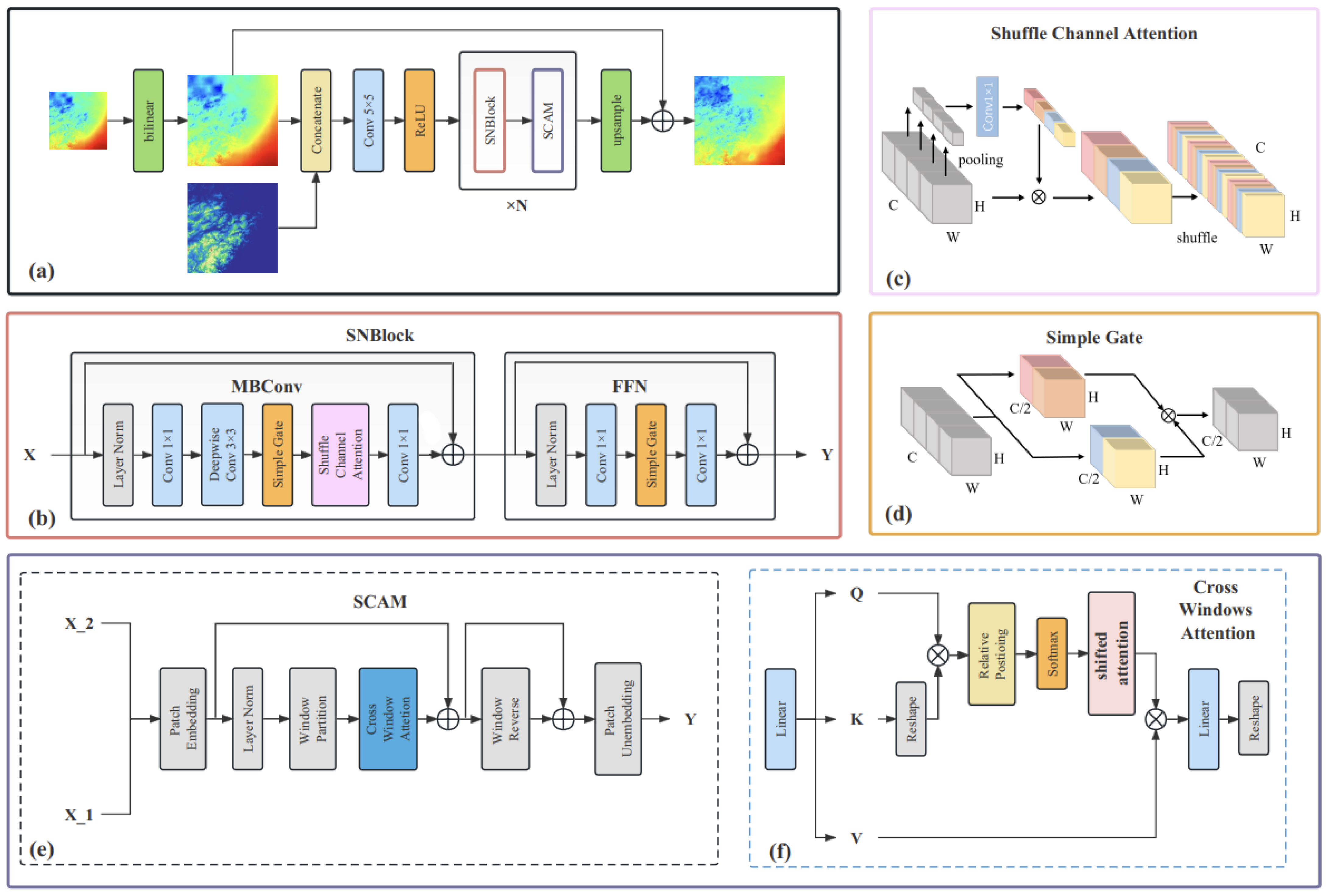
SNCA-CLDASSD employs a commonly used encoder–decoder structure in deep learning, primarily composed of Shuffle–nonlinear-activation-free block (SNBlock), Swin cross-attention mechanism (SCAM), and upsampling modules. The SNBlock serves as the principal feature extraction component of the model, while the SCAM better learns and extracts spatial features from high-resolution auxiliary data, such as DEM. The SNBlock and SCAM together constitute the main feature extraction framework of the model, iteratively repeated N times to enhance the model’s spatial reconstruction capability. When N is even, SCAM is concatenated after SNBlock; when N is odd, SCAM is not added. Simultaneously, following the concept of residual learning [30], the bilinear-interpolated temperature field is added to the upsampled temperature field, facilitating the learning of global residuals. The overall model structure is illustrated in Figure 3a, and each module depicted in the figure will be elaborated upon in the subsequent sections.
2.4. Shuffle–Nonlinear-Activation-Free Block
The design of the Shuffle–nonlinear-activation-free Block (SNBlock) originates from both ShuffleNet [31] and NAFNet [32], as depicted in Figure 3b. This module can be decomposed into two components: (1) The mobile convolution module (MB-Conv Block), based on depth-wise separable convolution, which is a simplified SE module [33]; (2) the feedforward network module (FFN), based on two fully connected layers (implemented by point-wise convolutions). Layer normalization (Layer Norm) is applied before both modules, and residual connections are employed. Due to the utilization of depth-wise separable convolution (a specialized form of grouped convolution with the drawback of limited inter-group feature communication, thus potentially undermining feature extraction capacity), a channel-shuffling technique is introduced following the channel attention mechanism in the original module. This involves rearranging and blending the sequence of all channels in the original feature maps, ensuring inter-group information exchange post-grouped convolution. Additionally, simplification of the channel attention mechanism is undertaken, as represented in Figure 3c and the following equation:
where X represents the input feature map; W stands for the weights computed through the fully convolutional layer applied to X; pool denotes the global pooling operation that aggregates spatial information into the channels; ∗ signifies channel-wise multiplication.
The shared distinction between MB-Conv Block and FFN in comparison to the original MobileNetV3’s MBConv [34] and the FFN in Transformer [35] lies in the replacement of nonlinear activation functions (ReLU, GELU) with simplified gate mechanism units (simple gate), as represented in Figure 3d and in the following equation:
where X represents the input feature map; X_1 and X_2 denote the feature maps obtained by splitting X along the channel dimension; ⊙ signifies element-wise multiplication.
2.5. Swin Cross-Attention Mechanism
The SCAM integrates the window attention mechanism from Swin Transformer and the cross-attention from Cross ViT. As illustrated in Figure 3e, the SCAM adopts the overall structure of the Swin Transformer block. This module utilizes a cross-attention mechanism to facilitate the mutual interaction and fusion of feature information between the temperature field and digital elevation model (DEM) elevation data. This facilitates more effective learning of the characteristic features through which the DEM impacts the spatial distribution of temperature.
This paper primarily introduces modifications in three aspects: (1) the input to the module is divided into X_1 and X_2, where X_1 represents the temperature field feature map and X_2 represents the DEM data; (2) since the SNBlock already includes the fully connected layers of the FFN, the SCAM omits the MLP (multi-layer perceptron) to reduce computational complexity and enhance efficiency; (3) the window attention is replaced by a cross-window attention mechanism, which is based on scaled dot-product attention, aiming to achieve cross data feature interaction between windows, as represented in the following equation:
In Figure 3f, q, k, and v correspond to the Q, K, and V in the formula, C representing the number of channels in the input data. Specifically, q is derived from X_1, while both k and v are obtained from X_2(DEM).
2.6. Upsampling Module
2.6.1. Sub-Pixel
Sub-pixel is an end-to-end learnable upsampling layer [36] extensively employed in super-resolution models. This approach finds widespread usage due to its advantages over transpose convolution because of the larger receptive field that provides increased contextual information for generating more realistic details. Notably, sub-pixel layers avoid zero-padding intervals, preserving gradient continuity and alleviating the checkerboard artifact [37]. However, owing to the uneven distribution of receptive fields, block-like regions essentially share the same receptive fields, leading to potential artifacts near the boundaries of different blocks. Moreover, this method does not fundamentally address the checkerboard artifact issue.
2.6.2. CARAFE
Content-Aware ReAssembly of Features (CARAFE) is another form of an end-to-end learnable upsampling layer [38]. CARAFE consists of two primary modules: the upsampling kernel prediction module and the feature reassembly module. This approach involves predicting a recombination kernel for each target position based on its content, followed by the recombination of features using the predicted kernels. This method provides an enlarged receptive field, facilitating better utilization of contextual information. The resulting upsampled output maintains semantic relevance with the feature map and ensures a lightweight model by avoiding excessive computational overhead. Moreover, it effectively suppresses the checkerboard artifact.
2.7. Loss Function
In this study, the Charbonnier loss function [39] is employed to ensure the stability of the downscaling model, as represented in the following equation:
where represents the entire super-resolved result image when corresponds to high-resolution reference data, with N denoting the total number of pixels; signifies the super-resolved result interpolated to the pixel value of the corresponding site i when is station observational data, with N indicating the total number of stations; represents a constant, typically taking the value of .
2.8. Evaluation Metrics
Currently, the quantitative assessment of the performance of deep-learning-based super-resolution tasks primarily relies on pixel-level statistics. To comprehensively evaluate the results of super-resolution, this study employs a “dual-truth” evaluation approach. High-resolution label data and station observational data are treated as “truth”. Metrics such as root mean square error (RMSE), bias, mean absolute error (MAE), and correlation coefficient (COR) are utilized to evaluate the pixel-level performance of various super-resolution methods, aiming for a detailed and comprehensive assessment, as represented in the following equation:
where represents the entire super-resolved result image when corresponds to high-resolution reference data, with N denoting the total number of pixels; signifies the super-resolved result interpolated to the pixel value of the corresponding site i when is station observational data, with N indicating the total number of stations.
To quantitatively analyze the accuracy and similarity of model reconstruction results with label data in spatial distribution and high-resolution texture details, this study also employs high-resolution HRCLDAS and PALM data as the “truth”. The commonly used peak signal-to-noise ratio (PSNR) and structural similarity (SSIM) in the field of super-resolution are utilized to evaluate the quality of super-resolution results. PSNR, which quantifies the ratio of the maximum power of a signal to the power of noise in the signal, is commonly employed to assess the quality of compressed or reconstructed images and is typically expressed in decibels. SSIM, on the other hand, evaluates the distortion level of an image by considering three key features: luminance, contrast, and structure. It can also measure the similarity between two images, providing a metric that aligns more closely with human visual perception, as represented in the following equation:
where refers to the bit depth of the data, which is typically 8 bits (for natural images) and corresponds to 255. In this study, when calculating the PSNR of super-resolution results, the data are uniformly normalized to the range [0, 1]. Consequently, can be uniformly set to 1.
where and represent the mean values of the super-resolved image and the label image, respectively. and correspond to the standard deviations of the super-resolved image and the label image, respectively. denotes the covariance between the super-resolved image and the label image.
2.9. Experimental Designs
In this section, bilinear interpolation and a hybrid attention Transformer (HAT) [40] are used as comparative experiments. Additionally, comparative experiments are conducted using different modules for the CLDASSD model. Through the comparative results of ablation experiments, this study analyzes the strengths of the proposed model in spatial distribution and temporal sequence variations separately.
2.9.1. Ablation Study
To better validate the influence of each module on the downscaling performance of the neural network model, this study designed ablation experiments as shown in Table 2. The experimental results demonstrate that, compared to traditional interpolation methods, Light-CLDASSD achieves a higher downscaling accuracy for the temperature field, yet still encounters some challenges in controlling downscaling result bias. In this paper, we progressively replace the modules in the original Light-CLDASSD with the SNBlock, SCAM, and CARAFE. By comparing the performance of SN-CLDASSD-S, SN-CLDASSD-C, and SNCA-CLDASSD-C, we confirm the effectiveness of the SNBlock, SCAM, and CARAFE in improving model performance. Notably, all models employ a loss function combining Charbonnier loss-based product loss and weighted station loss (weight of 0.5). The inclusion of station loss allows the model to better learn spatial detail variations in local temperature.
Additionally, the Light-CLDASSD network has a depth and width of 18 and 128, respectively. The convolutional kernels in the model’s header down-sampling section have a size of 3 × 3 with a stride of 5, while the rest is 1. The depths and widths of the other networks are 18 and 64, with convolutional kernels in the header down-sampling section being 5 × 5 with a stride of 5, and the rest being 1. The downscaling ratio of the model is 5, and the CARAFE up-sampling convolutional kernel has a size of 5 × 5, resulting in an output sample size of 560 × 560. AdamW is used in all the above models, with an initial learning rate of . A dynamic learning rate adjustment strategy is employed to gradually reduce the learning rate to . The input size of training samples is 112 × 112, which is upscaled by a factor of 5 using bilinear interpolation to 560 × 560. The batch size is divided into 32 and 16 based on the model size, and training is conducted on three Tesla V100 GPUs.
2.9.2. Comparative Experiment
In this section, we will introduce the methods used as comparisons in Section 4.
- Bilinear Interpolation
As a commonly used interpolation algorithm, bilinear interpolation finds widespread application in various image processing domains. The implementation process of bilinear interpolation involves performing linear interpolation successively along both axes of the image. With a receptive field size of 2 × 2, this method strikes a balance between improved performance and maintaining a relatively fast computational speed.
- 2.
- Hybrid Attention Transformer (HAT)
HAT, building on the foundation of SwinIR [41], innovatively combines channel attention (CA) with Transformer’s self-attention mechanism (SA) to leverage more input information. Additionally, it introduces overlapped cross-attention modules to better aggregate information between different windows in window self-attention. For the task at hand in this paper, with an input data size of 560 × 560, computational limitations led to adjustments in HAT’s head convolution’s stride and upsampling ratio, both set to 5. The depth and width of the network were modified to 18 and 64, respectively. The learning rate and optimizer remain the same as in SN-CLDASSD.
3. Experimental Results
3.1. Ablation Study Result
Table 3 presents the results of all methods across the entire study area, compared against HRCLDAS, national meteorological stations, and regional stations in RMSE, MAE, COR, PSNR, and SSIM. PSNR and SSIM, which measure image visual quality, are computed only using HRCLDAS with continuous spatial distribution as ground truth. The study reveals that deep learning models outperform traditional bilinear interpolation methods, enabling more attention and reconstruction of spatial details. Among the models designed through ablation experiments, the performance gap between Light-CLDASSD and the improved SN-CLDASSD-S, which incorporates a Shuffle–nonlinear-activation-free block (SNBlock) for feature extraction, is noticeable due to the relatively simpler residual attention feature extraction module (ResBlock) structure used by Light-CLDASSD. In the comparison between SN-CLDASSD-S and SN-CLDASSD-C, content-aware recurrent feature extraction (CARAFE) outperforms sub-pixel convolution not only in overall metrics but also in suppressing the checkerboard artifact (detailed in Section 3.2). Compared to SN-CLDASSD-C, SNCA-CLDASSD-C demonstrates advantages in all metrics, indicating that the introduction of the Swin cross-attention module (SCAM) in SNCA-CLDASSD-C enhances the capturing of spatial details from auxiliary information of the DEM, leading to an improved spatial reconstruction ability in SN-CLDASSD-C. For conciseness, in subsequent comparisons, we focused on contrasting the worst-performing and best-performing models from the ablation experiments with other methods.
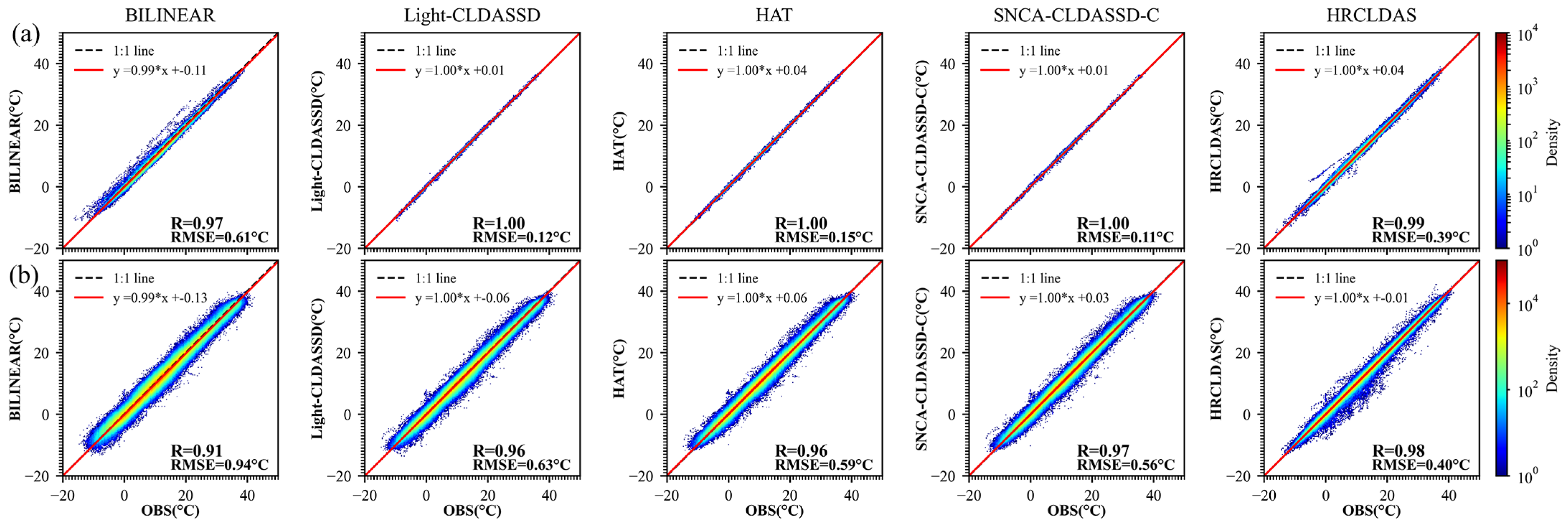
Furthermore, in Figure 4, we present a scatter map illustrating the correlation between observed meteorological station data and interpolated predictions at each time step. The results indicate that, among all methods, SNCA-CLDASSD-C and HRCLDAS exhibit a higher correlation with the observed data. In Figure 4a, all methods are evaluated on non-independent data (CLDAS product data incorporates information from national meteorological stations), but they are temporally independent (the data from 2018 are treated as a separate test set without participation in model training). As a result, all methods show a strong correlation with the national station observations. Among them, the three deep learning models perform even better than HRCLDAS, nearly conforming to the 1:1 line. Particularly, SNCA-CLDASSD-C achieves an average correlation coefficient of 1.0 in 2018, with an RMSE of 0.11 °C, which is 0.31 °C lower than HRCLDAS. In Figure 4b, except for HRCLDAS, which is temporally independent, no method relies on independent data (HRCLDAS product data lack information from regional stations). All methods are temporally and spatially independent (CLDAS product data do not incorporate information from regional stations). Due to the inherent data instability and larger errors in regional meteorological station observations, even after data cleaning, the performance of all methods experiences a certain degree of degradation compared to national station data. The scatter points are more dispersed, reflected from −20 °C to 40 °C. Although HRCLDAS fits the regional stations more closely, it demonstrates a noticeable underestimation within the temperature range of −5 °C to 20 °C. On the other hand, the deep learning model does not exhibit such a phenomenon. Overall, the trend shows that the fit of the deep learning models to station observation data does not fluctuate significantly with temperature changes. Among all deep-learning-based methods, SNCA-CLDASSD-C maintains a respectable average correlation coefficient of no less than 0.97 in 2018, with an RMSE of 0.56 °C, which is 0.07 °C lower than Light-CLDASSD and 0.16 °C higher than HRCLDAS.
3.2. Spatial Distribution
This section focuses on the comprehensive analysis of various downscaling methods’ performance across different underlying surface types (water bodies, islands, plains, and mountainous regions) within the study area. Additionally, a visual comparison is presented to address the occurrence of checkerboard artifacts within the results.
Firstly, we present the evaluation results of various downscaling methods across different underlying surface types in Table 4. Due to the impact of scale effects, the results of bilinear interpolation represent the coarse-scale temperature field of CLDAS, resulting in considerable discrepancies in performance metrics when compared to the finer-scale HRCLDAS. This discrepancy is particularly evident in mountainous regions, where the RMSE of bilinear interpolation is 0.492 °C higher than HRCLDAS when evaluated against both national and regional stations. This reveals the presence of systematic bias. In contrast to bilinear interpolation, Light-CLDASSD, SNCA-CLDASSD-C, and HAT exhibit significant improvements across all aspects. This improvement is attributed to the inclusion of station loss during model training to enhance the reconstruction ability within station areas. Their performance even surpasses that of HRCLDAS at national meteorological stations, though a notable disparity remains when compared to HRCLDAS at the regional stations. Among the three models, SNCA-CLDASSD-C performs the best, followed by HAT and Light-CLDASSD. Indicators from the provided table reveal that our SNCA-CLDASSD-C model demonstrates more evident enhancements in mountainous and plain regions compared to Light-CLDASSD. This improvement is particularly pronounced when validated against the larger dataset of HRCLDAS and regional meteorological observation stations. Specifically, the RMSE decreases by 0.28 °C and 0.17 °C, and the MAE decreases by 0.202 °C and 0.121 °C, respectively. These improvements can be attributed to SCAM’s critical role in capturing spatial texture details from the DEM. Furthermore, the overall comparison of evaluation metrics in Table 4 highlights that SNCA-CLDASSD-C outperforms other models in pixel-level accuracy, spatial structure, and visual similarity. Moreover, in comparison to HRCLDAS, SNCA-CLDASSD-C demonstrates a certain level of advantage and competitiveness.
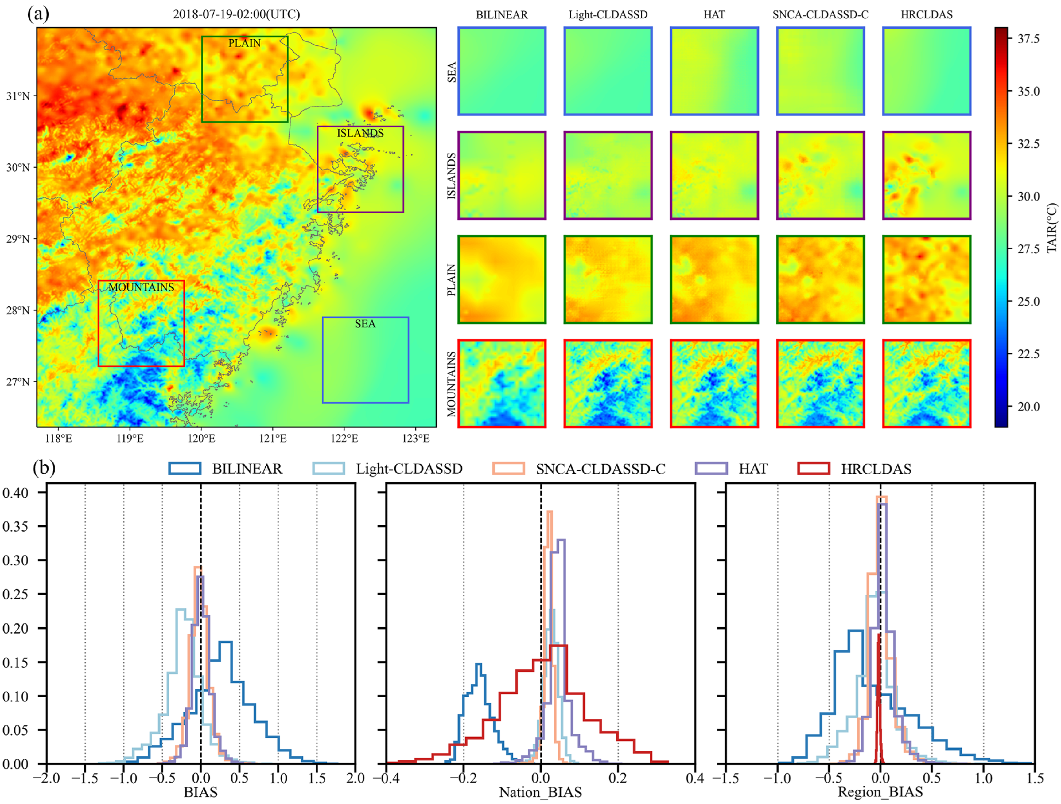
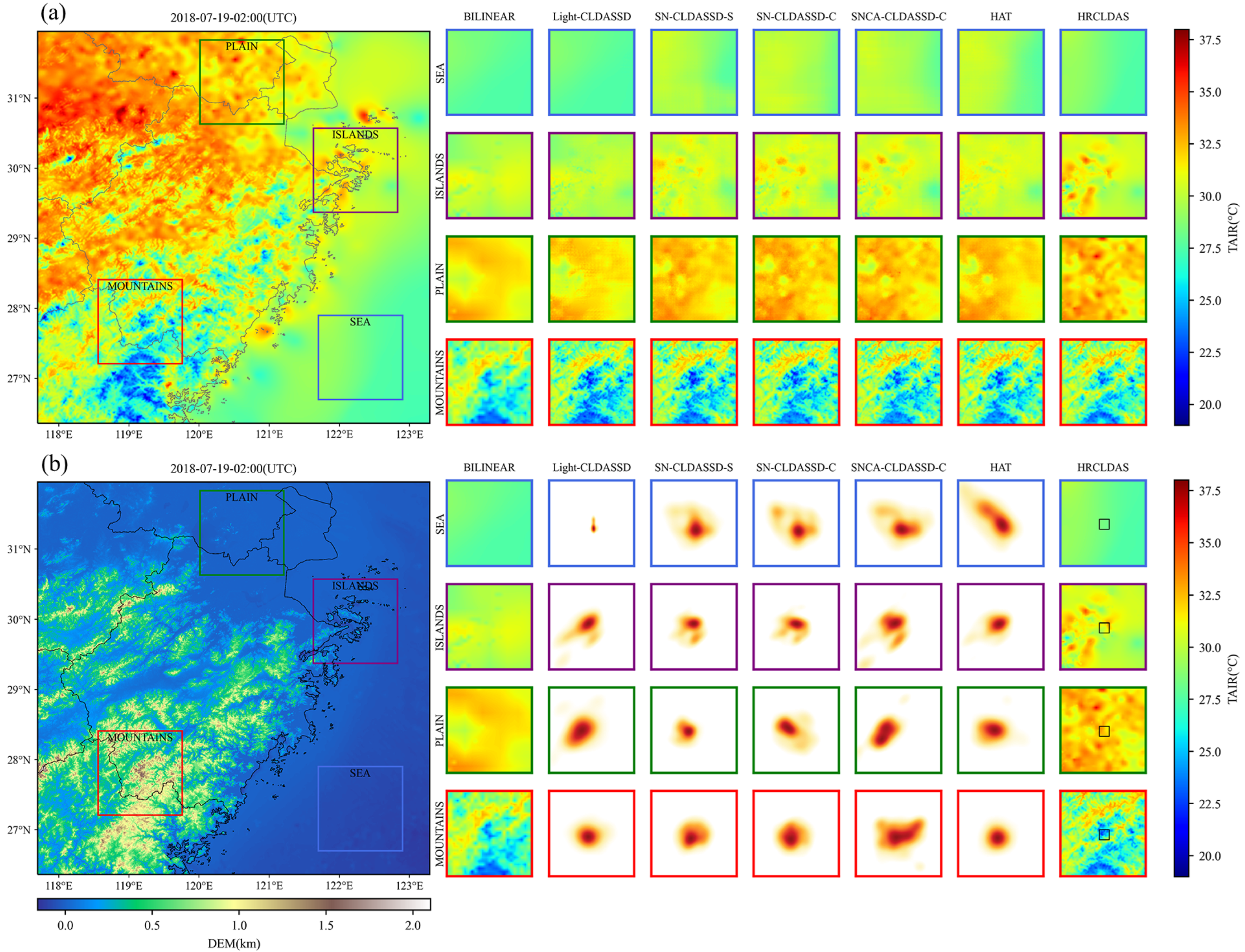
Secondly, as shown in Figure 5a, the HRCLDAS image at 02:00 UTC on 19 July 2018 is displayed on the left-hand side, while the right-hand side presents localized images of various methods for each underlying surface classification. From the visual comparison of these images, it is evident that traditional bilinear interpolation only increases the grid count to form a blurry and coarse representation during downscaling. In contrast, deep learning models, by incorporating DEM information, are capable of better reconstructing spatial details and textures of the temperature field, especially in mountainous, plain, and island areas, bringing the results closer to those of HRCLDAS. Among all methods, only SNCA-CLDASSD-C manages to capture the spatial distribution details between high and low temperatures in the island and plain regions. However, due to the lack of rich texture information from the DEM in oceanic areas, there still exists a significant overestimation phenomenon, along with some degree of underestimation in plain and island regions. Furthermore, we conducted histogram statistics of the bias distribution for all samples in the test set. As depicted in Figure 5b, the control of bias by the bilinear interpolation method is notably weaker than that of other methods. SNCA-CLDASSD-C demonstrates the most stable control of bias, albeit with an overall slight underestimation, approximately around −0.024 °C. Notably, when evaluated against national meteorological station observations, HRCLDAS exhibits a widely dispersed bias distribution, whereas it becomes significantly centered around zero when evaluated against regional meteorological station observations. This could be attributed to the dense incorporation of regional station observations in HRCLDAS, which impacts the sparse national station observations. Conversely, our SNCA-CLDASSD-C model remains unaffected by this phenomenon, highlighting its advantage in this aspect.
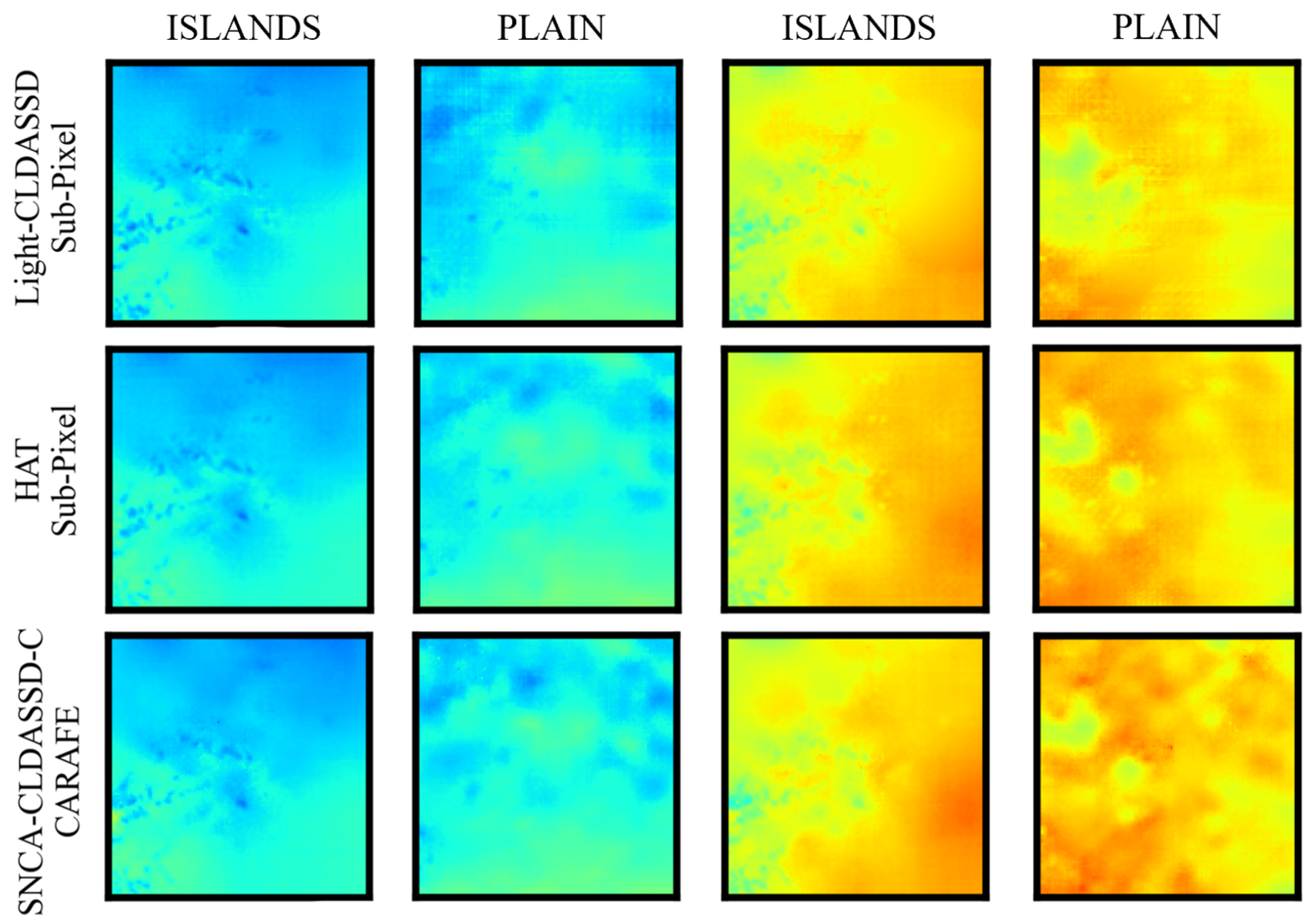
Lastly, in Figure 6, we provide visual zoom-in comparisons in the islands and plain regions between CARAFE and sub-pixel upsampling techniques. According to Table 2, we choose Light-CLDASSD, SNCA-CLDASSD-C, and HAT to show the improvement of our model. Light-CLDASSD and HAT, employing sub-pixel, exhibit varying degrees of checkerboard artifacts and pseudo-shadow phenomena. In contrast, SNCA-CLDASSD-C, utilizing CARAFE, effectively suppresses the occurrence of checkerboard artifacts, which can be seen by comparing the reconstruction results of two upsampling methods in the low-temperature region of column 2 and the high-temperature region of column 4, as well as the sea area in islands region. Compared to the other two methods for reconstructing the fragmented and striped temperature field, the temperature field reconstructed by SNCA-CLDASSD-C exhibits a more comprehensive spatial distribution of high and low temperatures, along with a more continuous texture detail. Furthermore, CARAFE tends to overlook small islands in island regions, as evident from the comparison of the two upsampling methods in columns 1 and 3.
3.3. Temporal Change
In this section, a comprehensive comparative analysis of the results obtained from various downscaling methods is performed, focusing on the temporal variation characteristics.
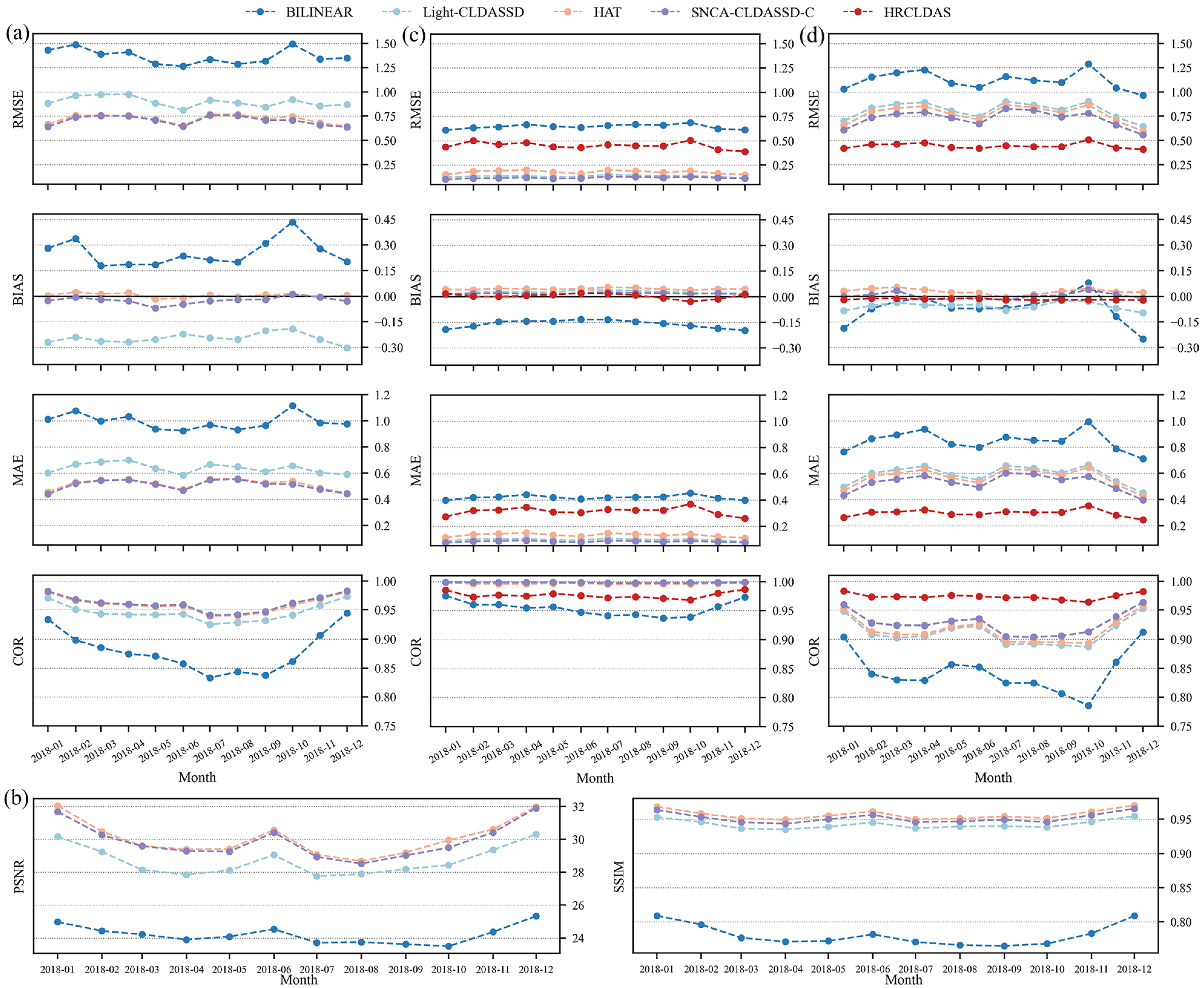
Firstly, in Figure 7a–d, the monthly average temperature RMSE, BIAS, MAE, COR, PSNR, and SSIM for each downscaling method are computed against HRCLDAS, national, and regional meteorological station data as reference values. Overall, all models exhibit a similar trend in the temporal variation of these metrics, with the best performance observed during winter and followed by autumn. Spring and summer seasons show a comparatively poorer performance due to the significant temperature fluctuations caused by the influence of the East Asian monsoon and the warm and humid summer monsoon in the study area. Notably, the deep learning models consistently outperform bilinear interpolation, with SNCA-CLDASS-C and HAT exhibiting a superior performance, especially the bias. Moreover, deep-learning-based methods have better fitting and reconstruction capabilities than HRCLDAS in sparse observations, but there is still a certain gap compared to HRCLDAS in fitting the dense observations. The utilization of the SNBlock, SCAM, and CARAFE in SNCA-CLDASS-C results in a more intricate structural design compared to Light-CLDASSD, incorporating a terrain attention module and improving the upsampling algorithm, leading to a more pronounced disparity. Moreover, our CNN-based model outperforms the state-of-the-art single-image super-resolution SOTA method HAT, which utilizes an improved Swin Transformer for image super-resolution.
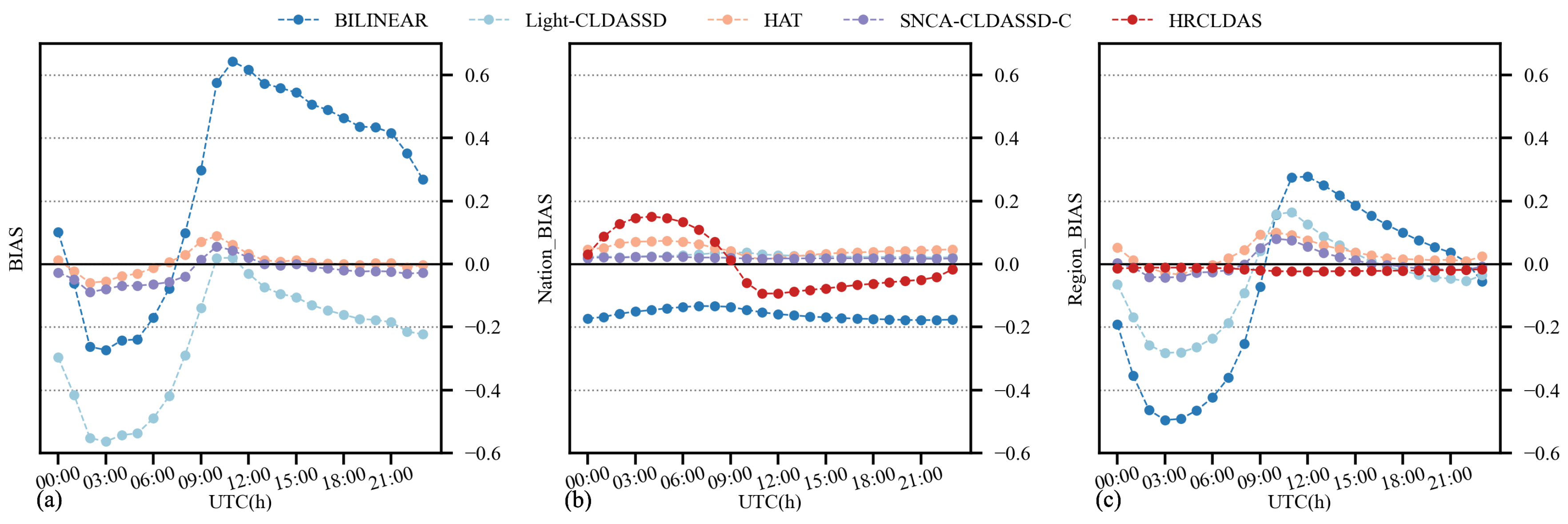
Additionally, Figure 8 presents a comparative analysis of various downscaling methods’ intraday temperature deviation. It can be observed that Light-CLDASSD, compared to bilinear interpolation, shows limited improvement in intraday deviation, particularly at the national meteorological stations. In contrast, SNCA-CLDASS-C and HAT manage to effectively control the intraday deviation, maintaining it at near zero while reducing the magnitude of variation. When evaluated against HRCLDAS and regional stations, the intraday temperature bias of all models is larger during the daytime and smaller during the night-time. In the case of national meteorological stations, the bias is larger during the night-time and smaller during the daytime. However, SNCA-CLDASS-C remarkably flattens the deviation curve, although it exhibits a slight overall overestimation, approximately around 0.019 °C. In conclusion, SNCA-CLDASS-C demonstrates exceptional control over the intraday deviation variation in the results.
3.4. Local Attribution Analysis
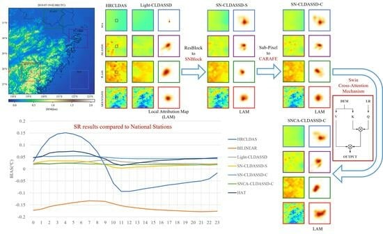
We employed an attribution interpretation method called local attribution mapping (LAM) [42], specifically designed for image super-resolution methods. LAM reveals which input pixels contribute most to a selected region by attributing certain features (using gradient detectors to quantify the presence of edges and textures) to the distribution of locally activated pixels in the output image. As illustrated in Figure 9b, among all models, only the attention of the SNCA-CLDASS-C network with the SCAM is distributed along the direction of DEM texture extension, particularly evident in the complex mountainous region highlighted by the red box. Additionally, we observe that Light-CLDASSD, in comparison to HAT, also attends to a wide range of pixels, yet it still misrepresents textures. Therefore, although Light-CLDASSD employs information from more pixels, it fails to effectively use them for accurate reconstruction and may even compromise the temperature accuracy within the small black box.
4. Discussion
The statistical downscaling approach based on deep learning offers substantial computational advantages over traditional dynamical downscaling. As model resolution increases, it avoids exponential complexity growth and eliminates the need for extensive parameter adjustments, thus saving time and computational resources [43]. Moreover, it offers greater flexibility in local study areas and the design of specific implementation strategies [44].
The SNCA-CLDASSD-C model demonstrates certain advantages over HAT and exhibits a competitive edge compared to HRCLDAS through improvements made to different modules of the Light-CLDASSD network. Given the high correlation between the DEM and temperature, complex terrain variations inevitably impact the spatiotemporal temperature distribution. Although the selected study area has modest terrain fluctuations, its diverse terrain types and location in eastern mainland China, affected by monsoon variations and typhoons, result in substantial temperature fluctuations during the rainy and hot summer [45,46]. As elaborated in Section 3 of this paper, our improved SNCA-CLDASSD-C model not only learns more complex mapping relationships but also addresses the limited spatial detail reconstruction ability of Light-CLDASSD in plain areas. The incorporation of DEM-based cross-attention contributes to an enhanced focus on and understanding of DEM-derived information for reconstructing temperature trends and details in complex mountainous terrain. Our model exhibits superior stability and control over bias, particularly concerning intraday hourly deviation variations. In addition, SNCA-CLDASSD-C only takes about 45 ms to infer 560 × 560 data for one time, which is more than 100 times faster than traditional dynamic downscaling methods.
While SNCA-CLDASSD-C demonstrates significant strengths, some challenges persist when compared to HRCLDAS. Fitting regional meteorological station data and reconstructing sea near-surface temperatures remain areas of improvement. The distribution density of regional stations in the study area leads to extremely high and low temperatures, as well as highly detailed spatial textures, under the assumption of unbiased estimation, which may not be perfectly reconstructed by our model. Nevertheless, HRCLDAS is not the true value, and the quality of observations from regional stations is also unstable, making this discrepancy not a sufficient criterion to measure our model’s performance. Additionally, the absence of DEM values in sea areas hinders spatial detail, providing limited spatial detail information, and the primary driving factor for sea near-surface temperature variations is not the terrain. Therefore, supplementary auxiliary data like air pressure and wind speed can be considered in such cases.
Furthermore, there is potential to further enhance the utilization of auxiliary data. The integration of cross-attention mechanisms for utilizing data like land use information in tasks related to various meteorological variables holds promise. Additionally, the modular design of the study creates opportunities for other deep learning downscaling networks to benefit from the fusion of terrain and feature information modules, thereby improving the overall model performance.
5. Conclusions
This paper introduces the SNCA-CLDASSD network model, utilizing deep learning for spatially downscaling CLDAS temperature data from 0.05° to 0.01°. The SNCA-CLDASSD model incorporates the SNBlock, SCAM, and CARAFE, and employs ablation experiments to validate its performance enhancement over Light-CLDASSD. Data from 2016, 2017, 2019, and 2020 were used, with 90% for training, 10% for validation, and 2018 as an independent test set. During training, the DEM was introduced as auxiliary data, and a loss function incorporating station observation data was employed for soft constraint. Through the evaluation and analysis of the results for various methods, the following conclusions are obtained:
- The SNCA-CLDASSD-C model, incorporating the SNBlock, SCAM, and CARAFE, exhibits the best performance among all variations. Compared to Light-CLDASSD, it significantly improves the spatial downscaling accuracy.
- The SNCA-CLDASSD-C model shows the most improvement in mountainous areas compared to Light-CLDASSD, followed by plain areas. Additionally, CARAFE effectively reduces checkerboard patterns compared to sub-pixel. Furthermore, the CARAFE upsampling operator effectively suppresses the checkerboard artifacts compared to sub-pixel.
- Our model performs best in winter, and then in autumn, but has a relatively lower performance in spring and summer. It also has the least bias, especially in hourly temperature.
- Through local attribution analysis (LAM) of various downscaling methods, it is evident that the SCAM effectively utilizes high-resolution auxiliary data such as the DEM to enhance model performance. The SCAM adeptly extracts feature information from these auxiliary data sources, allowing for the reconstruction of more detailed temperature field textures.
Author Contributions
Conceptualization, Z.S. and C.S.; methodology, Z.S. and R.T.; software, Z.S.; validation, Z.S. and L.G.; formal analysis, Z.S.; investigation, Z.S.; resources, C.S.; data curation, Z.S.; writing—original draft preparation, Z.S.; writing—review and editing, Z.S. and L.G.; visualization, Z.S.; supervision, L.G. and C.S.; project administration, C.S. and R.S.; funding acquisition, C.S. All authors have read and agreed to the published version of the manuscript.
Funding
This research was funded by advanced research on civil space technology during the 14th Five-Year Plan, National Meteorological Information Center of China Meteorological (NMICJY202305), GHFUND C (202302035765) and the National Nature Science Foundation of China (91437105, 92037000 and 42205153).
Data Availability Statement
Acknowledgments
We thank the National Meteorological Information Center of China Meteorological Administration for data support.
Conflicts of Interest
The authors declare no conflict of interest.
References
- Han, S.; Shi, C.; Xu, B.; Sun, S.; Zhang, T.; Jiang, L.; Liang, X. Development and evaluation of hourly and kilometer resolution retrospective and real-time surface meteorological blended forcing dataset (SMBFD) in China. J. Meteorol. Res. 2019, 33, 1168–1181. [Google Scholar] [CrossRef]
- Huang, X.; Rhoades, A.M.; Ullrich, P.A.; Zarzycki, C.M. An evaluation of the variable-resolution CESM for modeling California’s climate. J. Adv. Model. Earth Syst. 2016, 8, 345–369. [Google Scholar] [CrossRef]
- Chen, L.; Liang, X.Z.; DeWitt, D.; Samel, A.N.; Wang, J.X. Simulation of seasonal US precipitation and temperature by the nested CWRF-ECHAM system. Clim. Dyn. 2016, 46, 879–896. [Google Scholar] [CrossRef]
- Griggs, D.J.; Noguer, M. Climate change 2001: The scientific basis. Contribution of working group I to the third assessment report of the intergovernmental panel on climate change. Weather 2002, 57, 267–269. [Google Scholar] [CrossRef]
- Hertig, E.; Jacobeit, J. Assessments of Mediterranean precipitation changes for the 21st century using statistical downscaling techniques. Int. J. Climatol. J. R. Meteorol. Soc. 2008, 28, 1025–1045. [Google Scholar] [CrossRef]
- Sun, X.; Wang, J.; Zhang, L.; Ji, C.; Zhang, W.; Li, W. Spatial downscaling model combined with the Geographically Weighted Regression and multifractal models for monthly GPM/IMERG precipitation in Hubei Province, China. Atmosphere 2022, 13, 476. [Google Scholar] [CrossRef]
- Stehlík, J.; Bárdossy, A. Multivariate stochastic downscaling model for generating daily precipitation series based on atmospheric circulation. J. Hydrol. 2002, 256, 120–141. [Google Scholar] [CrossRef]
- Kwon, M.; Kwon, H.H.; Han, D. A spatial downscaling of soil moisture from rainfall, temperature, and AMSR2 using a Gaussian-mixture nonstationary hidden Markov model. J. Hydrol. 2018, 564, 1194–1207. [Google Scholar] [CrossRef]
- Ailliot, P.; Allard, D.; Monbet, V.; Naveau, P. Stochastic weather generators: An overview of weather type models. J. De La Société Française De Stat. 2015, 156, 101–113. [Google Scholar]
- Semenov, M.A. Simulation of extreme weather events by a stochastic weather generator. Clim. Res. 2008, 35, 203–212. [Google Scholar] [CrossRef]
- Choi, H.; Lee, J.; Yang, J. N-gram in swin transformers for efficient lightweight image super-resolution. In Proceedings of the IEEE/CVF Conference on Computer Vision and Pattern Recognition, Vancouver, BC, Canada, 17–24 June 2023; pp. 2071–2081. [Google Scholar]
- Wang, P.; Bayram, B.; Sertel, E. A comprehensive review on deep learning based remote sensing image super-resolution methods. Earth-Sci. Rev. 2022, 232, 104110. [Google Scholar] [CrossRef]
- Chan, K.C.; Zhou, S.; Xu, X.; Loy, C.C. Basicvsr++: Improving video super-resolution with enhanced propagation and alignment. In Proceedings of the IEEE/CVF Conference on Computer Vision and Pattern Recognition, New Orleans, LA, USA, 18–24 June 2022; pp. 5972–5981. [Google Scholar]
- Ranade, R.; Liang, Y.; Wang, S.; Bai, D.; Lee, J. 3D Texture Super Resolution via the Rendering Loss. In Proceedings of the ICASSP 2022-2022 IEEE International Conference on Acoustics, Speech and Signal Processing (ICASSP), Virtual, 7–13 May 2022; IEEE: Piscataway, NJ, USA, 2022; pp. 1556–1560. [Google Scholar]
- Wang, F.; Tian, D.; Lowe, L.; Kalin, L.; Lehrter, J. Deep learning for daily precipitation and temperature downscaling. Water Resour. Res. 2021, 57, e2020WR029308. [Google Scholar] [CrossRef]
- Harris, L.; McRae, A.T.; Chantry, M.; Dueben, P.D.; Palmer, T.N. A generative deep learning approach to stochastic downscaling of precipitation forecasts. J. Adv. Model. Earth Syst. 2022, 14, e2022MS003120. [Google Scholar] [CrossRef]
- Leinonen, J.; Nerini, D.; Berne, A. Stochastic super-resolution for downscaling time-evolving atmospheric fields with a generative adversarial network. IEEE Trans. Geosci. Remote Sens. 2020, 59, 7211–7223. [Google Scholar] [CrossRef]
- Vandal, T.; Kodra, E.; Ganguly, S.; Michaelis, A.; Nemani, R.; Ganguly, A.R. Deepsd: Generating high resolution climate change projections through single image super-resolution. In Proceedings of the 23rd ACM SIGKDD International Conference on Knowledge Discovery and Data Mining, Halifax, NS, Canada, 13–17 August 2017; pp. 1663–1672. [Google Scholar]
- Mao, Z. Spatial Downscaling of Meteorological Data Based on Deep Learning Image Super-Resolution. Master’s Thesis, Wuhan University, Wuhan, China, 2019. [Google Scholar]
- Singh, A.; White, B.; Albert, A.; Kashinath, K. Downscaling numerical weather models with GANs. In Proceedings of the 100th American Meteorological Society Annual Meeting, Boston, MA, USA, 12–16 January 2020. [Google Scholar]
- Höhlein, K.; Kern, M.; Hewson, T.; Westermann, R. A comparative study of convolutional neural network models for wind field downscaling. Meteorol. Appl. 2020, 27, e1961. [Google Scholar] [CrossRef]
- Gerges, F.; Boufadel, M.C.; Bou-Zeid, E.; Nassif, H.; Wang, J.T. A novel deep learning approach to the statistical downscaling of temperatures for monitoring climate change. In Proceedings of the 2022 6th International Conference on Machine Learning and Soft Computing, Haikou, China, 15–17 January 2022; pp. 1–7. [Google Scholar]
- Tie, R.; Shi, C.; Wan, G.; Hu, X.; Kang, L.; Ge, L. CLDASSD: Reconstructing fine textures of the temperature field using super-resolution technology. Adv. Atmos. Sci. 2022, 39, 117–130. [Google Scholar] [CrossRef]
- Tie, R.; Shi, C.; Wan, G.; Kang, L.; Ge, L. To Accurately and Lightly Downscale the Temperature Field by Deep Learning. J. Atmos. Ocean. Technol. 2022, 39, 479–490. [Google Scholar] [CrossRef]
- Liu, Z.; Lin, Y.; Cao, Y.; Hu, H.; Wei, Y.; Zhang, Z.; Lin, S.; Guo, B. Swin transformer: Hierarchical vision transformer using shifted windows. In Proceedings of the IEEE/CVF International Conference on Computer Vision, Montreal, BC, Canada, 11–17 October 2021; pp. 10012–10022. [Google Scholar]
- Chen, C.F.R.; Fan, Q.; Panda, R. Crossvit: Cross-attention multi-scale vision transformer for image classification. In Proceedings of the IEEE/CVF International Conference on Computer Vision, Montreal, BC, Canada, 11–17 October 2021; pp. 357–366. [Google Scholar]
- Han, S.; Liu, B.; Shi, C.; Liu, Y.; Qiu, M.; Sun, S. Evaluation of CLDAS and GLDAS datasets for Near-surface Air Temperature over major land areas of China. Sustainability 2020, 12, 4311. [Google Scholar] [CrossRef]
- Reuter, H.I.; Nelson, A.; Jarvis, A. An evaluation of void-filling interpolation methods for SRTM data. Int. J. Geogr. Inf. Sci. 2007, 21, 983–1008. [Google Scholar] [CrossRef]
- QX/T 118-2020; Meteorological Observation Data Quality Control. Chinese Industry Standard: Beijing, China, 2020.
- He, K.; Zhang, X.; Ren, S.; Sun, J. Deep residual learning for image recognition. In Proceedings of the IEEE Conference on Computer Vision and Pattern Recognition, Las Vegas, NV, USA, 26 June–1 July 2016; pp. 770–778. [Google Scholar]
- Zhang, X.; Zhou, X.; Lin, M.; Sun, J. Shufflenet: An extremely efficient convolutional neural network for mobile devices. In Proceedings of the IEEE Conference on Computer Vision and Pattern Recognition, Salt Lake City, UT, USA, 18–23 June 2018; pp. 6848–6856. [Google Scholar]
- Chen, L.; Chu, X.; Zhang, X.; Sun, J. Simple baselines for image restoration. In Proceedings of the European Conference on Computer Vision, Tel Aviv, Israel, 23–27 October 2022; Springer: Berlin/Heidelberg, Germany, 2022; pp. 17–33. [Google Scholar]
- Hu, J.; Shen, L.; Sun, G. Squeeze-and-excitation networks. In Proceedings of the IEEE Conference on Computer Vision and Pattern Recognition, Salt Lake City, UT, USA, 18–23 June 2018; pp. 7132–7141. [Google Scholar]
- Howard, A.; Sandler, M.; Chu, G.; Chen, L.C.; Chen, B.; Tan, M.; Wang, W.; Zhu, Y.; Pang, R.; Vasudevan, V.; et al. Searching for mobilenetv3. In Proceedings of the IEEE/CVF International Conference on Computer Vision, Seoul, Republic of Korea, 27 October–2 November 2019; pp. 1314–1324. [Google Scholar]
- Vaswani, A.; Shazeer, N.; Parmar, N.; Uszkoreit, J.; Jones, L.; Gomez, A.N.; Kaiser, Ł.; Polosukhin, I. Attention is all you need. Adv. Neural Inf. Process. Syst. 2017, 30, 6000–6010. [Google Scholar]
- Shi, W.; Caballero, J.; Huszár, F.; Totz, J.; Aitken, A.P.; Bishop, R.; Rueckert, D.; Wang, Z. Real-time single image and video super-resolution using an efficient sub-pixel convolutional neural network. In Proceedings of the IEEE Conference on Computer Vision and Pattern Recognition, Las Vegas, NV, USA, 27 June 2016; pp. 1874–1883. [Google Scholar]
- Odena, A.; Dumoulin, V.; Olah, C. Deconvolution and checkerboard artifacts. Distill 2016, 1, e3. [Google Scholar] [CrossRef]
- Wang, J.; Chen, K.; Xu, R.; Liu, Z.; Loy, C.C.; Lin, D. Carafe: Content-aware reassembly of features. In Proceedings of the IEEE/CVF International Conference on Computer Vision, Seoul, Republic of Korea, 27 October–2 November 2019; pp. 3007–3016. [Google Scholar]
- Lai, W.S.; Huang, J.B.; Ahuja, N.; Yang, M.H. Fast and accurate image super-resolution with deep laplacian pyramid networks. IEEE Trans. Pattern Anal. Mach. Intell. 2018, 41, 2599–2613. [Google Scholar] [CrossRef]
- Chen, X.; Wang, X.; Zhou, J.; Qiao, Y.; Dong, C. Activating more pixels in image super-resolution transformer. In Proceedings of the IEEE/CVF Conference on Computer Vision and Pattern Recognition, Seattle, WA, USA, 14–19 June 2023; pp. 22367–22377. [Google Scholar]
- Liang, J.; Cao, J.; Sun, G.; Zhang, K.; Van Gool, L.; Timofte, R. Swinir: Image restoration using swin transformer. In Proceedings of the IEEE/CVF International Conference on Computer Vision, Montreal, BC, Canada, 11–17 October 2021; pp. 1833–1844. [Google Scholar]
- Gu, J.; Dong, C. Interpreting super-resolution networks with local attribution maps. In Proceedings of the IEEE/CVF Conference on Computer Vision and Pattern Recognition, Nashville, TN, USA, 20–25 June 2021; pp. 9199–9208. [Google Scholar]
- Maraun, D.; Wetterhall, F.; Ireson, A.; Chandler, R.; Kendon, E.; Widmann, M.; Brienen, S.; Rust, H.; Sauter, T.; Themeßl, M.; et al. Precipitation downscaling under climate change: Recent developments to bridge the gap between dynamical models and the end user. Rev. Geophys. 2010, 48. [Google Scholar] [CrossRef]
- Wilby, R.L.; Charles, S.P.; Zorita, E.; Timbal, B.; Whetton, P.; Mearns, L.O. Guidelines for Use Of Climate Scenarios Developed From Statistical Downscaling Methods. Supporting material of the Intergovernmental Panel on Climate Change, available from the DDC of IPCC TGCIA. 2004. Available online: https://www.ipcc-data.org/guidelines/dgm_no2_v1_09_2004.pdf (accessed on 1 August 2004).
- Hao, M.; Changjie, L.; Qifeng, Q.; Zheyong, X.; Jingjing, X.; Ming, Y.; Dawei, G. Analysis on Climatic Characteristics of Extreme High-temperature in Zhejiang Province in May 2018 and Associated Large-scale Circulation. J. Arid Meteorol. 2020, 38, 909. [Google Scholar]
- Jianjiang, W.; Hao, M.; Liping, Y.; Liqing, G.; Chen, W. Analysis of Atmospheric Circulation Characteristics Associated with Autumn Drought over Zhejiang Province in 2019. J. Arid Meteorol. 2021, 39, 1. [Google Scholar]
- Chen, F.; Manning, K.W.; LeMone, M.A.; Trier, S.B.; Alfieri, J.G.; Roberts, R.; Tewari, M.; Niyogi, D.; Horst, T.W.; Oncley, S.P.; et al. Description and evaluation of the characteristics of the NCAR high-resolution land data assimilation system. J. Appl. Meteorol. Climatol. 2007, 46, 694–713. [Google Scholar] [CrossRef]
Figure 1.
The left image depicts the spatial distribution of national meteorological stations (red star markers) and regional stations (green triangle markers) within the study area. The right image illustrates the spatial distribution of DEM across the study area.
Figure 1.
The left image depicts the spatial distribution of national meteorological stations (red star markers) and regional stations (green triangle markers) within the study area. The right image illustrates the spatial distribution of DEM across the study area.

Figure 2.
Column 1 depicts the histogram of mean absolute error (MAE) and correlation coefficient (COR) for regional station data. Column 2 displays the violin plot of MAE and COR for regional station data before data cleaning. Column 3 showcases the violin plot of MAE and COR for regional station data after data cleaning.

Figure 3.
(a) Overview of the proposed SNCA-CLDASSD model structure. (b) Overview of Shuffle–nonlinear-activation-free block (SNBlock). (c) Overview of simplified channel attention. (d) Overview of simple gate. (e) Overview of Swin cross-attention (SCAM). (f) Overview of cross-windows attention.
Figure 3.
(a) Overview of the proposed SNCA-CLDASSD model structure. (b) Overview of Shuffle–nonlinear-activation-free block (SNBlock). (c) Overview of simplified channel attention. (d) Overview of simple gate. (e) Overview of Swin cross-attention (SCAM). (f) Overview of cross-windows attention.

Figure 4.
(a) Scatter density map between observed values from national meteorological stations and interpolated predictions at station locations; (b) scatter density map between observed values from regional stations and interpolated predictions at station locations. (Different from Table 3, here, the data are after data cleaning and are not of all time steps in 2018.)

Figure 5.
(a) Visual comparison of the results for various methods at 02:00 UTC on 19 July 2018. The large left image represents the HRCLDAS image; (b) spatial bias histograms for all samples in the test set. Column 1 is evaluated against HRCLDAS as the reference value, column 2 is evaluated against national meteorological station observations as the reference value, and column 3 is evaluated against regional meteorological station observations as the reference value.

Figure 6.
Visual comparison of the results using CARAFE and sub-pixel upsampling method. Column 1, 3 are in the islands region, and column 2, 4 are in the plain region.
Figure 6.
Visual comparison of the results using CARAFE and sub-pixel upsampling method. Column 1, 3 are in the islands region, and column 2, 4 are in the plain region.

Figure 7.
Monthly inter seasonal trend lines of RMSE, BIAS, MAE, PSNR, and SSIM. (a) The RMSE, BIAS, MAE, and COR with HRCLDAS as the ground truth for the results of various methods; (b) the PSNR and SSIM with HRCLDAS as the ground truth for the results of various methods; (c) the RMSE, BIAS, MAE, and COR with national stations as the ground truth for the results of various methods; (d) the RMSE, BIAS, MAE, and COR with regional stations as the ground truth for the results of various methods. (Here, the data are of all time steps.)

Figure 8.
Intraday trend lines of BIAS. (a) The BIAS with HRCLDAS as the ground truth for the results of various methods; (b) the BIAS with national stations as the ground truth for the results of various methods; (c) the BIAS with regional stations as the ground truth for the results of various methods. (Here, the data are of all time steps.)

Figure 9.
(a) Visual comparison of the results for various methods at 02:00 UTC on 19 July 2018. The large left image represents the HRCLDAS image; (b) local attribution mapping (LAM) of the results for various methods at 02:00 UTC on 19 July 2018. LAM reflects the importance of each pixel in the input LR image when reconstructing the patch marked by the small black box. The large left image represents the DEM image.


Table 1.
Descriptions of all types of datasets (all datasets are projected by equal latitude–longitude projection).
Table 1.
Descriptions of all types of datasets (all datasets are projected by equal latitude–longitude projection).
| Dataset | Spatial Resolution | Range | Source |
|---|---|---|---|
| CLDAS | 0.05° | 2016.01–2020.12 (hourly) | NMIC |
| HRCLDAS | 0.01° | 2016.01–2020.12 (hourly) | NMIC |
| SRTM(DEM) | 0.01° | - | NASA |
| Station Observation | - | 2016.01–2020.12 (hourly) | NMIC |
Table 2.
Table of ablation study.
| Model | Feature Extraction Block | SCAM | Upsampling Module |
|---|---|---|---|
| Light-CLDASSD | ResBlock | - | Sub-Pixel |
| SN-CLDASSD-S | SNBlock | - | Sub-Pixel |
| SN-CLDASSD-C | SNBlock | - | CARAFE |
| SNCA-CLDASSD-C | SNBlock | √ | CARAFE |
Table 3.
Comprehensive evaluation metrics table of downscaling results by various methods; evaluation metrics are assessed using HRCLDAS, national meteorological stations, and regional stations as reference values, with the optimal metrics indicated in bold. (Here, the data are of all time steps.)
Table 3.
Comprehensive evaluation metrics table of downscaling results by various methods; evaluation metrics are assessed using HRCLDAS, national meteorological stations, and regional stations as reference values, with the optimal metrics indicated in bold. (Here, the data are of all time steps.)
| Methods | HRCLDAS/Nation Stations/Region Stations | PSNR | SSIM | ||
|---|---|---|---|---|---|
| RMSE | MAE | COR | |||
| BILINEAR | 1.365/0.646/1.118 | 0.993/0.419/0.845 | 0.879/0.954/0.844 | 24.206 | 0.781 |
| Light-CLDASSD | 0.898/0.134/0.810 | 0.638/0.096/0.589 | 0.946/0.998/0.912 | 28.707 | 0.943 |
| SN-CLDASSD-S | 0.713/0.163/0.771 | 0.514/0.119/0.565 | 0.960/0.997/0.917 | 29.981 | 0.953 |
| SN-CLDASSD-C | 0.711/0.131/0.727 | 0.514/0.093/0.531 | 0.961/0.998/0.927 | 30.027 | 0.954 |
| SNCA-CLDASSD-C | 0.706/0.118/0.724 | 0.507/0.082/0.527 | 0.961/0.998/0.928 | 30.083 | 0.957 |
| HAT | 0.720/0.178/0.774 | 0.515/0.131/0.566 | 0.959/0.996/0.916 | 29.899 | 0.952 |
| HRCLDAS | - /0.450/0.443 | - /0.313/0.296 | - /0.976/0.974 | - | - |
Table 4.
Evaluation metrics of different downscaling methods on four distinct underlying surface types: water bodies, islands, plains, and mountainous regions. The division between plains and mountainous regions is based on a terrain undulation threshold of 30 m, while water bodies and islands are determined using the 2018 CNLUCC land use data. Evaluation metrics are assessed using HRCLDAS, national meteorological stations, and regional stations as reference values, with the optimal metrics highlighted in bold. (Here, the data are of all time steps.)
| Methods | Topography | HRCLDAS/Nation Stations/Region Stations | ||
|---|---|---|---|---|
| RMSE | MAE | COR | ||
| BILINEAR | Water | 1.113/0.336/1.009 | 0.849/0.250/0.769 | 0.852/0.981/0.812 |
| Island | 0.839/0.236/0.967 | 0.630/0.193/0.761 | 0.772/0.974/0.715 | |
| Plain | 0.994/0.521/1.013 | 0.704/0.370/0.760 | 0.838/0.961/0.832 | |
| Mountains | 1.732/1.162/1.325 | 1.346/0.816/1.046 | 0.754/0.974/0.812 | |
| Light-CLDASSD | Water | 0.741/0.093/0.800 | 0.539/0.071/0.585 | 0.912/0.999/0.883 |
| Island | 0.668/0.073/0.744 | 0.503/0.059/0.560 | 0.867/0.998/0.844 | |
| Plain | 0.775/0.125/0.741 | 0.551/0.092/0.540 | 0.906/0.997/0.904 | |
| Mountains | 1.088/0.187/0.924 | 0.806/0.136/0.688 | 0.908/0.998/0.892 | |
| SNCA-CLDASSD-C | Water | 0.638/0.092/0.697 | 0.467/0.072/0.511 | 0.929/0.998/0.907 |
| Island | 0.527/0.081/0.640 | 0.394/0.066/0.485 | 0.903/0.997/0.878 | |
| Plain | 0.605/0.104/0.670 | 0.430/0.077/0.488 | 0.934/0.998/0.920 | |
| Mountains | 0.808/0.175/0.823 | 0.604/0.117/0.613 | 0.938/0.998/0.911 | |
| HAT | Water | 0.648/0.154/0.749 | 0.467/0.117/0.554 | 0.923/0.996/0.892 |
| Island | 0.542/0.147/0.702 | 0.406/0.119/0.537 | 0.896/0.991/0.852 | |
| Plain | 0.623/0.174/0.713 | 0.443/0.130/0.523 | 0.930/0.995/0.908 | |
| Mountains | 0.825/0.200/0.881 | 0.617/0.148/0.658 | 0.934/0.998/0.895 | |
| HRCLDAS | Water | - /0.424/0.379 | - /0.324/0.240 | - /0.965/0.974 |
| Island | - /0.407/0.333 | - /0.314/0.246 | - /0.918/0.969 | |
| Plain | - /0.387/0.403 | - /0.269/0.265 | - /0.975/0.972 | |
| Mountains | - /0.670/0.531 | - /0.519/0.379 | - /0.974/0.963 | |
Disclaimer/Publisher’s Note: The statements, opinions and data contained in all publications are solely those of the individual author(s) and contributor(s) and not of MDPI and/or the editor(s). MDPI and/or the editor(s) disclaim responsibility for any injury to people or property resulting from any ideas, methods, instructions or products referred to in the content. |
© 2023 by the authors. Licensee MDPI, Basel, Switzerland. This article is an open access article distributed under the terms and conditions of the Creative Commons Attribution (CC BY) license (https://creativecommons.org/licenses/by/4.0/).
Share and Cite
MDPI and ACS Style
Shen, Z.; Shi, C.; Shen, R.; Tie, R.; Ge, L. Spatial Downscaling of Near-Surface Air Temperature Based on Deep Learning Cross-Attention Mechanism. Remote Sens. 2023, 15, 5084. https://doi.org/10.3390/rs15215084
AMA Style
Shen Z, Shi C, Shen R, Tie R, Ge L. Spatial Downscaling of Near-Surface Air Temperature Based on Deep Learning Cross-Attention Mechanism. Remote Sensing. 2023; 15(21):5084. https://doi.org/10.3390/rs15215084
Chicago/Turabian StyleShen, Zhanfei, Chunxiang Shi, Runping Shen, Ruian Tie, and Lingling Ge. 2023. "Spatial Downscaling of Near-Surface Air Temperature Based on Deep Learning Cross-Attention Mechanism" Remote Sensing 15, no. 21: 5084. https://doi.org/10.3390/rs15215084
Note that from the first issue of 2016, this journal uses article numbers instead of page numbers. See further details here.