
Two-Step Correction Based on In-Situ Sound Speed Measurements for USBL Precise Real-Time Positioning

1
State Key Laboratory of Geo-Information Engineering, Xi’an 710054, China
2
Chinese Academy of Surveying and Mapping, Beijing 100036, China
3
China Geological Survey, Qingdao Institute of Marine Geology, Qingdao 266237, China
4
College of Oceanography and Space Informatics, China University of Petroleum, Qingdao 266580, China
*
Author to whom correspondence should be addressed.
Remote Sens. 2023, 15(20), 5046; https://doi.org/10.3390/rs15205046
Submission received: 5 September 2023
/
Revised: 13 October 2023
/
Accepted: 18 October 2023
/
Published: 20 October 2023
(This article belongs to the Special Issue Navigation, Localization and Applications for Unmanned Marine Vehicles and Systems)
Abstract
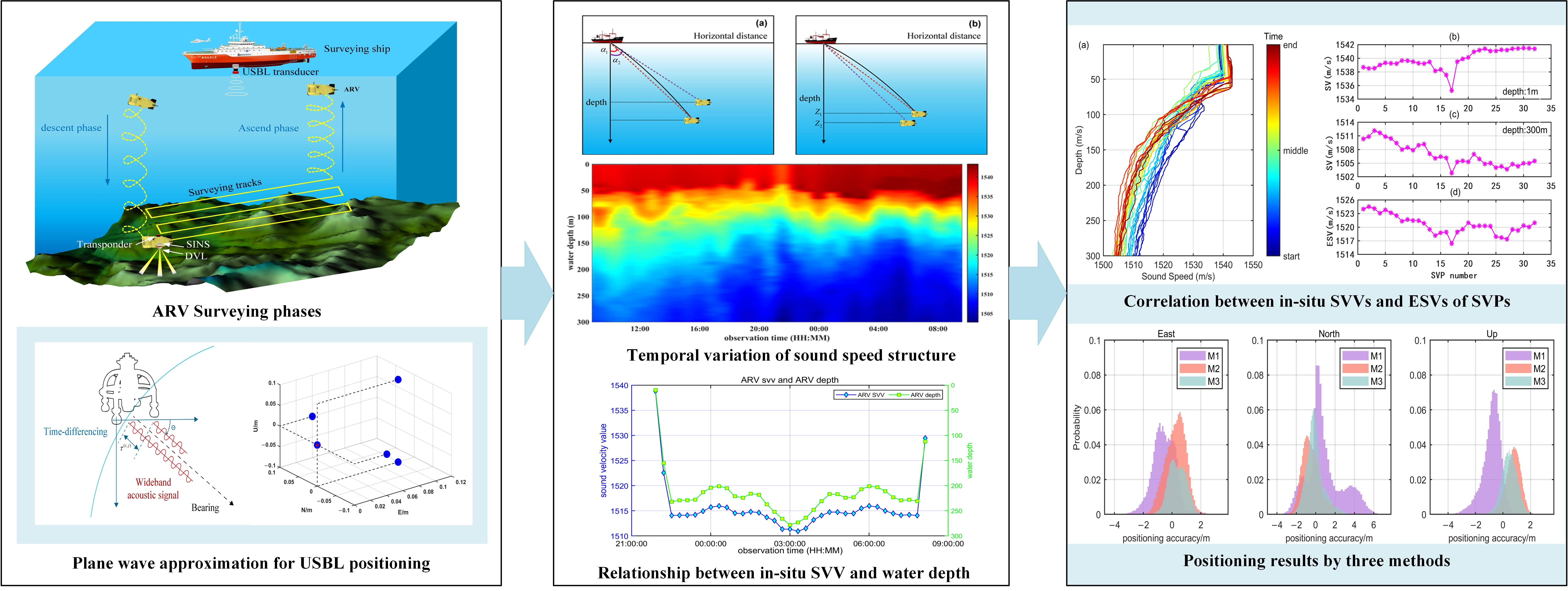
:The ultra-short baseline (USBL) positioning system has been widely used for autonomous and remotely operated vehicle (ARV) positioning in marine resource surveying and ocean engineering fields due to its flexible installation and portable operation. Errors related to the sound speed are a critical factor limiting the positioning performance. The conventional strategy adopts a fixed sound velocity profile (SVP) to correct the spatial variation, especially in the vertical direction. However, SVP is actually time-varying, and ignoring this kind of variation will lead to a worse estimation of ARVs’coordinates. In this contribution, we propose a two-step sound speed correction method, where, firstly, the deviation due to the acoustic ray bending effect is corrected by the depth-based ray-tracing policy with the fixed SVP. Then, the temporal variation of SVP is considered, and the fixed SVP is adaptively adjusted according to the in situ sound velocity (SV) measurements provided by the conductivity–temperature–depth (CTD) sensor equipped at the ARV. The proposed method is verified by semi-physical simulation and sea-trail dataset in the South China Sea. When compared to the fixed-SVP method, average positioning accuracy with the resilient SVP be improved by 8%, 21%, and 26% in the east, north, and up directions, respectively. The results demonstrate that the proposed method can efficiently improve the adaptability of sound speed observations and deliver better performance in USBL real-time positioning.

1. Introduction
Underwater positioning technology plays a vital role in autonomous and remotely operated vehicles (ARVs) to smoothly cruise, avoid obstacles, and carry out underwater operations. Due to the strong penetration of acoustic signals in the ocean environment, Underwater Acoustic-Dominated Positioning Systems (UAPS) show absolute superiority in the ocean [1,2,3,4]. According to the baseline length of the acoustic array, UAPS is broadly categorized into Long Baselines (LBL), Short Baselines (SBL), Ultra-Short Baselines (USBL), and Mixed-Baseline systems [5,6,7]. The USBL positioning system has the advantages of small size, flexible installation, and portable operation, which makes it widely applicable for ARVs’ acoustic positioning for shallow water environments and for providing aided integrated navigation for deep water missions [8,9]. The USBL positioning system mainly includes a meter-level-sized acoustic array composed of one transmitter and multiple receivers, mounted at the bottom of the support ship and the responder unit installed on the ARV. The transmitter sends the inquiry signals to the responder, and the receivers receive the feedback interrogating signals from the responder; hence, the time-of-arrival (TOA) or phase-of-arrival (POA) of traveling acoustic signals for each receiver in one ask–answer cycle has been recorded. Generally, the time difference of arrival (TDOA) or phase difference of arrival (PDOA) between array elements can be calculated to determine the relative positions of the target in the coordinate system of the acoustic array [6].
Factors affecting the relative positioning accuracy of USBL systems involve angle misalignment error, acoustic timing accuracy, uncertainty related to sound speed structure (SSS), and marine environmental noise [10,11,12,13]. As for sound speed observation, it is typically measured by sound velocity profilers or conductivity–temperature–depth (CTD) sensors before or after the survey or by expendable CTD (XCTD) or expendable bathythermograph (XBT) during the survey [9]. Based on these available discrete sound velocity profile (SVP) data, empirical sound velocity values (SVV), such as weighted mean SVV or Harmonic SVV, are routinely used in practical offshore engineering [14]. However, the fixed sound speed value is unable to describe the changing features of the sound speed structure in the vertical direction. Actually, sound velocity varies through the entire water column, and acoustic rays bend towards positive sound speed gradients [15]. To palliate these misfits, scholars have developed ray-tracing methods, the equivalent sound speed profile (ESSP), effective sound velocity (ESV), and the look-up correction table method, etc., to mitigate the effects of acoustic spatial refraction [16,17,18,19,20]. Nevertheless, these aforementioned methods are commonly conducted based on a specific historical SVP. The assumption of a fixed SVP tends to result in two errors: deviation from the actual slant range and deviation from a specific path due to temporal variations of SSS, especially in shallow water, where the sound velocity is highly temporally and spatially variable than in deep water environments [1,21]. To obtain a high spatiotemporal resolution of SSS observations, the moving vessel profiler (MVP) has been developed and has an advantage in continuous and real-time observation for frequent, high-density profiles. MVP is commonly used for seafloor mapping, hydrographic, and oceanographic surveying [22,23,24]. In addition to the independent profiler, CTD and pressure sensors equipped on ARVs can also provide the sound speed observation and diving depth of the submarine’s location. These in-situ measurements contain the real-time sound speed information corresponding to the water through which the submarine is actually cruising, and these measurements are expected to make a contribution to sound speed temporal variation analysis and correction.
Temporal variation of sound speed structure results in evident positioning uncertainty for marine geodetic measurements, which primarily rely on an acoustic approach for localization. In LBL positioning mode or seafloor geodetic network (SGN) calibration, investigations on SSS modeling have garnered considerable attention in terms of functional model establishment [25,26,27,28,29,30] and stochastic model refinement [31,32]. With regard to typical GNSS-acoustic (GNSS-A) data post-processing for seafloor static positioning, the comparatively exact modeling correction method is essentially based on sufficient and repeated observations which are easily available when employing ships, buoys, wave gliders, or unmanned aerial vehicles (UAVs) to continuously conduct GNSS-A surveying towards the static seafloor targets [33,34,35]. However, it is a challenge to establish an accurate model of SSS correction for USBL positioning of dynamic ARVs due to limited observations corresponding to specific locations and times of ARVs.
This paper aims to provide a novel two-step sound speed correction method to overcome the shortcoming where USBL positioning accuracy degrades due to the entire effect of the temporal and spatial variations in shallow water. Different from previous works, both vertical spatial variation and temporal variation of SSS are considered in the real-time correction processing strategy. Specifically, the spatial acoustic bending effect is weakened by the first “rough correction” based on historical SVP, and the temporal variation effect is further rectified through the second “refined correction” based on the real-time sound speed information provided by the CTD sensor equipped in the ARV.
The organization of the paper is as follows: In Section 2, the fundamental principle of USBL positioning is presented. In Section 3, the proposed two-step sound speed correction method is discussed in detail, including the acoustic ray bending correction and temporal sound speed correction. In Section 4, a series of semi-physical simulations based on the sea trail dataset were carried out to assess the performance of the proposed two-step correction method. Finally, conclusions are summarized in the last section.
2. Materials and Methods
2.1. USBL Positioning Algorithm for ARV
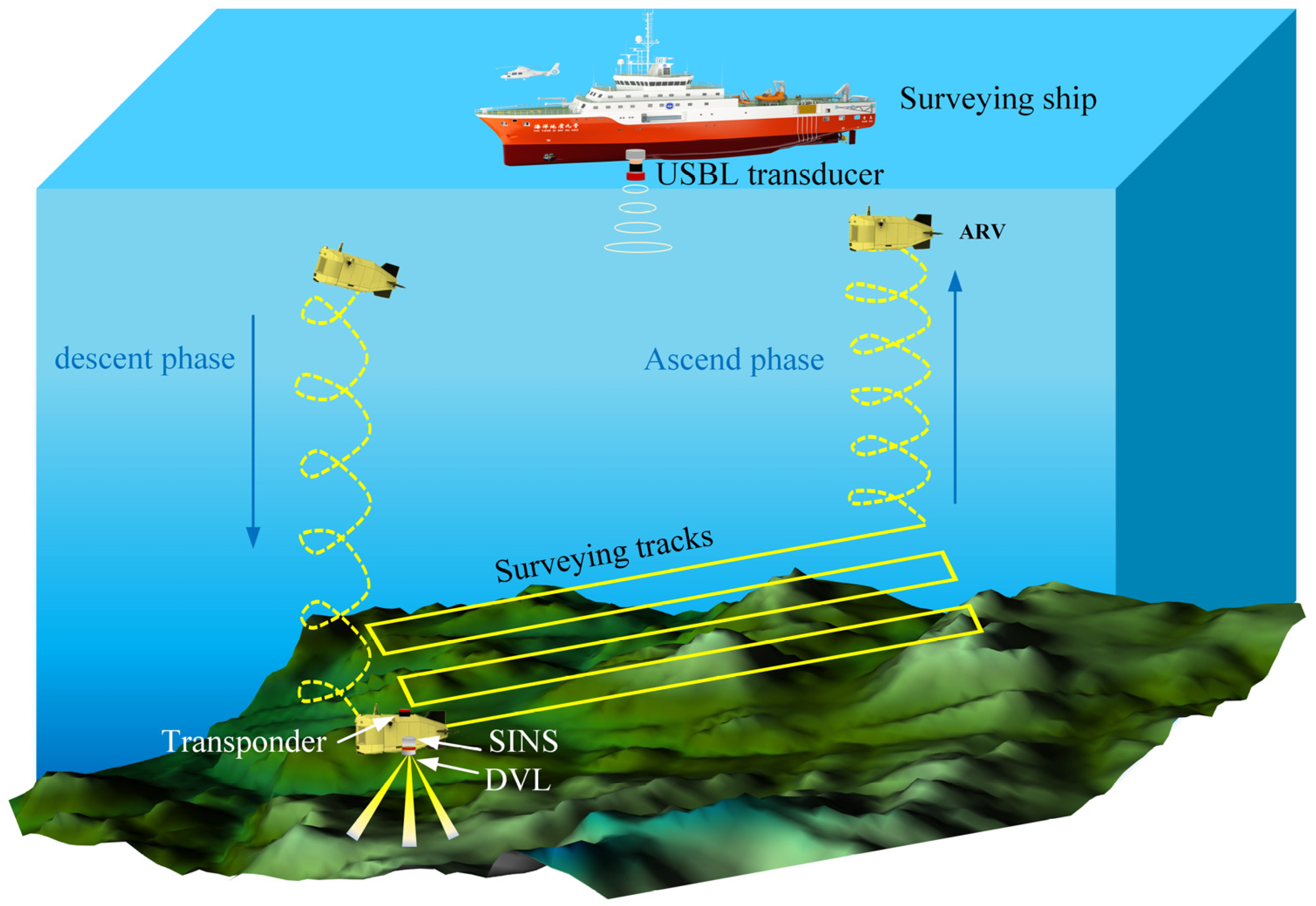
The submersible ARV system combines autonomous navigation and remote control capabilities. In the cable-controlled remote mode, ARV utilizes optical fiber micro-cables for real-time remote control to explore detailed seafloor terrain, shallow subsurface structures, and seafloor surface targets and to take samples of specific targets [35,36]. Furthermore, it can perform autonomous exploration tasks in a hybrid mode of autonomous and remote control. Through real-time transmission of on-site operation information via optical fiber micro-cables, the operator can switch between autonomous navigation and real-time remote control at any time, efficiently and flexibly completing operational tasks. Generally, the main procedure of conducting a mission involves three phases: the descent phase, the surveying cruise, and the ascending phase, as shown in Figure 1. During the surveying phases, the positioning performance of the USBL system will directly impact the level of task execution for the ARV.
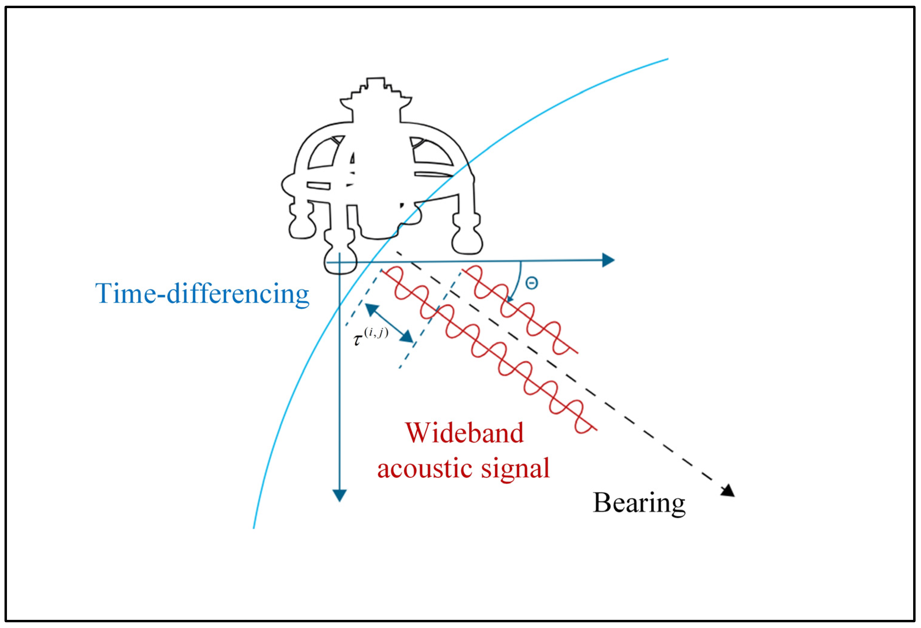
As for the USBL positioning principle, it is typically divided into two categories. For single-frequency narrowband signals, USBL generally locates the target by measuring the phase difference of arrival (PDOA) of different array elements when receiving feedback from the target, while for more widely used broadband signals, USBL adopts time difference of arrival (TDOA) between different array elements to position the underwater target. Without loss of generality, the positioning principle based on TDOA will be depicted as shown in Figure 2. According to the planar approximation of acoustic waves, as in the classical approach presented in reference [37], the direction and the distance between the transponder and the acoustic array are available to compute the relative positions expressed in the ship body frame.
The sub-system of the USBL device typically measures the travel time () between the receiver () of the USBL array and the transponder () mounted on the target by generalized cross-correlation time delay estimation, and is given by
where is the round-trip observed traveling time; for the sake of simplicity, the index is omitted hereinafter. represents the sending time of acoustic signals from the transmitter, denotes the receiving time of feedback acoustic signals for receiver from the transponder, and denotes random and systematic measurement noise involving hardware time delay and common mode noise.
Resorting to the planar wave approximation shown in Figure 1, modified after mature product introduction [38,39], we can present the TDOA between two receivers, and , as
where is the referenced sound speed generally calculated according to the historical sound speed profile, is the position of receiver on the ship body frame, is the TDOA between receivers, and is the normalized directional vector of transponder . stands for the differential noise for the transponder–receiver pair.
Considering all possible combinations of USBL array receivers, the vector of TDOA can be generated by
where , is the traveling time measurement from all receivers given by , and is the difference operator with the size of shown as
Combining Equation (2) with Equation (3) and based on the least square principle, the direction vector for the transponder is given by
where , stands for the relative positions of combinations of receivers, is the position matrix for all receivers with the size of . Note that besides the classical positioning strategy based on TDOA, available direction-of-arrival (DOA) observations along with the TOA make a contribution to centimeter-level repeatability in the locations of geodetic seafloor transponder [37].
According to the planar wave approximation, the range between transponder and the origin of the body frame can be calculated by averaging the range estimates from all receivers. The estimate for receiver is given by
The relative position of a transponder depicted in the ship body frame can be computed by
where is typically obtained by averaging Equation (6) for all receivers, .
On the condition of available attitude measurements provided by the Inertial Navigation System (INS) and the absolute positions of the USBL array in the Earth-Centered, Earth-Fixed (ECEF) frame, the absolute positioning information of the target can be obtained. It is noted that the absolute positioning accuracy of the USBL is influenced by acoustic timing noise, referenced SVP errors, uncertainty about GNSS positioning, attitude measurements, bias of USBL installation, and calibration errors.
2.2. Acoustic Ray Bending Correction for USBL Positioning
The relative geometric distance between a transmitter and a receiver is easily transformed by the traveling time of acoustic signals and typical SSV, as shown in Equation (5). However, the referenced SSV tends to result in systematic errors in acoustic ranging measurements because of the ray-bending effect. Ray-tracing theory, which is based on geometrical acoustics deduced by the Helmholtz equation in the Cartesian system, is commonly applied to track the real bent acoustic path. The general expressions of the horizontal propagation distance () and traveling time () of acoustic signals are as follows:
where denotes the sound speed at depth , is the Snell-satisfying ray parameter, and and stand for the depth of the transmitter and transponder, respectively. Note that these expressions are under the assumption that the complex sound speed profile is a stratified medium with a constant sound speed gradient.
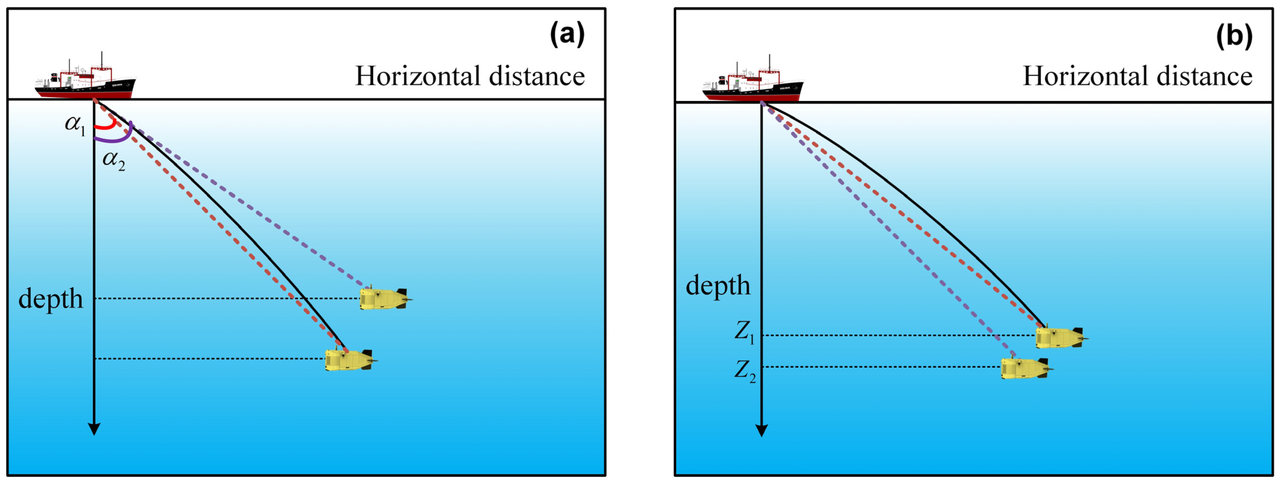
Combined with the acoustic timing measurements and the known real-time positions of the transmitter, the direction angle provided by the USBL system can be used to track acoustic rays on principle, which is defined as one kind of ray tracing direct problem [18]. However, the departure angle of the ray with respect to the vertical plane is referred to as the incident angle, which does not entirely reflect the true direction () of the target as the result of the curved propagation trajectory, as shown in Figure 3. Actually, this angle bias will cause the traced location deviation of the target. In addition to the bearing, as an important data source, depth measurements obtained by the equipped pressure sensor, typically with the superior accuracy of 0.01% range [40], are applied to solve the direct problem, which can be depicted by
where and are the positions of the source and receiver, is the fixed SVP information, and are incident angle and depth observations provided by the USBL and the pressure sensor installed in the ARV, denotes the traveling time of the acoustic signal, and stands for the propagation path length. Observed bearing information can be transformed to obtain the incident angle based on the necessary procedure of coordinate system conversion, which is not within the scope of this contribution but can refer to a series of investigations [41,42]. It is noted that Equation (10) is workable if the incident angle is the initial condition, and Equation (11) is applicable if the depth is the initial condition.
The procedure to solve the aforementioned direct problem is to adopt an incremental accumulation strategy, in which the traveling time of acoustic signals is accumulated layer by layer based on the stratification of SVP. If the incident angle is initial, as depicted in Equation (10), the acoustic path can be inferred towards the receiver and stopped according to the timing observations, which is the maximum threshold. If additional depth information is available, as shown in Equation (11), there is one more step to determine the initial angle by the dichotomy method using the cutoff depth values when compared with the aforementioned case.
Based on the characteristics of the water medium, the initial conditions, and a stopping parameter (traveling time in this scenario), the unique propagation path is tracked and depicted by the direct ray-tracing procedure, and the horizontal distance () of the target is determined simultaneously. Since the relative directional vector between the ship and underwater ARV is available by the USBL system, the traced horizontal distance can be converted to the geometric distance. If the additional depth information is obtainable, the slant distance is converted according to the trigonometric geometric relationship. Thus, the converted geometric distance vector () between the transmitter and the target is available. Equation (5) is rewritten as
Compared with Equation (5), the ranging bias due to the referenced SVV could be weakened by the acoustic ray bending corrected distance observations. Combined with Equations (6) and (12), the positions of ARV can be determined by USBL observations.
2.3. Temporal Sound Speed Correction for USBL Positioning
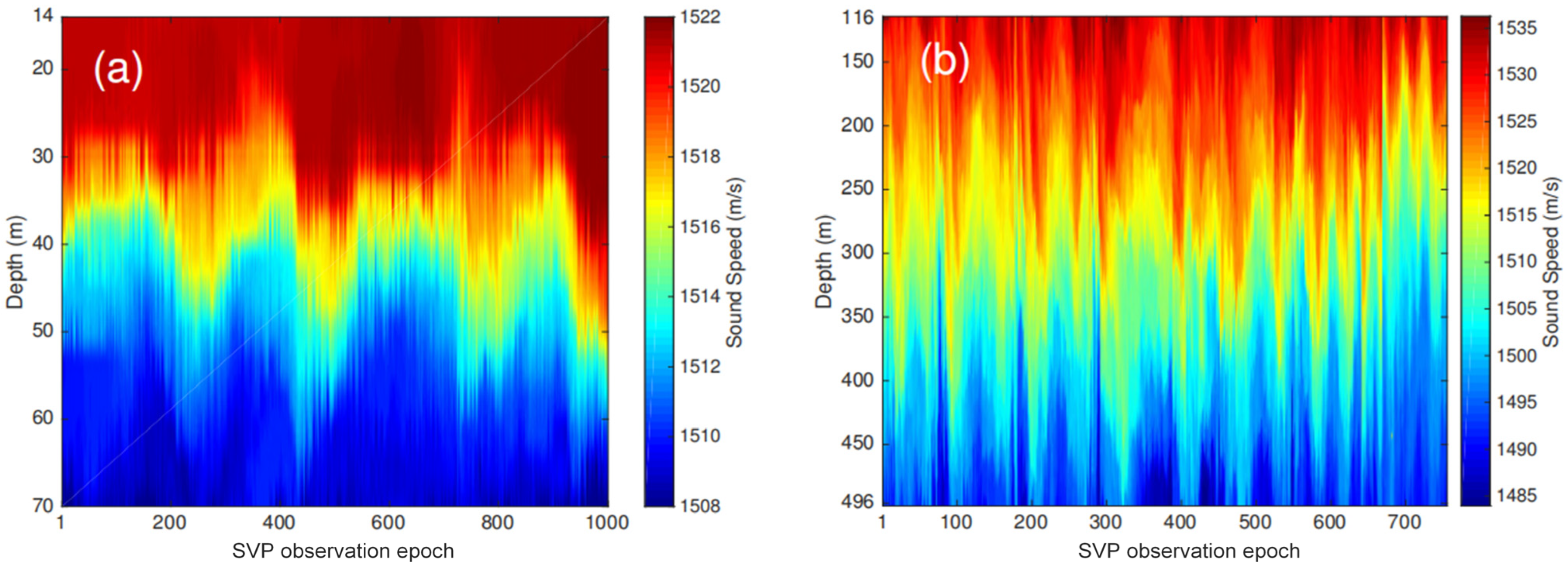
A ray-tracing strategy based on the fixed SVP shows superiority in positioning performance when compared with the referenced SVV commonly adopted in ocean engineering. However, in shallow water, ARVs tend to conduct missions for dozens of hours; meanwhile, the SVP presents temporal variation features due to the changing temperature and depth, as shown in Figure 4, modified after reference [43]. The left subfigure is generated based on the SVP data recorded every 15 s, over a 48 h period, from 14 m to 70 m depth, with 4 m spacing, while the right subfigure is plotted according to CTD data collected at about 1 m resolution from 116 m to 496 m. The fixed SVP could not contain the temporal variation information of SSS; thus, the aforementioned ray-tracing method lacks the potential to correct the time-varying effect of SVP and limit the real-time positioning ability of USBL toward the targets in shallow water.
Given the time-consuming and observation frequency of the sound velocity profiler, it is not easy to collect the real-time vertical-sectional profiles. The only possible access to on-site sound speed information relies on the equipped CTD sensor in the ARV. In this paper, these real-time SVVs are used for temporal sound speed correction in the ARV surveying scenario for shallow water environments. Due to the limited surveying spatial scale of ARVs and the unavailability of the impossible horizontal gradient of sound speed information, temporal correction is conducted under the assumption of homogeneity of SSS.
In-situ sound speed measurements obtained by the equipped sensor of ARV provide the possibility and support to adjust the fixed SVPs, which ignores the time-dependent characteristics. In general, the sound speed varies with each layer: the near-surface layer is more variable than the abyssal one, for example, so the correction function should be estimated for each layer. However, the geometric path of an acoustic wave is almost a straight line because of the smallness of the refractive index [44]. For this reason, the positioning result depends mainly on the average sound speed of all layers. In this analysis, the second step correction of sound speed is not set for each layer but is set uniformly for all the layers. The correction is calculated by the weighted average of the difference of SVV from referenced SVP and SVV from in-situ observations at the same depth index. To weaken the random error effect of on-site measurements, a moving window is applied to ensure the smooth changes of SVV according to the authentic physical characteristics of sound speed variation.
where is the fixed reference SVP, is the in-situ SVV series, is the width of the moving window, is the weight factor, , denotes the degree of time correlation between the observation epoch and selected sampling time in the moving window, and guarantees the robust capability. Once the correction values have been updated, the SVP will be adjusted accordingly, and the corresponding ray-tracing process will be executed again. The unique propagation path is tracked and depicted by the direct ray-tracing procedure, and the horizontal distance () of the target is determined simultaneously. Note that the ray-tracing process is based on resilient SVPs rather than single fixed SVPs. Similarly, the slant distance is converted from the horizontal distance. Thus, the converted geometric distance vector () between the transmitter and the target is available. Equation (5) is rewritten as
Compared with Equation (12), the ranging bias due to the timing-variant SVP could be further attenuated by the correction of sound speed temporal variation. Combined with Equations (6) and (14), the positions of ARV can be determined by USBL observations.
3. Results
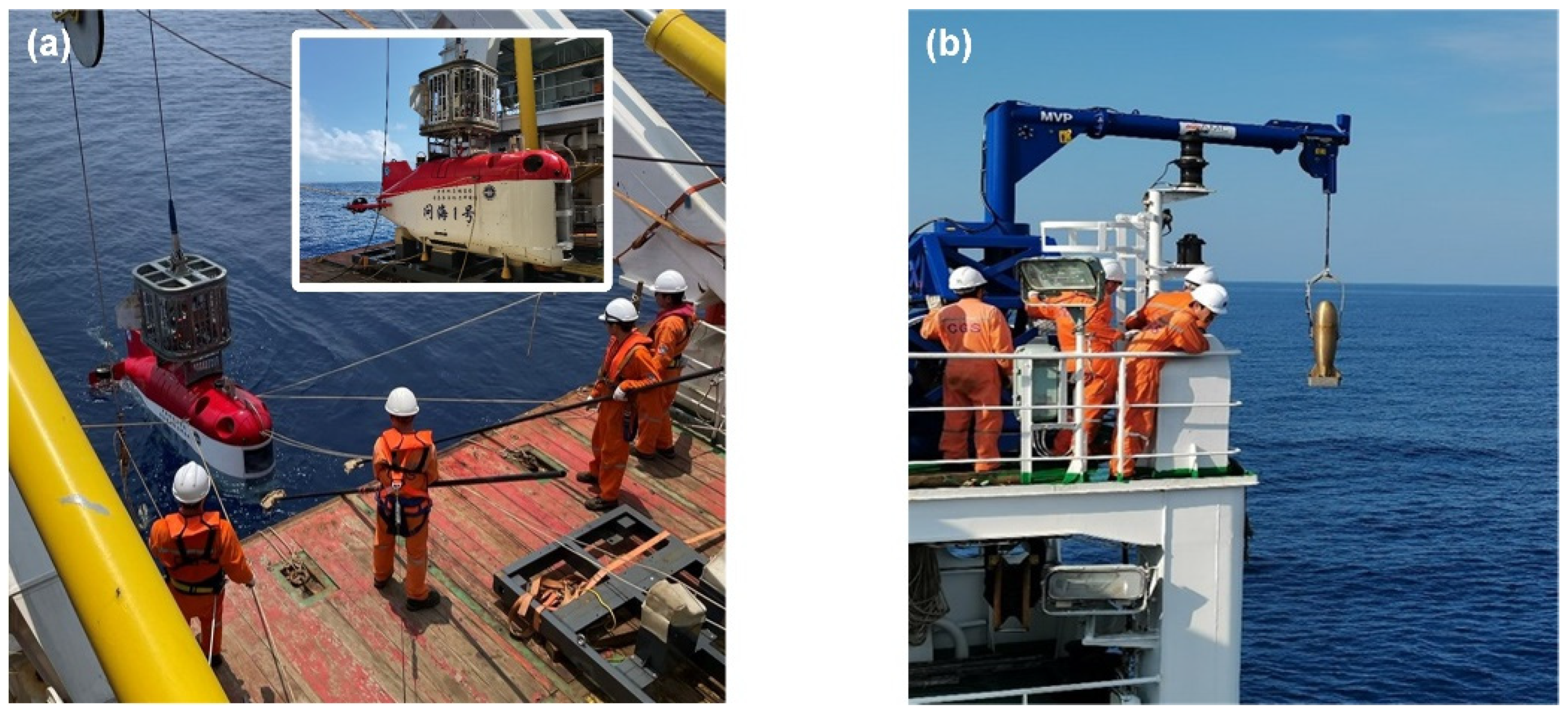
To evaluate the positioning performance of the proposed two-step sound speed correction method, a sea dataset was collected in the South China Sea on 12 April 2022 at a depth of approximately 300 m. The survey was conducted aboard the HYDZ-9 (Hai Yang Di Zhi-9), a ship with dimensions of 87.07 m in length and 17 m in width. During the survey, the sea-surface support ship sailed within the target area while towing the Wenhai-1 ARV, as depicted in Figure 5a, at a specific altitude above the seafloor to carry out surveying tasks. The dataset includes various observations: GNSS measurements provided by Veripos APEX, ship attitudes provided by POS MV 320 of Applanix company (Richmond Hill, ON, Canada), ARV real-time positions provided by the HiPap 102PMGC from the Kongsberg company, real-time sound speed information provided by the CTD sensor installed in the ARV, depth observations provided by the Valeport miniIPS pressure gauge, the height of the ARV above the seafloor obtained by Valeport VA500 altimeter, and sound speed profiles obtained by MVP 300 developed by AML Oceanographic company, as shown in Figure 5b.
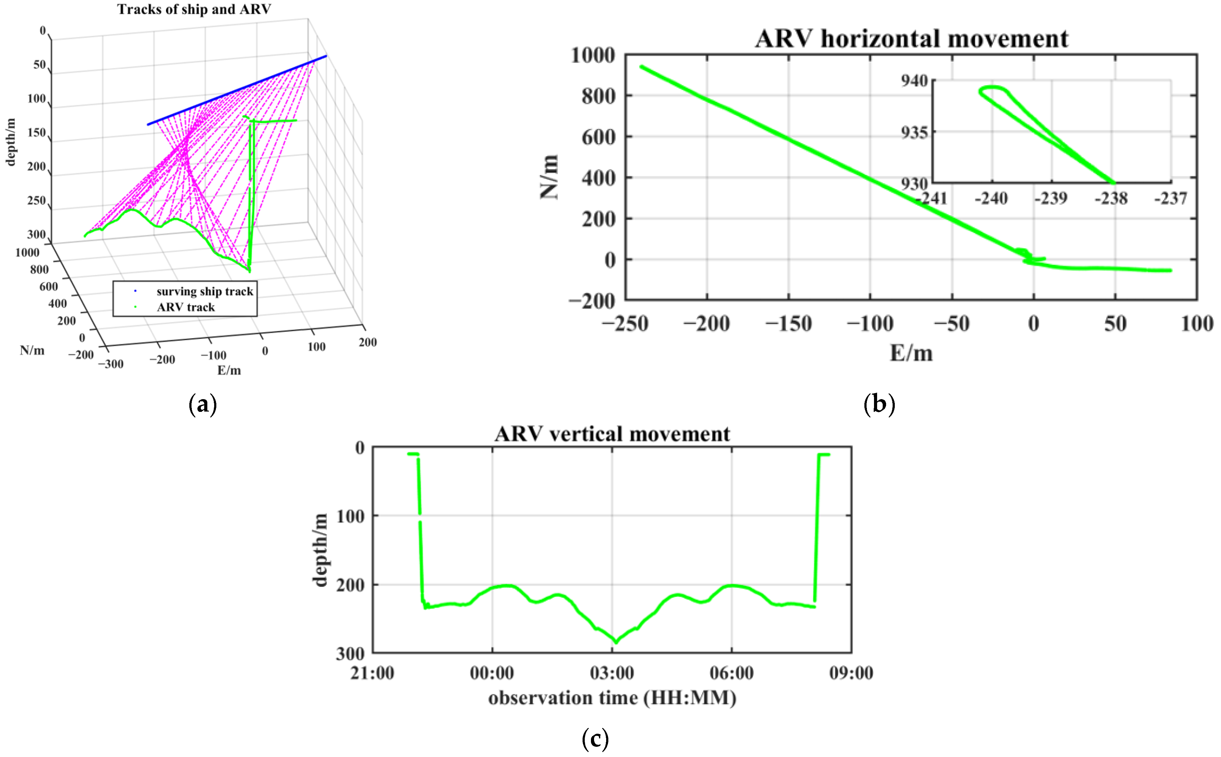
The support ship followed the designated routes on the sea surface while the towed ARV conducted a round-trip cruise towards the seafloor at a fixed height mode. Figure 6a illustrates the complete 3D trajectory of both the ARV and support ship, while Figure 6b displays their horizontal movement tracks. Additionally, Figure 6c depicts the time series of the ARV’s vertical movement, which includes the descent phase, surveying cruise, and ascend phase. Throughout the cruise, the ARV maintained a distance of approximately 50 m from the seabed, and its trajectory showed fluctuation characteristics attributed to the undulating seabed.
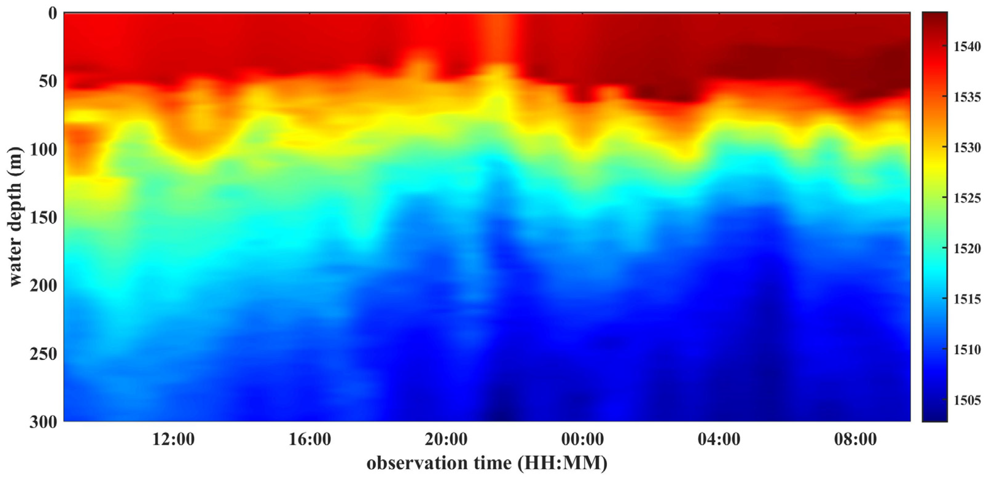
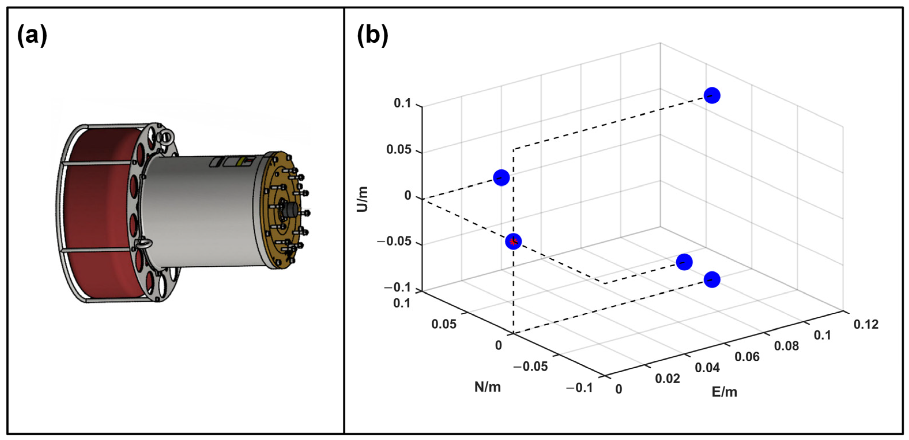
During the sea trial, relatively high-density SVPs are collected approximately every 40 min using the MVP between 07:00 A.M. and 10:00 A.M. on the following day (day + 1). The rendered sound speed profile series, based on the data obtained from 37 profiles, is illustrated in Figure 7. It is evident that the sound speed near the sea surface is significantly faster than that near the seabed, primarily due to temperature variations in the seawater. To obtain acoustic timing observations between the transmitter and the receivers, a semi-physical simulation is employed, as raw timing observations collected by the USBL system are not available. The entire 5-receiver array is compactly assembled within a space of 0.25 square meters, and the designed location layout is shown in Figure 8 as an example.
The conventional approach of using empirical sound speed values is widely employed in the field of ocean engineering applications due to its simplicity and convenience. However, this constant speed value leads to deviations in both the actual slant range and the trajectory due to refraction effects. To address these challenges, the acoustic ray-tracing strategy shows promise by offering different processing procedures based on variant initial conditions, such as incident angles or water depth. To evaluate the performance of direct ray tracing based on both initial conditions, extensive tests were conducted, and the accuracy was assessed in terms of tracing distances. Figure 9 and Figure 10 illustrate the traced results, where the blue and magenta dot lines represent the horizontal and vertical distances, respectively. The error bars depict the standard deviation (STD) based on 100 iterations of tests.
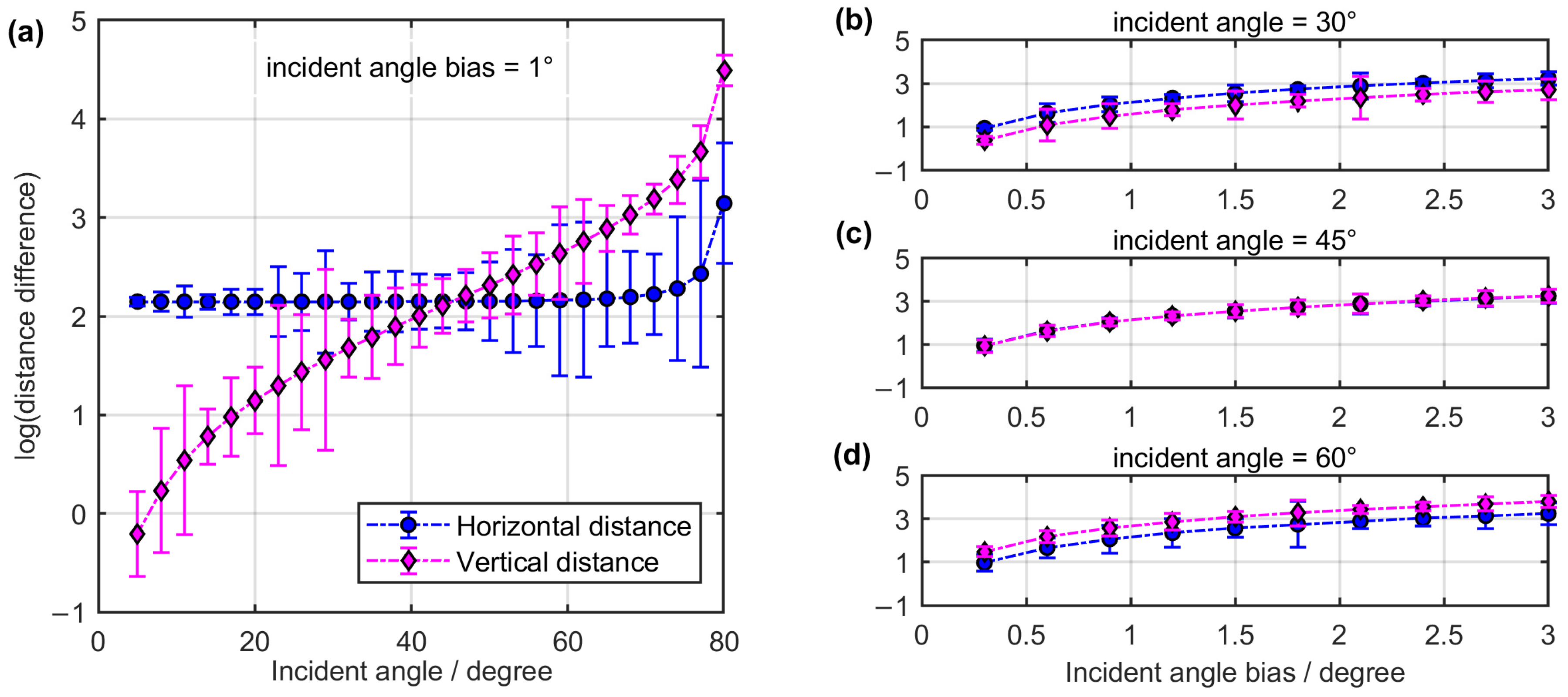
To begin with, the direct tracing performance is evaluated based on the initial angle conditions. There are inevitable deviations between the departure angle of the ray with respect to the vertical plane and the geometric line-of-sight directional angle of the target. For instance, when considering an incident angle bias of 1° at a water depth of 500 m, the traced distances between the acoustic source and the target are obtained. In Figure 9, the longitudinal axis is presented on a logarithmic scale, and the error bars are plotted at 10 times the standard deviation (STD). Figure 9a illustrates the difference between the tracked paths and the geometric paths concerning the incident angle series. As the assumed fixed angle bias increases, the horizontal difference rises significantly with the angles, while the vertical difference remains less sensitive to the variation in angle bias. Notably, at a 60° incident angle, the deviation of horizontal distance exceeds 15 m. Figure 9b–d shows the distance difference due to various angle biases based on incident angles of 30°, 45°, and 60°, respectively. Holistically, an increase in angle bias results in greater deviations in the traced distance. For an incident angle of 45°, variable angle biases have a similar influence on both horizontal and vertical distances. For an incident angle of 30°, angle biases have a greater impact on the horizontal distance compared to the vertical distance. Conversely, for an incident angle of 60°, the opposite trend is observed.
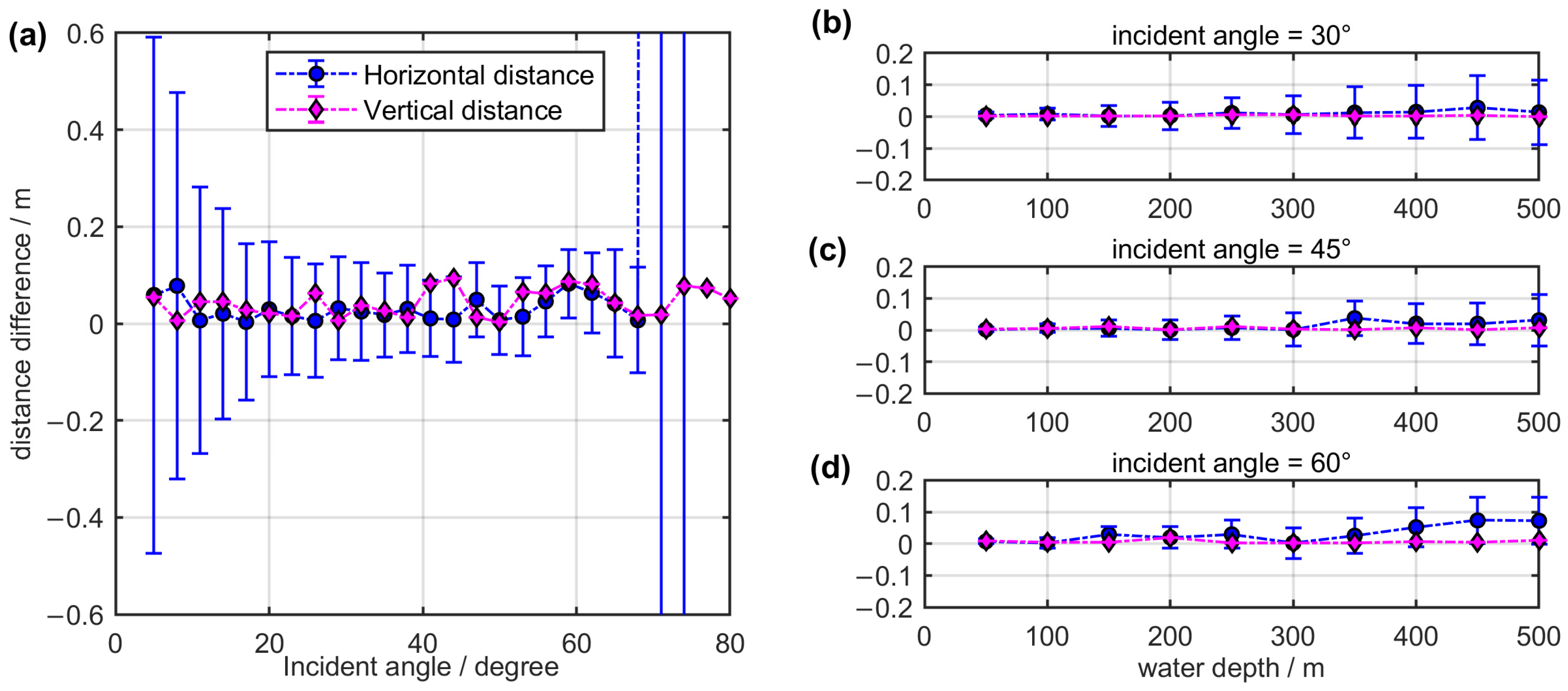
Next, the direct tracing performance is evaluated based on the initial depth conditions. The typical observation accuracy of the pressure sensor is 0.01% of the water depth. For instance, with a water depth of 500 m, we obtain the traced distances between the acoustic source and the target. The horizontal distance deviations are susceptible to both small and large incident angles, while the vertical distance difference mainly depends on the accuracy of the depth sensor, as shown in Figure 10a. Figure 10b–d illustrates the distance differences for various water depths at incident angles of 30°, 45°, and 60°, respectively. Within a series of water depths, the difference between the traced distance and the authentic distance remains evident within ±15 cm in both horizontal and vertical directions, demonstrating higher reliability for target locations. Therefore, we highly recommend adopting the depth-based direct ray-tracing strategy. In the following sections, this approach will be utilized for acoustic ray bending corrections.
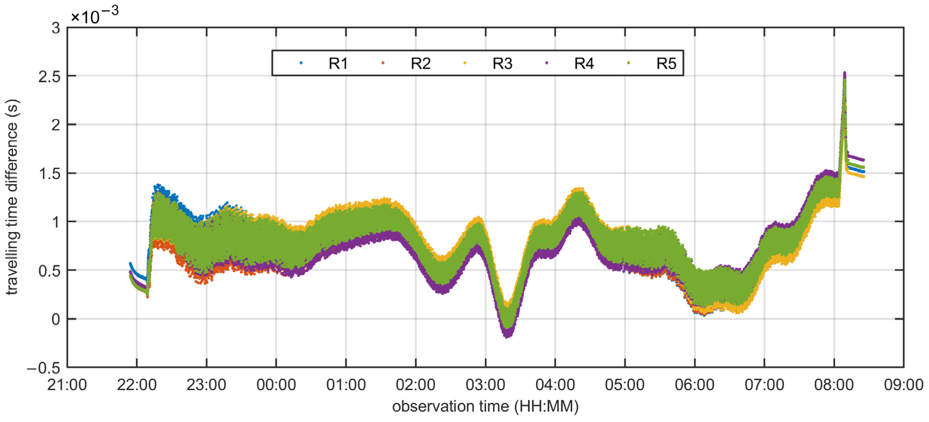
The aforementioned correction method relies on a fixed SVP. However, the time taken for acoustic signals to travel from a specific source to a static target varies due to the temporal fluctuations in the SSS. By incorporating time-varying SVPs, as depicted in Figure 7, and considering the receiver’s installation geometry, as shown in Figure 8b, we obtain more reliable travel time observations based on matched SVPs. Figure 11 illustrates the differences between timing observations based on time-variant SVPs and those based on fixed SVPs, revealing variances on the order of a few milliseconds. This discrepancy is generally larger than the USBL timing accuracy and can lead to systematic ranging errors, thus compromising the USBL positioning performance if the temporal variation of SSS is not considered. Given the limited array space and the assembly of five receivers, the time differences corresponding to these receivers exhibit similar changing trends.
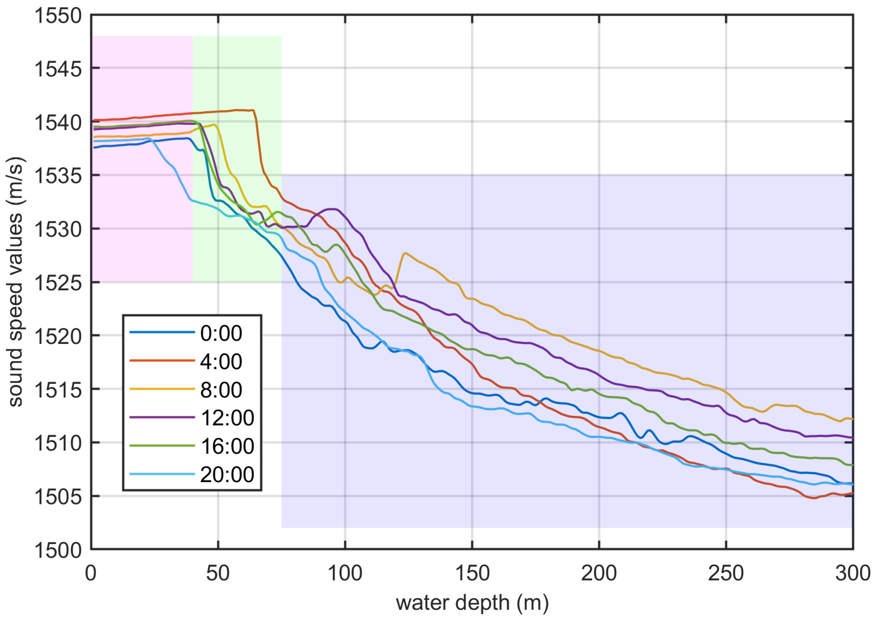
To analyze the authentic temporal variation features of SSS, we have plotted hourly selected SVPs from a data series collected by the MVP within a truncated water depth of 300 m, as depicted in Figure 12. The plot aims to present the general trends without sacrificing generality. Within the top 40 m scale, the sound speed changes slowly, indicated by the pink block. However, beyond a water depth of 40 m, the sound speed slows down rapidly, represented by the green zones. Notably, within the purple zones, which constitute the majority of the profiles, the temporal variation of sound speed exhibits regular and stable patterns. These areas account for the primary changes in the traced traveling time based on the variant SVPs.
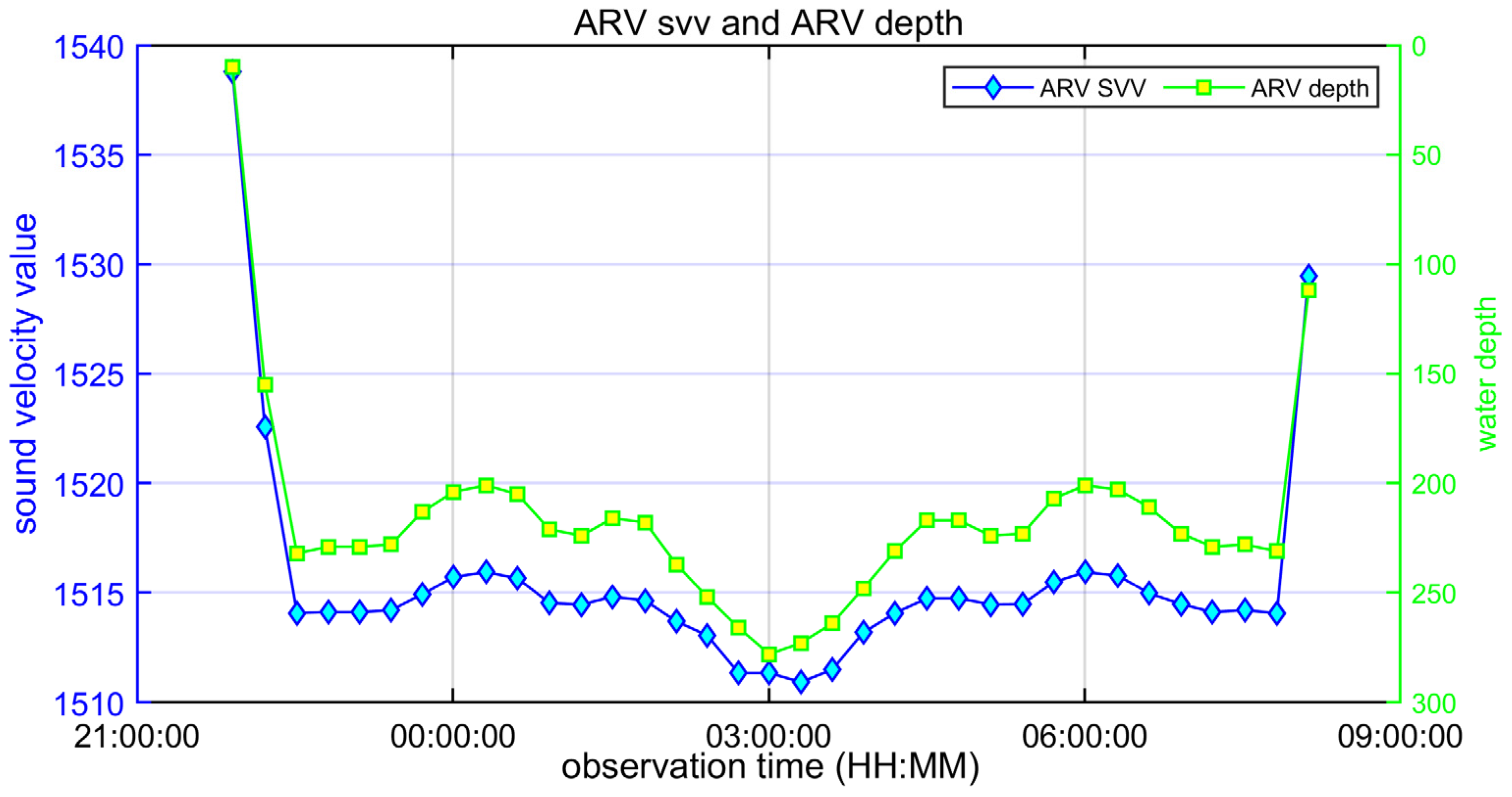
CTD sensors installed on the ARV can provide real-time, on-site sound speed information, which is crucial for further correcting temporal variations relative to fixed SVPs. Figure 13 illustrates selected sound speed values and the corresponding ARV depth at approximately 40 min intervals during the sailing period. The in-situ sound speed undulation shows a consistent pattern with the fluctuations in submarine topography, particularly during the surveying phase. The in-situ SVV measurements reveal a strong correlation between sound speed and depth when the ARV conducts a 50 m undulating survey over the seabed at a depth of 300 m. Each acoustic-ranging epoch is associated with a specific SVP that matches the real path traveled by the acoustic signals. The measurements provided by the CTD sensor serve as anchor points, depicting the relatively stable variation in the time series of SVPs in shallow water.
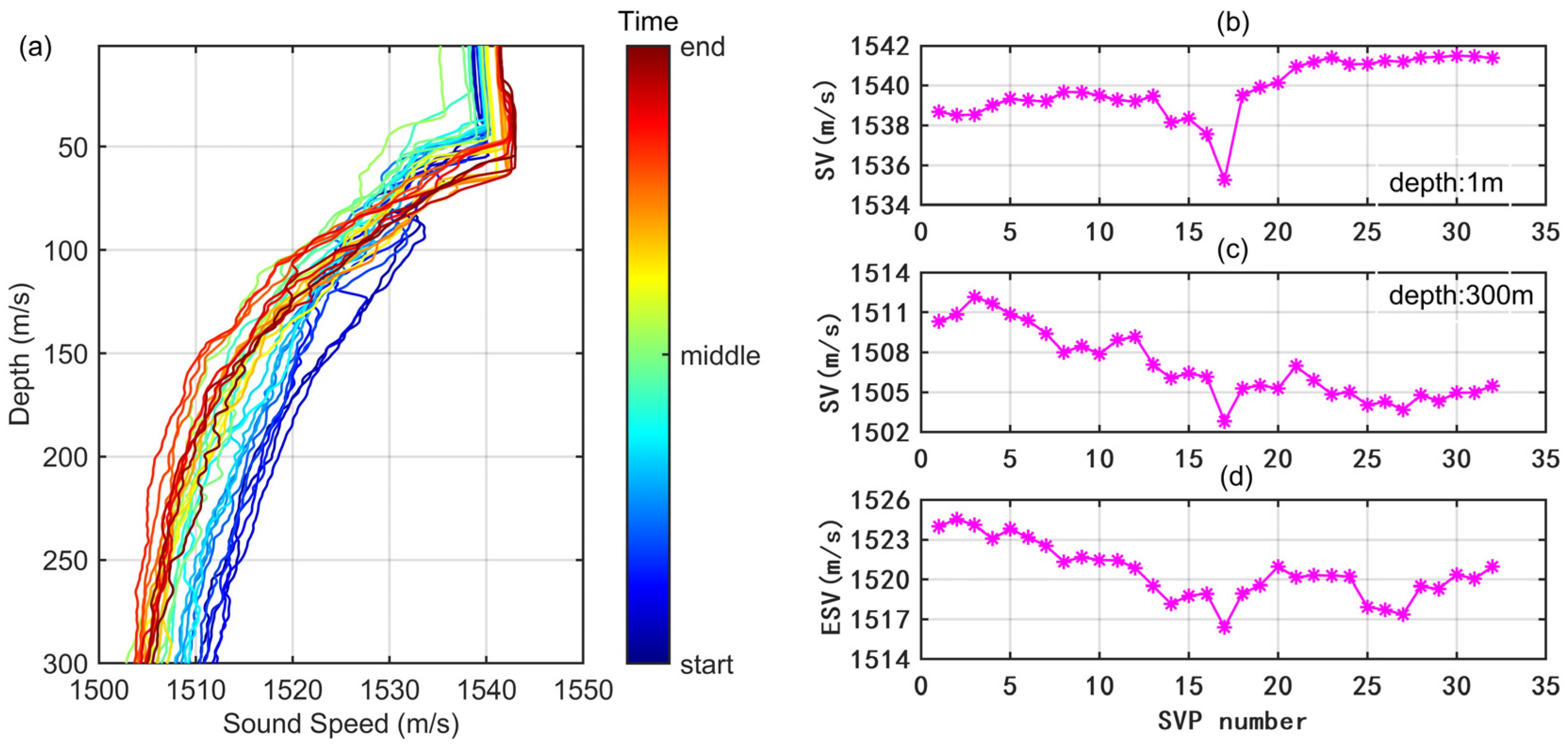
To verify the effectiveness of correction of sound speed temporal variation by using the in-situ sound speed information, the equivalent sound speeds for a total of 37 profiles are calculated and compared with the corresponding SVs at the typical depths, as shown in Figure 14. From the bottom to the top of the color bar, it indicates the chronological order of observations. It shows relatively stable and roughly translational features of temporal variation of sound speed structure at water depth greater than 100 m, which is a foundation to use the in-situ SVs to correct the fixed SVP. Figure 14b,c presents the SVs corresponding to the epoch of the SVP series at the depth of 1 m and 300 m, respectively. The efficient SVs of each fixed SVP corresponding to the full depth are calculated and depicted in Figure 14d. It indicates that the SV at the water layer near the seafloor is more representative of temporal variation trends. Without losing generality, tested depth series’ are further selected. The corresponding SVPs are generated, and ESVs are calculated accordingly. Then, we calculated the correlation coefficient between the in-situ SVs and the ESVs of the fixed SVPs. Table 1 lists the statistical results. The in-situ SVs measurements provided by ARV, which is generally cruising within a water depth range of 250 to 300 m for this offshore experiment, according to Figure 6, are strongly related to the ESVs. It is reasonable to utilize the in-situ measurements to correct the temporal variation of sound speed structure.
Three calculation methods are performed.
- M1—the ARV’s position was calculated by using the constant sound speed value method.
- M2—the ARV’s position was calculated by using the typical correction method based on fixed SVP.
- M3—the ARV’s position was calculated by using the proposed two-step sound speed correction method.
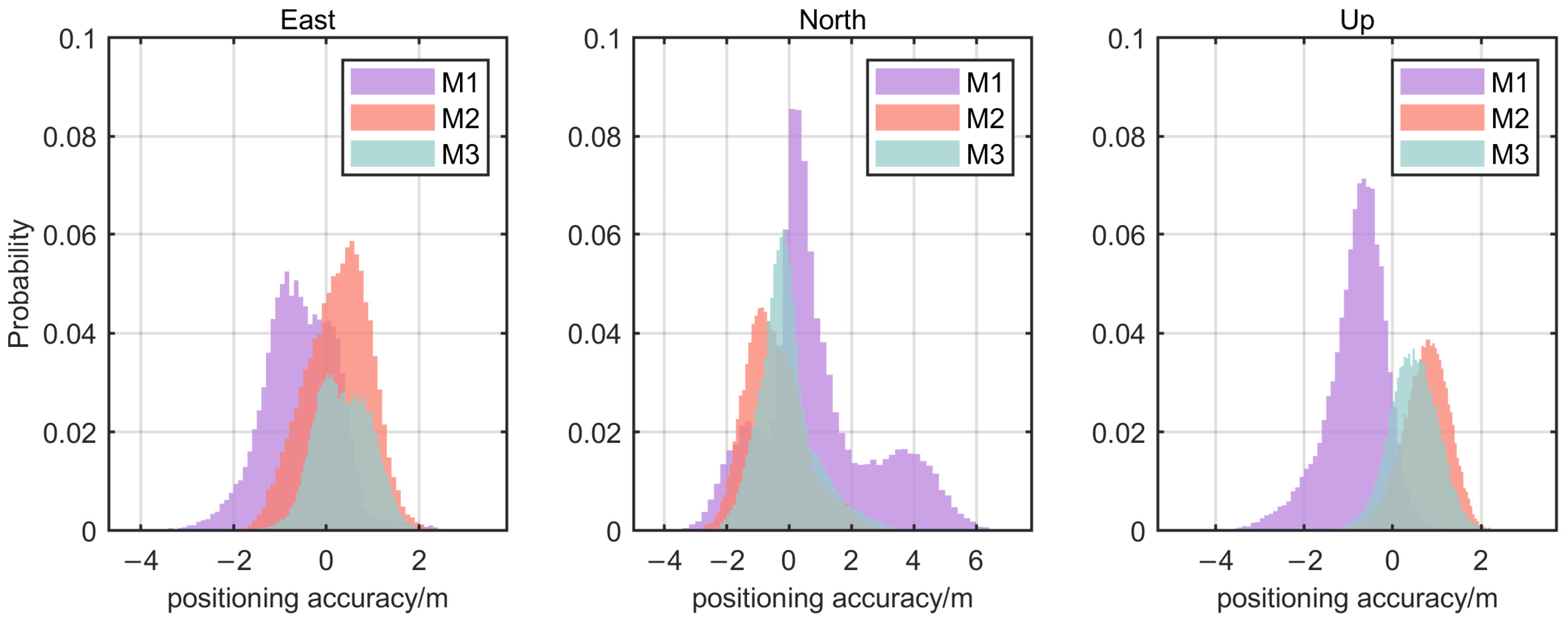
Positioning errors in the east, north, and up directions are shown in Figure 15. The constant sound speed approach introduces systematic ranging errors due to the disparity between the geometric distance and the curved acoustic path. The positioning errors with the M1 method are represented by the purple histogram and display a multimodal distribution, especially in the north direction. The multimodal phenomenon is partially alleviated by applying the ray-tracing method, which accounts for acoustic ray bending errors, resulting in improved positioning performance. Furthermore, the proposed two-step sound speed correction method shows even better results. Intuitively, the frequency histogram’s mode with the M3 method is smaller than that observed with either the M1 or M2 methods, indicating more accurate and consistent positioning outcomes.
Table 2 presents the detailed statistics of positioning errors using three different methods. The M1 method exhibits an evident positioning deviation of more than 1 m in the north direction. On the other hand, the fixed SVP method shows an average improvement of 22% in positioning accuracy in the east direction, 40% in the north direction, and 7% in the up direction compared to the initial fixed SVV method. The ray-tracing policy demonstrates superior horizontal positioning improvement, especially in the north component, which is significantly influenced by the depth-based direct ray-tracing strategy. The positioning accuracy in the vertical component slightly improves due to the observation capability of the depth sensor, effectively reducing the main effect resulting from acoustic ray bending. The residual error source at the ranging level is attributed to the temporal variation of sound speed information, even after accounting for the acoustic ray bending effect. To address this limitation, we propose a two-step method that adjusts the fixed SVP based on in-situ sound speed measurements. With this approach, the positioning accuracy in the east, north, and up directions significantly improves by 28%, 53%, and 31%, respectively, compared to the fixed-SVV method, and by 8%, 21%, and 26%, respectively, compared to the fixed-SVP method. Judging from the standard deviation (STD) values, the proposed two-step correction method demonstrates a more stable positioning performance than the traditional fixed-SVV and fixed-SVP methods; this provides significant advantages in accurate sampling, submarine docking, and precise obstacle avoidance during underwater operations.
4. Conclusions
To enhance the real-time positioning accuracy of the USBL system for towed ARVs, this article proposes a two-step sound speed correction method by dynamically adjusting the SVP based on the in-situ sound speed measurements. The aim is to mitigate the impact of fixed sound speed on acoustic ranging errors. After validating the method through semi-physical simulations and sea-trial datasets, the following conclusions have been drawn:
- The difference in horizontal distance between the geometric path and the curvature route is more susceptible to the incident angle bias than to the depth bias when using the direct ray-tracing method for acoustic ray bending correction. Therefore, it is highly recommended to employ the depth-based direct ray-tracing strategy;
- SVPs corresponding to the main layers of the depth profile exhibit relatively stable temporal variations. The in-situ sound velocity measurements, which contain the temporal variation information, allow for dynamic adjustments to the fixed SVP;
- When compared with the fixed-SVV method, the fixed-SVP method, which adopts the depth-based ray-tracing policy and significantly corrects horizontal deviation caused by the acoustic ray bending effect, leads to improved averaged positioning accuracy in the east, north, and up directions by 22%, 40%, and 7%, respectively;
- Additionally, the two-step resilient-SVP method, which further corrects SVP timing-variant errors, demonstrates improved averaged positioning accuracy in the east, north, and up directions by 8%, 21%, and 26%, respectively, when compared to the fixed-SVP method; this indicates that the two-step resilient-SVP method enhances the adaptability of sound speed observations and shows better performance in real-time USBL positioning.
Author Contributions
Conceptualization, S.Z. and H.L.; methodology, S.Z., H.L. and S.X.; software, S.Z., H.L. and Z.X.; formal analysis and investigation, S.Z., H.L., S.X. and Z.W.; writing—original draft preparation, S.Z.; writing—review and editing, S.X., Z.W. and H.L.; project administration and funding acquisition, S.Z., S.X. and Z.W. All authors have read and agreed to the published version of the manuscript.
Funding
This research was funded by the National Natural Science Foundation of China (grant numbers 41931076, 42174020, and 42304040), the Laoshan Laboratory (grant number LSKJ202205105), the National Key Research and Development Program of China (grant number 2020YFB0505802), the State Key Laboratory of Geo-Information Engineering (grant number SKLGIE2020-M-1-1), the National Natural Science Foundation of China (grant number 42174021), and the Fundamental Research Fund for Central Universities (grant number 22CX06032A).
Data Availability Statement
All data included in this study are available upon reasonable request from the corresponding author.
Acknowledgments
The authors would like to thank many members of staff of the Qingdao Institute of Marine Geology, China Geological Survey, including the crew of the survey vessel HYDZ-9, who supported our observations and technological developments. The authors also thank the editor and reviewers for their comments and suggestions, which greatly improved the content of this article.
Conflicts of Interest
The authors declare no conflict of interest.
References
- Urick, R.J. Principles of Underwater Sound, 3rd ed.; Peninsula Pub: Baileys Harbor, WI, USA, 1996. [Google Scholar]
- Kussat, N.H.; Chadwell, C.D.; Zimmerman, R. Absolute positioning of an autonomous underwater vehicle using GPS and acoustic measurements. IEEE J. Ocean. Eng. 2005, 30, 153–164. [Google Scholar] [CrossRef]
- Maki, T.; Matsuda, T.; Sakamaki, T.; Ura, T.; Kojima, J. Navigation method for underwater vehicles based on mutual acoustical positioning with a single seafloor station. IEEE J. Ocean. Eng. 2013, 38, 167–177. [Google Scholar] [CrossRef]
- Chen, H.; Wang, C. Accuracy assessment of GPS/Acoustic positioning using a Seafloor Acoustic Transponder System. Ocean Eng. 2011, 38, 1472–1479. [Google Scholar] [CrossRef]
- Reis, J.; Morgado, M.; Batista, P.; Oliveira, P.; Silvestre, C. Design and experimental validation of a USBL underwater acoustic positioning system. Sensors 2016, 16, 1491. [Google Scholar] [CrossRef]
- Graça, P.A.A. Relative Acoustic Localization with USBL (Ultra-Short Baseline). Master’s Thesis, University of Porto, Porto, Portugal, 2020. [Google Scholar]
- Zhang, J.; Han, Y.; Zheng, C.; Sun, D. Underwater target localization using long baseline positioning system. Appl. Acoust. 2016, 111, 129–134. [Google Scholar] [CrossRef]
- Luo, Q.; Yan, X.; Wang, C.; Shao, Y.; Zhou, Z.; Li, J.; Hu, C.; Wang, C.; Ding, J. A SINS/DVL/USBL integrated navigation and positioning IoT system with multiple sources fusion and federated Kalman filter. J. Cloud Comput. 2022, 11, 18. [Google Scholar] [CrossRef]
- Liu, H.; Wang, Z.; Shan, R.; He, K.; Zhao, S. Research into the integrated navigation of a deep-sea towed vehicle with USBL/DVL and pressure gauge. Appl. Acoust. 2020, 159, 107052. [Google Scholar] [CrossRef]
- Vickery, K. Acoustic positioning systems: A practical overview of current systems. In Proceedings of the 1998 Workshop on Autonomous Underwater Vehicles, Cambidge, MA, USA, 21 August 1998; IEEE: Piscataway, NJ, USA, 1998. [Google Scholar]
- Tong, J.; Xu, X.; Zhang, T.; Li, Y.; Yao, Y.; Weng, C.; Hou, L.; Zhang, L. A misalignment angle error calibration method of underwater acoustic array in strapdown inertial navigation system/ultrashort baseline integrated navigation system based on single transponder mode. Rev. Sci. Instrum. 2019, 90, 085001. [Google Scholar] [CrossRef]
- Chen, H.-H. The estimation of angular misalignments for ultra short baseline navigation systems. Part II: Experimental results. J. Navig. 2013, 66, 773–787. [Google Scholar] [CrossRef]
- Zhu, Y.; Zhang, T.; Xu, S.; Shin, H.-S.; Li, P.; Jin, B.; Zhang, L.; Weng, C.; Li, Y. A calibration method of USBL installation error based on attitude determination. IEEE Trans. Veh. Technol. 2020, 69, 8317–8328. [Google Scholar] [CrossRef]
- Zhao, S.; Wang, Z.; Nie, Z.; He, K.; Ding, N. Investigation on total adjustment of the transducer and seafloor transponder for GNSS/Acoustic precise underwater point positioning. Ocean Eng. 2021, 221, 108533. [Google Scholar] [CrossRef]
- Van de Voort, N. Inversion Methods of the Sound Velocity Profile for Improving the Accuracy of the USBL Positioning System. Ph.D. Thesis, Delft University of Technology, Delft, The Netherlands, 2022. [Google Scholar]
- Zhao, S.; Wang, Z.; He, K.; Ding, N. Investigation on underwater positioning stochastic model based on acoustic ray incidence angle. Appl. Ocean Res. 2018, 77, 69–77. [Google Scholar] [CrossRef]
- Sun, D.; Li, H.; Zheng, C.; Li, X. Sound velocity correction based on effective sound velocity for underwater acoustic positioning systems. Appl. Acoust. 2019, 151, 55–62. [Google Scholar] [CrossRef]
- Sakic, P.; Ballu, V.; Crawford, W.; Wöppelmann, G. Acoustic ray tracing comparisons in the context of geodetic precise off-shore positioning experiments. Mar. Geod. 2018, 41, 315–330. [Google Scholar] [CrossRef]
- Chadwell, C.; Sweeney, A. Acoustic Ray-Trace Equations for Seafloor Geodesy. Mar. Geod. 2010, 33, 164–186. [Google Scholar] [CrossRef]
- He, C.; Wang, Y.; Yu, W.; Song, L. Underwater target localization and synchronization for a distributed SIMO Sonar with an isogradient SSP and uncertainties in receiver locations. Sensors 2019, 19, 1976. [Google Scholar] [CrossRef]
- Ameer, P.M.; Jacob, L. Localization using ray tracing for underwater acoustic sensor networks. IEEE Commun. Lett. 2010, 14, 930–932. [Google Scholar] [CrossRef]
- Zhao, J.; Liu, J. Multibeam Bathymetry and Image Data Processing; Wuhan University Press: Wuhan, China, 2008. [Google Scholar]
- Rousselet, L.; Doglioli, A.M.; de Verneil, A.; Pietri, A.; Della Penna, A.; Berline, L.; Marrec, P.; Grégori, G.; Thyssen, M.; Carlotti, F.; et al. Vertical motions and their effects on a biogeochemical tracer in a cyclonic structure finely observed in the Ligurian Sea. J. Geophys. Res. Ocean. 2019, 124, 3561–3574. [Google Scholar] [CrossRef]
- Church, I.W. Multibeam sonar ray-tracing uncertainty evaluation from a hydrodynamic model in a highly stratified estuary. Mar. Geod. 2020, 43, 359–375. [Google Scholar] [CrossRef]
- Shao, M.; Ortiz-Suslow, D.G.; Haus, B.K.; Lund, B.; Williams, N.J.; Özgökmen, T.M.; Laxague, N.J.; Horstmann, J.; Klymak, J.M.J.J.O.G.R.O. The variability of winds and fluxes observed near submesoscale fronts. J. Geophys. Res. Ocean. 2019, 124, 7756–7780. [Google Scholar] [CrossRef]
- Watanabe, S.; Ishikawa, T.; Yokota, Y.; Nakamura, Y. GARPOS: Analysis software for the GNSS-A seafloor positioning with simultaneous estimation of sound speed structure. Front. Earth Sci. 2020, 8, 597532. [Google Scholar] [CrossRef]
- Yokota, Y.; Ishikawa, T.; Watanabe, S. Gradient field of undersea sound speed structure extracted from the GNSS-A oceanography. Mar. Geophys. Res. 2019, 40, 493–504. [Google Scholar] [CrossRef]
- Honsho, C.; Kido, M.; Tomita, F.; Uchida, N. Offshore postseismic deformation of the 2011 Tohoku earthquake revisited: Application of an improved GPS-acoustic positioning method considering horizontal gradient of sound speed structure. J. Geophys. Res. Solid Earth 2019, 124, 5990–6009. [Google Scholar] [CrossRef]
- Yang, Y.; Qin, X. Resilient observation models for seafloor geodetic positioning. J. Geod. 2021, 95, 79. [Google Scholar] [CrossRef]
- Xu, P.; Ando, M.; Tadokoro, K. Precise, three-dimensional seafloor geodetic deformation measurements using difference techniques. Earth Planets Space 2005, 57, 795–808. [Google Scholar] [CrossRef]
- Xue, S.; Yang, Y.; Yang, W. Single-differenced models for GNSS-acoustic seafloor point positioning. J. Geod. 2022, 96, 38. [Google Scholar] [CrossRef]
- Wang, Z.; Zhao, S.; Ji, S.; He, K.; Nie, Z.; Liu, H.; Shan, R. Real-time stochastic model for precise underwater positioning. Appl. Acoust. 2019, 150, 36–43. [Google Scholar] [CrossRef]
- Zhao, S.; Wang, Z.; He, K.; Nie, Z.; Liu, H.; Ding, N. Investigation on stochastic model refinement for precise underwater positioning. IEEE J. Ocean. Eng. 2020, 45, 1482–1496. [Google Scholar] [CrossRef]
- Yokota, Y.; Kaneda, M.; Hashimoto, T.; Yamaura, S.; Kouno, K.; Hirakawa, Y. Experimental verification of seafloor crustal deformation observations by UAV-based GNSS-A. Sci. Rep. 2023, 13, 4105. [Google Scholar] [CrossRef]
- Tadokoro, K.; Kinugasa, N.; Kato, T.; Terada, Y.; Matsuhiro, K. A Marine-buoy-mounted system for continuous and real-time measurment of seafloor crustal deformation. Front. Earth Sci. 2020, 8, 123. [Google Scholar] [CrossRef]
- Iinuma, T.; Kido, M.; Ohta, Y.; Fukuda, T.; Tomita, F.; Ueki, I. GNSS-Acoustic observations of seafloor crustal deformation using a wave glider. Front. Earth Sci. 2021, 9, 87. [Google Scholar] [CrossRef]
- Yli-Hietanen, J.; Kalliojarvi, K.; Astola, J. Low-complexity angle of arrival estimation of wideband signals using small arrays. In Proceedings of the 8th Workshop on Statistical Signal and Array Processing, Corfu, Greece, 24–26 June 1996; IEEE: Piscataway, NJ, USA, 1996. [Google Scholar]
- iXblue Corp. Homepage. Available online: https://www.ixblue.com/ (accessed on 17 October 2023).
- Konsberg Corp. Homepage. Available online: https://www.kongsberg.com/ (accessed on 17 October 2023).
- Sakic, P.; Chupin, C.; Ballu, V.; Coulombier, T.; Morvan, P.-Y.; Urvoas, P.; Beauverger, M.; Royer, J.-Y. Geodetic seafloor positioning using an unmanned surface vehicle—Contribution of direction-of-arrival observations. Front. Earth Sci. 2021, 9, 636156. [Google Scholar] [CrossRef]
- Liu, H. Research on the Underwater Vehicle Integrated Navigation Based on Bayesian Filter[D]; Chinese University of Petroleum: Beijing, China, 2020. [Google Scholar]
- Tong, J.; Xu, X.; Zhao, T.; Zhang, T.; Zhang, L.; Li, Y. Study on installation error analysis and calibration of acoustic transceiver array based on SINS/USBL integrated system. IEEE Access 2018, 6, 66923–66939. [Google Scholar]
- Bianco, M.; Gerstoft, P. Dictionary learning of sound speed profiles. J. Acoust. Soc. Am. 2017, 141, 1749–1758. [Google Scholar] [CrossRef]
- Yokota, Y.; Ishikawa, T.; Watanabe, S. Seafloor crustal deformation data along the subduction zones around Japan obtained by GNSS-A observations. Sci. Data 2018, 5, 180182. [Google Scholar] [CrossRef]
Figure 1.
Sketch map of ARV surveying phases in shallow water. Acoustic array of USBL is mounted at the bottom of the surveying ship. The acoustic transponder is equipped at the ARV. The blue arrow represents the direction of movement, and the yellow curve and round-trip zigzag represent the spiral lifting trajectory and cruise track, respectively.

Figure 2.
Sketch map of planar wave approximation for USBL positioning. Red cureves stand for the paths of wideband acoustic signals, and blue line with arrows denotes the time difference of arrival.
Figure 2.
Sketch map of planar wave approximation for USBL positioning. Red cureves stand for the paths of wideband acoustic signals, and blue line with arrows denotes the time difference of arrival.

Figure 3.
Comparison of ray tracing direct problem based on the obtained incident angle information (a) and the depth observations (b). The target determined by the black straight lines stands for the true location with respect to the incident angle () and depth (), while that determined by the purple lines denotes the tracked result with respect to the incident angle () and depth ().

Figure 4.
Temporal variation of SVP at shallow water depth. (a) SVP measurement was conducted off the coast of Point Loma, CA; (b) CTD data were collected across the Luzon Strait near the South China Sea (SCS).
Figure 4.
Temporal variation of SVP at shallow water depth. (a) SVP measurement was conducted off the coast of Point Loma, CA; (b) CTD data were collected across the Luzon Strait near the South China Sea (SCS).

Figure 5.
(a) An ARV named “Wen Hai—1” was employed during the sea trail at the South China Sea, and the name of ARV in Chinese is sprayed on the metal shell; (b) MVP was applied to collect time series SVP data.
Figure 5.
(a) An ARV named “Wen Hai—1” was employed during the sea trail at the South China Sea, and the name of ARV in Chinese is sprayed on the metal shell; (b) MVP was applied to collect time series SVP data.

Figure 6.
Sketch map of the ARV and support ship trajectories. (a) A 3D view of surveying tracks, magenta lines stand for the relative positions between the sea-surface ship and the towed ARV; (b) horizontal movement tracks of ARV; the subfigure in the upper right corner shows the turning session; and (c) vertical movement time series of the ARV at the “fixed height mode.”

Figure 7.
Time series of SVPs collected by the MVP during 07:00 A.M.~10:00 A.M. (day + 1). The left axis denotes water depth, and the right color bar denotes the sound velocity values.
Figure 7.
Time series of SVPs collected by the MVP during 07:00 A.M.~10:00 A.M. (day + 1). The left axis denotes water depth, and the right color bar denotes the sound velocity values.

Figure 8.
(a) External view of the portable USBL; (b) layout sketch map of receivers in the USBL array. Blue dots denote for the elements of the acoustic array, and the red point shows the array’s center.
Figure 8.
(a) External view of the portable USBL; (b) layout sketch map of receivers in the USBL array. Blue dots denote for the elements of the acoustic array, and the red point shows the array’s center.

Figure 9.
The common logarithm of the distance difference between the traced and geometric values is evaluated under the initial condition of the incident angle. Specifically, (a) illustrates the distance difference with respect to variable incident angles, assuming a 1° angle bias. Additionally, (b–d) presents the distance difference based on the variable incident angle biases corresponding to incident angles of 30°, 45°, and 60°, respectively.

Figure 10.
The distance difference between the traced and the geometrical values is evaluated under the initial condition of the depth observations. Specifically, (a) illustrates the distance difference regarding variable incident angles at the water depth of 500 m. Additionally, (b–d) shows the distance difference based on variable depth with respect to incident angles 30°, 45° and 60°, respectively.

Figure 11.
Difference between traced propagation time based on fixed SVP and the time-variant SVPs. R1~R5 denotes five receivers in the USBL acoustic array.
Figure 11.
Difference between traced propagation time based on fixed SVP and the time-variant SVPs. R1~R5 denotes five receivers in the USBL acoustic array.

Figure 12.
Comparison diagram of hourly sampling SVPs.

Figure 13.
Time series of on-site sound velocity values and ARV depth.

Figure 14.
The sketch map of the SVP time series and the selected SVs. Specifically, (a) a series of collected SVPs; the color bar shows the observation time sequence involving the start, the middle, and the end. (b) Observed SVs corresponding to the epoch of the SVP series at a depth of 1 m. (c) Observed SVs corresponding to the epoch of the SVP series at a depth of 300 m. (d) ESV of each SVP corresponding to the full depth.

Figure 15.
Histogram for positioning accuracy based on three methods.


Table 1.
Correlation between the in-situ SV at different depths and ESV for the corresponding water depth scope.
Table 1.
Correlation between the in-situ SV at different depths and ESV for the corresponding water depth scope.
| No. | 1 | 2 | 3 | 4 | 5 | 6 | 7 | 8 | 9 |
|---|---|---|---|---|---|---|---|---|---|
| depth (m) | 5 | 10 | 20 | 50 | 100 | 150 | 200 | 250 | 300 |
| correlation | 0.9998 | 0.9999 | 0.9971 | 0.8665 | 0.4235 | 0.5382 | 0.6864 | 0.8401 | 0.8939 |
Table 2.
Positioning performance for three methods (unit: m).
| Methods | Average | STD | ||||
|---|---|---|---|---|---|---|
| E | N | U | E | N | U | |
| M1 | 0.779 | 1.467 | 0.866 | 0.806 | 1.829 | 0.689 |
| M2 | 0.606 | 0.879 | 0.803 | 0.689 | 0.974 | 0.547 |
| M3 | 0.559 | 0.691 | 0.594 | 0.600 | 0.913 | 0.558 |
Disclaimer/Publisher’s Note: The statements, opinions and data contained in all publications are solely those of the individual author(s) and contributor(s) and not of MDPI and/or the editor(s). MDPI and/or the editor(s) disclaim responsibility for any injury to people or property resulting from any ideas, methods, instructions or products referred to in the content. |
© 2023 by the authors. Licensee MDPI, Basel, Switzerland. This article is an open access article distributed under the terms and conditions of the Creative Commons Attribution (CC BY) license (https://creativecommons.org/licenses/by/4.0/).
Share and Cite
MDPI and ACS Style
Zhao, S.; Liu, H.; Xue, S.; Wang, Z.; Xiao, Z. Two-Step Correction Based on In-Situ Sound Speed Measurements for USBL Precise Real-Time Positioning. Remote Sens. 2023, 15, 5046. https://doi.org/10.3390/rs15205046
AMA Style
Zhao S, Liu H, Xue S, Wang Z, Xiao Z. Two-Step Correction Based on In-Situ Sound Speed Measurements for USBL Precise Real-Time Positioning. Remote Sensing. 2023; 15(20):5046. https://doi.org/10.3390/rs15205046
Chicago/Turabian StyleZhao, Shuang, Huimin Liu, Shuqiang Xue, Zhenjie Wang, and Zhen Xiao. 2023. "Two-Step Correction Based on In-Situ Sound Speed Measurements for USBL Precise Real-Time Positioning" Remote Sensing 15, no. 20: 5046. https://doi.org/10.3390/rs15205046
Note that from the first issue of 2016, this journal uses article numbers instead of page numbers. See further details here.